Network-accelerated Distributed Machine Learning Using MLFabric Raajay Viswanathan, and Aditya Akella 2020

Network-accelerated Distributed Machine Learning Using MLfabric

Abstract: Existing distributed machine learning (DML) systems focus on improving the computational efficiency of distributed learning, whereas communication aspects have received less attention. Many DML systems treat the network as a blackbox. Thus, DML algorithms’ performance is impeded by network bottlenecks, and DML systems end up sacrificing important algorithmic and system-level benefits. We present MLfabric, a communication library that manages all network transfers in a DML system, and holistically determines the communication pattern of a DML algorithm at any point in time. This allows MLfabric to carefully order transfers (i.e., gradient updates) to improve convergence, opportunistically aggregate updates in-network to improve efficiency, and proactively replicate some of them to support new notions of fault tolerance. We empirically find that MLfabric achieves up to $3\times$ speed- up in training large deep learning models in realistic dynamic cluster settings.

1 Introduction

Machine learning (ML) is revolutionizing not only the computing industry, but also fields such as healthcare and education, where ML techniques are driving key applications. Thus, there is a race to build new ML systems [6, 1, 5, 33] that efficiently learn complex models from big datasets.

To support large model sizes and training data most systems execute distributed versions of ML (DML) algorithms across 10s-100s of workers in a cluster. These DML algorithms, e.g., distributed stochastic gradient descent (SGD), and distributed Latent Dirichlet Allocation (LDA) [8, 25], are iterative in nature, and are both computation and communication intensive. In each iteration, a worker computes an update to the large model, which then needs to be disseminated to all other workers. Model updates can be $\geq 100$MB per worker per iteration, yielding large network transfers (§2).

Many DML systems [6, 5, 15, 1] focus on addressing the performance of computing updates at individual workers, e.g., via optimal use of hardware accelerators [19, 27]. In contrast, systematically addressing communication efficiency and network bottlenecks has received limited attention. In most systems, the application (DML algorithm) manages both computation and communication. A simple network view, as offering fixed bandwidth between all cluster workers, is adopted. Application-level techniques are then used to reduce total data transferred to/from a worker to avoid network bottlenecks.

DML systems thus treat the network as a blackbox, and as such, are unable to overcome network issues. Consider Parameter Server (PS) based ML systems [33, 10]. The model is stored at a separate location (server); in every iteration workers pull the latest model and compute an update, which is then shipped to the server and applied to the model. PS systems support flexible consistency schemes, e.g., strict synchronous, stale synchronous, or asynchronous model updates (§2), which help improve DML algorithms’ compute efficiency and convergence [23]. However, they deal with network efficiency using ad hoc application-level approaches, such as, dropping updates deemed not significant, or coarsely quantizing updates [33]. Unfortunately, these approaches affect algorithm convergence [30], and yet may not be effective enough in dealing with serious onset of congestion.

Likewise, MPI-based systems [1, 4] — which support only synchronous SGD — employ MPI_AllReduce operations to minimize data communication. Updates are aggregated along a static topology (e.g., a ring or a tree) among the workers. Unfortunately, network-unawareness of the aggregation topology means that a worker stuck behind a network bottleneck will block the aggregation of updates from other workers.

Treating the network as a blackbox imposes other drawbacks. In particular, DML systems leave on the table potential algorithmic improvements and new framework-level support for further improving large-scale DML that can be achieved by actively leveraging the network. We argue these issues in the context of MLfabric, a new DML communication library we have built. MLfabric applies equally to PS and MPI systems. MLfabric decouples computation from communication. Applications hand over the entire responsibility of transferring the model and its updates across the network to MLfabric. MLfabric then holistically determines the communication pattern of a DML algorithm at any given time in a network-aware fashion. This offers three benefits.

1. Flexible aggregation to overcome network bottlenecks. Using holistic control, MLfabric can determine in-network aggregation strategies. Workers can be dynamically organized into tree-like topologies over which updates are routed and aggregated before being committed at a server. This helps improve network efficiency in the presence of dynamically changing compute or network contention, which is common in shared environments [19, 34]. It is orthogonal to the algorithm-level approaches above (e.g., update quantization).

2. Leveraging the network for algorithmic advances In asynchronous SGD, updates from slow workers, e.g., compute stragglers, or those stuck behind a network bottleneck, have a high delay, i.e., their update is computed from an old model version. Applying stale updates to the model can affect convergence [7]. To address this, asynchronous algorithms set small learning rates based on the worst case delay observed, which slows down training. By leveraging control over communication, MLfabric can orchestrate how and when updates are transferred over the network, thereby explicitly controlling the staleness of each update, and bounding worst case delay distribution. This allows the application to set a high learning rate even under a changing execution environment, which improves convergence. Further, updates with high delay that negatively affect convergence can be dropped at the worker itself without wasting network resources.

We find that using MLfabric’s in-network aggregation and explicit control over update delay have other surprising algorithmic consequences. Empirically, for some popular large deep neural net models (e.g., ResNet-50), we find that these techniques help asynchronous SGD-based training atop PS frameworks to converge faster than synchronous SGD-based training atop MPI in some straggler settings. The latter training approach has been the de facto standard for deep learning because of the significant network bottlenecks faced by the naive use of asynchronous algorithms and/or PS; many foundational systems and algorithmic approaches have optimized the speed of deep learning in MPI settings. In contrast, the use of MLfabric makes asynchronous/PS now a contender, and opens the door to related new systems and algorithmic approaches to improving deep learning.

3. Leveraging the network for framework improvements Existing PS systems [23] use a hot-standby for server fault tolerance. Chain replication is employed to ensure every model update to the parameter server is also applied to the replica, enforcing strong consistency. However, chain replication introduces additional per-iteration latency, and exacerbates network contention at the server. MLfabric’s control over communication supports flexible bounded consistency, which helps significantly control replication overhead. Under bounded consistency, we require that $||\mathbf{w}_{s}-\mathbf{w}_{r}||\leq{Div}_{max}$ should always be satisfied, where $\mathbf{w}_{s}$ and $\mathbf{w}_{r}$ denote the models stored at the server and replica, and $Div_{max}$ is a user-configured divergence limit; higher $Div_{max}$ leads to lower replication overhead, but higher recovery cost. Bounded consistency is sufficient for ML algorithms due to their stochastic nature; upon server failure, the lost work due to non-replicated updates can be recovered by generating fresh worker updates using the latest model at the replica. In MLfabric, workers replicate updates, and the network controls them to carefully schedule original and replica transfers so as to ensure that divergence stays within $\leq{Div}_{max}$.

We implement MLfabric as a thin communication layer between DML applications [11, 6] and MPI communication libraries [18, 2]. It internally uses MPI APIs to aggregate/schedule transfers across the network and/or to a server.

In designing MLfabric, we make four technical contributions. First, we prove that the convergence of asynchronous SGD for convex loss functions improves when we actively bound the variance of the delay distribution (§3). Our evaluation shows empirically that bounding the delay speeds up convergence even for non-convex optimization problems used in training deep neural networks and other asynchronous DML algorithms like distributed LDA using Gibbs sampling (§7). Second, we design a scheduling algorithm that, given a set of worker updates, computes the update transfer schedules in a network-aware fashion (§5). This algorithm transfers updates at non-overlapping times, reserving bandwidth per transfer, and it carefully orders worker updates. We show that the former enables a fast rate of model updates, and ordering helps bound delays. Third, we develop an in-network aggregation algorithm that determines whether to send each update directly to a server, or to an aggregator first. It performs the best in-network aggregation possible while efficiently utilizing aggregators’ bandwidth and preserving update ordering. Finally, we develop a replication algorithm that opportunistically schedules transfers to a replica server while leveraging spare capacity. It prioritizes primary server transfer schedules and while always bounding divergence. MLfabric’s scheduler runs these three algorithms in sequence for every batch of updates, leading to delay-bounded, divergence-bounded, networking efficient fast model updates.

We evaluate MLfabric using a 30 worker cluster with P100 GPUs and quad-core CPUs under 9 different time-varying network and compute straggler settings (§7). We study large deep neural net (ResNet-50 and ResNet-152) training, and distributed LDA for topic modeling using Gibbs sampling. We show that MLfabric improves overall training times by $1.2-3\times$ compared to state-of-the-art under various straggler settings. MLfabric offers up to 30X lower replication overhead for PS systems in some scenarios.

2 DML Performance Analysis

The de facto algorithm of choice for various ML applications like Deep learning, Generalized Linear Models, etc., is Stochastic Gradient Descent (SGD) [26]. SGD is inherently serial; in each iteration the model is updated using a gradient from a single sample or a mini-batch of training data [9]. In order to distribute SGD, ML practitioners have successfully used its different variants, each having different model consistency requirements: (#1) asynchronous SGD [29, 7], (#2) stale synchronous SGD [21], and (#3) synchronous SGD [26].

Our primary focus in this paper is on #1 as realized in parameter server (PS) DML systems. The entire suite of MLfabric’s algorithms for network control (scheduling; in-network aggregation; bounded-divergence replication) apply to #1. Subsets of MLfabric also apply to #2 (both PS and MPI) and #3; we discuss these in §6, and evaluate in §7. Furthermore, in §7, we show MLfabric’s benefits for other (non-SGD) synchronous/asynchronous algorithms like distributed LDA.

We provide a brief overview of #1 below, followed by DML algorithm’s computation and communication characteristics.

Asynchronous SGD: Here, a worker computes a gradient update using a mini-batch of local data, pushes it to the server and pulls the latest model. The update from each worker is applied independently to the model at the server at each iteration. In iteration $t$, the update computed by a worker and the model update at the server, respectively, are:

$$u^{j}_{t} = -\eta\frac{\partial}{\partial\mathbf{w}}L(D^{j},\mathbf{w}_{t-\tau})+\lambda(\mathbf{w}_{t-\tau})$$ (1)

$$\mathbf{w}_{t+1} = \mathbf{w}_{t}+u^{j}_{t}+\gamma\{\mathbf{w}_{t}-\mathbf{w}_{t-1}\}$$ (2)

where, $\mathbf{w}_{t}$ is the model after iteration $t$, $L$ is the loss function, $D^{j}$ is the mini-batch at worker $j$, $\lambda(\mathbf{w})$ is the regularization term, $\eta$ is the learning rate and $\gamma$ is the momentum term.

The update, $u_{t}^{j}$, is calculated using an old version of the model, $\mathbf{w}_{t-\tau}$ instead of $\mathbf{w}_{t}$. Here, $\tau$ is called the delay of update $u_{t}^{j}$; it is the difference between the version of the model being updated and the one used to compute the update.

Performance based on model complexity: Most real-world models trained with DML algorithms are complex. Consider the image recognition neural network model, ResNet50, that achieves up to 75% accuracy in classifying images among 1000 classes. It is 100MB in size; however, GPUs (e.g., NVIDIA P100) can process up to 200 images per second to compute updates for the model. In a distributed training setup (see §7), the number of images used to compute an update at a worker is much lower; typically 32 images. In such a scenario, we find that the computation phase at a DML workers takes less than 100ms. On the other hand, faster compute means that workers have to exchange 100MB worth of updates amongst themselves every 100ms. This causes high communication overhead; even bandwidth optimal AllReduce strategies like ring AllReduce (used in synchronous SGD algorithms) take at least 320ms (3$\times$ computation time) to exchange all updates when all workers are connected by commodity 10Gbps Ethernet. By aggregating updates between GPUs in a worker before exchanging over the network the communication cost is reduced to 160ms; further, effective pipelining of computation and communication reduces the overall time per iteration from (100 + 160)ms to 200ms. Other update exchange strategies (e.g., binary tree AllReduce or Parameter Server with single server) can have at least $20\times$ communication overhead. Increasing the number of parameter servers reduces the network load per server (even though it is still higher than ring AllReduce), at the cost of increased communication between servers to propagate model version information. This makes it undesirable for asynchronous ML algorithms.

Similar trend is observed for other algorithms; e.g., distributed LDA. Topic modeling using LDA on the NY Times dataset [3] with 32 parallel workers (see §7) has computation cost of 180ms at each worker. The communication cost (time to exchange updates) assuming ring AllReduce is 160ms. However, for PS-based system with 10Gbps server bandwidth, communication cost is $\sim$1.8s, i.e., $10\times$ computation.

Performance with stragglers and network bottlenecks: For synchronous algorithms, where the progress is determined by the slowest worker, the effect of stragglers and network bottlenecks is prominent. We find (§7) that the per-iteration time increases $8\times$ when 10% of the workers took 4X longer in each iteration and 10% of the incoming and outgoing network links had bandwidth lowered to $5$Gbps.

In asynchronous SGD, these slow workers observe high delays. This severely impacts convergence speed or converged model accuracy (§7). We find that asynchronous LDA, upon introducing network bandwidth fluctuations (bandwidth on 10% of the links are reduced to 5 Gbps every 5s), takes 35% more iterations to converge due to network stragglers.

3 Central ideas

Today’s DML systems’ network-agnosticity causes slowdowns in the face of compute or network contention (stragglers). In MLfabric, instead of treating the network as a blackbox, all transfers of a DML algorithm are handed off to a communication library, which determines the entire communication pattern at any point in time. For simplicity, we explain MLfabric in the context of PS systems and asynchronous algorithms.

In MLfabric, each update push from a worker to a server is intercepted and fulfilled later, at which time it is either directly forwarded to the server or passed through intermediate hops where the update is aggregated with other workers’ updates. We refer to the ability to finely control the transfer of model and its update over the network as in-network control. In this section, we explain the benefits of in-network control using theory and qualitative arguments. Algorithms that realize the benefits are presented in §5.

First, in-network control enables network-based delay management (§3.1) – i.e., managing delay observed at the server by controlling the order of updates inside the network. This helps asynchronous SGD by lowering the number of iterations to convergence as well as the average iteration time. Second, network control enables in-network aggregation of updates (§3.2), which further improves per-iteration performance. Third, it enables off-loading model replication from parameter servers to the network by ensuring consistent ordering of updates across primary and replica servers, and bounding model-replica divergence (§3.3). This relieves both server-side and network replication load while enabling fast recovery from server failure.

3.1 Delay management

We describe what delay management is and how it is helpful. Then, we make a case for it to be network-based.

Recall from eqns. 2 and 1, that workers’ updates are applied to the model in a delayed fashion. [7] shows that for well behaved convex loss functions asynchronous SGD converges as long as the delay for each update is bounded ($\tau<\tau_{max}$) and the learning rate or “step size” in iteration, $t$, is set as: $\eta=\frac{C}{\sqrt{\tau_{max}t}}$, where $C$ is a constant. As a result, for execution environments with large observed delays the learning rate must be set small to guarantee convergence. This increases the number of iterations until convergence. In response, [31] advocates on making learning rate a function of the delay observed for a worker; under the assumption that the delay follows an uniform distribution, $\tau\in\text{Uniform}[0,2\bar{\tau}]$, they show that delay adaptive SGD converges as:

$$E[L(\mathbf{w}_{t})]-L(\mathbf{w}^{*})\leq\mathcal{O}\left(\frac{\bar{\tau}\sqrt{t}}{t}\right)$$ (3)

where, $w^{*}$ is the optimal model minimizing loss function $L(.)$, and $\hat{\mathbf{w}}(t)$ is the estimated model after $t$ iterations.

Building on this result, we show that (§10.4) if $\tau\in\text{Uniform}[\bar{\tau}-\epsilon,\bar{\tau}+\epsilon]$, delay adaptive SGD converges as:

$$E[L(\mathbf{w}_{t})]-L(\mathbf{w}^{*})\leq\mathcal{O}\left(\frac{\epsilon\sqrt{t+\bar{\tau}-\epsilon}}{t}\right)$$ (4)

In other words, we can get constant factor speedup in convergence, where the speedup is inversely proportional to $\epsilon$.

Based on this result, our first idea is to carefully control the order in which updates are applied to the model. This reduces the variance of the delay distribution in asynchronous SGD and bounds maximum delay.

(a) Delay bound is violated for one update

(b) Buffering updates to bound delay at server

(c) Ordering gradient updates over the network

Figure 1: Timeline of gradient transfers and model updates for different scenarios. In (a) we show the situation today where all $N^{\prime}$ workers transfer their updates concurrently over the network. Let us assume that network bandwidth is shared, and that the server updates the model using updates in the order in which their network transfer completes. Figure (a) shows the time line for one such scenario; note that update $j$ which is computed with the oldest version of the model completes last. As a result, the observed delay at the server for update $j$ is: $v_{st}+N^{\prime}-(v_{st}-\tau_{max}+u)=\tau_{max}+(N^{\prime}-u)$. Since, $u<N^{\prime}$, the delay $>\tau_{max}$.

3.1.1 In-network Control: Fresher Model Versions

The above ordering of updates can be realized at the parameter server. However, we argue that it is better to leverage in-network control, thereby enforcing network-based ordering. This is because in-network control helps make fresher model versions available earlier, as argued below.

Consider an execution of asynchronous SGD; let us assume that at some time instant, $t=t_{0}$, $N^{\prime}$ ($<N$ total) workers have pending gradient updates that need to be applied to the model. These updates were computed using prior versions of the model, versions $[v_{st}-d_{1},\ldots,v_{st}-d_{N^{\prime}}]$, where $v_{st}$ is the current version of the model and $d_{i},1\leq i\leq N^{\prime}$, are integers denoting the delay of the update if it is applied to the model at version $v_{st}$. Assume that there exists exactly one $j$, such that $d_{j}=\tau_{max}-u,u<N^{\prime}$ and $d_{i}<\tau_{max}-N^{\prime},\forall i\neq j$, where $\tau_{max}$ is the maximum allowable delay. In other words, one of the updates ($j$) has been computed with an older version of the model when compared to others.

In Figure 1, we show how updates are transferred today, and how that may cause delay to exceed $\tau_{max}$ (see caption).

As one alternative, we can enforce that no update with delay $>\tau_{max}$ should be applied to the model; this causes update $j$ to be discarded, resulting in lost work.

Another alternative is server-based update ordering, where we buffer updates that complete after $t_{u}$ at the server (fig. 1), and apply them after update $j$ has been transferred and applied to the model. This ensures that update $j$’s delay is exactly $\tau_{max}$; the delay for all buffered updates increases by $1$ but remains under $\tau_{max}$. The downside is that the workers’ interim pull requests do not see new model versions: all pull requests for the model between $[t_{u},t_{N^{\prime}})$ are returned version $v_{st}+u$, which is worse than in fig. 1.

The final alternative is in-network control, where we can enforce network time sharing, i.e., different updates are transmitted by the network at carefully-chosen non-overlapping times at bottleneck links (See fig. 1; note: we assume a single bottleneck at the server here). The total time to transfer all the updates would be the same ($t^{\prime}_{N^{\prime}}=t_{N^{\prime}}$) since the total data transferred over the network is same as before. However, as long as update transfers are scheduled such that update $j$ is transferred as one of the first $u$, the delay bound will be satisfied without any need for server-side buffering. Further, by transferring updates $1$ through $N^{\prime}$ except update $j$ in the order of completion time, we can emulate shorted-job-first and minimize average update time. This makes new model versions available earlier than in figs. 1 and 1. Our update scheduling algorithm in §5.1 relies on this idea.

3.2 Aggregation

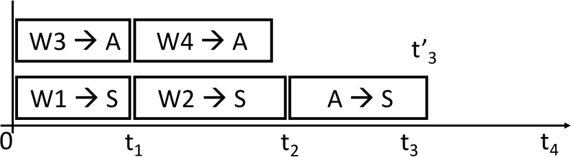
(a) Updates forwarded directly to server

(b) Update forwarded to server through aggregator

Figure 2: Example highlighting advantages of gradient aggregation

In-network control enables the above ordered updates that are ready to be sent to the server to be further opportunistically aggregated at network locations before being applied at the server. Thus, network load is lowered, and model updates occur faster (at earlier times) w.r.t. not aggregating in-network.

Say at time $t=0$ updates ($g_{1},..,g_{4}$) from 4 different workers are available. If all the updates are transferred to the server directly in a time shared manner, completion times are as shown in fig. 2. Even though the update from worker $w_{3}$ is available at $t_{0}$, it is queued and starts transmitting only at $t_{2}$ (after update from $w_{2}$ has completed).

With in-network control, say updates $g_{1}$ and $g_{2}$ are forwarded directly to the server, but $g_{3}$ and $g_{4}$ are aggregated at $A$ (fig. 2). Our aggregation algorithm in §5.2 constructs such aggregation topologies dynamically based on current network load. Assuming full-bisection bandwidth, $g_{3}$ and $g_{4}$ will be transferred concurrently with $g_{1}$ and $g_{2}$. After aggregation, the result $r$ can be transferred to the server, where it updates the model at $t^{\prime}_{3}<t_{4}$.

Since $|r|<|g_{3}|+|g_{4}|$, server network load is reduced. Also, pull requests at time $t\geq t^{\prime}_{3}$ can be replied with fresh information of all 4 model updates; without aggregation, pull requests within $[t^{\prime}_{3},t_{4}]$ don’t capture the last update.

3.3 Toward Bounded Consistency Replication

In PS-based systems, the server stores the entire model. It is therefore crucial to ensure server fault-tolerance. Existing PS implementations use chain replication for fault tolerance [32], which incurs $O(k)$ data overhead for $k$ replicas. They attempt to reduce the data overhead by aggregating updates at the server and forwarding them to the replica once every $n$ iterations. However, if updates are sparse, infrequent replication only amortizes the server data overhead since the total data transferred from server to replica is not reduced.

To reduce server load, we can enable a replication strategy based on workers forwarding a copy of each update directly to the replica. However, such worker-based replication is not easy to achieve without active in-network control. In particular, having workers replicate by themselves fundamentally cannot preserve the ordering of updates. Coupled with the stateful nature of model updates (eqn. 2), this can result in unbounded server-replica model divergence, which makes recovery from the replica slow, if not impossible. We show this next. Then, we discuss how in-network control helps.

Assume at time $t=0$, the server and the replica contain identical models (i.e., $\mathbf{w}^{s}_{0}=\mathbf{w}^{r}_{0}=\mathbf{w}_{0}$) and have the same prior update ($h^{0}$). Let $u_{1},u_{2}$ be the next two updates to the model at the server; assume the same updates are applied in a different order ($u_{2},u_{1}$) at the replica. Then, by applying eqn. 2 twice, the model at server and replica can be computed as:

$$\mathbf{w}^{s}_{2} = \mathbf{w}_{0}+(\gamma h^{0}+u_{1})+\{\gamma(\gamma h^{0}+u_{1})+u_{2}\}$$

$$\mathbf{w}^{r}_{2} = \mathbf{w}_{0}+(\gamma h^{0}+u_{2})+\{\gamma(\gamma h^{0}+u_{2})+u_{1}\}$$ (5)

Thus, the divergence is:

$$\mathbf{w}^{s}_{2}-\mathbf{w}^{r}_{2} = \gamma(u_{1}-u_{2})$$

$$||\mathbf{w}^{s}_{2}-\mathbf{w}^{r}_{2}||_{2} = \gamma||u_{1}-u_{2}||_{2}$$ (6)

Each such re-ordering of updates will add a further non-zero divergence between the server and replica!

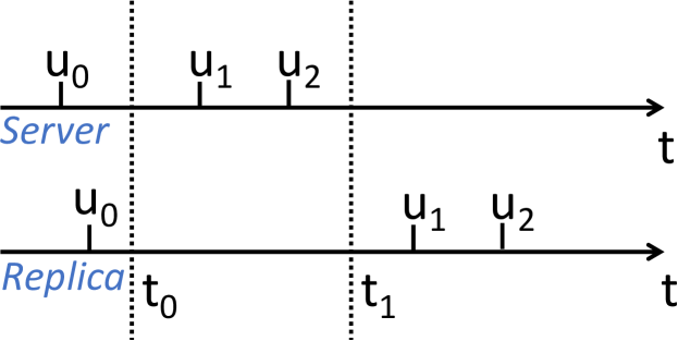
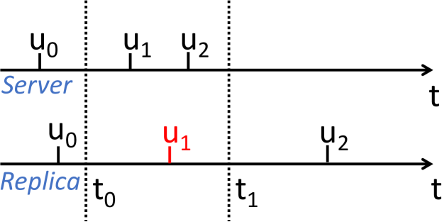
(a) Replica lags the server by two updates

(b) $u_{1}$ scheduled ahead at replica to satisfy divergence bound

Figure 3: Update transfer schedule at server and replica

Enforcing bounded consistency: Using in-network control, we can ensure that all updates to the model at the server are also applied to model at the replica in the exact same order. If the same updates are always applied at the server and replica, then their models are identical, realizing strict consistency. However, we can use in-network control to bound model-replica divergence, thereby leading to a flexible new notion of bounded consistency: here, we simply ensure that $||\mathbf{w}_{s}-\mathbf{w}_{r}||_{2}$ is within a user-specified bound, $Div_{max}$. Bounded consistency flexibly trades off the cost of recovery against network efficiency of updates to primary and replica models. Specifically, a large $Div_{max}$ bound allows delaying several replicated updates, which can be aggressively aggregated later, controlling network replication load. A small bound makes recovery fast but at the cost of higher replication load.

In-network control enables us to carefully schedule both original and replicated updates to achieve bounded consistency. We now show how in-network control can reduce divergence, which we use in our replication algorithm (§5.3),

Consider a scenario where at time $t=0$, update $u_{0}$ is the latest to be applied to the model at both the server and replica; the divergence at $t=t_{0}$ is zero. Now, consider a schedule of future updates $u_{1},u_{2}$ as shown in fig. 3. At time $t=t_{1}$, the server leads the replica by two updates. By applying eqn. 2 twice, the model divergence at $t=t_{1}$ can be computed as:

$$||w^{s}_{2}-w_{0}||_{2}=||(\gamma+\gamma^{2})h^{0}+(1+\gamma)u_{1}+u_{2}||_{2}$$ (7)

where, $h^{0}=w_{0}-w^{-1}$ is the update history at time $t=t_{0}$.

If $||w^{s}_{2}-w_{0}||>Div_{max}$, then we can alter the schedule to reduce the server’s lead over the replica (e.g., fig. 3). With the example new schedule, divergence at time $t=t_{1}$

$$||w^{s}_{2}-w^{s}_{1}||_{2}=||\gamma^{2}h^{0}+\gamma u_{1}+u_{2}||_{2}$$ (8)

is lower than divergence without network control. Our replication algorithm in §5.3 uses this lead reduction idea.

4 Architecture and APIs

Architecture: The main component of MLfabric is a scheduler that interacts with MLfabric daemons on each worker/server; the scheduler processes update and model transfer requests from the daemons and determines the (a) next hop, and (b) schedule for each transfer. The next hop can either be a final destination (worker or server) or an intermediate aggregator deployed alongside workers; aggregators compute the (weighted) sum of incoming updates and forward them to the next hop determined by the scheduler. A network monitor periodically measures and reports available network bandwidth to the scheduler which is used to make scheduling decisions. MLfabric daemons are responsible for interfacing with application entities using MLfabric APIs and enforcing the scheduler’s decisions.

	MLFabric APIs
	registerAsWorker(params)
worker	push(server, update, update_norm)
	get(server, model)
	AllReduce(update)
	registerAsServer(params)
server	registerUpdateCallback()
	registerRequestCallback()
replica	registerAsReplica(server, params)
	registerUpdateCallback()
params	delay bound := $\tau_{max}$
	divergence bound := $Div_{max}$

Table 1: Items in red are extensions we make to the PS API.

APIs: MLfabric extends existing PS APIs (see Table 1). It also provides an MPI AllReduce API which is realized through PS APIs (§6). These APIs help realize the optimizations discussed in §3. For example, for bounded consistency replication (§3.3), MLfabric allows machines to register as replicas and allows workers to specify the norm of the update when it is pushed.

5 Algorithms

MLfabric scheduler determines the communication pattern for a batch of updates available from workers. It computes the transfer schedule (i.e., how bytes in an update are transferred at any given time) and forwarding (next hop – i.e., server or intermediate aggregator hop) for each of these updates. This is done so as to (1) minimize the average completion time of update transfers (§3.1.1), improve network efficiency (§3.2), and make fresh models available earlier (§3.1.1 and §3.2), while (2) bounding worst-case delay (§3.1) even under stragglers or changing network conditions. Also, when replica servers are deployed, MLfabric schedules minimal replication traffic to bound primary-replica model divergence (§3.3).

We first formulate an integer linear program (ILP) to jointly determine the optimal schedules of updates and forwarding for aggregation (§10.1). But the ILP is intractable even for a PS-system with one server and no replicas. It is intractable even when determining the schedules alone (i.e., aggregation is also ignored) while considering delay bounds.

To handle this intractability, we decompose the problem and solve it progressively. As mentioned earlier, we process a batch of updates at a time. We first determine ordering for the batch of updates. Second, given ordering, we determine the forwarding/aggregation strategy, which results in tentative schedules for transferring updates to either servers or aggregators. Third, given the ordering, and schedules of updates, we determine which replica transfers to schedule and when so that they finish before updates in the batch are committed at the server; if this replication “falls short”, i.e., causes server-replica model divergence, we delay a small number of the tentative primary server transfer schedules such that divergence bound is met. In the end, we have concrete transfer schedules for all updates in the batch and for those that are replicated. For simplicity we assume a single server $S$. We describe the above three algorithms in turn.

In : $U$ (Updates), $NW$ (Network state), $S$ (server) Out : $\mathcal{O}(U)$ (Ordered updates) 1 Fn ShrtUp($UU$, $NW$)   // $t_{en}$: As described in fig. 4 2  $g^{*}\leftarrow\mathop{\mathrm{argmin}}\limits_{g\in UU}~{}t_{en}(g,NW,S)$ 3  4  return $g^{*}$ 5  $\mathcal{O}(U)\leftarrow[\quad]$ 6  for $i\leftarrow 1$ to $|U|$ do 7   $g^{*}\leftarrow~{}$ShrtUp($U-\mathcal{O}(U)$, $NW$) 8   $\mathcal{O}(U)\leftarrow[\mathcal{O}(U),\quad g^{*}]$    // NetUp: See fig. 4 9   $NW\leftarrow~{}$NetUp $(NW,g^{*},S)$ 10   end for Algorithm 1 (a)

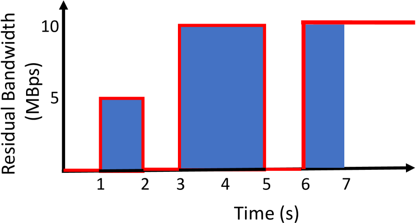
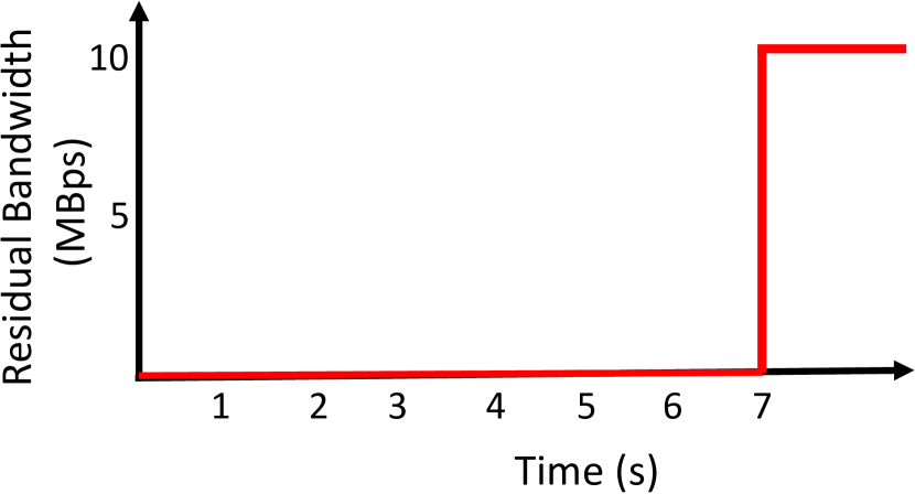
(b)

(c)

Figure 4: Ordering available updates. (a) Shortest transfer first ordering pseudo-code. (b)$t_{en}$ calculation. Consider an update, $g$, of size $30$ MB, available at time $t=0$. The red line represents residual bandwidth along the path for $g$. The blue shaded region represents the bandwidth utilized by update, $g$. Here, $t_{en}(g)=7$. (c) Network b/w update. Residual bandwidth after reserving bandwidth for $g$.

5.1 Update Ordering

Given a set of available worker updates ($U$), and a single server, we first describe how we determine the order ($\mathcal{O}(U)$) in which updates are transferred over the network. We ignore replication/aggregation for now.

We assume network time-sharing (§3.1.1), i.e., updates transferred on a bottleneck link do not have overlapping transfer times. Given this, we attempt to determine an ordering that (1) minimizes the average update transfer time to the server to ensure a fast rate of updates (§3.1.1), (2) subject to the constraints that delays bounds are met. Since this problem in itself is also intractable, we develop a heuristic that decouples them by first attempting to minimize average transfer time (§5.1.1), and then “fixing” any violated delay bounds (§5.1.2). This heuristic may result in network links/server NIC laying “fallow”, and we show how to alter the ordering to address this inefficiency without violating delay bounds (§5.1.3).

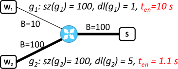
Figure 5: A case for preemptively dropping updates. Update $g_{1}$ takes $10$ s to complete because of low bandwidth behind worker $w_{1}$.

5.1.1 Average completion time

To determine an order that minimizes average update transfer time, we iteratively emulate shortest-job-first ordering for update transfers (alg. 1): in each iteration, given current available bandwidth, we compute each single update’s transfer completion time, $t_{en}$, by factoring in the bottleneck bandwidth the transfer has available over time, and determining how the bytes in the update are transferred by maximally using bottleneck capacity at any time (fig. 4). We pick the transfer with least completion time, and reserve capacity on its path over time; the amount of reservation equals the time-varying bottleneck bandwidth, and reservation duration equals the transfer completion time. We then update remaining network capacities over time, and iterate (line 1, alg.1).

5.1.2 Bounding delays

Shortest-transfer-first-ordering can increase delay (potentially greater than the configured upper bound, $\tau_{max}$) for large updates or those with less bandwidth to the server. To ensure that these are transferred earlier in the order so as to meet delay bounds, we introduce transfer deadlines. For an ordering $\mathcal{O}(U)$ over updates in $U$, the deadline for update $g\in U$ is:

$$dl(g):=v(g)+\tau_{max}-v_{init}$$ (9)

where, $v(g)$ is the model version for update $g$ and $v_{init}$ is the version of the model after all updates from previous batchs are applied.

We then modify the update ordering algorithm (alg. 1) as follows: in iteration $i$ if there exists an unscheduled $g\in U$, such that $dl(g)=i$, then we pick $g$ in that iteration and reserve bandwidth for transferring $g$ as above; otherwise we greedily pick the update with the least transfer time ($t_{en}$).

5.1.3 Dropping delayed updates

Unfortunately, simply accounting for shortest-transfer-first and deadlines does not suffice in determining a “good” ordering. Unless care is taken while factoring deadlines, the ordering may unnecessarily lead to network or server resources staying fallow. To see why, consider two workers $w_{1}$ and $w_{2}$ with updates $g_{1}$ and $g_{2}$. Let the deadline for the two updates be $dl(g_{1})=1$ and $dl(g_{2})=5$. Let the network topology and current state of the network be as shown in fig. 5. Since $g_{1}$ has a deadline of 1, the above approach picks $g_{1}$ as the first update to apply to the model, and thus transfers it first. Because its bottleneck bandwidth is 10Mbps, the transfer would take 10s. In the next iteration, the algorithm selects $g_{2}$. If $g_{2}$ is scheduled immediately, then its available bandwidth is 90Mbps (after bandwidth for $g_{1}$ is reserved), and the update takes 1.1s to finish. Thus, $t_{en}(g_{1})>t_{en}(g_{2})$, which violates $g_{1}$’s delay bound (recall $dl(g_{1})=1$). One way to avoid this is to transfer $g_{2}$ in a delayed manner such that $g_{1}$ is applied first, but this leaves 90Mbps of network capacity on the link to the server unused while only $g_{1}$ is being transferred. Alternately, $g_{2}$ can be transferred per the above ordering, but applied only after $g_{1}$ is applied – in this case the server stays idle while waiting for $g_{1}$ even though $g_{2}$ is available to be applied.

To ensure work conserving server and network behavior as well as delay bounds, we modify our algorithm to drop the update $g_{1}$ at the worker itself. $g_{2}$ is then immediately scheduled for transfer.

In : $U$ (Available updates), $NW$ (Network state), $S$ (server)

Out : $\mathcal{O}(U)$ (Ordered updates)

1 Fn ShrtDline($it$, $UU$, $NW$)

2  $g^{*}\leftarrow~{}$ if $\exists g:dl(g)=it$ then  $g$

3  else  ShrtUp($UU$,$NW$)

4 

5  return $g^{*}$

  $P\leftarrow\phi$

   // processed updates

6  for $i\leftarrow 1$ to $|U|$ do  $dl(g_{i})=v(g_{i})+\tau_{max}-v_{init}$

7  for $i\leftarrow 1$ to $|U|$ do

8   $g^{*}\leftarrow~{}$ ShrtDline $(i$, $U-P$, $NW)$

9   $P\leftarrow~{}P~{}\cup~{}g^{*}$

10   $g^{\circ}\leftarrow~{}$ ShrtDline $(i+1$, $U-P$, NetUp $(NW,g^{*},S))$

11   if $t_{en}(g^{*},NW,S)>t_{en}(g^{\circ},$ NetUp $(NW,g^{*},S),S)$ then  continue

12   $\mathcal{O}(U)\leftarrow[\mathcal{O}(U),\quad g^{*}]$

13   $NW\leftarrow~{}$NetUp $(NW,g^{*},S)$

14   end for

Algorithm 2 Final update ordering algorithm

Thus, our iterative algorithm requires the following fix: in every iteration of the modified algorithm from §5.1.2, where we pick an update (call it “current”) to satisfy a deadline, we look-ahead and determine the completion time of the next update that will be applied (call it “next”). If “next” completes before “current”, we discard “current”. The final ordering algorithm that combines shortest-job-first, meets delay bounds, and avoids wasting resources is in Alg. 2.

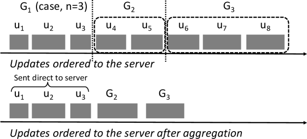
Figure 6: Partitioning ordered updates to server. Later partitions are aggregated before being sent to server. $G_{i}$ are the groups. The figure depicts the case where first 3 updates are sent directly to the server. Note that $u_{6}$ is not added to $G_{2}$ since time taken to aggregate $u_{4},u_{5},u_{6}$ would exceed the time taken to send $u_{1},u_{2},u_{3}$ to the server.

5.2 Aggregation

With the transfer order determined, we describe how to opportunistically aggregate updates in-network. The goal is to use spare compute and network capacity at non-server (aggregator) locations to aggregate as efficiently as possible while preserving the above-determined ordering.

We achieve this by grouping ordered updates in a clever manner, and streaming each group to either the server directly, or first to an aggregator and then the server, such that the server always has a constant stream of ordered or ordered+aggregated updates arriving at its NIC (fig. 6). In some more detail, given a set of $k$ aggregators for the server, we partition ordered updates to the server into $k+1$ groups, using an algorithm we describe shortly. Given the partitioning, the first of these groups, if non-zero in size, is forwarded directly to the server. All gradients in subsequent groups are aggregated before they are forwarded to the server (fig. 6). Further, updates in each group are forwarded to aggregators as per $\mathcal{O}(U)$ determined above. Thus we ensure that, (a) the delay constraints remain satisfied (fig. 6), and (b) update to the model is consistent to the case with no aggregation. The output from the aggregator also obeys the same order.

Our algorithm for determining the best way to partition updates into $k+1$ groups for the server is key to efficiency and is shown in Alg. 3. The algorithm determines group membership so as to minimize the total time until the aggregated update from the last $(k+1)^{st}$ group is transferred to the server. The partitioning is guided by the following key constraint: aggregating all updates in the $i^{th}$ group from the corresponding workers should not finish later than the time when all prior $i-1$ groups’ gradient aggregates are transferred to the server. This condition ensures efficiency, i.e., the server NIC is never left fallow, waiting for updates to be aggregated.

We first randomly pre-assign the aggregator to use for the $i^{th}$ group. Then, the aggregation algorithm works are follows. Given $|U|$ ordered updates, we exhaustively enumerate $|U|+1$ cases (lines 21-23). In the $n^{th}$ such case, $n=0,\ldots,|U|$: (1) the first $n$ updates are forwarded directly to the server (lines 3-7). (2) We greedily assign successive updates to the first aggregator as long as the above-mentioned constraint is satisfied (lines 16-18). (3) When the constraint is violated, we greedily start assigning updates to the second aggregator (lines 10-15), and so on. Figure 6 shows this for $n=3$.

Input : $\mathcal{O}(U)$ (ordered updates), $NW$ (network), $S$ (server)

Output : $A(g),\forall g\in\mathcal{O}(U)$ (aggregator for update, $g$)

1 Fn DetAgg $(n,\mathcal{O}(U),NW,A)$

  $aid~{}\leftarrow~{}0,\quad t_{max}=0$

   // $aid=0$ indicates fwding to server

2  for $i~{}\leftarrow~{}1$ to $n$ do

3   $A(g_{i})~{}\leftarrow~{}aid$

   $t_{max}~{}\leftarrow~{}t_{en}(g_{i},NW,S)$

    // Update time until server is blocked

   $NW~{}\leftarrow~{}$NetUp $(NW,g_{i},S)$

    // Reserve bandwidth for direct transfer to server

4  

5   end for

6  $aid~{}\leftarrow~{}aid+1$,  $i~{}\leftarrow~{}n+1$

7   while $i\leq|\mathcal{O}(U)|$ do

8    if $t_{en}(g_{i},NW,aid)>t_{max}$ then

     $t_{max}~{}\leftarrow~{}t_{en}(a_{aid},NW,S)$

      // $a_{aid}$: aggregated update at $aid$

     $NW~{}\leftarrow~{}$NetUp $(a_{aid},NW,S)$

      // Reserve bandwidth from $aid$ to server

9     $aid~{}\leftarrow~{}aid+1$

10     continue

11     end if

12    $A(g_{i})~{}\leftarrow~{}aid$

     $NW~{}\leftarrow~{}$NetUp $(g_{i},NW,aid)$

      // Reserve bandwidth to aggregator, $aid$

     $i~{}\leftarrow~{}i+1$

      // Consider next update in order

13    

14     end while

15    

16     return $t_{max}$

    /* Enumerate all cases and store aggregation pattern and total time. */

17     for $i~{}\leftarrow~{}0$ to $|\mathcal{O}(U)|$ do

18      DetAgg $(i,\mathcal{O}(U),NW,A)$

19      end for

$i^{*}~{}\leftarrow~{}\mathop{\mathrm{argmin}}\limits_{i\in[0,|\mathcal{O}(U)|]}$ DetAgg $(i,\mathcal{O}(U),NW,A)$

Algorithm 3 Aggregation algorithm.

After every assignment of an update to server/aggregator, we reserve network bandwidth for the transfer (lines 5, 6, 17). We also reserve bandwidth for transferring the aggregated update from the aggregator to the server (lines 11, 12).

All $|U|+1$ cases result in a different aggregation patterns. We pick the one which takes the least amount of time to transfer all the updates to the server (line 24).

Note that our algorithm does not alter the transfer schedules for updates in group 1 compared to those computed by Alg. 2. For all other updates, and aggregates, our algorithm computes new transfer schedules that differ from Alg. 2, because the schedule now accounts for new transfer destinations (aggregators vs. the server) and new transfers/sources (aggregates from aggregators vs. original updates from workers).

We now have transfer schedules for a batch $U$ where: delay bounds are met; updates are aggregated efficiently; updates/aggregates are committed as fast as possible to the server ensuring high model update rate; and server NIC and overall network efficiency are high.

5.3 Replication

Given the above transfer schedules for a batch, we now describe our replication algorithm. It determines the final schedules for transfers to both the server and the replica; thus, we refer to the above-determined schedules (alg. 2) as “tentative”.

Suppose there is just one replica (extending to more replicas is simple). The goal is to transfer a prefix of the $|U|$ updates to replica in the same order as $\mathcal{O}(U)$ (determined above), such that when all the updates in the batch are committed at the server the divergence bound is satisfied. We assume a separate $k^{\prime}$ aggregators are earmarked for the replica.

The replication algorithm operates in cognizance of the above “tentative server schedules” and the resulting network state. It first computes “tentative replica schedules” using the aggregation alg. 3, where the initial state of the network accounts for tentative server (original transfer) schedules.

Suppose the last transfer to finish in the tentative server schedules finished (i.e., committed at the server) at de $T_{last}$. We check if the divergence bound, $Div_{max}$, holds at $T_{last}$ based on the server and replica updates that would have been committed by this time; we can determine this from tentative server and replica schedules as shown shortly. Note that only a prefix of $U$ server updates would have completed by $T_{last}$.

If the bound is satisfied, we freeze the replica schedule (i.e., apply to replica) for all worker-to-aggregator and aggregator-to-replica transfers that would have finished by $T_{last}$; all replicated updates that finish after $T_{last}$ are “punted” to be processed along with the next batch.

If the divergence bound is not satisfied at $T_{last}$, then we delay (akin to the example in (§3.3) just the last update in the tentative server schedule to start after completion of the earliest update in the replica schedule (say, $a_{e}$) such that the divergence bound is satisfied; all replica updates until $a_{e}$ are then frozen (this is still a prefix of $U$); subsequent updates are punted to the next batch.

Punting the processing of some replicated updates to the next batch has two advantages for said next batch: (1) punted transfers combine with the set of replicated updates for said batch, which helps increases overall aggregation efficiency in transfers to the replica when said batch is processed, and, (2) in turn, this helps free up resources for server update transfers in said batch, helping them to finish faster. With a large divergence bound, more such updates are punted to subsequent batches, magnifying the aforementioned benefits. We show this empirically in §7.

Thus, we now have concrete schedules for both server and replica updates.

We return to the problem of efficiently estimating the divergence between sets of updates in the tentative server and replica schedules. Because computing exact divergence requires expensive computation over large updates, in MLfabric, we approximate actual divergence by an upper bound. Suppose at any time, the latest updates to the server and replica are, $w^{2}_{s}$ and $w^{0}$ respectively (see eq. 7). The divergence can be approximated using Cauchy-Schwartz inequality as:

$$||w^{2}_{s}-w^{0}||_{2} = ||(\gamma+\gamma^{2})h^{0}+(1+\gamma)u_{1}+u_{2}||_{2}$$

$$\leq \{a_{1}||h^{0}||^{2}_{2}+a_{2}||u_{1}||^{2}_{2}+a_{3}||u_{2}||^{2}_{2}$$

$$a_{4}||h^{0}||.||u_{1}||+a_{5}||u_{1}||.||u_{2}||$$

$$+a_{6}||u_{1}||.||h^{0}||\}^{\frac{1}{2}}$$

$$= ||w_{s}^{2}-w^{0}||_{2}^{approx.}$$ (11)

where, $h^{0}$ is the update history and $a_{1},\ldots,a_{6}$ are constants dependent on momentum $\gamma$. The value $||w_{s}^{2}-w^{0}||_{2}^{approx.}$ (denoted as $div(s,r)$) can be easily computed with just the norm of the individual updates provided by the workers/server to the MLfabric scheduler (§4); verifying that the approximation is less than $Div_{max}$ is sufficient for bounded consistency.

6 Extending MLfabric

We now describe how MLfabric applies to synchronous and stale synchronous SGD, and to MPI frameworks.

Synchronous SGD/PS: Here, at each iteration, workers read the latest model and compute a local update using a portion of the mini-batch. The updates are then aggregated at the server and applied to the model (also incrementing model version) before the start of next iteration. MLfabric’s approach to construct dynamic network-aware aggregation topologies naturally helps synchronous SGD. The workers’ updates for an iteration are batched when they become ready, say into $|U|$ updates in a batch. Since update ordering does not apply to synchronous SGD, aggregation here starts with a list of updates (vs. an ordering in §5.2). Then, directly applying our algorithm from §5.2 ensures that this batch of updates is transferred as efficiently as possible. The next batch may use a different aggregation topology. Our replication algorithm (§5.3) also applies directly. Note that we have to guarantee bounded divergence only at the end of an iteration (after all workers’ updates are applied) as opposed to end of a batch.

Stale Synchronous SGD/PS: Stale synchronous (SS) SGD is a consistency model that allows slow workers to lag behind fast workers by up to $K$ iterations [23]; typically $K\sim 2$. This form of delay management in SS is restrictive compared to the delay management that MLfabric enables for asynchronous SGD. For example, with $K=2$, the maximum staleness of a model is bound by $2\times num\_workers$. However, a worker that is more than twice slower than other workers will halt progress of all other workers until the slow worker progresses to the next iteration. In contrast, a delay bound of $2\times num\_workers$ in asynchronous SGD with MLfabric will not halt other workers’ progress, while at the same time ensuring the staleness of the update is less than $2\times num\_workers$.

Further, a typical implementation of SS does not implement update aggregation. In-network control offered by MLfabric can be applied to update aggregation for SS in a manner similar to synchronous/PS above.

MPI: MLfabric’s AllReduce API can be used by existing MPI-based systems to implement synchronized SGD. Internally, MLfabric would implement AllReduce through successive calls to: (a) push(root, update, norm) and (b) get(root, update), using a synchronous consistency model; root is randomly chosen among the workers and acts as the root of the aggregation topology, which is a dynamically constructed tree (similar to synchronous/PS above). get(root, update) pulls the aggregated update from root once updates from all workers are received.

MLfabric can also help with model distribution (§10.3).

7 Evaluation

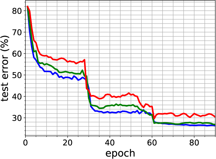
(a) Deeplearning - #iter vs error rate	(b) Deeplearning - time vs error rate	(c) LDA - #iter vs log-likelihood	(d) LDA - time vs log-likelihood

Figure 7: MLfabric vs state-of-the-art approaches for asynchronous and synchronous LDA and Deep learning

Implementation: MLfabric is implemented in C++ as a thin communication control layer between DML applications (e.g., PLDA [25], Keras [11], Tensorflow [6]) and MPI communication libraries (OpenMPI [18] and NCCL [2]). DML applications interact with MLfabric through APIs defined in Table 1 and MLfabric internally uses APIs provided by MPI frameworks to aggregate/schedule transfers across the network.

Datasets and ML models: We evaluate MLfabric with two popular communication intensive distributed ML applications: (1) distributed deep learning for image recognition on the ImageNet1K [17] data set (using ResNet50 and ResNet152 [20] models), and, (2) distributed LDA for topic modelling using Gibbs sampling on the NY Times dataset [3]. The computation and communication structure of distributed LDA is similar to SGD; instead of computing a gradient update using a mini-batch, each worker computes a numerical update to a word-topic matrix using its entire shard of data, and then exchanges the update among all the workers [25] using a PS or MPI based system.

Experiment setup: We run the DML applications across 30 workers in a cluster of 15 baremetal machines connected by a 10 Gbps network. The worker computation for distributed LDA runs on a 4-core CPU with 2.3GHz processor whereas the deep learning applications use NVIDIA P100 GPUs (2 cards/physical machine).

The scheduler, server (single) and replica (single) are hosted on a dedicated machine with $10$Gbps bandwidth. The aggregators are co-hosted with worker clients; the aggregator runs on a separate core on the worker machines and does not compete for CPU resources. We batch requests at the scheduler every $100ms$.

Background compute and network load: Along the lines of prior work [24], we emulate compute stragglers by slowing down the update computation stage; a single worker has an $r$% chance of being slowed down by a factor of $s$; by default, $(r,s)=(10,2)$ (compute setting C1). We also study other settings; C2: $(r,s)=(10,4)$ and C3: $(r,s)=(4,2)$.

We emulate network background traffic by varying the rate limits on physical hosts’ NICs; incoming and outgoing links are treated independently. For every $T$ (= 5, default) seconds the NIC rate is changed to a value from the set $\{1,2.5,3.3,5,10\}$ Gbps with probability $p=\{p_{1},p_{2.5},p_{3.3},p_{5},p_{10}\}$; it emulates the case where there are $\{9,3,2,1,0\}$ other contending flows respectively ($p=\{0,0,0,0.1,0.9\}$ is the default settings, called N1). We also consider two other settings; N2:$(0,0.1,0.1,0.1,0.7)$ and N3:$(0.5,0,0,0,0.5)$.

The network monitor reports changes in link bandwidth to the scheduler after $t_{lag}$ (= 0.2s, default).

Algorithms: We evaluate the following: PS-based asynchronous and synchronous variants of MLfabric, or MLfabric-A & MLfabric-S, respectively; vanilla PS-based asynchronous (Async); and MPI-based (using NCCL library) synchronous algorithms – we study two variants, ring-reduce and tree-reduce, or RR-Sync and Tr-Sync, respectively.

7.1 Performance of MLfabric-A

We compare MLfabric-A with $Async$ and RR-Sync. We also study the effect of varying delay.

Distributed deep learning: Figures 7- 7 plot the top-1 test error (in %) for a ResNet50 model (100 MB) trained on the ImageNet1K dataset as a function of training epochs and time respectively (for the setting C1-N1). We use a mini-batch size of 32 per worker and a learning rate schedule that reduces by a factor of 10 after epochs 30, 60, and 90. We compare MLfabric-A only with RR-Sync; the communication bottleneck at the parameter server for $Async$ is prohibitive to run even over a few days.

With a delay bound of 30, MLfabric-A-30, can train a deep neural network with 74% accuracy; it alleviates server bottleneck through update aggregation. The convergence rate as function of number of epochs is similar to RR-Sync.

In terms of wall clock time MLfabric-A-30 is $1.74\times$ faster than RR-Sync. The speed up can be attributed to: (1) asynchronous algorithms are not prone to compute stragglers, (2) unlike synchronous algorithms, MLfabric-A does not have to send traffic over low bandwidth links in each iteration; update from workers behind slow links can be dropped. During the entire training process, MLfabric-A-30 dropped 30% of the updates at the worker for violating delay bounds.

We comment on the impact of delay control. A higher delay bound than the 30 used above can reduce the number of dropped updates and speed up the training time at the cost of loss in accuracy. MLfabric-A-60, with a delay bound of 60, achieves only 70% test accuracy; however, it is $1.36\times$ times faster than RR-Sync. We also experimented with an intermediate delay (45) and saw that it’s accuracy and run-time lie between delay-30 and delay-60.

	NS1	NS2	NS3
CS1	1.74	1.23	1.42
CS2	2.96	2.0	2.32
CS3	1.90	1.33	1.42

Table 2: Speedup in time w.r.t RR-Sync

Varying compute and network settings: Next, we varied CS and NS settings to evaluate the benefits of MLfabric-A for different kinds of heterogenuous environments. Table 2 shows the speedup of MLfabric-A relative to RR-Sync across 9 different compute and network background loads. Here, to minimize the overall running time, we start with a pre-trained model (i.e., the model after epoch 50 for synchronous SGD). The run time is measured as time taken to reach 74% test accuracy.

Speed-up is highest (3X) when some workers are $4\times$ slower than others (C2) and the network is not the bottleneck (N1). This is because in RR-Sync AllReduce is triggered only after receiving update-ready notification from all workers. Thus, in the presence of stragglers, network bandwidth remains fallow waiting for a slow worker to compute the update.

Varying reporting lag: For network settings N2, increasing the reporting lag up to 2s (from 0.2s, with the network re-configured every 5 seconds) increases the per-iteration time averaged over 10 epochs (for ResNet50) by 100ms–7.6% of overall 1300ms. However, for a skewed distribution of link bandwidths, $p_{1}=0.2$ and $p_{10}=0.8$, the per-iteration time increased by 40% with a 2s lag. Thus, the gains from MLfabric are robust to lags in monitoring unless bandwidth skews are significant.

Distributed LDA: Figures 7 and 7 compares performance of RR-Sync, Async and MLfabric-A based on the number of iterations and time taken to converge for the topic modelling task using NY times dataset (vocabulary size=102660, number of documents=300K); we use compute setting C1 and network setting N1 for this experiment. We learn a model with 100 topics; the model is said to have converged when the log-likelihood reaches -7.94 on a test data of size 1500. RR-Sync, MLfabric-A-30, MLfabric-A-60 and Async converge in 145 (182s), 188 (139s), 239 (169s) and 300 (1080s) iterations (wall clock time) respectively. This corresponds to a $1.6\times$ and $1.25\times$ speedup (in number of iterations) for MLfabric in comparison to Async for with delay bounds 30 and 60 respectively. Further, even though MLfabric-A takes more number of iterations, it reduces the overall run time w.r.t RR-Sync by 24% and 7% for delays 30 and 60. Due to update aggregation, MLfabric is up to $7\times$ faster than Async. Similar gains were obtained for other compute and network settings.

Importance of delay control and aggregation: Our results above show the relative importance of these two aspects of MLfabric. They show that MLfabric’s aggregation plays a crucial role in supporting all large model training; without it, training is prohibitively slow. Note that MLfabric enables aggregation for the first time for asynchronous algorithms. Delay control is also important, because without it either accuracy (ResNet-50) or runtime (LDA) are impacted.

7.2 Performance of MLfabric-S

We compare the performance of MLfabric-S (using ResNet50) with RR-Sync for different compute and network settings. We measure the overall time to complete 5 epochs for both the algorithms. We find that the bandwidth optimal RR-Sync is faster ($1.2-2\times$) than MLfabric-S for all combinations of compute and network settings except C2 and N1. When some workers are slowed down by a factor of $4$, then for the C2-N1 setting, the rest of the workers are idle (no computation or communication) for 50% of the overall runtime. For all other settings, communication generally is not idle. MLfabric-S reduces the idle time by eagerly aggregating available worker updates (even over low bandwidth links). This results in a 16% improvement in overall run time in C2-N1. For ResNet-152 model (240MB) with the above compute and network settings, RR-Sync is the optimal algorithm since communication is always the bottleneck.

Figure 8: Histogram of number of update messages sent over links with different bandwidths.

Figure 9: Reduction in data sent to replica as function of $Div_{max}$ (K)

We also compare MLfabric-S with another (non-bandwith optimal) variant of MPI AllReduce (Tr-Sync) that aggregates and distributes updates along a binary tree. In the presence of stragglers (C2) and network contention (N2), MLfabric-S reduces the per-iteration communication time for ResNet-152 by 21.7%: from 3.05s with Tr-Sync to 2.38s. For ResNet-50 the gain is 18.42%. Clearly, the advantages of network-aware aggregation are more prominent for larger model sizes. Since compute time is relatively small, the reduction in per-iteration time directly translates to reduction in overall running time of the algorithm for large models. The benefits arise from dynamically avoiding (aggregating more) updates at nodes with low (high) current bandwidth; figure 9 plots the number of updates aggregated as a function of the bandwidth available on the incoming link. Note that since Tr-Sync uses a binary tree the number of messages exchanged between workers is higher. However, being network-aware, MLfabric-S forwards only 816 of the overall 20000 (3%) messages to aggregators with low bandwidth (2.5Gbps in N2), whereas Tr-Sync sends 1800 messages over such links!

7.3 Bounded consistency replication

For MPI based systems, fault tolerance is provided today by checkpointing the model at the worker with rank 0. We compare the cost of checkpointing with the cost of transferring updates to a hot-standby replica over the network. We measure the overhead of fault-tolerance as follows: for MPI based systems the overhead is the difference in time between two runs with and without checkpointing over 6 epochs ($\approx 20$ minutes with no stragglers/network bottlenecks). For PS based systems, it is the time difference between two runs with and without in-network replication. The runs with fault tolerance are parameterized by the maximum allowable divergence (measured in number of updates) between server and replica; for MPI systems it translates to checkpointing frequency. The overhead of checkpointing for every iteration and every 20 iterations is 76 minutes and 4 minutes, respectively, for MPI based systems; the corresponding overhead for in-network replication is 16 mins and 10 mins, respectively. As the divergence bound increases (600 updates in the case of 20 iterations), the network cost savings due to aggregation plateaus at a factor of $5.6$ for 30 workers (see fig. 9). Further, if all workers only write part of their model to disk every iteration and replicate it 3-way, the 76 minute overhead can be reduced to just $7$ minutes. Thus, overall, in-network replication does not help with MPI based systems.

For PS based DML systems running asynchronous SGD, checkpointing at the server for every 30 and 600 updates has an overhead of 96 minutes (6X worse w.r.t. in-network replication) and 6 minutes (0.6X), respectively. Thus, in-network replication is advantageous over checkpointing here for scenarios that warrant tight divergence bound (e.g., where compute nodes are highly susceptible to failure).

Chain replication is commonly used in many PS frameworks. We also experimented with it, but found that, given the large model sizes, it adds prohibitive overhead (up to 30X) compared to in-network replication in MLfabric.

7.4 Scheduler performance

For our experimental setting with 30 workers, the transfer schedules were computed within $5$ ms per batch (batch size, $|U|$, is typically $<10$). To test scalability of the scheduler computation, we studied the effect of varying sizes of $|U|$. We measure the time taken by the scheduler to determine the concrete batch schedules by providing batches of $|U|$ updates (with random deadlines from $Uniform(1,2|U|)$) for a network topology with $|U|/2$ nodes and a congestion free core. For update batch sizes of 100, 500 and 1000, the scheduler overhead was $30$ ms, $440$ ms, and $1460$ ms, respectively. Thus, the overhead is quadratic w.r.t. update batch size. However, we note that the inner loops in alg. 2 (line 3, function ShrtUp) and 3 (lines 21-23) can be parallelized (which our current implementation does not), leading to better scaling.

8 Related work

Prior works propose various techniques to reduce the overall training time of ML algorithms that employ SGD for learning.

Algorithmic approaches: Some other approaches for mitigating stragglers involve: aggregating gradients from only a subset of fast workers in each iteration of synchronous SGD [16], which is complementary with MLfabric’s aggregation; and delay-aware learning rate for asynchronous SGD [31], which can benefit from MLfabric’s delay management. Prior work advocates variance reduction SGD where a series of asynchronous updates is interspersed with intermediate synchronous updates [16], and performing partial updates of the model to reduce total data sent over the network [33, 22]; both techniques can benefit from MLfabric.

System-level approaches: To speed up gradient computation time, ML systems leverage SIMD processing capabilities of hardware accelerators like GPU or TPU [6], which can leverage MLfabric for further speedup. Communication overhead is typically managed by: (1) workers leveraging sparsity of data and pulling only parts of the model [23], or (2) quantization of floating point values used to represent gradients [30]. MLfabric is complementary with #1 and #2.

Our overall approach can be view as type of co-flow [12, 14, 13, 28, 36] scheduling. The differences in our setting are: (1) flows in our co-flow have an intrinsic order, (2) we can drop/re-order flows from the co-flow, (3) flows in our co-flow can be aggregated in-network using ML algorithm specific aggregation functions. These aspects make our problem markedly difficult and different.

9 Conclusion

We designed MLfabric, a communication library for speeding up large-scale distributed machine learning (DML) systems in dynamic cluster settings. We showed that fine-grained in-network control helps MLfabric to (1) algorithmically speed up convergence, (2) improve network efficiency via dynamic update aggregation, and (3) offload model replication responsibilities from servers to the network in a network-efficient manner. Our experiments on a 30-worker GPU cluster using real-world datasets and realistic straggler settings show that MLfabric reduces model training time by up to $3\times$ compared to state-of-the-art algorithms. Finally, this work does not raise any ethical issues.

10 Appendix

10.1 ILP formulation for joint ordering and forwarding for aggregation

Let $W=\{w_{1},..,w_{n}\}$ be the workers and $S$ be the server storing a DML application’s model. Let, $A=\{a_{1},..,a_{\ell}\}$ be the aggregators that serve as intermediate hops. Let $G=(V,E)$ denote a directed graph representing the underlying communication network. $V$ is the set of all hosts and switches and $E$ is the set of network links including host to switch links. Let $B(e),\forall e\in E$ denote the capacity of link $e$. We assume the path, $P(v_{1},v_{2})$, from $v_{1}$ to $v_{2}$ over the set of links $E$ is fixed and does not change in time. Different paths can share a network link.

To exploit dynamic aggregation and re-ordering, we jointly determine the schedule for a batch of requests; let $U=\{g_{1},\ldots,g_{|U|}\}$ denote a batch of ready updates.

Variables: Let the variable $r_{g_{i}}(t)$ denote the rate at which update $g_{i}$ is transmitted by $w_{i}$ over time. Modeling the rate as a function of time allows us to capture network time sharing and ordering between updates. E.g., if updates $g_{1}$ and $g_{2}$ from $w_{1}$ and $w_{2}$ have to time-share a link $e$ such that $w_{1}$ sends data first followed by $w_{2}$, the rate for $g_{1}$ and $g_{2}$ are:

$$r_{g_{1}}(t)=\begin{cases}B(e),&\text{if}\quad 0\leq t<\frac{sz(g_{1})}{B(e)}\\ 0,&\text{otherwise}\end{cases}$$ (12)

$$r_{g_{2}}(t)=\begin{cases}B(e),&\text{if}\quad\frac{s(g_{1})}{B(e)}\leq t<\frac{sz(g_{1})+sz(g_{2})}{B(e)}\\ 0,&\text{otherwise}\end{cases}$$ (13)

Here, $sz(g)$ is the update size. Update ordering hinges on start/end times:

$$t_{st}(g_{i}) = \{\text{min}(t):r_{g_{i}}(t)>0\}$$ (14)

$$t_{en}(g_{i}) = \{\text{max}(t):r_{g_{i}}(t)>0\}$$ (15)

$g_{1}$ is applied before $g_{2}$ if $t_{en}(g_{1})<t_{en}(g_{2})$.

Let the integer variable $dst(g_{i})$ denote the immediate next hop for $g_{i}$; since a worker can forward the update either to the server or an aggregator, $dst(g_{i})\in\{S\}\cup A$. We also determine the schedule of aggregated updates. Let $r_{a_{j}}(t)$ be the rate at which $a_{j}$ forwards the aggregated update to the server and let $t_{st}(a_{j})$ and $t_{en}(a_{j})$ represent the start/end times.

Objective: For synchronous SGD, we have:

$$\text{obj}_{sync}:=\max\left(\max_{\begin{subarray}{c}g\in U\\ dst(g)=s\end{subarray}}t_{en}(g),\quad\max_{a\in A}~{}~{}t_{en}(a)\right)$$ (16)

This minimizes the total time to aggregate all updates in $U$. For asynchronous SGD, we optimize the average completion time per update:

$$\text{obj}_{async}:=\frac{1}{|U|}\left(\displaystyle\sum\limits_{\begin{subarray}{c}g\in U\\ dst(g)=s\end{subarray}}t_{en}(g)+\displaystyle\sum\limits_{a\in A}m(a)t_{en}(a)\right)$$ (17)

where, $m(a)$ is the number of updates aggregated at $a$. Further, $t_{en}(g),\forall g\in U$, should be such that delay bounds are satisfied.

Modeling the destination for each update ($dst(g)$), rate of transfer at each discrete point in time ($r_{g}(t)$) results in an large number of discrete variables. Solving an ILP with large number variables is time-wise expensive and is not a straight forward choice for the low-latency requirements at the scheduler. Thus, MLfabric breaks down the complex ILP into smaller sub-problems (ordering, aggregation, replication) and develops computationally efficient heuristics to solve them.

10.2 Model split across multiple servers

Our algorithms in §5 considered the case of a single parameter server; we now briefly describe the case where the model is split across a set $S$ of servers. Thus, $g_{i}$, from a worker consists of $|S|>1$ components, $g_{i}=\{g_{i}^{1},\ldots,g_{i}^{|S|}\}$. All the components of $g_{i}$ are computed from the same version of the model and thus, will have the same deadline. Below, we ignore aggregation and replication and consider just scheduling (§5.1) for simplicity; the modifications we suggest below naturally apply to algorithms for replication (§5.3) and aggregation (§5.2).

One option to schedule updates to multiple servers is to use an algorithm similar to one described in §5.1.2 by defining deadlines for each individual server and update component. For example, consider two updates, $g_{1}=[g_{1}^{1},g_{1}^{2}]$ and $g_{2}=[g_{2}^{1},g_{2}^{2}]$, to two destination servers, $s_{1}$ and $s_{2}$. By treating all the updates as independent and choosing them in a shortest transfer first order we might reserve network resources in the following order $g_{1}^{1}\rightarrow g_{2}^{1}\rightarrow g_{1}^{2}\rightarrow g_{2}^{2}$, if updates to $s_{1}$ are small in size. In the presence of a large number of workers, this would result in some parts of the model being updated less frequently than others.

To ensure uniform number of updates to all components of the ML model, network resources for all update components are reserved together. In each iteration of our algorithm, we pick the update which has the largest completion time for all its components:

$$t_{en}(g)=\max_{j}~{}t_{en}(g^{j})$$ (18)

10.3 Model distribution

Aggregating updates reduces overall runtime by reducing the amount of data forwarded to the server. However, if each request for the model is responded to individually then the down-link at the server will become the bottleneck. To reduce the load on the down-link, we use a distribution tree for propagating the model to the workers. At the server, requests are batched and responded with same version of model. The distribution pattern is determined similar to the aggregation pattern. For a batch of requests, $k^{\circ}$ distributors are earmarked. Mapping of workers to distributors is done using a variant of alg. 3 obtained by replacing $t_{en}()$s as the times taken to transfer the model from server-to-distributor and distributor-to-worker. Once the partitioning is determined, we first transfer the model from the server to the $k^{\circ}$-th distributor and then proceed backwards. The workers in the first group receive the model directly from the server.

10.4 SGD convergence analysis under bounded delay

We extend the proof of convergence under uniform delay from [31]. Specifically, we modify Lemma A.3, under the assumption that delay is uniform in: $\tau_{t,\epsilon}\sim\textrm{Uniform}({\bar{\tau}-\epsilon,\bar{\tau}+\epsilon})$. We bound the delay dependent term $\Delta(t,\epsilon)$ (see A.15 in [31], also defined below) under the new delay model.

$$\Delta(t,\epsilon):=\frac{1}{2\alpha\big{(}t,\tau(t,\epsilon)\big{)}}\big{[}||x^{*}-x_{t}||^{2}-||x^{*}-x_{t+1}||^{2}\big{]}$$ (19)

We then show that,

$$\sum_{t=1}^{T}\mathbb{E}[\Delta(t,\epsilon)]\leq\frac{1}{2}(L+c)R^{2}+\mathcal{O}(\epsilon\sqrt{T-\epsilon})$$ (20)

The expected loss after $T$ iterations can then be bounded as (see Corollary 3.2 in [31]):

$$E[L(\mathbf{w}_{T})]-L(\mathbf{w}^{*})\leq\frac{1}{t}\sum_{t=1}^{T}\mathbb{E}[\Delta(t,\epsilon)]\leq\frac{1}{T}\mathcal{O}(\epsilon\sqrt{T-\epsilon})\quad\quad\hfill$$

Proof: Let $r_{t}=||x_{t}-x^{*}||^{2}$, observe that it is not independent of $\tau(t-1,\epsilon)$. Thus, with

$$z_{t,\epsilon}=\frac{1}{\alpha\big{(}t,\tau(t,\epsilon)\big{)}}-\frac{1}{\alpha\big{(}t-1,\tau(t-1,\epsilon)\big{)}}=c\Big{(}\sqrt{t+\tau(t,\epsilon)}-\sqrt{t-1+\tau(t-1,\epsilon)}\Big{)}$$ (21)

we have

$$\sum_{t=1}^{T}\mathbb{E}[\Delta(t,\epsilon)]=\mathbb{E}\bigg{[}\sum_{t=1}^{T}\Delta(t,\epsilon)\bigg{]}=\frac{1}{2}\mathbb{E}\bigg{[}\frac{r(1)}{\alpha\big{(}1,\tau(1,\epsilon)\big{)}}+\sum_{t=1}^{T}z_{t,\epsilon}r_{t}\bigg{]}\leq\frac{1}{2}(L+c)R^{2}+\frac{1}{2}\mathbb{E}\bigg{[}\sum_{t=2}^{T}z_{t,\epsilon}r_{t}\bigg{]}$$ (22)

$$\mathbb{E}[z_{t,\epsilon}r_{t}]=\mathbb{E}_{\tau_{t,\epsilon}}\big{[}\mathbb{E}[z_{t,\epsilon}r_{t}|\tau_{t,\epsilon}]\big{]}=\frac{1}{2\epsilon+1}\sum_{l=\bar{\tau}-\epsilon}^{\bar{\tau}+\epsilon}\bigg{(}\sum_{s=\bar{\tau}-\epsilon}^{l-1}\frac{r_{t,s}c}{2\epsilon+1}\Big{(}\sqrt{t+l}-\sqrt{t-1+s}\Big{)}\bigg{)}$$ (23)

Consider the inner summation, we have

$$\frac{cR^{2}\sum_{s={\bar{\tau}-\epsilon}}^{l-1}(l-s+1)}{(2\epsilon+1)\sqrt{2(t+\bar{\tau}-\epsilon)-1}}=\frac{cR^{2}(\bar{\tau}-\epsilon+l)(l+3+\bar{\tau}-\epsilon)}{2\cdot(2\epsilon+1)\sqrt{2(t+\bar{\tau}-\epsilon)-1}}$$ (24)

Thus, we now consider

$$\mathbb{E}[z_{t}r_{t}] \leq\frac{1}{2\epsilon+1}\sum_{l=\bar{\tau}-\epsilon}^{\bar{\tau}+\epsilon}\frac{cR^{2}(\bar{\tau}-\epsilon+l)(l+3+\bar{\tau}-\epsilon)}{2\cdot(2\epsilon+1)\sqrt{2(t+\bar{\tau}-\epsilon)-1}}$$

$$=\frac{cR^{2}}{2\cdot(2\epsilon+1)^{2}\sqrt{2(t+\bar{\tau}-\epsilon)-1}}\sum_{l=\bar{\tau}-\epsilon}^{\bar{\tau}+\epsilon}(\bar{\tau}-\epsilon+l)(l+3+\bar{\tau}-\epsilon)$$

Since

$$\sum_{l=\bar{\tau}-\epsilon}^{\bar{\tau}+\epsilon}(\bar{\tau}-\epsilon+l)(l+3+\bar{\tau}-\epsilon)=\frac{2}{3}(2\epsilon+1)(9\bar{\tau}+6\bar{\tau}^{2}-4\epsilon-6\bar{\tau}\epsilon+2\epsilon^{2})$$ (25)

$$\mathbb{E}[z_{t}r_{t}] =\frac{cR^{2}(9\bar{\tau}+6\bar{\tau}^{2}-4\epsilon-6\bar{\tau}\epsilon+2\epsilon^{2})}{3\cdot(2\epsilon+1)\sqrt{2(t+\bar{\tau}-\epsilon)-1}}<\frac{cR^{2}(9\bar{\tau}+6\bar{\tau}^{2})}{3\cdot(2\epsilon+1)\sqrt{2(t+\bar{\tau}-\epsilon)-1}}+\frac{cR^{2}(-4\epsilon-6\bar{\tau}\epsilon+2\epsilon^{2})}{3\cdot 2\epsilon\sqrt{2(t+\bar{\tau}-\epsilon)-1}}$$

$$=\frac{cR^{2}(9\bar{\tau}+6\bar{\tau}^{2})}{3\cdot(2\epsilon+1)\sqrt{2(t+\bar{\tau}-\epsilon)-1}}-\frac{cR^{2}(4\epsilon+6\bar{\tau}\epsilon)}{3\cdot 2\epsilon\sqrt{2(t+\bar{\tau}-\epsilon)-1}}+\frac{cR^{2}2\epsilon^{2}}{3\cdot 2\epsilon\sqrt{2(t+\bar{\tau}-\epsilon)-1}}$$

$$<\frac{cR^{2}(9\bar{\tau}+6\bar{\tau}^{2})}{3\cdot 1\sqrt{2(t+\bar{\tau}-\epsilon)-1}}-\frac{cR^{2}(2+3\bar{\tau})}{3\cdot\sqrt{2(t+\bar{\tau}-\epsilon)-1}}+\frac{cR^{2}\epsilon}{3\cdot\sqrt{2(t+\bar{\tau}-\epsilon)-1}}$$

$$=\frac{cR^{2}(6\bar{\tau}+6\bar{\tau}^{2}-2)}{3\sqrt{2(t+\bar{\tau}-\epsilon)-1}}+\frac{cR^{2}\epsilon}{3\sqrt{2(t+\bar{\tau}-\epsilon)-1}}$$

Finally,

$$\mathbb{E}\bigg{[}\sum_{t=2}^{T}z_{t,\epsilon}r_{t}\bigg{]}=\sum_{t=2}^{T}\mathbb{E}[z_{t,\epsilon}r_{t}]\leq\int_{1}^{T}\frac{cR^{2}(6\bar{\tau}+6\bar{\tau}^{2}-2)}{3\sqrt{2(t+\bar{\tau}-\epsilon)-1}}+\frac{cR^{2}\epsilon}{3\sqrt{2(t+\bar{\tau}-\epsilon)-1}}\mathrm{d}t=\mathcal{O}(\epsilon\sqrt{T+\bar{\tau}-\epsilon})$$ (26)

References

- [1] Caffe2: A new lightweight, modular, and scalable deep learning framework. https://caffe2.ai/.
- [2] NVIDIA Collective Communication Library. https://github.com/NVIDIA/nccl. Accessed: 2018-01-01.
- [3] NY Times Dataset. https://archive.ics.uci.edu/ml/machine-learning-databases/bag-of-words.
- [4] PyTorch -Distributed communication package. http://pytorch.org/docs/master/distributed.html.
- [5] Tensors and Dynamic neural network in Python with strong GPU accleration. http://pytorch.org/.
- [6] Abadi, M., Barham, P., Chen, J., Chen, Z., Davis, A., Dean, J., Devin, M., Ghemawat, S., Irving, G., Isard, M., Kudlur, M., Levenberg, J., Monga, R., Moore, S., Murray, D. G., Steiner, B., Tucker, P., Vasudevan, V., Warden, P., Wicke, M., Yu, Y., and Zheng, X. Tensorflow: A system for large-scale machine learning. In 12th USENIX Symposium on Operating Systems Design and Implementation (OSDI 16) (GA, 2016), USENIX Association, pp. 265–283.
- [7] Agarwal, A., and Duchi, J. C. Distributed delayed stochastic optimization. In Advances in Neural Information Processing Systems 24, J. Shawe-Taylor, R. S. Zemel, P. L. Bartlett, F. Pereira, and K. Q. Weinberger, Eds. Curran Associates, Inc., 2011, pp. 873–881.
- [8] Blei, D. M., Ng, A. Y., and Jordan, M. I. Latent dirichlet allocation. Journal of machine Learning research 3, Jan (2003), 993–1022.
- [9] Bottou, L., Curtis, F. E., and Nocedal, J. Optimization Methods for Large-Scale Machine Learning. ArXiv e-prints (June 2016).
- [10] Chen, T., Li, M., Li, Y., Lin, M., Wang, N., Wang, M., Xiao, T., Xu, B., Zhang, C., and Zhang, Z. Mxnet: A flexible and efficient machine learning library for heterogeneous distributed systems. CoRR abs/1512.01274 (2015).
- [11] Chollet, F., et al. Keras. https://keras.io, 2015.
- [12] Chowdhury, M., and Stoica, I. Coflow: A networking abstraction for cluster applications. In HotNets (2012).
- [13] Chowdhury, M., and Stoica, I. Efficient coflow scheduling without prior knowledge. In SIGCOMM (2015).
- [14] Chowdhury, M., Zhong, Y., and Stoica, I. Efficient coflow scheduling with varys. In Proceedings of the 2014 ACM Conference on SIGCOMM (New York, NY, USA, 2014), SIGCOMM ’14, ACM, pp. 443–454.
- [15] Cui, H., Zhang, H., Ganger, G. R., Gibbons, P. B., and Xing, E. P. Geeps: Scalable deep learning on distributed gpus with a gpu-specialized parameter server. In Proceedings of the Eleventh European Conference on Computer Systems (New York, NY, USA, 2016), EuroSys ’16, ACM, pp. 4:1–4:16.
- [16] Dean, J., Corrado, G. S., Monga, R., Chen, K., Devin, M., Le, Q. V., Mao, M. Z., Ranzato, M., Senior, A., Tucker, P., Yang, K., and Ng, A. Y. Large scale distributed deep networks. In NIPS (2012).
- [17] Deng, J., Dong, W., Socher, R., Li, L., Li, K., and Fei-Fei, L. Imagenet: A large-scale hierarchical image database. In 2009 IEEE Conference on Computer Vision and Pattern Recognition (June 2009), pp. 248–255.
- [18] Graham, R. L., Woodall, T. S., and Squyres, J. M. Open mpi: A flexible high performance mpi. In Parallel Processing and Applied Mathematics (Berlin, Heidelberg, 2006), R. Wyrzykowski, J. Dongarra, N. Meyer, and J. Waśniewski, Eds., Springer Berlin Heidelberg, pp. 228–239.
- [19] Gu, J., Chowdhury, M., Shin, K. G., Zhu, Y., yeongjae Jeon, Qian, J., Liu, H., and Guo, C. Tiresias: A gpu cluster manager for distributed deep learning. In Symposium on Networked Systems Design and Implementation (NSDI 19) (2019).
- [20] He, K., Zhang, X., Ren, S., and Sun, J. Deep residual learning for image recognition. In 2016 IEEE Conference on Computer Vision and Pattern Recognition (CVPR) (June 2016), pp. 770–778.
- [21] Ho, Q., Cipar, J., Cui, H., Kim, J. K., Lee, S., Gibbons, P. B., Gibson, G. A., Ganger, G. R., and Xing, E. P. More effective distributed ml via a stale synchronous parallel parameter server. In Proceedings of the 26th International Conference on Neural Information Processing Systems (USA, 2013), NIPS’13, Curran Associates Inc., pp. 1223–1231.
- [22] Kim, J. K., Ho, Q., Lee, S., Zheng, X., Dai, W., Gibson, G. A., and Xing, E. P. STRADS: a distributed framework for scheduled model parallel machine learning. In Proceedings of the Eleventh European Conference on Computer Systems, EuroSys 2016, London, United Kingdom, April 18-21, 2016 (2016), pp. 5:1–5:16.
- [23] Li, M., Andersen, D. G., Park, J. W., Smola, A. J., Ahmed, A., Josifovski, V., Long, J., Shekita, E. J., and Su, B.-Y. Scaling distributed machine learning with the parameter server. In 11th USENIX Symposium on Operating Systems Design and Implementation (OSDI 14) (Broomfield, CO, Oct. 2014), USENIX Association, pp. 583–598.
- [24] Lian, X., Zhang, W., Zhang, C., and Liu, J. Asynchronous decentralized parallel stochastic gradient descent. In International Conference on Machine Learning (2018).
- [25] Liu, Z., Zhang, Y., Chang, E. Y., and Sun, M. Plda+: Parallel latent dirichlet allocation with data placement and pipeline processing. ACM Transactions on Intelligent Systems and Technology, special issue on Large Scale Machine Learning (2011). Software available at https://github.com/openbigdatagroup/plda.
- [26] Nocedal, J., and Wright, S. J. Numerical optimization (2nd edition), 2006.
- [27] Peng, Y., Bao, Y., Chen, Y., Wu, C., and Guo, C. Optimus: An efficient dynamic resource scheduler for deep learning clusters. In Proceedings of the Thirteenth EuroSys Conference (New York, NY, USA, 2018), EuroSys ’18, ACM, pp. 3:1–3:14.
- [28] Qiu, Z., Stein, C., and Zhong, Y. Minimizing the total weighted completion time of coflows in datacenter networks. In SPAA (2015).
- [29] Recht, B., Re, C., Wright, S., and Niu, F. Hogwild: A lock-free approach to parallelizing stochastic gradient descent. In Advances in Neural Information Processing Systems 24, J. Shawe-Taylor, R. S. Zemel, P. L. Bartlett, F. Pereira, and K. Q. Weinberger, Eds. Curran Associates, Inc., 2011, pp. 693–701.
- [30] Seide, F., Fu, H., Droppo, J., Li, G., and Yu, D. 1-bit stochastic gradient descent and application to data-parallel distributed training of speech dnns. In Interspeech 2014 (September 2014).
- [31] Sra, S., Yu, A. W., Li, M., and Smola, A. J. Adadelay: Delay adaptive distributed stochastic optimization. In AISTATS (2016).
- [32] van Renesse, R., and Schneider, F. B. Chain replication for supporting high throughput and availability. In Proceedings of the 6th Conference on Symposium on Opearting Systems Design & Implementation - Volume 6 (Berkeley, CA, USA, 2004), OSDI’04, USENIX Association, pp. 7–7.
- [33] Wei, J., Dai, W., Qiao, A., Ho, Q., Cui, H., Ganger, G. R., Gibbons, P. B., Gibson, G. A., and Xing, E. P. Managed communication and consistency for fast data-parallel iterative analytics. In Proceedings of the Sixth ACM Symposium on Cloud Computing (New York, NY, USA, 2015), SoCC ’15, ACM, pp. 381–394.
- [34] Xiao, W., Bhardwaj, R., Ramjee, R., Sivathanu, M., Kwatra, N., Han, Z., Patel, P., Peng, X., Zhao, H., Zhang, Q., Yang, F., and Zhou, L. Gandiva: Introspective cluster scheduling for deep learning. In Proceedings of the 12th USENIX Conference on Operating Systems Design and Implementation (Berkeley, CA, USA, 2018), OSDI’18, USENIX Association, pp. 595–610.
- [35] Zhang, J., and Mitliagkas, I. YellowFin and the Art of Momentum Tuning. ArXiv e-prints (June 2017).
- [36] Zhao, Y., Chen, K., Bai, W., Tian, C., Geng, Y., Zhang, Y., Li, D., and Wang, S. RAPIER: Integrating routing and scheduling for coflow-aware data center networks. In INFOCOM (2015).