Influence measures in subnetworks using vertex centrality

Abstract

This work deals with the issue of assessing the influence of a node in the entire network and in the subnetwork to which it belongs as well, adapting the classical idea of vertex centrality. We provide a general definition of relative vertex centrality measure with respect to the classical one, referred to the whole network. Specifically, we give a decomposition of the relative centrality measure by including also the relative influence of the single node with respect to a given subgraph containing it. The proposed measure of relative centrality is tested in the empirical networks generated by collecting assets of the $S\&P$ 100, focusing on two specific centrality indices: betweenness and eigenvector centrality. The analysis is performed in a time perspective, capturing the assets influence, with respect to the characteristics of the analysed measures, in both the entire network and the specific sectors to which the assets belong.

1 Introduction

Complex networks are experiencing an increasing popularity among scientists, either under a methodological as well as practical perspective. They represent a versatile framework for the description of real-world systems with interconnected components (see e.g. Newman (2010), Wasserman and Faust (1994)). In the context of complex networks, a very relevant theme is the assessment of the relevance of the single nodes in the overall structure. In this respect, we mention e.g. Cinelli et al (2017), Cerqueti et al (2018), Ma and Ma (2019) and Wang et al (2011), where the identification of the key actors among the agents is a crucial task for exploring the proposed applied problem – inter organizational innovation, social media and air transportation, respectively.

Widely used instruments for identifying the influence of the single nodes in a complex network are the so-called centrality measures. Such devices compound a set of methodological tools sharing the same target of measuring the relevance of the nodes, with the distinctions due to the declination of the concept of relevance (see e.g. Freeman and Freeman (1979); Perra and Fortunato (2008); Watts (2004)).

Centrality measures are usually defined as absolute quantities, hence providing an objective description of the importance of the individual nodes of the network. Essentially, they can be also presented as normalized terms, so that nodes – also belonging to different networks – can be compared according to their relevance/centrality measure. This universality property of the definition of centrality measures has the severe drawback of not allowing the contextualization of the nodes relevance in the overall network. To fix ideas, think at a node with a very high degree, namely a hub. If such a node belongs to a network with low average degree, then the network is star-shaped and the hub is the crucial node; if, contrastingly, such a node belongs to a network with high average degree, then the considered hub is an important element, but it is not the only one. For instance, the hub can be part of a rich club (see e.g. Cinelli et al (2017, 2018); Colizza et al (2006); Opsahl et al (2008)), i.e. of a proper subset of nodes with high degree, or it can be “one among many”, because even all the other nodes of the network have high degree. All these aspects are not covered by the absolute centrality measures.

Therefore, although traditional centrality measures have been formulated for individual nodes, it is equally interesting to explore the idea of a group centrality. As pointed out in Everett and Borgatti (1999), the group centrality allows to “quantify” the membership of a node to a group. For instance, this could be useful to efficiently remodulate groups, removing internal redundant ties that poorly contribute to the group importance.

According to the arguments above, this paper adds to the debate on centrality measures by proposing two natural advancements to the related theory. First, it provides a general definition of the relative centrality measure of a node with respect to the classical one of the entire network. Second, it offers a decomposition of the relative centrality measure by including also the relative influence of the single node with respect to a given subgraph containing it, hence leading to a concept of group centrality.

One intuitive approach to define a group centrality is to average the centrality scores in the group, but more suitable and effective group centrality measures have been proposed (Everett and Borgatti (1999)). In this work, we consider, in the same formula, the average centrality of nodes in a group and the group centrality defined in the literature. In particular, the comparison between these two values allows to catch the effect of the external vertices to the centrality measure of the nodes belonging to a specific group.

Our final target is then to quantify the importance of a vertex with respect to a subnetwork. This importance will be measured in terms of centrality. In other words, we aim at catching how much a vertex has a central role with respect to both the whole graph and the subgraphs to which the vertex belongs.

In assessing subgraph centrality, we are in line with Estrada and Rodriguez-Velazquez (2005), where the authors propose a characterization of the nodes on the basis of the loops containing them. Such closed walks can be identified with related connected subgraphs, so that their number proxies the relevance of the single nodes over the subgraphs of the network.

We here adopt a different perspective by dealing with a relative measure rather than an absolute one; in this way, our approach allows the comparison of nodes and subgraphs also in presence of different networks.

The theoretical model is validated through empirical experiments based on the daily returns of the components of the $S\&P$ 100 for the period Jan 1st, 2001 - Dec 31st, 2017. A system of networks is considered on the ground of a time windows analysis. The arcs are weighted through the correlation coefficients between couples of assets in the specific time windows and nodes are the assets. The validation is carried out in the context of two specific relative centrality measures: betweenness and eigenvector centrality. The former one gives information on how nodes are relevant in terms of their role in connecting other nodes of the graph, and it has been introduced by Freeman (1977); the latter centrality measure – whose introduction dates back to the end of the nineteenth century, and we refer to Bonacich (1987) – assigns a high power to the nodes connected to highly relevant nodes. We purposely focused on two alternative centrality measures with a different meaning. Both measures overcome the simple degree centrality, that refers exclusively to the node’s neighbours. On one hand, the betweenness score catches how a node is influential in controlling the flow of information along shortest paths in the network. On the other hand, the eigenvector centrality captures influences at long distances. We argue that these differences can seize the hidden role of assets in local communities. Moreover, both measures represent suitable tools for evaluating nodes’ role in large networks. The empirical analysis is carried out in a time perspective, capturing the assets influence, with respect to the characteristics of the analysed measures, in both the entire network and the specific sectors to which they belong. Main results show that such measures are of particular interest in the proposed exercise and offer important insights on the reality of the considered empirical sample.

The rest of the paper is organized as follows. Section 2 outlines the notation used in the paper, with the basic concepts. Section 3 is devoted to the theoretical formalization of the relative centrality of nodes and subgraphs in a very general environment. Section 4 contains the empirical validation of the theoretical model. Such a section is divided in subsections, with the aim of giving a detailed view of the considered dataset, on the specific relative centrality measures employed for the exercise along with some remarks on limitations and comparisons with other measures. Section 5 presents and discusses critically the results of the empirical experiments. Last section offers some conclusive remarks and traces lines for future research.

2 Preliminaries and notations

We now review some theoretical concepts about graphs and networks . Formally, a network is represented by a graph $G=(V,E)$, that is a set of $n$ nodes (vertices) $V$ and $m$ edges $E$ of unordered pairs of vertices. Two nodes are adjacent if there is an edge $(i,j)$ connecting them. $G$ is undirected if $(j,i)\in E$ whenever $(i,j)\in E$. The complete graph $K_{n}$ is the graph in which every pair of distinct vertices is linked by an edge. A $i-j$ path is a sequence of distinct adjacent vertices from vertex $i$ to vertex $j$. The distance $d(i,j)$ between $i$ and $j$ is the length of the shortest path joining them when such a path exists, and it is set to $+\infty$ otherwise. A graph $G$ is connected if there is a path between every couple of vertices. A subgraph $G_{s}=\left(V_{s},E_{s}\right)$ of $G$ is a graph such that $V_{s}\subseteq V$ and $E_{s}\subseteq E$. A particular class of subgraphs is the one of the induced subgraphs. A subgraph $G_{s}=\left(V_{s},E_{s}\right)$ of $G$ is induced by $V_{s}$ when $(i,j)\in E$ implies $(i,j)\in E_{s}$, for each $i,j\in V_{s}$. A maximal connected subgraph of $G$ is called connected component of $G$. A graph is connected if has exactly one connected component.

In general, the adjacency relationships between vertices of $G$ are described by a nonnegative, real $n$-square matrix $\mathbf{A}$ (the adjacency matrix). We denote with $\rho$ its spectral radius and $\mathbf{x}$ the associated eigenvector. If $G$ is connected, then $\mathbf{A}$ is irreducible and, by Perron Frobenius Theorem, all elements of the eigenvector associated with the spectral radius are strictly positive. This eigenvector is called Perron (or principal) eigenvector.

3 Relative centrality of a subgraph

In the following, we assume that $G=(V,E)$ is a connected and undirected graph of $n$ nodes. For our purposes, we exclude the case of complete graph $K_{n}$, as all vertices show in this case the same topological structure.

Centrality is generally defined in terms of a function $c:V\rightarrow[0,+\infty)$, that assigns nonnegative real values to nodes of the set $V$ of a graph such that

$$c(i)\geq c(j)\iff i\>\textnormal{is at least central as}\>j.$$ (1)

Without losing of generality, we assume that centrality measures are normalized, so that $c(i)\in[0,1]$ for each $i\in V$.
According to this condition, we introduce the relative incidence of the centrality of a node $i$ with respect to the average centrality of the graph $G$ (or, simply, relative centrality of $i$ with respect to $G$) as:

$$c(i|G)=\frac{c(i)}{{\bar{c}(G)}}$$ (2)

where ${\bar{c}(G)}=\frac{\sum_{j=1}^{n}c(j)}{n}$ is the average centrality of $G$.

This index allows a direct comparison of the relative centralities of the specific nodes when considering also the overall related graphs.

By means of a relative index we can assess how much a vertex is “relevant” in a network, where the peculiar declination of the concept of relevance depends on the specific centrality measure employed. In a general sense, the centrality of the node is compared with the average centrality of the graph. In this respect, notice that $c(i|G)$ can be lower or higher than $1$, according to its position with respect to the average behaviour of the network.

The total order in (1) can be reproduced also in the relative case, so that

$$c(i|G)\geq c(j|G)\iff i\>\textnormal{is at least relatively central as}\>j.$$ (3)

It is worth noting that this definition does not alter the centrality ranking. Indeed, comparing $c(i|G)$ through order in (3) leads to the same order of comparing $c(i)$ through order in (1).

The definition of $c(i|G)$ in (2) allows to investigate also the role/position of a vertex with respect to both the whole network and any subnetwork having it as a node. Let $G_{s}=\left(V_{s},E_{s}\right)$, be a subgraph of $G$ (where the cardinality of $V_{s}$ is $n_{s}$) which $i$ belongs to. For instance, $G_{s}$ could be the induced subgraph of $n_{s}\leq n$ nodes of $G$. Moreover, assume that there exists $j\in V_{s}$ such that $c(j)>0$.

Then, formula (2) can be rewritten as:

$$c(i|G)=\frac{c(i)}{{\bar{c}(G_{s})}}\frac{\bar{c}(G_{s})}{{\bar{c}(G)}}=c(i|G_{s})r_{G_{s}}$$ (4)

where ${\bar{c}(G_{s})}=\frac{\sum_{j\in V_{s}}c(i)}{n_{s}}$ is the average centrality of $G_{s}$.

Formula (4) highlights two specific components in the relative centrality of a node with respect to the average behaviour of the network:

• $c(i|G_{s})$ is the relative incidence of the centrality of a node with respect to the average behaviour of the considered subnetwork to which the node belongs.

• $r_{G_{s}}$ quantifies how much the average centrality of the considered subnetwork is far from the average behaviour of the network.

In this way, through $c(i|G_{s})$ we catch if the node is relevant in its subnetwork or not; by means of $r_{G_{s}}$ we are able to take into account of the subnetwork position in the whole network. For instance, the disaggregated terms in formula (4) may suggest that a node could be important by itself, because it is essential in conveying information in the network, but it belongs to a group that on average is not relevant with respect to the whole network.
We proceed further disaggregating the factors of the relative centrality measure, to gain more information. Indeed, it could be interesting to measure the importance of a vertex as element of a subgraph, also referring to the centrality of the considered subnetwork. To this end, we introduce an additional component depending on the centrality of the subnetwork $G_{s}$. We will call this component ${c}(G_{s})$ and we rewrite $c(i|G)$ as:

$$c(i|G)=\frac{c(i)}{{c(G_{s})}}\frac{c(G_{s})}{{\bar{c}(G_{s})}}\frac{\bar{c}(G_{s})}{{\bar{c}(G)}}=\frac{c(i)}{{c(G_{s})}}k_{G_{s}}r_{G_{s}}$$ (5)

The term ${c}(G_{s})$ is a measure of the group centrality related to $G_{s}$. Measures of group centrality have been proposed in Everett and Borgatti (1999) for some well-known vertex centralities. We avoid to give a definition of it in the general case, and refer to next subsection where some specific cases of centrality measure $c$ will be presented. This said, we are implicitly assuming that $G_{s}$ is such that ${c}(G_{s})\neq 0$, so that definition (5) is well-posed.

The term $k_{G_{s}}$ quantifies how much the subnetwork centrality is far from the average centrality. An high value of this ratio is typically due to the higher contribute of the external vertices to the centrality measure of the nodes belonging to the group. On other hand, when the structure of the nodes that are outside $G_{s}$ leads to a high vaue of centrality measure, a lower ratio is observed.

4 Empirical experiments on the market network

This section is devoted to the illustration of the usefulness of the relative centrality measure and of its components. As we will see, we present the paradigmatic cases of betweenness and eigenvector centrality applied to financial markets.

4.1 Description of the dataset and construction of the networks

In this section, we test the proposed approaches performing some empirical applications. We collected daily returns of a dataset referred to the time-period ranging from January 2001 to the end of 2017, that includes $102$ leading U.S. stocks constituents of the $S\&P$ 100 index at the end of 2017. Returns have been divided by using monthly stepped two-years windows. More precisely, the data of the first in-sample window of width two years are used to build the first network, therefore the process is repeated rolling the window one month forward until the end of the dataset is reached. We obtain a totality of 181 networks, the first one, denoted as “1-2001”covers the period Jan 1st, 2001 to Dec $31^{nd}$, 2002. The latter one (“1-2016”) covers the period Dec $1^{st}$, 2016 to Dec $31^{nd}$, 2017.
As a result, for each window, we have a network $G_{t}=(V_{t},E_{t})$ (with $t=1,...,181$), where nodes are the assets and edges are weighted by computing the correlation coefficient ${}_{t}\rho_{i,j}$ between each couple of assets. Notice that the number of assets can vary over time. We have indeed considered the 102 assets constituents of the $S\&P$ 100 index at the end of 2017. For some of these assets no information are available in some specific time periods. Therefore, in each window we have considered only assets whose observations are sufficiently large to assure a significant estimation of the correlation coefficient. As a consequence, the number of nodes in the 181 networks varies from 83 to 102 during the time-period.
As already mentioned in the introduction, in the present analysis we filter $G_{t}$ ($t=1,..,181$) considering only the edges whose associated correlation coefficients are larger than $0.3$ (i.e. we obtain, for each time period, a network $G^{F}_{t}=(V_{t},E^{F}_{t})$). This value has been estimated as suggested in Battiston et al (2010) and the approach can be useful to preserve only links associated with statistically significant correlation.
Since the analysis of assets centrality seems a relevant topic in the related literature, by referring to the filtered networks we focus here on the study of the relative importance of an asset with respect to the portfolio of all assets as well as those characterized by assets of the same sector.

4.2 Employed relative centrality measures

We now introduce the relative centrality measures employed in the analysis. Their formalization mirrors the general arguments of Section 3, with some details that are reported for the sake of clarity.

4.2.1 Relative Betweenness Centrality

The shortest-path betweenness centrality (Freeman (1979)) quantifies how often a node is located on a shortest path between all other nodes. Formally, it is the percentage of geodesics between pairs of vertices $j,k\neq i$, passing through $i$:

$$b(i)=\sum_{j<k}\frac{g_{jk}\left(i\right)}{g_{jk}}$$ (6)

where $g_{jk}$ is the number of geodesics from node $j$ to node $k$, and $g_{jk}\left(i\right)$ is the number of those geodesics that pass through $i$. The normalized measure is $\frac{b(i)}{{n-1\choose 2}}$.

Formula (2), applied to the specific case of betweenness centrality, becomes:

$$b(i|G)=\frac{b(i)}{{\bar{b}(G)}}$$ (7)

where ${\bar{b}(G)}=\frac{\sum_{i=1}^{n}b(i)}{n}$ is the average betweenness of $G$.
Let us suppose that $i$ belongs to a subgraph $G_{s}$; then formula (4) is, in this case:

$$b(i|G)=\frac{b(i)}{{\bar{b}(G_{s})}}\frac{\bar{b}(G_{s})}{{\bar{b}(G)}}=b(i|G_{s})r_{G_{s}}$$ (8)

where ${\bar{b}(G_{s})}=\frac{\sum_{i\in G_{s}}b(i)}{n_{s}}$ is the average betweenness of $G_{s}$.

According to the general concept in Section 3, we intend to quantify the intermediary role position of vertex $i$ taking into account also of the centrality of the subnetwork $G_{s}$. As previously said for centrality in general, a measure of betweenness centrality referred to a subset of vertices in a network (the so-called group betweenness centrality) has been introduced by Everett and Borgatti (1999) in a more general context. For convenience of the reader, we remind here the definition. $\forall j,k\in G\setminus G_{s}$, let $g_{jk}(G_{s})$ be the number of $j-k$ geodesic paths passing through at least one vertex of $G_{s}$. The group betweenness centrality of $G_{s}$ is:

$$b(G_{s})=\sum_{j<k}\frac{g_{jk}\left(G_{s}\right)}{g_{jk}},\quad j,k\in G\setminus G_{s}$$ (9)

Group betweenness measures the betweenness of $G_{s}$ only referring to the paths leading to the external vertices, i.e. vertices that do not belong to the subgraph.

According to formula (5), $b(i|G)$ can be rewritten as:

$$b(i|G)=\frac{b(i)}{{b(G_{s})}}\frac{b(G_{s})}{{\bar{b}(G_{s})}}\frac{\bar{b}(G_{s})}{{\bar{b}(G)}}=b^{G}(i|G_{s})k^{b}_{G_{s}}r^{b}_{G_{s}}$$ (10)

Through the previous formula the relative betweenness of a node can be seen with respect to the average behaviour of the network, in three components:

• $b^{G}(i|G_{s})$ measures how much the node $i$ is essential in conveying information with respect to the intermediary role of its subnetwork;

• $k^{b}_{G_{s}}$ quantifies how much the betweenness of the subnetwork is far from the average betweeness. An high value of this ratio is achieved in presence of high contribution to the betweenness of the nodes of $G_{s}$ of the nodes outside $G_{s}$, which means that $G_{s}$ is relevant for conveying information among nodes not belonging to $G_{s}$.

• $r^{b}_{G_{s}}$ quantifies how much the average betweenness of $G_{s}$ is far from the average betweenness of the entire network, hence measuring the discrepancy between $G_{s}$ and $G$ in terms of inner connectivity.

Notice that, the group betweenness centrality definition provided by formula (9) allows $b(G_{s})=0$. We are implicitly assuming that $b(G_{s})\neq 0$ since formula (10) is meaningless otherwise; however, it could be interesting to analyse also the case of $b(G_{s})=0$, to intercept extremal situations. Indeed, some individuals could have a non-zero betweenness centrality although they are member of a subnetwork with zero group betweenness. In this case, we can measure $b(i|G)$ by using formulas (7) and (8), but obviously it does not make sense to evaluate the component $b^{G}(i|G_{s})$.

4.2.2 Relative Eigenvector Centrality

The eigenvector centrality is an extremely important measure of vertex influence in the network. The meaning of this measure stems from the fact that a vertex is highly central if it is adjacent to vertices that are themselves highly central.
In a formal way, the centrality score is defined using the Perron vector $\mathbf{x}$. More precisely, the eigenvector centrality (Bonacich (1972, 1987)) is defined as:

$$x(i)=\frac{1}{\rho}\sum_{j=1}^{n}a_{ij}x(j),$$ (11)

where $\rho$ is the spectral radius of the adjacency matrix $\mathbf{A}$, as explained in Section 2. In this way, not only the number of adjacent nodes contributes to the node centrality, but also their centralities. Since the node centrality is reinforced by the centralities of its neighbours, this measure well captures the power of a vertex in a network. The normalized eigenvector measure is $\frac{\mathbf{x}}{\parallel\mathbf{x}\parallel_{\tiny 2}}$, where $\parallel\mathbf{x}\parallel_{\tiny 2}$ is the Euclidean norm.

Focusing on the eigenvector, formula (2) becomes:

$$x(i|G)=\frac{x(i)}{{\bar{x}(G)}}$$ (12)

where ${\bar{x}(G)}=\frac{\sum_{i\in G}x(i)}{n}$ is the average eigenvector centrality of $G$. Notice that ${\bar{x}(G)}$ never vanishes, since $x(i)\neq 0\>\forall i\in G$.
Formula (4), that highlights the relative centrality with respect to the average centrality of the subgraph, becomes in this case:

$$x(i|G)=\frac{x(i)}{{\bar{x}(G_{s})}}\frac{\bar{x}(G_{s})}{{\bar{x}(G)}}=x(i|G_{s})r^{x}_{G_{s}}$$ (13)

where ${\bar{x}(G_{s})}=\frac{\sum_{i\in G_{s}}x(i)}{n_{s}}$ is the average eigenvector centrality of $G_{s}$.

As already done in Section (4.2.1), we want to provide a measure of the eigenvector centrality of the subnetwork, using a measure of group centrality. The idea is to replace all the nodes of the subnetwork by a single node whose neighbourhood is the union of the neighbourhoods of all subnetwork members. In other words, an edge from the new vertex to another one exists if there is at least one vertex in the subnetwork who had that link. Through this approach, named in the literature “Reduced Model Approach”, we generate a new graph $G^{*}$ (reduced graph) of $n-n_{s}+1$ vertices, of which we can compute the individual centralities in order to obtain the centrality measure for the subset. Using the Reduced Model Approach we can then compute the eigenvector centrality $x(G_{s})$ referred to the subnetwork $G_{s}$. Hence, formula (5) is in this case equal to:

$$x(i|G)=\frac{x(i)}{{x(G_{s})}}\frac{x(G_{s})}{{\bar{x}(G_{s})}}\frac{\bar{x}(G_{s})}{{\bar{x}(G)}}=x^{G}(i|G_{s})k^{x}_{G_{s}}r^{x}_{G_{s}}$$ (14)

Moving to the interpretation, we then extrapolate from (14) the following components:

• $x^{G}(i|G_{s})$ relates the power/influence of the node $i$ with respect to the power of its subnetwork. In other words, it measures the individual power in respect to the collective power. This component gives insights about the fact that the node is powerful “by himself” or its power arises from its group membership;

• $k^{x}_{G_{s}}$ quantifies how much the subnetwork is powerful with respect to the average power;

• $r^{x}_{G_{s}}$ quantifies how much the subnetwork is powerful on average with respect to the entire network.

Notice that, unless the group betweenness measure, the group eigenvector is always greater than zero, given the connectivity assumption on the network $G$.

4.2.3 Some remarks on the selected centrality measures

Further remarks can be made about the choice of the most appropriate centrality measure, namely, the measure that better identifies the idea of being “influential”. As pointed out in the introduction, eigenvector centrality captures influences at long distances. More precisely, whereas degree centrality measures the local influence of a node, the eigenvector centrality captures the global influence. However, although widely used, eigenvector centrality also presents some limitations. Depending on the network structure, most of the weights of the eigenvector could be concentrated in few nodes, like hubs. In this case, most of the nodes will present centrality close to zero and, therefore, the importance of nodes is not well quantified. For instance, Martin et al. (2014) show that, in random networks with only one high-degree hub or power-law degree distributions, the leading eigenvector can undergo a localization in which most of the weight of the vector is concentrated around the hub vertex and its neighbours, whereas the centrality of the remaining nodes vanishes for large networks. Additionally, Landherr et al. (2010) show that eigenvector centrality does not display perfect monotonicity with respect to distance and shortest path. However, an empirical analysis, conducted on the robustness of measures of centrality in the face of random error in the network data, show that four different centrality measures (betweenness, closeness, degree and eigenvector centrality) are surprisingly similar with respect to pattern and level of robustness in random networks (see Borgatti et al. (2006)).
Other centrality measures, in line with this one, have been provided in the literature. Among them, Katz centrality (see Katz (1953)) takes into account short, medium and long range influences, modulated by an attenuation factor $\alpha$. Formally, it is defined as row sums of the matrix $(\mathbf{I}-\alpha\mathbf{A}^{-1})$, that is the sum of the series of $\alpha^{k}\mathbf{A}^{k}$, being $0<\alpha<\lambda_{1}$, where $\lambda_{1}$ is the largest eigenvalue of $\mathbf{A}$. According to Katz, not only the number of direct connections but also the further interconnectedness of nodes plays an important role for the overall interconnectedness in a social network. Therefore, Katz includes all walks of arbitrary length from the considered node to the other nodes of the network, penalizing the contribution of walks of length $k$ by $\alpha^{k}$. Hence, this centrality measure falls in the middle between the local measure (the degree) and the global one (the eigenvector). The selection of the attenuation factor adds another challenge. Different choices of $\alpha$ lead to different node rankings (Benzi (2015)).
However, it is worth pointing out that formula (14) can be also provided for the case of Katz centrality. Indeed, it is possible to compute the Katz centrality of the subnetwork $G_{s}$ by applying the Reduced Model Approach previously described.

5 Results and Discussion

Given the filtered network $G^{F}_{t}=(V_{t},E^{F}_{t})$ (with $t=1,...,181$), derived as described in Section 4.1, we initially computed betweenness and eigenvector centralities, that have been explored by previous works in this field (Pozzi et al (2013), Peralta and Zareei (2016)). In particular, by means of formula (2), the relative incidence for each node and for each measure have been obtained.

At the global level, an interesting result is provided by the behaviour of the standard deviation of the relative nodes’ centrality over time (see Figure 1). Although slight differences, we observe that the standard deviation of both relative centrality measures tends to decrease in period of crisis. Both the financial crisis period in 2007-2008, which is identified with the Lehman Brothers failure, and the Sovereign debt crisis in 2010-2011 are noticeable. This behaviour reflects the fact that the correlation between assets is higher in this period, leading to an increase in the density of the filtered network and then to similar behaviours in terms of centrality between assets. Such an outcome meets the well-known stylized fact in finance, for which assets correlation increases in times of financial distress.

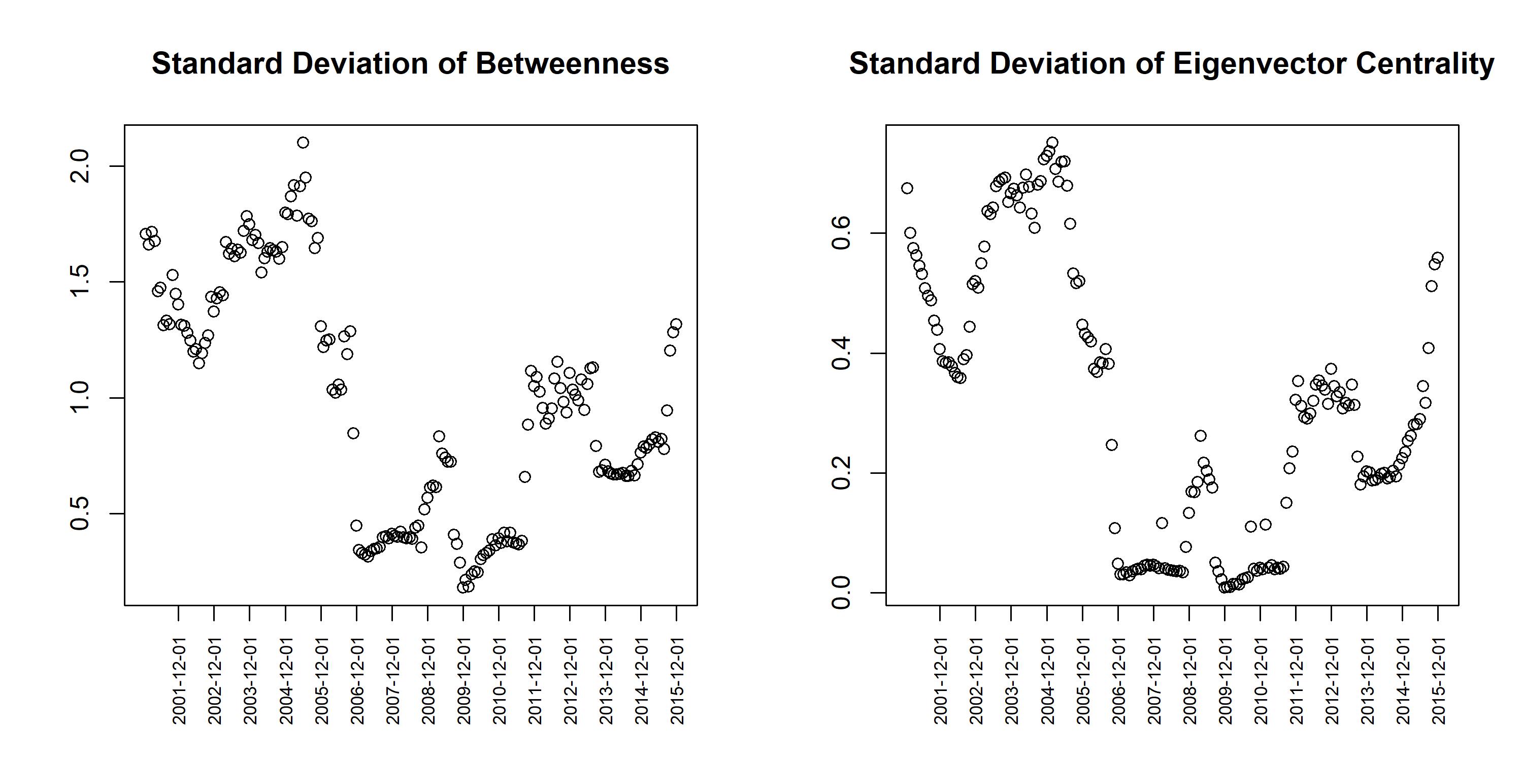
Figure 1: Given the specific filtered network $G^{F}_{t}$ (with $t=1,...,181$), the relative betweenness centrality $b(i|G^{F}_{t})$ of each node $i$ has been computed. The process is repeated for each time period and, for each $t$, we compute the standard deviation of the distribution of the relative centrality measures obtained. Results are displayed on the left side. On the right side, the same procedure has been applied by considering the relative eigenvector centrality $x(i|G^{F}_{t})$.

Concerning specific assets, we report in Figure 2 the networks $G^{F}_{t}$ “1-2007”and “1-2016”. They refer to data of the two-year periods 2007-2008 and 2016-2017, respectively. Assets have been classified in 10 sectors, according to the standard sector classification defined by the Global Industry Classification Standard developed by Morgan Stanley Capital International and Standard & Poor’s. In Figure 2 we relate the size of the nodes to the value of the relative centrality (betweenness for the upper figures and eigenvector for the lower ones). As already stressed, we observe both a higher average centrality and higher differences between assets in quiet periods. Some sectors appear prominent in terms of centrality, also showing a greater homogeneity between nodes. On the contrary, other sectors show a significant heterogeneity, with a few nodes extremely central and several non-central ones (see, for instance, Consumer Staples and Health Care in the “1-2016”network based on relative betweenness centrality).

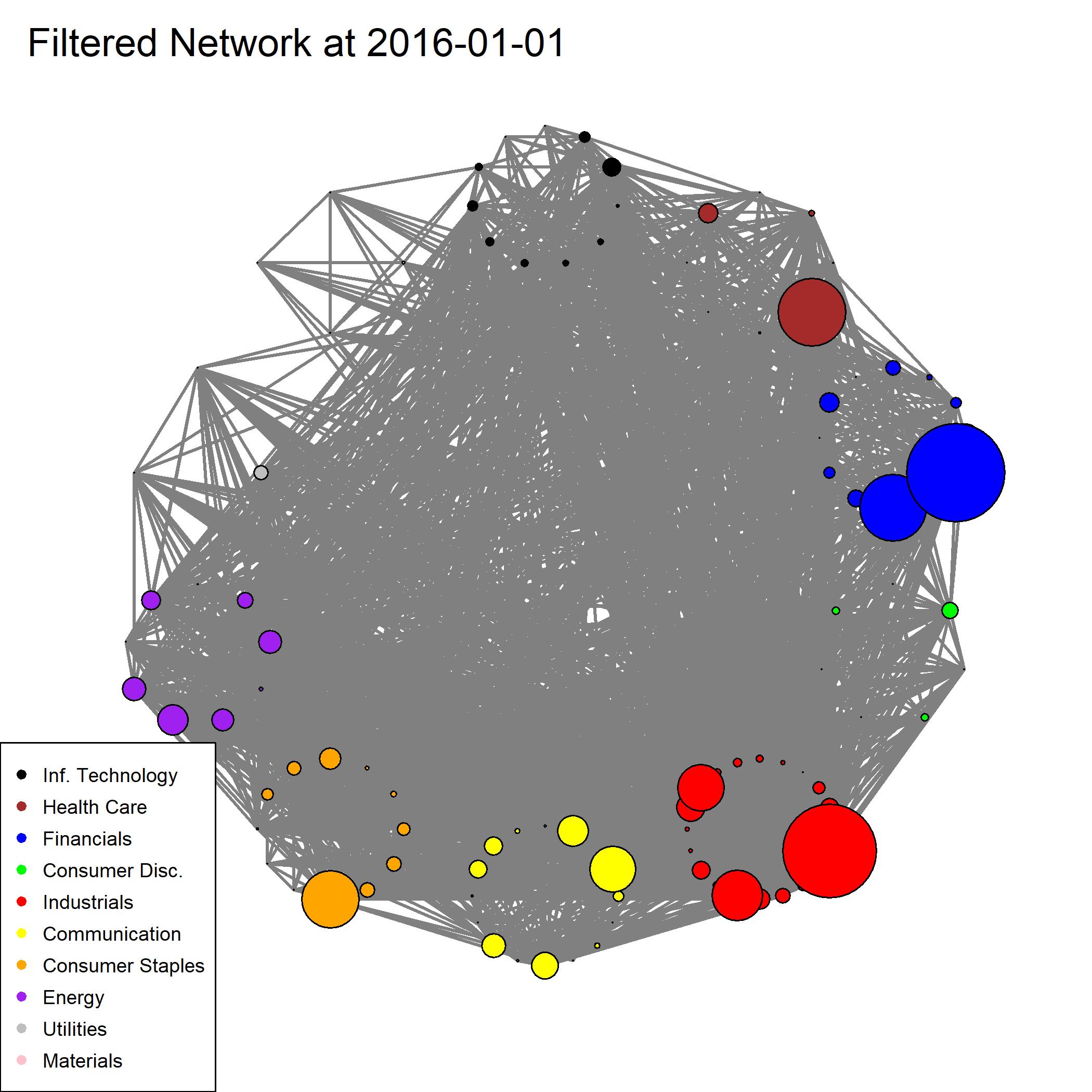
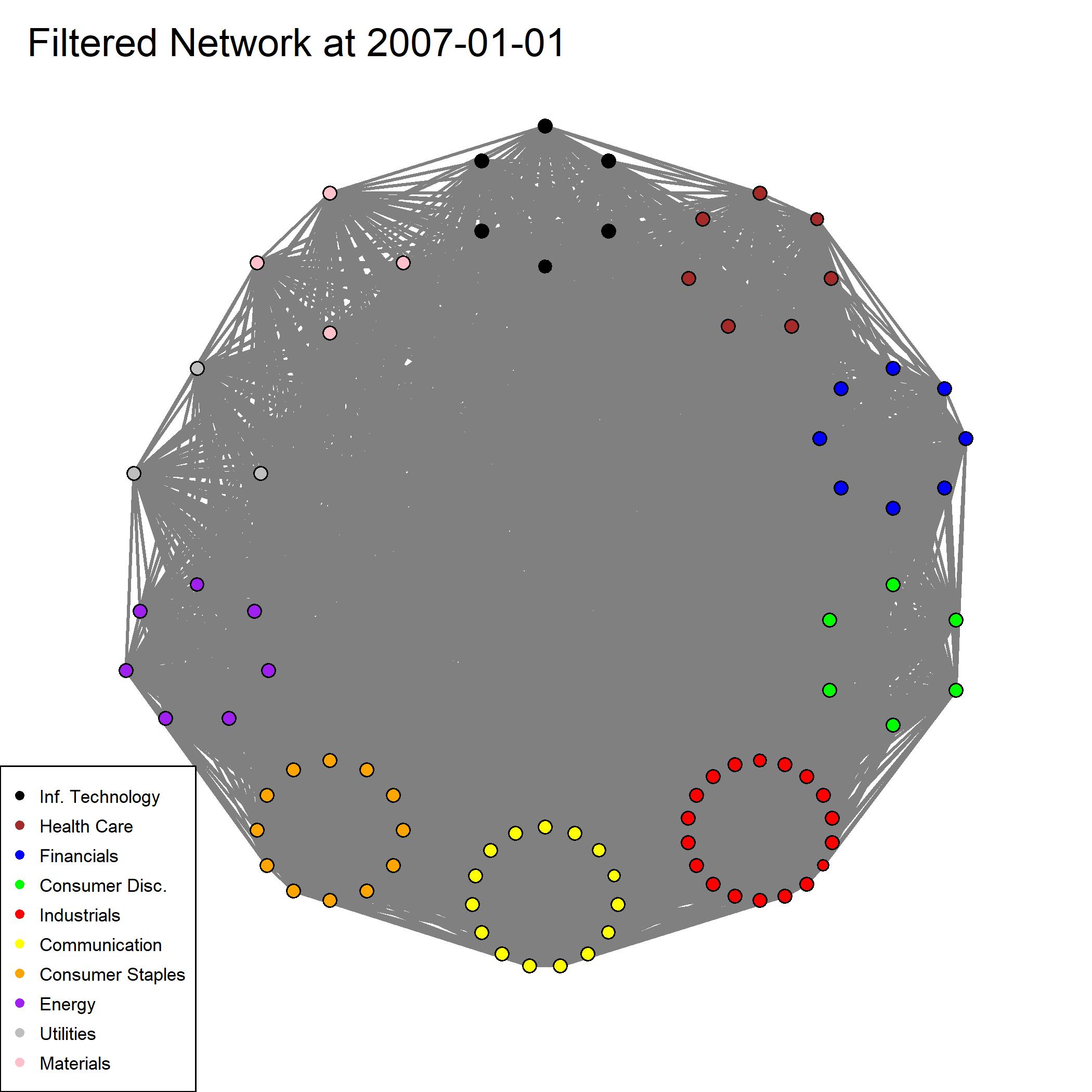
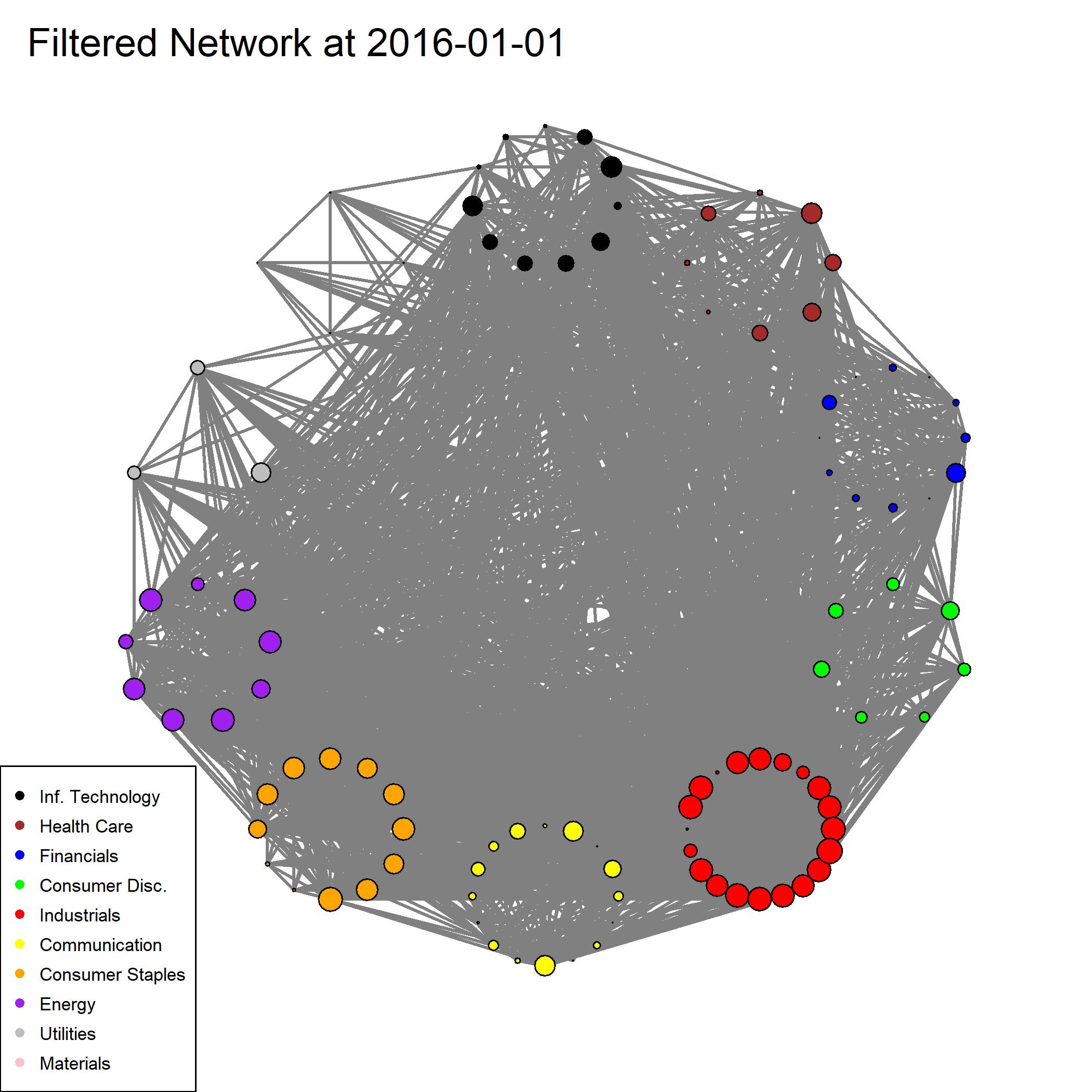
Figure 2: Filtered Networks at the end of 2006 and 2015. They refer to data of the two-year periods 2007-2008 and 2016-2017, respectively. Nodes are assets and edges’ weights are related to the correlation coefficients between returns of couple of assets (see Section 4.1 for details). Assets are grouped in 10 sectors, according to the financial classification reported in the legend. On the upper side, we focus on the role of relative betweenness centrality of each asset, namely, the bullets size is proportional to $b(i|G^{F}_{t})$. On the lower side, the bullets size is proportional to the relative eigenvector centrality.

This preliminary analysis suggests that it could be interesting to investigate not only the centrality of an asset with respect to both the financial market and the sector to which the asset belongs, but also the role/position of each sector in the whole network. According to formula (10), we computed both the average betweenness and the group betweenness centrality (see Figure 3). It is interesting to note that both indicators show a similar pattern over time, highlighting again differences between quiet and more turbulent periods. In both cases, we observe that, on average, the Financial, Industrial and Consumer Staples sectors are the most central. The Information Technology sector, that is actually the prominent sector of $S\&P$ 100 in terms of market capitalization, is increasing its centrality over time. It shows indeed a very low centrality with respect to other sectors at the beginning of the period and it has slowly increased his ranking over the last decade. On the other hand, the Energy subnetwork is extremely central in 2001, while it shows a very low centrality since 2012.

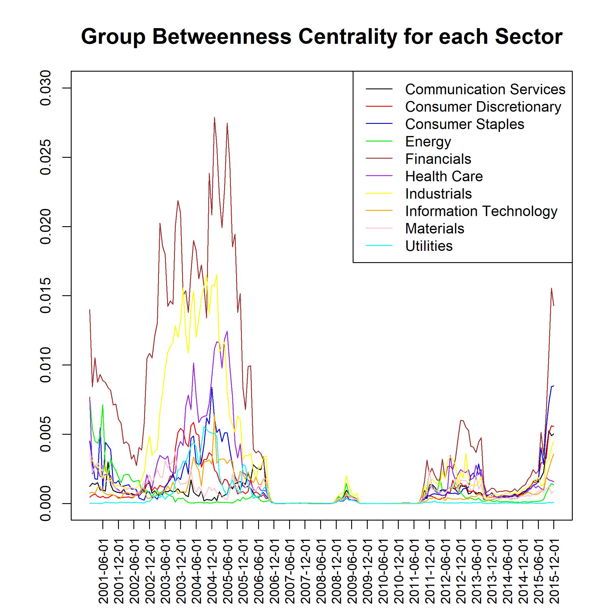
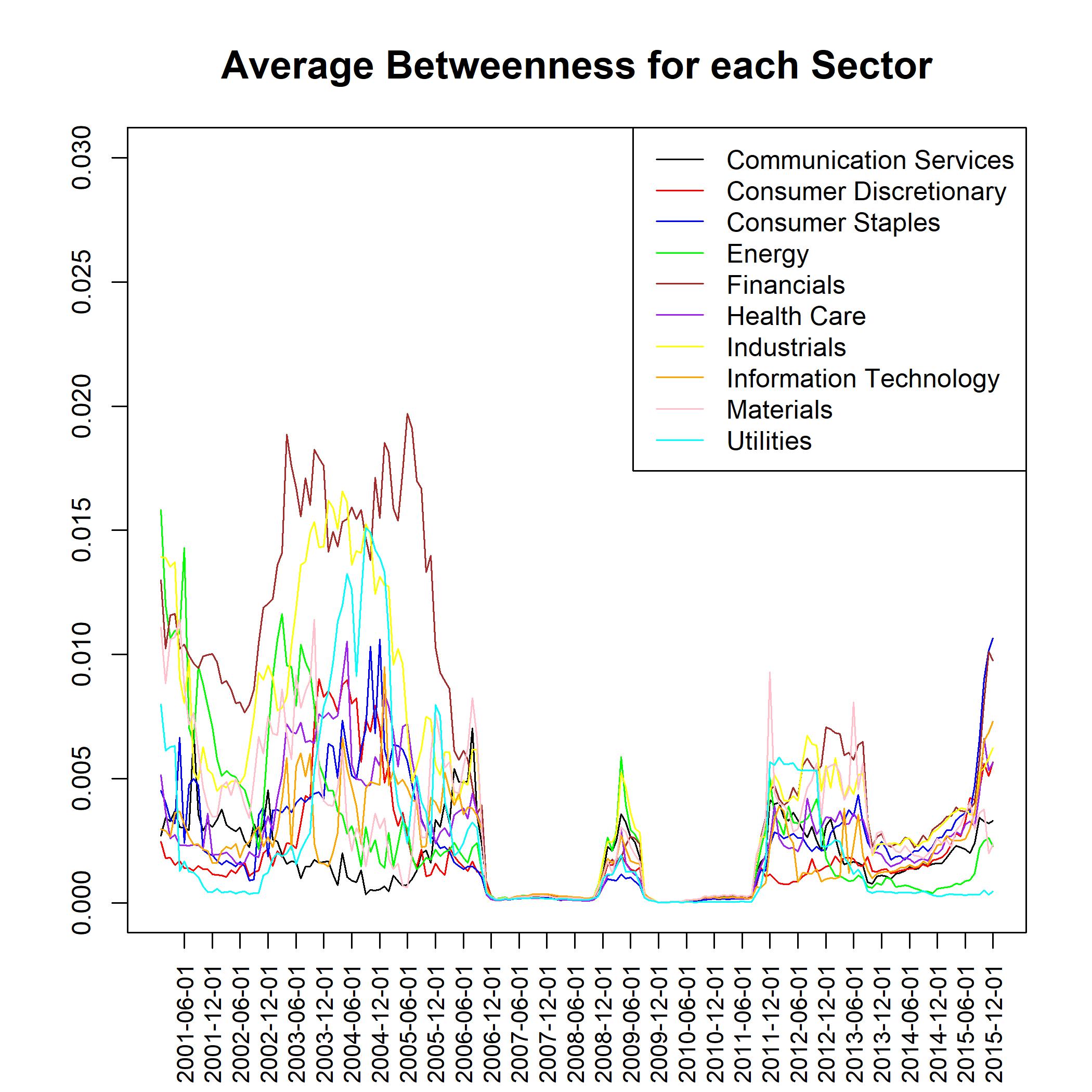
Figure 3: We display, on the left side, group betweenness centrality $b(G_{s})$ for each sector $s=1,...,10$ and for different time periods $t=1,...,181$. The average betweenness centrality $\bar{b}(G_{s})$ for each sector $s=1,...,10$ and for different time periods $t=1,...,181$ is instead reported on the right side.

Now, we focus on the behaviour of specific assets and we report in Tables 1 and 2 both the top and the bottom rankings in terms of relative betweenness centrality (computed by using formula (7)). The three ratios of the decomposition provided by formula (10) are also displayed. Values have been computed by considering the last period available (i.e. network “1-2016”). We observe that the most central assets do not necessarily belong to the most central sectors. On one hand, the financial sector is strongly represented by 6 assets in the top 15 ones. These assets are central in the network, but many of them are, at the same time, also relevant in their sector (as shown by the value of $b^{G}(i|G_{s})$). On the other hand, we can notice some examples of assets (like Home Depot and Amgen, for instance) that are really relevant in their sector, but belongs to a sector that, on average, is not very representative at the global level (as the $r^{b}_{G_{s}}$ coefficient shows for the Health Care and the Consumer Discretionary sectors).
It is also interesting to note that Amazon, that is one of the top ten constituents of the $S\&P$ 100 index, has a definitely low centrality in the network and it is also not extremely relevant in its sector.
Furthermore, we analyse in Table 3 how the top centrality assets are changed over time. To this end, we compare the top ranking in terms of relative betweenness in periods before and after the two crises, respectively. We observe how the composition drastically changed over time. At the beginning of the period (namely, the two-year 2001-2002), the financial and energy sectors almost make up completely the top group. The composition is a bit different in the subsequent periods, where assets of various sectors increase their central role. Interesting situation occurs immediately after the financial crisis, where industrial, costumer staples and health care appear as the prominent sectors, while the financial sector, except for some specific cases, significantly reduces his centrality. As noticed before, over the last period (namely the two-year 2016-2017), the financial sector becomes again prevalent.

Asset Name	Sector	$b(i|G)$	$b^{G}(i|G_{s})$	$k^{b}_{G_{s}}$	$r^{b}_{G_{s}}$
Mondelez	Consumer Staples	7.04	5.37	0.80	1.65
Berkshire Hathaway	Financials	6.71	3.05	1.46	1.51
Home Depot	Consumer Discretionary	4.84	5.63	0.98	0.88
PepsiCo Inc	Consumer Staples	4.77	3.64	0.80	1.65
Honeywell International	Industrials	4.12	5.93	0.72	0.96
Mastercard	Financials	3.63	1.65	1.46	1.51
Visa	Financials	3.34	1.51	1.46	1.51
Amgen	Health Care	3.29	13.45	0.28	0.87
Blackrock	Financials	2.82	1.28	1.46	1.51
Abbott Laboratories	Health Care	2.21	9.06	0.28	0.87
Microsoft Corp	Information Technology	2.19	3.96	0.49	1.13
Coca-Cola Company	Consumer Staples	2.04	1.56	0.80	1.65
U.S. Bancorp	Financials	2.04	0.93	1.46	1.51
Danaher Corp	Health Care	1.91	7.81	0.28	0.87
Johnson & Johnson	Health Care	1.76	7.19	0.28	0.87

Table 1: Top 15 ranking in terms of relative betweenness based on the network “1-2016”

Asset Name	Sector	$b(i|G)$	$b^{G}(i|G_{s})$	$k^{b}_{G_{s}}$	$r^{b}_{G_{s}}$
Amazon.com	Consumer Discretionary	0.025	0.029	0.982	0.875
ConocoPhillips	Energy	0.022	0.104	0.593	0.353
Raytheon Company	Industrials	0.021	0.030	0.721	0.964
Occidental Petroleum	Energy	0.019	0.090	0.593	0.353
American Express Company	Financials	0.018	0.008	1.464	1.505
Duke Energy	Utilities	0.017	1.186	0.194	0.072
Charter Communications	Communication Services	0.015	0.019	1.521	0.510
Nike	Consumer Discretionary	0.014	0.017	0.982	0.875
Monsanto	Materials	0.012	0.091	0.372	0.366
Lockheed Martin	Industrials	0.012	0.017	0.721	0.964
Southern Company	Utilities	0.009	0.644	0.194	0.072
Bristol-Myers Squibb Company	Health Care	0.006	0.024	0.280	0.872
Time Warner	Communication Services	0.006	0.007	1.521	0.510
CVS Health Corp	Health Care	0.002	0.008	0.280	0.872
Allergan Plc	Health Care	0.000	0.000	0.280	0.872

Table 2: Bottom 15 ranking in terms of relative betweenness based on the network “1-2016”

2001-2002			2004-2005			2013-2014			2016-2017
Asset	Sector	$b(i|G)$	Asset	Sector	$b(i|G)$	Asset	Sector	$b(i|G)$	Asset	Sector	$b(i|G)$
American Express	FI	7.11	Danaher	HC	8.24	Berkshire Hathaway	FI	3.55	Mondelez	CS	7.04
Citigroup	FI	7.03	JP Morgan	FI	7.34	Johnson & Johnson	HC	3.36	Berkshire Hathaway	FI	6.71
Morgan Stanley	FI	4.45	General Electric	IN	6.79	3M	MA	2.43	Home Depot	CD	4.84
Exxon Mobil	EN	4.27	Coca-Cola	CS	6.74	CVS	HC	2.23	PepsiCo	CS	4.77
Goldman Sachs	FI	3.55	Goldman Sachs	FI	5.01	Colgate-Palmolive	CS	2.22	Honeywell	IN	4.12
United Technologies	IN	3.21	Emerson Electric	IN	4.22	Mondelez	CS	2,18	Mastercard	FI	3.63
Bank of New York	FI	3.14	Home Depot	CD	3.90	Honeywell	IN	1.85	Visa	FI	3.34
JP Morgan	FI	2.95	Southern Company	UT	3.75	Danaher	HC	1.85	Amgen	HC	3.29
Wells Fargo	FI	2.94	Bank of America	FI	3,74	General Dynamics	IN	1.85	Blackrock	FI	2.82
Chevron	EN	2.55	Qualcomm	IT	2.86	Wells Fargo	FI	1.85	Abbott Laboratories	HC	2.21
General Electric	IN	2.20	Wells Fargo	FI	2.70	PepsiCo	CS	1.80	Microsoft	IT	2.19
Walt Disney	CO	2.14	Caterpillar	IN	2.49	Merck	HC	1.75	Coca-Cola	CS	2.04
U.S. Bancorp	FI	1.98	Bank of New York	FI	2.40	Philip Morris	CS	1.74	U.S. Bancorp	FI	2.04
Bank of America	FI	1.78	Morgan Stanley	FI	2.30	United Technologies	IN	1.72	Danaher Corp	HC	1.91
American International Group	FI	1.78	United Technologies	IN	2.09	Union Pacific	IN	1.71	Johnson & Johnson	HC	1.76

Table 3: Top 15 ranking in terms of relative betweenness at different time periods. Sectors have been denoted as follows: CO - Communication Services, CD - Consumer Discretionary, CS - Consumer Staples, EN- Energy, FI - Financial, HC - Health Care, IN- Industrials, IT - Information Technology, MA - Materials, UT - Utilities

Moving to the eigenvector centrality, Figure 4 reports both the average eigenvector and the group eigenvector centrality, according to formula (14). Unlike the betweenness measure, the average centrality of sectors seems to be more reactive than the group centrality during the periods of crisis.
Since the eigenvector centrality quantifies the power of the group, it could be expected that this measure is particularly sensitive to a crisis of the system. Usually associated with a financial crisis, as for those of 2007-2008, contagion can be manifested as negative externalities diffused among the entities of the system. Actually, the eigenvector group centrality is computed by means of the reduced model, where all the nodes of the same sector collapse in a single one leading to smooth differences between assets. Therefore, all sectors overreact moving towards the maximum value of centrality during the crisis periods, with the exception of the utilities’ sector. A more remarkable behaviour is the one of the average centrality, where specific individual vertex centrality prevails on the sector, driving the trend. In particular, Financial, Industrial and Energy sectors seem to be more influenced than others, like Consumer Staples and Health Care.

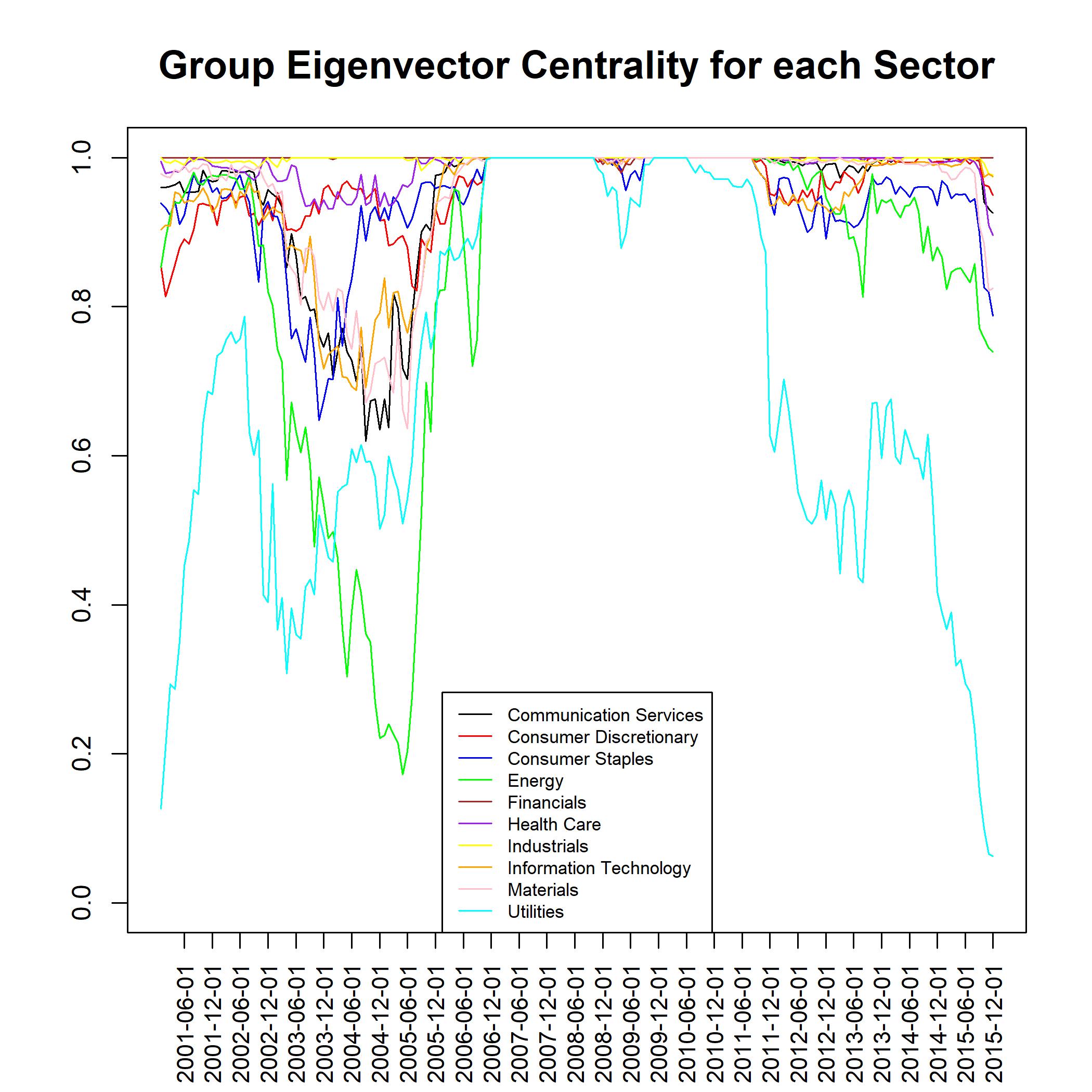
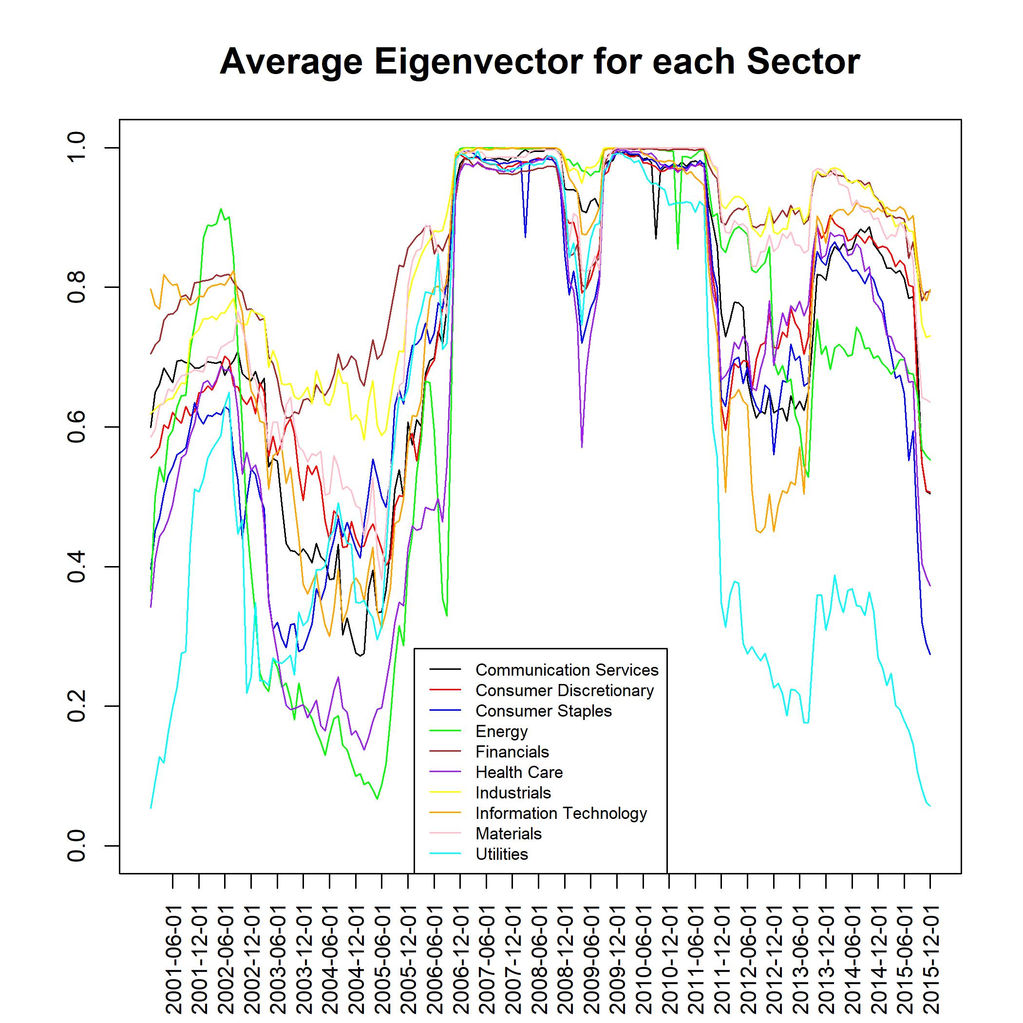
Figure 4: We display, on the left side, group eigenvector centrality $x(G_{s})$ for each sector $s=1,...,10$ and for different time periods $t=1,...,181$. On the right side, we report the average eigenvector centrality $\bar{x}(G_{s})$ for each sector $s=1,...,10$ and for different time periods $t=1,...,181$.

Now we focus on the individual relative eigenvector centrality, ranking the top and the bottom 15 (see Tables 4 and 5, respectively), referred to the last period available (i.e. the network “1-2016”). In particular, Table 4 reports the top 15 assets with highest relative eigenvector centrality in the period. The most part of the top ranked companies belongs to the financial sector. Financial companies appear as the most powerful one, both at individual level and as a part of a powerful group. Although such a sector has been significantly affected by the financial crisis, it has reinforced its position and dominates the international scene. Honeywell International is the only non-financial asset that belongs to the top 5 in terms of both betweenness and eigenvector centrality. This asset has been characterized during the period by a significant increase in the market value.
Table 5 lists, on the contrary, the 15 less central assets. The bottom of the ranking shows heterogeneity of the sectors: Utilities, Consumer Staples, Communication services and Health Care are among the less central sectors. The main difference with respect to relative betweenness (Table 2) is represented by the presence of several assets of Consumer Staples sector, probably reflecting a difficult period of the whole sector after the world crisis. In particular, the last two positions are occupied by Walmart and Target, that show a relative value significantly lower than all the other firms. At the end of 2015, Walmart saw its stock falling of 10%. In 2016, such a firm reported its first annual sales decline since 1980 and announced the closure of several stores. In 2017, Target Corporation shares suffered their biggest-ever price drop in active trade, as the discount retail giant struggles to cope with the “rapidly changing” behaviour of consumers. Target Corporation reported a profit that missed expectations and well below analyst projections.
Negative trends are also observed for other assets belonging to the 15 bottom ranked companies, for both eigenvector and betweenness centralities. For instance, the shares of the retail pharmacy giant CVS Health felt by more than 18% during 2016, according to data from S&P Global Market Intelligence. Bristol-Myers stock collapsed in 2017 after a disastrous cancer study failure. A combination of bad news and a general sell-off in the stock market is sending the Allergan stock down since 2016. What is most surprising with the drop is the rapidity of its decline with the market value almost halved in two years.
It is worth noting the case of Exelon and other assets of Utility sector. These assets are more central in the subgroup than in the whole market. Indeed, Exelon – which is one of the leader companies among the energy providers in the U.S. Utility sector – is instead not very central in the network; at the same time, its centrality is not so affected by the crisis, probably due to a lower dependence between this sector and the other ones.

Asset Name	Sector	$x(i|G)$	$x^{G}(i|G_{s})$	$k^{x}_{G_{s}}$	$r^{x}_{G_{s}}$
Berkshire Hathaway	Financials	1.800	1.000	1.260	1.428
Blackrock	Financials	1.751	0.973	1.260	1.428
Honeywell International	Industrials	1,723	0,980	1,338	1,314
U.S. Bancorp	Financials	1,719	0,955	1,260	1,428
JP Morgan	Financials	1,695	0,942	1,260	1,428
Citigroup	Financials	1,691	0,940	1,260	1,428
Visa	Financials	1,687	0,937	1,260	1,428
Mastercard	Financials	1,687	0,937	1,260	1,428
Bank of New York Mellon	Financials	1,684	0,936	1,260	1,428
Morgan Stanley	Financials	1,684	0,936	1,260	1,428
Intel	Information Technology	1,662	0,948	1,223	1,434
Goldman Sachs	Financials	1,659	0,922	1,260	1,428
Bank of America	Financials	1,650	0,917	1,260	1,428
Fedex	Industrials	1,640	0,932	1,338	1,314
Texas Instruments	Information Technology	1,623	0,925	1,223	1,434

Table 4: Top 15 ranking in terms of relative eigenvector based on the network “1-2016”

Asset Name	Sector	$x(i|G)$	$x^{G}(i|G_{s})$	$k^{x}_{G_{s}}$	$r^{x}_{G_{s}}$
Charter Communications	Communication Services	0.247	0.148	1.835	0.908
Verizon Communications	Communication Services	0.242	0.134	1.260	1.428
Eli Lilly and Company	Health Care	0.181	0.112	2.403	0.671
Simon Property Group	Financials	0.178	0.099	1.260	1.428
Altria Group	Consumer Staples	0.126	0.089	2.872	0.494
Exelon	Utilities	0.119	1.059	1.087	0.104
Allergan Plc	Health Care	0.112	0.070	2.403	0.671
Nextera Energy	Utilities	0.106	0.941	1.087	0.104
Duke Energy	Utilities	0.097	0.863	1.087	0.104
Costco Wholesale	Consumer Staples	0.093	0.066	2.872	0.494
Southern Company	Utilities	0.092	0.818	1.087	0.104
Bristol-Myers Squibb Company	Health Care	0.089	0.055	2.403	0.671
CVS Health	Health Care	0.088	0.054	2.403	0.671
Target	Consumer Staples	0.026	0.018	2.872	0.494
Walmart	Consumer Staples	0.014	0.010	2.872	0.494

Table 5: Bottom 15 ranking in terms of relative eigenvector based on the network “1-2016”

6 Conclusions and future research

The paper contains a new conceptualization of centrality measures which includes also the role of the single nodes and of the subgraphs of the network in the overall system. The scientific ground of the study lies in the need of exploring the relative relevance of such elements of a complex network in their real contextualization. The definition of relative centrality measures allows to compare nodes and subgraphs, also when they belong to different networks.

After a theoretical description of the model, some empirical experiments have been carried out. The employed dataset consists of the components of the $S\&P$ 100 index, which are assumed to be connected through their correlation coefficients. We focused on two measures (eigenvector and betweenness centrality) with extremely different characteristics, in order to discover the hidden role of influential firms in local groups. Results show that both measures provide additional insight than the simple degree centrality, that assures only a local view. From a general point of view, we detected an homogeneous behaviour of the relative centralities in all sectors during the period of crisis, in response to the increase of the assets correlation. The financial sector, that has suffered most, due to the effects of the crisis, has returned to have a powerful role and it prevails in conveying information. Industrial and Energy sectors also have increased their importance in terms of power and dominance. Centralities of assets and sectors not always go accordingly. Assets in some sectors, as Consumer Staple, Utilities and Communication, have diminished their importance, probably also reflecting how specific firms evolved over time. Results highlight the centrality of specific stocks (nodes) or sectors (subgraphs) in the overall system, and relevant insights have been derived under a purely economic point of view.
However, it is noteworthy that our proposal of decomposition of a relative centrality can be easily extended also to other relevant measures, as well as to oriented networks, in order to assess the emergence of opinion leaders at different levels for example in voting models. Moreover, the introduced methodological tools can be effectively applied to other relevant empirical data. An important example is the world trade network. In this specific case, relative and group centralities might be of interest for detecting the economic trading flows within the overall world context. In light of the possible applications of the presented centrality measures, we also point out the crucial role of such devices in describing the time-evolving properties of the networks topology. In this respect, we here deal with static measures on rolling time-windows, which can give insights on time-evolution when computed over different time periods. However, an extension to a dynamic setting can be of interest. To this aim, one should understand the dynamics underlying the evolution of relative and groups centrality measures by assessing the presence of regularities in the relationship between different time-realizations. Such an evolutionary rule would be reasonably of random nature, able to describe the future evolution of networks topology. This topic might contribute to effectively predict crucial economic and financial patterns, like the world trade and the financial stock markets.

Compliance with Ethical Standards:

Conflict of Interest: The authors declare that there is no conflict of interest.
Ethical approval: This article does not contain any studies with human participants or animals performed by any of the authors.

References

- Battiston et al (2010) Battiston S, Glattfelder JB, Garlaschelli D, Lillo F, Caldarelli G (2010) The structure of financial networks. In: Network Science, Springer, pp 131–163
- Beber et al (2011) Beber A, Brandt MW, Kavajecz KA (2011) What does equity sector orderflow tell us about the economy? The Review of Financial Studies 24(11):3688–3730
- Benzi (2015) Benzi M, Klymko C (2015) On the Limiting Behavior of Parameter-Dependent Network Centrality Measures, SIAM Journal on Matrix Analysis and Applications, 36: 686–706
- Bloomberg (2012) Bloomberg (2012) Bloomberg professional. [online]. Available at: Subscription Service (Accessed: 30 November 2012)
- Bonacich (1972) Bonacich P (1972) Factoring and weighting approaches to status scores and clique identification. Journal of mathematical sociology 2(1):113–120
- Bonacich (1987) Bonacich P (1987) Power and centrality: a family of measures. American Journal of Sociology 92:1170–1182
- Bonacich (1991) Bonacich P (1991) Simultaneous group and individual centralities. Social networks 13(2):155–168
- Borgatti et al. (2006) Borgatti S P, Carley K M, Krakhardt D (2006), On the Robustness of Centrality Measures Under Conditions of Imperfect Data, Social Networks 28(2): 124-136.
- Cerqueti et al (2018) Cerqueti R, Ferraro G, Iovanella A (2018), A new measure for community structures through indirect social connections. Expert Systems with Applications 114:196–209.
- Cinelli et al (2017) Cinelli M, Ferraro G, Iovanella A (2017a), Structural bounds on the dyadic effect. Journal of Complex Networks 5(5):694–711.
- Cinelli et al (2017) Cinelli M, Ferraro G, Iovanella A (2017b), Resilience of core-periphery networks in the case of rich-club. Complexity Article ID 6548362.
- Cinelli et al (2018) Cinelli M, Ferraro G, Iovanella A (2018) Rich-club ordering and the dyadic effect: Two interrelated phenomena. Physica A: Statistical Mechanics and its Applications 490:808–818
- Colizza et al (2006) Colizza V, Flammini A, Serrano MA, Vespignani A (2006) Detecting rich-club ordering in complex networks. Nature physics 2(2):110
- Estrada and Rodriguez-Velazquez (2005) Estrada E, Rodriguez-Velazquez JA (2005) Subgraph centrality in complex networks. Physical Review E 71(5):056,103
- Everett and Borgatti (1999) Everett MG, Borgatti SP (1999) The centrality of groups and classes. The Journal of mathematical sociology 23(3):181–201
- Freeman (1979) Freeman L (1979) Centrality in social networks - conceptual clarification. Social networks 1:215–239
- Freeman (1977) Freeman LC (1977) A set of measures of centrality based on betweenness. Sociometry 40(1):35–41
- Freeman and Freeman (1979) Freeman S, Freeman L (1979) The networkers network: a study of the impact of a new communications medium on sociometric structure. Social Science Research Reports 46 103:109–115
- Harary (1969) Harary F (1969) Graph theory. Addison-Wesley
- Katz (1953) Katz L (1953) A new status index derived from sociometric analysis. Psychometrika 18(1):39-43
- Landherr et al. (2010) Landherr A, Friedl B, Heidemann J (2010) A critical review of centrality measures in social networks, Business & Information Systems Engineering 2(6): 371–385
- Ma and Ma (2019) Ma Q, Ma J (2019) A robust method to discover influential users in social networks. Soft Computing 23:1283–1295
- Martin et al. (2014) Martin T, Zhang X, Newman, M E J (2014) Localization and centrality in networks, Physical Review E 90(5).
- Newman (2010) Newman M (2010) Networks: An introduction. Oxford University Press
- Opsahl et al (2008) Opsahl T, Colizza V, Panzarasa P, Ramasco J (2008) Prominence and control: the weighted rich-club effect. Physical Review Letters 110(18):189903
- Peralta and Zareei (2016) Peralta G, Zareei A (2016) A network approach to portfolio selection. Journal of Empirical Finance 38(A):157–180
- Perra and Fortunato (2008) Perra N, Fortunato S (2008) Spectral centrality measures in complex networks. Physical Review E 78(3):036,107
- Pozzi et al (2013) Pozzi F, Di Matteo T, Aste T (2013) Spread of risk across financial markets: better to invest in the peripheries. Scientific reports 3
- Wang et al (2011) Wang J, Mo H, Wang F, Jin F (2011) Exploring the network structure and nodal centrality of china’s air transport network: A complex network approach. Journal of Transport Geography 19(4):712–721
- Wasserman and Faust (1994) Wasserman S, Faust K (1994) Social Network Analysis: Methods and Applications. Cambridge University Press, New York, NY., 1607.00509
- Watts (2004) Watts DJ (2004) Small worlds: the dynamics of networks between order and randomness, vol 9. Princeton University Press