Non-linear spin torque, pumping and cooling in superconductor/ferromagnet systems

Abstract

We study the effects of the coupling between magnetization dynamics and the electronic degrees of freedom in a heterostructure of a metallic nanomagnet with dynamic magnetization coupled with a superconductor containing a steady spin-splitting field. We predict how this system exhibits a non-linear spin torque, which can be driven either with a temperature difference or a voltage across the interface. We generalize this notion to arbitrary magnetization precession by deriving a Keldysh action for the interface, describing the coupled charge, heat and spin transport in the presence of a precessing magnetization. We characterize the effect of superconductivity on the precession damping and the anti-damping torques. We also predict the full non-linear characteristic of the Onsager counterparts of the torque, showing up via pumped charge and heat currents. For the latter, we predict a spin-pumping cooling effect, where the magnetization dynamics can cool either the nanomagnet or the superconductor.

I Introduction

The intriguing possibility to control magnetization dynamics by spin torque suggested over two decades ago Slonczewski (1996) and its reciprocal counterpart Johnson and Silsbee (1987); Bauer et al. (2012) of spin pumping Tserkovnyak et al. (2002) have been widely studied in magnetic systems. In such systems charge and spin transport are closely linked and need to be treated on the same footing. Recently there has also been increased interest in coupling superconductors to magnets and finding out how superconductivity affects the magnetization dynamics Bell et al. (2008); Houzet (2008); Jeon et al. (2018); Yao et al. (2018); Jeon et al. (2019); Rogdakis et al. (2019); Morten et al. (2008); Skadsem et al. (2011); Inoue et al. (2017); Teber et al. (2010); Richard et al. (2012); Holmqvist et al. (2014); Hammar and Fransson (2017); Kato et al. (2019); Dutta et al. (2017). On the other hand, recent work has shown that a combination of magnetic and superconducting systems results in giant thermoelectric effects Machon et al. (2013); Ozaeta et al. (2014); Silaev et al. (2015); Bergeret et al. (2018); Heikkilä et al. (2019) which couple charge and heat currents. These works Ozaeta et al. (2014); Silaev et al. (2015) also imply a coupling of spin and heat. However, a general description of the implications for the magnetization dynamics, dynamical heat pumping effects, and the behavior in the non-linear regime at energies comparable to the superconductor gap $\Delta$, has been lacking.

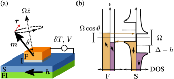
Figure 1: (a) Schematic ferromagnetic island–superconductor tunnel junction (F/I/S) setup. The direction $\bm{m}$ of magnetization in F precesses at a rate $\Omega$ at an angle $\theta$ around the axis ($\hat{z}$) of its effective field. Electron tunneling and intrinsic damping produces torque $\bm{\tau}$ on $\bm{m}$. The superconductor has an internal spin splitting exchange field $\bm{h}$, from external magnetic field, or a ferromagnetic insulator (FI) bilayer structure Tedrow et al. (1986). We consider also thermal and electric biasing $(\delta T,V)$. (b) “Semiconductor picture” for pumping, in the frame rotating with $\bm{m}$ (for $\bm{h}\parallel\hat{z}$). Grey solid line is the chemical potential when $\Omega=0$. Increasing the precession frequency to $\Omega\neq 0$ shifts both the spectrum and the chemical potentials (dashed lines) by $\Omega\cos\theta$ in F and by $\Omega$ in S. The exchange field $\bm{h}$ only shifts the spectrum in S.

In this work, we fill this gap by constructing a theory which provides a combined description of pumped charge and heat currents, spin torques, magnetization damping, voltage and thermal bias. We consider a metallic nanomagnet F with a magnetization precessing at a rate $\Omega$ which is determined by an external magnetic field, the shape of the magnet and the crystal anisotropy, Kittel (1948) at a slowly varying angle $\theta$ to the precession axis [Fig. 1(a)]. The magnet is tunnel coupled to a superconducting electrode S that also contains a constant spin-splitting (exchange or Zeeman) field Tedrow et al. (1986); Tokuyasu et al. (1988).

Main features of the problem can be understood in a tunneling model, shown schematically in Fig. 1(b). Both the spin splitting $h$ and nonzero $\Omega$ shift the spectrum, whereas $\Omega$ generates also effective spin-dependent chemical potential shifts Tserkovnyak et al. (2005) providing a driving force which pumps the currents across the interface. The interplay of the two enables a coupling between the magnetization dynamics and the linear-response thermoelectric effect Machon et al. (2013); Ozaeta et al. (2014); Bergeret et al. (2018) originating from the spin-selective breaking of the electron-hole symmetry in the superconductor with respect to the chemical potential. As a consequence, a temperature difference between the two systems leads to a thermal spin torque, which in a suitable parameter regime yields an anti-damping sufficient to obtain flipping or stable precession of the nanomagnet. The Onsager counterpart of the thermal spin torque is a Peltier-type cooling (or heating) driven by the precessing magnetization. In the non-linear response, the precession also pumps a charge current, as already shown in Trif and Tserkovnyak (2013). We discuss the general picture for the spin-split superconductor, and, in addition to the thermomagnetic effects, find the Keldysh action [Eq. (20)] describing the stochastic properties of the S/F junction. The action allows identifying thermodynamical constraints, current noises, a spintronic fluctuation theorem and describes the probability distribution of the magnetization direction and the spectrum of its oscillations.

The manuscript is structured as follows: We introduce a simple tunneling model in Sec. II and discuss the tunneling currents in Sec. III. Implications on magnetization dynamics are considered in Sec. IV, including thermal transport associated with the ferromagnetic resonance and physics of spin torque oscillators driven by the thermal effects. In Sec. V we focus on studying the stochastic magnetization dynamics based on a Keldysh action approach to the tunneling model, and discuss probability distributions and linewidths for the oscillators. We conclude in Sec. VI. Certain details of derivations are postponed to the Appendixes.

II Tunneling model

The main effects can be understood with a tunneling Hamiltonian description (below $\hbar=e=k_{B}=1$),

$$H=H_{S}+\hat{R}(t)H_{F}\hat{R}(t)^{\dagger}+\sum_{jj^{\prime}\sigma}W_{jj^{\prime}}e^{-iVt}c^{\dagger}_{j\sigma}d_{j^{\prime}\sigma}+\mathrm{h.c.}\,,$$ (1)

where $c_{j\sigma}$ and $d_{j\sigma}$ are the F and S conduction electron operators and $W$ the tunneling matrix elements for spin/momentum states $\sigma=\pm$, $\bm{p}_{j}$, and $V$ is a bias voltage. The Hamiltonian $H_{S}$ describes the spin-split superconductor Bergeret et al. (2018), and $H_{F}$ the magnet with magnetization parallel to the $\hat{z}$-direction. The magnetization direction $\bm{m}(t)=(\cos\phi\sin\theta,\sin\phi\sin\theta,\cos\theta)$ is specified by a spin rotation matrix $\hat{R}(t)c_{j\sigma}\hat{R}(t)^{\dagger}=\sum_{\sigma^{\prime}}R_{\sigma\sigma^{\prime}}(t)c_{j\sigma^{\prime}}$. In the frame rotating with $R$ Tserkovnyak et al. (2005, 2008), assuming $\bm{m}(t)$ varies adiabatically so that an equilibrium electron distribution is maintained, the Berry phase $\varphi(t)=\int^{t}\mathrm{d}t^{\prime}\,\dot{\phi}(1-\cos\theta)$ can be absorbed (c.f. Refs. Flebus et al., 2017, Shnirman et al., 2015 and Appendix B) to the spin rotation

$$R=e^{-i\phi(t)\sigma_{z}/2}e^{-i\theta(t)\sigma_{y}/2}e^{i\phi(t)\sigma_{z}/2}e^{-i\varphi(t)\sigma_{z}/2}\,,$$ (2)

where $\sigma_{x/y/z}$ are the spin matrices. Varying $\bm{m}(t)$ results to effective spin-dependent voltages Tserkovnyak et al. (2008) in the tunneling part. For uniform precession, they are $\Omega_{\sigma\sigma^{\prime}}=(\sigma-\sigma^{\prime}\cos\theta)\Omega/2$ (see Fig. 1b). From the model, we can compute in leading order in $W$ the tunneling charge, energy, and spin currents ($I_{c}$, $\dot{E}$, $\bm{I}_{s}$) via a standard Green function approach (see Ref. Bergeret et al., 2012 and Appendix A). The assumption of local equilibrium implies that the rates of tunneling and other nonequilibrium-generating processes on the magnetic island should be small compared to electron relaxation. Ludwig et al. (2017, 2019a, 2019b)

Consider precession with frequency $\Omega$ around the $z$-axis, $\phi(t)=\Omega{}t$ with $|\dot{\theta}|\ll\Omega$. From the above model, we find the time-averaged currents and $\hbar\overline{\tau_{z}}=-\overline{(\bm{m}\times{}\bm{I}_{s}\times\bm{m})_{z}}$, Slonczewski (1996); Tserkovnyak et al. (2005) the $z$-component of the time-averaged spin transfer torque:

$$\overline{I_{c}} =\frac{G_{T}}{2e}\int_{-\infty}^{\infty}\mathrm{d}\epsilon\,\sum_{\sigma\sigma^{\prime}}\langle{\sigma}|{}\sigma^{\prime}\rangle^{2}N_{S,\sigma}N_{F,\sigma^{\prime}}[f_{F}-f_{S}]\,,$$ (3)

$$\overline{\dot{E}_{S}} =\frac{G_{T}}{2e^{2}}\int_{-\infty}^{\infty}\mathrm{d}\epsilon\,\sum_{\sigma\sigma^{\prime}}\epsilon\langle{\sigma}|{}\sigma^{\prime}\rangle^{2}N_{S,\sigma}N_{F,\sigma^{\prime}}[f_{F}-f_{S}]\,,$$ (4)

$$\overline{\tau_{z}} =-\frac{G_{T}\sin^{2}\theta}{8e^{2}}\int_{-\infty}^{\infty}\mathrm{d}\epsilon\,\!\sum_{\sigma\sigma^{\prime}}\sigma N_{S,\sigma}N_{F,\sigma^{\prime}}[f_{F}-f_{S}]\,.$$ (5)

Here, $f_{F}=f_{0}(\epsilon-V-\Omega_{\sigma\sigma^{\prime}},T_{F})$, $f_{S}=f_{0}(\epsilon,T_{S})$ are the Fermi distribution functions in F and S, $\langle{\sigma}|{}\sigma^{\prime}\rangle^{2}=(1+\sigma\sigma^{\prime}\cos\theta)/2$ the spin overlap between $\bm{m}$ and the $z$-axis, and $N_{S/F,\sigma=\pm}$ the densities of states (DOS) for up/down spins (quantization axis $\bm{m}(t)$ for F, and $\hat{z}$ for S) normalized by the Fermi level DOS per spin, and $G_{T}$ the tunneling conductance. Of these, Eq. (3) was previously discussed in Ref. Trif and Tserkovnyak, 2013 for $\bm{h}=0$. Using a basic model for F and S, we have $N_{F,\sigma}=1+\sigma{}P$ and $N_{S,\sigma}=\sum_{\pm}\frac{1\pm{}\sigma\hat{h}\cdot\hat{z}}{2}N_{0}(\epsilon\mp{}h)$, where $P=(\nu_{F,+}-\nu_{F,-})/(\nu_{F,+}+\nu_{F,-})$ is the spin polarization in terms of the majority/minority Fermi level DOS $\nu_{F,\pm}$, and $N_{0}(\epsilon)$ the Bardeen-Cooper-Schrieffer density of states Tinkham (2004). The tunneling described by Eqs. (3–5) can be understood in a semiconductor picture, as shown in Fig. 1b. The broken electron-hole symmetry around the chemical potentials for both spins in S and spin polarization in F results to thermally driven spin currents causing torques, and the rotation-induced potential shifts pump charge and heat currents.

III Tunneling currents

Expanding for small voltage bias $V$, temperature difference $\delta T=T_{S}-T_{F}$, and the precession speed $\Omega$, the time-averaged currents are described by a linear-response matrix:

$$\begin{pmatrix}\overline{I_{c}}\\ \overline{\dot{E}_{S}}\\ \overline{\tau_{z}}\end{pmatrix}=\begin{pmatrix}G&P\alpha\cos\theta&0\\ P\alpha\cos\theta&G_{\rm th}T&\frac{\alpha}{2}\sin^{2}\theta\\ 0&-\frac{\alpha}{2}\sin^{2}\theta&-\frac{G}{4}\sin^{2}\theta\end{pmatrix}\begin{pmatrix}V\\ -\delta T/T\\ \Omega\end{pmatrix}\,,$$ (6)

where $G$ and $G_{\rm th}$ are the linear-response electrical and thermal conductances. Here, $\alpha=-(G_{T}/2)\int_{-\infty}^{\infty}\mathrm{d}\epsilon\,\epsilon{}[N_{S,+}(\epsilon)-N_{S,-}(\epsilon)]f_{0}^{\prime}(\epsilon)$ is a thermoelectric coefficient, Machon et al. (2013); Ozaeta et al. (2014) which originates from the exchange field $h$ generating the electron-hole asymmetry in the superconductor. It is nonzero only when S is both superconducting and has a spin splitting $h\neq 0$. The response matrix $L$ in Eq. (6) has the Onsager symmetry $L_{ij}=L_{ji}^{\rm tr}$, where tr refers to time-reversal, $\alpha^{\rm tr}=-\alpha$, $P^{\rm tr}=-P$.

The coefficient for charge pumping is here zero, unlike in the ferromagnet–ferromagnet case, Tserkovnyak et al. (2008) because the spin-(anti)symmetrized DOS of S is also (anti)symmetric in energy. This also suppresses linear-response contributions to charge current from thermal magnetization fluctuations, Flebus et al. (2017) which are also related to the magnon spin–Seebeck effect Bauer et al. (2012); Flebus et al. (2017); Kato et al. (2019).

Importantly, the spin splitting of the superconductor enables the precession to pump energy current at linear response, and as its Onsager counterpart, there is nonzero thermal spin torque (terms with $\alpha\neq 0$). This is made possible by the nonzero thermoelectric coefficient Machon et al. (2013); Ozaeta et al. (2014) driving spin currents due to a temperature difference. This effect is (in metals) parametrically larger by a factor $\varepsilon_{F}/\Delta\gg 1$ than that from normal-state DOS asymmetry Hatami et al. (2007); Bauer et al. (2012); Ludwig et al. (2019a) in systems with Fermi energy $\varepsilon_{F}$.

III.1 Symmetries

Let us now consider the joint probability $P$ of changes $\delta{}n_{s}$ and $\delta{}E_{S}$ in the electron number and energy of S, and a change $\delta{}m_{z}$ in the magnetization of F, during a time interval of length $t_{0}$. It satisfies a fluctuation relation Virtanen and Heikkilä (2017); Utsumi and Taniguchi (2015):

$$P_{t_{0}}(\delta{}n,\delta{}E_{S},\delta{}m_{z}) =e^{T_{F}^{-1}V\delta n+(T_{S}^{-1}-T_{F}^{-1})\delta E_{S}+T_{F}^{-1}\Omega\mathcal{S}\delta{}m_{z}}$$

$$\quad\times P_{t_{0}}^{\rm tr}(-\delta{}n,-\delta{}E_{S},\delta{}m_{z})\,.$$ (7)

Here, we denote $\mathcal{S}={\cal V}M_{s}/(\hbar\gamma)$ as the effective macrospin of the ferromagnetic island, $\mathcal{V}$ and $\gamma$ are the F volume and gyromagnetic ratio and $M_{s}$ the magnetization. Moreover, $P^{\rm tr}$ corresponds to reversed polarizations and precession ($N_{S/F,\sigma}\mapsto{}N_{S/F,-\sigma}$, $\Omega\mapsto-\Omega$). The Onsager symmetry of $L_{ij}$ in Eq. (6) is a consequence of fluctuation relations Andrieux and Gaspard (2004). The energy transfer $\delta{}E_{F}$ into the ferromagnet (generally, $\delta{}E_{F}\neq\delta{}E_{S}$) is determined by energy conservation $\delta{}E_{F}+\delta{}E_{S}=V\delta{}n+\Omega\mathcal{S}\delta{}m_{z}$, which implies $\overline{\dot{E}_{S}+\dot{E}_{F}}=\overline{I_{c}}V-\Omega\overline{\tau_{z}}$. These results arise from the symmetries of Eqs. (19, 20) below, for the case where there is no external magnetic drive.

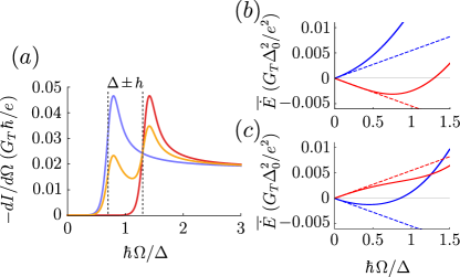
Figure 2: (a) Pumped differential current for $T_{S}=T_{F}=0.1\,T_{C}$ where $T_{C}$ is the critical temperature of the superconductor. Blue, yellow and red lines are for $\bm{h}=-h\hat{z},h\hat{x},h\hat{z}$, respectively. (b) and (c) Energy current into the superconductor $\overline{\dot{E}_{S}}$ (blue line) and into the magnet $\overline{\dot{E}_{F}}$ (red line) for (b) $\bm{h}=-h\hat{z}$ and for (c) $\bm{h}=h\hat{z}$. F and S are at temperature $T=0.6\,T_{C}$. Dashed lines represent the linear response. In all figures, $V=0$, $\theta=\frac{\pi}{8}$, $P=1$ and $h=0.3\Delta_{0}$, where $\Delta_{0}$ is the superconductor gap at zero temperature.

III.2 Non-linear response

The pumped charge current is shown in Fig. 2(a), and the energy current into S in Fig. 2(b). The charge pumping is nonzero above the quasiparticle gap, $|\Omega|\gtrsim\Delta\pm{}h$. Trif and Tserkovnyak (2013) The heat current shows the presence of a region of cooling of either of the two leads, depending on the relative orientation of $\bm{h}$ and $\Omega\hat{z}$. Nonzero $h$ enables the N/S cooling effect to be present already at linear response, similarly as with voltage bias Bergeret et al. (2018); Giazotto et al. (2006).

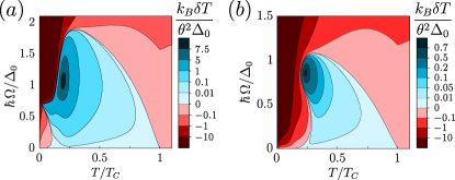
Figure 3: Electromagnetically driven FMR induced refrigeration for $\bm{h}=-0.3\Delta_{0}\hat{z}$, $P=1$, and $A_{0}=0.1\hbar G_{T}/(e^{2}\mathcal{S})$. (a) For $\lambda=0$, and (b) for $\lambda=1$. Dynes broadening $\Gamma=10^{-3}\Delta_{0}$ was assumed Dynes et al. (1984).

IV Magnetization dynamics

The Landau–Lifshitz–Gilbert–Slonczewski (LLG) equation for the tilt angle is

$$-\mathcal{S}\partial_{t}\cos\theta=\overline{\tau_{z}}-\mathcal{S}A_{0}\Omega\sin^{2}\theta+\eta\,,$$ (8)

where the spin transfer torque $\overline{\tau_{z}}$ is given by Eq. (5). We include the intrinsic Gilbert damping Tserkovnyak et al. (2005) phenomenologically, and $A_{0}$ is the dimensionless damping constant. Moreover, $\eta$ is a Langevin term describing the torque noise Chudnovskiy et al. (2008); Basko and Vavilov (2009); Shnirman et al. (2015); Virtanen and Heikkilä (2017) with the correlation function $\langle{\eta(t)\eta(t^{\prime})}\rangle=2[D(\theta)+\mathcal{S}A_{0}T]\sin^{2}(\theta)\delta(t-t^{\prime})$; see below. Equilibrium torques are here included in the LLG effective magnetic field $\Omega\hat{z}$ (see Appendix A). We consider the limit of weak damping, where it is sufficient to consider only the equation for the $z$-component.

IV.1 Heat balance in ferromagnetic resonance

Let us consider a ferromagnetic resonance (FMR) Kittel (1948) in a thin magnetic layer on a spin-split S, driven by a resonant circularly polarized rf magnetic field (at frequency $\omega=\Omega$), and in the case of S acting as a reservoir at a fixed temperature $T$. The electrical circuit is open, so that no charge flows between F and S. The FMR driving acts as a power source. We assume that a fraction $\lambda\in[0,1]$ of the power dissipated by the intrinsic Gilbert damping heats the F electrons; the value of $\lambda$ depends on into which bath(s) its microscopic mechanism dissipates the energy (see also Sec. V.1 below). In a steady state, the total energy current into F, the overall torque, and the charge current are zero:

$$\overline{\dot{E}_{F,\rm tot}}=\overline{\dot{E}_{F}}+\lambda\overline{P_{G}} =0,$$ (9)

$$\overline{\tau_{z}}+\overline{\tau_{z,\rm rf}}+\overline{\tau_{z,G}} =0,$$ (10)

$$\overline{I_{c}} =0,$$ (11)

where $\overline{\tau_{z}}$ and $\overline{I_{c}}$ are the contributions related to the tunneling between F and S, from Eqs. (3,5), and $\overline{\dot{E}_{F}}=\overline{I}_{c}V-\Omega\overline{\tau}_{z}-\overline{\dot{E}_{S}}$ is found from the tunneling model via a similar calculation as in Eq. (4). Moreover, $\overline{\tau_{z,G}}=-\mathcal{S}A_{0}\Omega\sin^{2}(\theta)$ and $\overline{P_{G}}=\mathcal{S}A_{0}\Omega^{2}\sin^{2}(\theta)$ are the torque due to the intrinsic damping and the rate of work done by it. At resonance, the rf drive creates a torque $\overline{\tau_{z,\rm rf}}=\gamma\mathcal{S}(\bm{m}\times\bm{h}_{\rm rf})_{z}=\gamma\mathcal{S}h_{\rm rf}\sin\theta$, where $h_{\rm rf}$ is the amplitude of the rf field. From the above it follows that the power

$$\overline{\dot{E}_{S}}+\overline{\dot{E}_{F,\rm tot}}=\overline{P_{\rm rf}}-(1-\lambda)\overline{P_{G}}$$ (12)

is absorbed by the electron system, where $\overline{P_{\rm rf}}=\Omega\overline{\tau_{z,\rm rf}}$ is the total rf power absorbed at resonance Tserkovnyak et al. (2005).

Expanding Eqs. (3–5) in the linear order in $V$, $\delta T/T$ and $\theta^{2}$, but not in $\Omega$, we find the charge and heat currents

$$\begin{pmatrix}\overline{I_{c}}\\ \overline{\dot{E}_{S}}\\ \overline{\tau_{z}}\end{pmatrix}=\begin{pmatrix}G&P\alpha&P(G-\widetilde{G})\\ P\alpha&G_{\rm th}T&\alpha+\widetilde{\alpha}+\frac{\widetilde{G}\Omega}{2}\\ 0&0&-\widetilde{G}\end{pmatrix}\begin{pmatrix}V\\ -\delta T/T\\ \frac{\Omega}{4}\theta^{2}\end{pmatrix}.$$ (13)

Unlike the linear-response matrix in Eq. (6), the above matrix is not symmetric, as there is no Onsager reciprocity between $\overline{\tau_{z}}$ and $\theta^{2}$. The coefficients are

$$\widetilde{\alpha} =\frac{G_{T}}{2}\int_{-\infty}^{\infty}\mkern-10.0mu\mathrm{d}\epsilon\,\sum_{\sigma}\left(\epsilon-\frac{\sigma\Omega}{2}\right)N_{S,\sigma}(\epsilon)\frac{f_{0}(\epsilon{-}\sigma\Omega)-f_{0}(\epsilon)}{\Omega}$$ (14)

$$\widetilde{G} =\frac{G_{T}}{2}\int_{-\infty}^{\infty}\mathrm{d}\epsilon\,\sum_{\sigma}\sigma N_{S,\sigma}(\epsilon)\frac{f_{0}(\epsilon-\sigma\Omega)-f_{0}(\epsilon)}{\Omega}$$ (15)

These coefficients are defined so that $\lim_{\Omega\to 0}\widetilde{G}=G$ and $\lim_{\Omega\to 0}\widetilde{\alpha}=\alpha$, and they assume the values $\widetilde{G}_{\rm normal}=G_{T}$ and $\widetilde{\alpha}_{\rm normal}=0$ in the normal state.

The torque balance (10) determines the precession angle $\theta\approx\gamma\mathcal{S}h_{\rm rf}/{(\mathcal{S}A_{\rm eff}\Omega})$, where ${\mathcal{S}A_{\rm eff}}=\mathcal{S}A_{0}+\frac{\widetilde{G}}{4}$. To quadratic order in $h_{\rm rf}$, $\overline{\dot{E}_{F}}=\widetilde{G}\Omega^{2}\theta^{2}/4-\overline{\dot{E}_{S}}$. Using this, and the conditions (9) and (11) for heat and charge currents, we find the FMR induced temperature difference and voltage

$$\begin{split}\begin{pmatrix}V\\ -\frac{\delta T}{T}\end{pmatrix}=&\begin{pmatrix}G&P\alpha\\ P\alpha&G_{\rm th}T\end{pmatrix}^{-1}\times\\ &\begin{pmatrix}-\frac{P(G-\widetilde{G})}{4}\Omega\\ -\frac{\alpha+\widetilde{\alpha}}{4}\Omega+\left[\frac{\widetilde{G}}{8}+\lambda\mathcal{S}A_{0}\right]\Omega^{2}\end{pmatrix}\theta^{2}\end{split}$$ (16)

The coupling between $\overline{\dot{E}_{S}}$ and $\theta^{2}$ is of the linear order in $\Omega$, whereas the coupling between $\overline{I_{c}}$ and $\theta^{2}$, the rf power, and the magnetic dissipation are of the quadratic order in $\Omega$. Thus, for $\Omega\ll T$ the induced temperature difference and voltage are

$$V\simeq\frac{P\alpha}{GT}\delta T\,,\qquad\delta T\simeq\frac{\alpha}{2\left(G_{\rm th}-\frac{(P\alpha)^{2}}{GT}\right)}\Omega\theta^{2}\,.$$ (17)

The denominator $\widetilde{G}_{\rm th}=G_{\rm th}-\frac{(P\alpha)^{2}}{GT}$ is always positive Ozaeta et al. (2014). For $\Omega\ll T$, F is refrigerated when $\alpha>0$, which corresponds to $\bm{h}\cdot\hat{z}<0$. Restoring the SI units, the magnitude of the coefficient between $\delta T$ and $\Omega\theta^{2}$ is $|\hbar\alpha/(\widetilde{G}_{\rm th}e)|\lesssim\hbar/k_{B}$ .

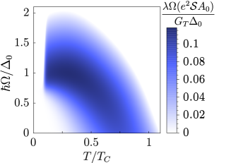
Figure 4: Maximum intrinsic damping, expressed as $\Omega\times\lambda e^{2}\mathcal{S}A_{0}/(G_{T}\Delta_{0})$, for which the system can be refrigerated, with $\bm{h}=-0.3\Delta_{0}\hat{z}$, $P=1$ and Dynes broadening $\Gamma=10^{-5}\Delta_{0}$. The maximum intrinsic damping is determined by solving $A_{0}$ from Eq. (16) with $\delta T=0$.

At higher frequencies the magnetic dissipation, nonlinearities of $\widetilde{\alpha}$ and $\widetilde{G}$, and the coupling between charge and precession start to play a role and limit the attainable temperature difference. For $\mathcal{S}A_{0}/G_{T}=0.1$, the magnitude of the effect is illustrated in Fig. 3. The maximum value of $A_{0}$ for which refrigeration is possible is shown in Fig. 4 as a function of $T$ and $\Omega$. If $\lambda=1$, the parameter regime is similar to that where the spin-torque driven oscillations occur (see Sec. IV.2 below). However, if the intrinsic damping dissipates the energy to systems different from the F conduction electrons ($\lambda<1$), refrigeration is easier to obtain than auto-oscillations. Therefore, measuring the temperature difference $\delta T$ via the thermoelectrically induced voltage $V$ allows for a direct study of the energy dissipation mechanism of the intrinsic Gilbert damping. Note that also in the absence of the spin splitting in S (and therefore $\alpha=0$), it is possible to induce a non-zero voltage via FMR driving Trif and Tserkovnyak (2013). However, that generally requires higher frequencies $\Omega\lesssim\Delta$ than the case analyzed above.

If the thermoelectric coefficient is zero, F always heats up. In the normal state we have

$$\delta T_{\rm normal}=-\frac{G_{T}+8\lambda\mathcal{S}A_{0}}{8G_{\rm th}}\Omega^{2}\theta^{2}<0,$$ (18)

which shows the combined heating effect from the different sources of dissipation. However, in that case the induced voltage $V=0$, and the temperature difference would have to be measured via some other mechanism.

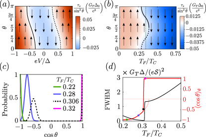
Figure 5: (a) Torque vs. angle $\theta$ and voltage $V$ at $\Omega=0.3\Delta/\hbar$ for $T_{S}=T_{F}=0.5T_{C}$, $\bm{h}=-0.3\Delta_{0}\hat{z}$ and $P=1$. The arrows indicate where the torque drives the angle. The solid black line indicates the stable precession angle $\theta_{*}$, and the dashed line the unstable one. At $V=0$, $\theta_{*}=0$. (b) Torque vs. angle and temperature difference at $\Omega=0.5\Delta/\hbar$ for $T_{S}=0.5T_{C}$, $\bm{h}=0.3\Delta_{0}\hat{z}$, $P=1$, and $V=0$. Moreover, $\mathcal{S}A_{0}=0$. The dashed green line indicates $\delta T_{o}$. (c) Magnetization distribution normalized by its maximum value, for a thermally driven spin oscillator with $\mathcal{S}=100$, $T_{S}=0.5T_{C}$, $\bm{h}=0.3\Delta_{0}\hat{z}$, $P=1$, $V=0$ and $\Omega=0.5\Delta/\hbar$. When $T_{F}\approx 0.31T_{C}$ (dashed line), the distribution is significantly bimodal. (d) Full width at half maximum (FWHM) of the dipole spectrum $S_{xx}(\omega)$ (black line) and the average magnetization (red line) with $G_{T}=e^{2}/\hbar$. The dashed line indicates $\theta_{*}$ and the dots correspond to panel (c).

IV.2 Spin torques

The junction also exhibits a voltage-driven spin torque. With an exchange field such that $\bm{h}\cdot\hat{z}<0$ and $\Omega\lesssim 2h$, the torque due to tunneling becomes antidamping at large voltages. When it exceeds the intrinsic damping, the $\theta=0$ equilibrium configuration is destabilized, and a new stable steady-state configuration $\overline{\tau_{z,\rm tot}(\theta_{*})}=0$ is established. An example of the signs of the torque and the resulting configuration is shown in Fig. 5(a): The stable angle is $\theta_{*}=0$ at small voltages, after which there is a voltage range for which $0<\theta_{*}<\pi$. There, the system realizes a voltage-driven spin oscillator Kiselev et al. (2003); Rippard et al. (2004). At large voltages the stable angle is $\theta_{*}=\pi$, corresponding to a torque-driven magnetization flip.

Similarly, the thermal torque is shown in Fig. 5(b). Due to the nonzero linear-response coupling, it is antisymmetric in small $\delta T$, in contrast to the voltage-driven torque. Consequently, antidamping regions occur for both signs of $\Omega$. In linear response [Eq. (6)], for temperature differences satisfying $\mathop{\mathrm{sgn}}(\alpha)\delta{}T<\delta T_{o}=[1+e^{2}\mathcal{S}A_{0}/(\hbar{}G)]P\hbar\Omega/(2e|\mathfrak{s}|)$, the spin torque drives $\theta\to 0$, damping the precession. Here, $\mathfrak{s}=-P\alpha/(GT)$ is the junction thermopower, which can be $|\mathfrak{s}|\gtrsim{}k_{B}/e$. Ozaeta et al. (2014) Above the critical temperature difference $\delta T_{o}$, the thermal spin torque drives the system away from $\theta_{*}=0$ (or $\theta_{*}=\pi$ for $\Omega<0$). The stable precession angle is shown in Fig. 5(b): there is a range of $\delta T$ in which $\theta_{*}\neq 0,\pi$ and the system exhibits thermally driven Ludwig et al. (2019a) spin oscillations.

In Fig. 5, we neglect the effect of the intrinsic damping $A_{0}$ on the magnetization oscillations. However, it is the main obstacle in reaching auto-oscillations in FMR devices, and we estimate its effect here. For the superconducting systems, generally the effective bias $|\mathfrak{s}|\delta T$ can be at most $\Delta$. Considering the value $\delta T_{o}$ given above, this results to a requirement for the resistance–area product of the S/F junction: $RA\lesssim{}(RA)_{0}=\frac{\hbar\gamma\Delta}{e^{2}A_{0}M_{s}d_{F}|\Omega|}\approx 10^{-4}\,\mathrm{\Omega\,\mu{}m^{2}}\times\frac{1\,\mathrm{T\,nm}\,\Delta}{\mu_{0}M_{s}d_{F}A_{0}|\hbar\Omega|}$, where $d_{F}$ is the ferromagnet thickness. Meeting the requirement is likely challenging. Values $RA\sim 0.1\,\mathrm{\Omega\,\mu{}m^{2}}$ have been achieved in $\sim(100\,\mathrm{nm})^{2}$ lateral size magnetic junctions Kiselev et al. (2003); Nagamine et al. (2006). With such $RA$ and $\mu_{0}M_{s}d_{F}=5\,\mathrm{T\,nm}$ (e.g. Co layer Kiselev et al. (2003)) and $A_{0}=0.01$ Tserkovnyak et al. (2005), the condition is satisfied for $f=|\Omega|/(2\pi)<0.02\Delta/h\approx 1\,\mathrm{GHz}$ (for Al as superconductor). The FMR refrigeration has a similar requirement but with $\Delta\mapsto\Delta/\lambda$, and hence may be easier to achieve, if the microscopic mechanism is such that $\lambda<1$.

V Keldysh action

To properly describe the metastable states in the magnetization precession, we need to extend the formalism. The dynamics beyond average values can be described by an effective action $S=S_{0}+S_{T}$ for the spin including the tunneling, derived Basko and Vavilov (2009); Fransson and Zhu (2008); Zhu et al. (2004); Shnirman et al. (2015); Virtanen and Heikkilä (2017); Ludwig et al. (2017, 2019a, 2019b) by retaining the Keldysh structure Kamenev (2011) for the orientation of the magnetization mean field. The action $S$ describes the generating function of the joint probability distribution $P_{\rm t_{0}}(\delta n,\delta E_{S},\delta E_{F},\delta m_{z})$ [see Eq. (7)], with a source field $\chi$, $\xi_{S}$, $\xi_{F}$, $\zeta$ associated with each of the arguments. The free part reads

$$S_{0}=2\mathcal{S}\int_{-\infty}^{\infty}\mkern-10.0mu\mathrm{d}t\,\left[\left(\frac{\zeta}{2}+\phi^{q}\right)\partial_{t}(\cos\theta)^{c}-(\cos\theta)^{q}(\dot{\phi}^{c}-\Omega)\right]\,,$$ (19)

where $c$ and $q$ denote the symmetric/antisymmetric combinations $x^{c/q}=\frac{x_{+}\pm{}x_{-}}{2}$ of quantities on the two Keldysh branches ($+/-$), for example $(\cos\theta)^{c/q}=\frac{1}{2}[\cos(\theta^{c}+\theta^{q})\pm\cos(\theta^{c}-\theta^{q})]$. Concentrating on slow perturbations around the semiclassical ($\mathcal{S}\gg 1$) precession trajectory $\phi^{c}(t)=\Omega t$, the tunnelling action can be expressed as $S_{T}\simeq{}-i\int_{-\infty}^{\infty}\mathrm{d}t\,s_{T}$ with Virtanen and Heikkilä (2017)

$$s_{T} =\frac{G_{T}}{2}\int_{-\infty}^{\infty}\mathrm{d}\epsilon\,\sum_{\sigma\sigma^{\prime}=\pm}N_{F,\sigma^{\prime}}N_{S,\sigma}\bigl{\{}\frac{\cos\theta^{q}+\sigma\sigma^{\prime}\cos\theta^{c}}{2}$$ (20)

$$\quad\times[e^{i\eta_{\sigma\sigma^{\prime}}}f_{F}(1-f_{S})+e^{-i\eta_{\sigma\sigma^{\prime}}}f_{S}(1-f_{F})]$$

$$\quad-\frac{1+\sigma\sigma^{\prime}(\cos\theta)^{c}}{2}[f_{F}(1-f_{S})+f_{S}(1-f_{F})]\bigr{\}}\,,$$

where $\eta_{\sigma\sigma^{\prime}}=\chi+\epsilon\xi_{S}-(\epsilon-V-\Omega_{\sigma\sigma^{\prime}})\xi_{F}-2\phi^{q}\frac{\Omega_{\sigma\sigma^{\prime}}}{\Omega}$. Here, we have neglected terms that renormalize $\Omega$. For computing time averages, the source fields are taken nonzero between $t=0$ and $t=t_{0}$, e.g. $\chi(t)=\chi\theta(|t_{0}|-|t|)\theta(t\mathop{\mathrm{sgn}}t_{0})$. The results (3–5) can be found as $\overline{I_{c}}=-i\partial_{\chi}s_{T}\rvert_{0}$, $\overline{\dot{E}_{S}}=-i\partial_{\xi_{S}}s_{T}\rvert_{0}$, and $\overline{\tau_{z}}=\frac{1}{2i}\partial_{\phi^{q}}s_{T}\rvert_{0}$, where $\rvert_{0}$ indicates $\phi^{q}=\theta^{q}=\chi=\xi_{S/F}=0$. Expansion around the saddle point gives Eq. (8), and the correlator characterizing the spin torque noise is $D=-\frac{1}{8}\partial_{\phi^{q}}^{2}s_{T}\rvert_{0}\csc^{2}\theta=-\frac{1}{8}\partial_{\theta^{q}}^{2}s_{T}\rvert_{0}$.

V.1 Intrinsic damping

We can include the phenomenological Gilbert damping term $A_{0}\bm{m}\times\dot{\bm{m}}$ of the LLG equation into a corresponding term in the action, $iS_{G}=\int_{-\infty}^{\infty}\mathrm{d}t\,s_{G}(t)$. With the weak-damping assumptions $\dot{\phi}^{c}\simeq\Omega$, $|\dot{\theta}^{c}|\ll|\dot{\phi}|$, the leading term in the torque is produced by $s_{G}\simeq-2i\mathcal{S}A_{0}\Omega\sin^{2}(\theta^{c})\phi^{q}$.

Further reasoning is required for thermodynamic consistency. Let us first assume that the Gilbert damping is caused by a coupling that ultimately dissipates energy into the bath of conduction electrons in F ($\lambda=1$). We can express the conservation of energy in conversion of magnetic energy to energy of conduction electrons as the symmetry $s_{G}[\xi_{F}+x,\phi^{q}+\Omega x/2]=s_{G}[\xi_{F},\phi^{q}]$ for all $x$. In addition, to preserve the thermodynamic fluctuation relations and the second law at equilibrium, the fluctuation symmetry $s_{G}[\xi_{F},\phi^{q}]=s_{G}[iT_{F}^{-1}-\xi_{F},-\phi^{q}]$ should be fulfilled. Virtanen and Heikkilä (2017) The above fixes the series expansion in $\xi_{F}$, $\phi^{q}$, $T_{F}^{-1}$ to have the form

$$s_{G}[\xi_{F},\phi^{q}] \simeq-2A_{0}\mathcal{S}\sin^{2}(\theta^{c})\Bigg{[}i\Omega\left(\phi^{q}-\frac{\Omega}{2}\xi_{F}\right)$$ (21)

$$\qquad+2T_{F}(\phi^{q}-\frac{\Omega}{2}\xi_{F})^{2}\Bigg{]}+\ldots\,.$$

If the Gilbert damping dissipates energy directly to multiple baths (e.g. magnons, phonons), more terms of this form appear, where $\xi_{F}$ and $T_{F}$ should be replaced by the corresponding bath variables, and only a fraction $0\leq\lambda\leq 1$ of the total $A_{0}$ comes from conduction electrons. Including Eq. (21) in the total action $S=S_{0}+S_{T}+S_{G}$ then produces e.g. the correlation function of the Langevin noise terms in Eq. (8), and the additional term in the heat balance equation Eq. (9). These are of course possible to find also directly, by assuming the fluctuation-dissipation theorem, and reasoning about magnetic work done by the damping.

For the external rf drive, we similarly have a term $s_{\rm rf}=2i\mathcal{S}\overline{\bm{m}^{q}\cdot\gamma\bm{h}_{\rm rf}}\simeq 2i\gamma{}h_{\rm rf}\mathcal{S}\sin(\theta^{c})\phi^{q}$, at resonance. It does not obey the above energy conservation symmetry, as power is externally provided and the mechanism generating $h_{\rm rf}$ is not included in the model. As a consequence, as noted in Eq. (12) $\overline{\dot{E}_{S,\rm tot}}+\overline{\dot{E}_{F,\rm tot}}\neq 0$, and the fluctuation relation (7) is modified.

V.2 Spin oscillator

The probability distribution of the magnetization angle $\theta$ can be obtained from Eqs. (19,20) Chudnovskiy et al. (2008); Virtanen and Heikkilä (2017), within a semiclassical method applied to $\tilde{s}_{T}=s_{T}\rvert_{\theta^{q}=\chi=\xi_{j}=0}$ Virtanen and Heikkilä (2017); Kamenev (2011). In this approach, at equilibrium, the fluctuation symmetry $\tilde{s}_{T}(\phi^{q}=-i\Omega/2T)=0$ results to the Boltzmann distribution $P(\cos\theta)=Ne^{\mathcal{S}\cos(\theta)\Omega/T}$. In the nonequilibrium driven state ($V\neq 0$, $\delta{}T\neq 0$), the distribution deviates from this.

The probability distribution is shown in Fig. 5(c) for the thermally driven oscillator. The figure shows the spin torque-driven transition from the magnetization pointing in the direction of the magnetic field ($\cos\theta=1$) for high $T_{F}$, to the opposite direction of the field ($\cos\theta=-1$) at low $T_{F}$. In the intermediate range $T_{F}\approx 0.25$–$0.3T_{c}$, the probability distribution becomes bimodal, reflecting the two locally stable configurations in Fig. 5(b): one of these corresponds to the oscillating state.

V.3 Emission spectrum

A driven spin oscillator produces electromagnetic emission which can be detected. Kiselev et al. (2003); Rippard et al. (2004) This can be characterized with the classical correlator of the magnetic dipole, whose spectrum is approximately a Lorentzian centered at frequency $\Omega$. The classical spectrum of the magnetic dipole correlator can be written as

$$S_{xx}(\omega)=\mathcal{S}^{2}\int_{-\infty}^{\infty}\mathrm{d}t_{0}\,e^{i\omega t_{0}}\langle{m_{x}(t_{0})m_{x}(0)}\rangle\,,$$ (22)

where $m_{x}=\cos\phi\sin\theta$, and the average is over the driven steady state of the system. To evaluate it, the average over $\phi$ can be taken first, noting that $\langle{\cos\phi(t_{0})\cos\phi(0)}\rangle_{\phi}=\frac{1}{2}\mathop{\mathrm{Re}}\langle{e^{i\phi(t_{0})-i\phi(0)}}\rangle_{\phi}=\frac{1}{2}\mathop{\mathrm{Re}}\int\mathrm{D}[\phi^{c},\theta^{q}]\,e^{iS}e^{i\phi^{c}(t_{0})-i\phi^{c}(0)}=\frac{1}{2}\mathop{\mathrm{Re}}\int\mathrm{D}[\phi^{c},\theta^{q}]\,e^{iS^{\prime}}$, where the exponential factor is removed by a shift $(\cos\theta)^{q}\mapsto(\cos\theta)^{q}+\mathop{\mathrm{sgn}}(t_{0})\theta(|t_{0}|-|t|)\theta(t\mathop{\mathrm{sgn}}t_{0})/(2\mathcal{S})$. For $\mathcal{S}\gg 1$, this results to $S^{\prime}-S\simeq\Omega{}t_{0}+i|t_{0}|\mathcal{S}^{-2}D\csc^{2}\theta^{c}=:\psi(t_{0})$ so that $\langle{m_{x}(t_{0})m_{x}(0)}\rangle_{\phi}\simeq\frac{1}{2}\sin^{2}\theta{}\mathop{\mathrm{Re}}{}e^{i\psi(t_{0})}$. Evaluating the Fourier transform, we get

$$S_{xx}(\omega)\simeq\frac{1}{2}\sum_{\pm}\langle{D/[(\omega\pm\Omega)^{2}+(\mathcal{S}^{-2}D\csc^{2}\theta^{c})^{2}]}\rangle_{\theta}\,.$$ (23)

A similar calculation is done in Ref. Chudnovskiy et al., 2008, via Langevin and Fokker–Planck approaches. The remaining average is over the steady state distribution $P(\cos\theta)$.

The linewidth of the spectrum [black line in Fig. 5(d)] in this nonequilibrium system is a non-trivial function of the system parameters. For $T_{F}\approx 0.31T_{C}$ precession at $\theta_{*}$ becomes possible, and as a result the linewidth ($\propto\csc^{2}\theta$) narrows rapidly, becoming significantly smaller than the near-equilibrium fluctuations at $\theta\sim 0,\pi$.

VI Discussion

In this work, we explain how the thermomagnetoelectric effect of a spin-split superconductor couples the magnetization in a magnetic tunnel junction to the temperature difference across it. The thermoelectric coefficient in the superconducting state is generally large, and enables a magnetic Peltier effect and thermal spin torque, with prospects for generating thermally driven oscillations detectable via spectroscopy. Superconductivity also offers possibilities to characterize and control the thermal physics via both the electric and magnetic responses or external field coupling of the magnetization.

Appendix A Tunneling currents

Calculation of the tunneling currents from the model (1) in the main text can be done with standard Green function approaches. Bergeret et al. (2012) Assuming a spin and momentum independent matrix element ($W_{jj^{\prime}}=W$), the $k$-spin component of the spin current to S reads:

$$I_{s}^{k} =\frac{G_{T}}{32}\int_{-\infty}^{\infty}\mathrm{d}\epsilon\,\operatorname{tr}\frac{\sigma_{k}}{2}[(R\check{g}_{F}R^{\dagger})_{+}\check{g}_{S}-\check{g}_{S}(R\check{g}_{F}R^{\dagger})_{-}]^{K},$$ (24)

where the superscript $K$ refers to the Keldysh component and $G_{T}=\pi\nu_{F}\nu_{S}|W|^{2}$ is the normal state tunneling conductance. The charge and energy currents can be obtained by replacing $\sigma_{k}/2\mapsto\hat{\tau}_{3}$ and $\sigma_{k}/2\mapsto\epsilon$ in Eq. (24), respectively. Here, $\sigma_{j}$ and $\hat{\tau}_{j}$ are Pauli matrices in the spin and Nambu spaces, with the basis $(\psi_{\uparrow},\psi_{\downarrow},-\psi_{\downarrow}^{\dagger},\psi_{\uparrow}^{\dagger})$, and $X_{+}(\epsilon,t)=\int\mathrm{d}t^{\prime}\,e^{i\epsilon(t-t^{\prime})}X(t,t^{\prime})$, $X_{-}(\epsilon,t)=\int\mathrm{d}t^{\prime}\,e^{i\epsilon(t^{\prime}-t)}X(t^{\prime},t)$. Moreover, $\check{g}_{F/S}(\epsilon)=\frac{2i}{\pi\nu_{F/S}}\hat{\tau}_{3}\sum_{j}\check{G}_{F/S}(\epsilon,\bm{p}_{j})$ are state-summed Keldysh Green’s functions, normalized by the total density of states (DOS) $\nu_{F/S}$ at Fermi level, of the ferromagnet and the spin-split superconductor. The rotation matrix

$$\begin{split}R=e^{-i\phi\sigma_{z}/2}&e^{-i\theta\sigma_{y}/2}e^{i\phi\sigma_{z}/2}\\ \times\;&e^{-i\int^{t}\mathrm{d}t\,\dot{\phi}(1-\cos\theta)\sigma_{z}/2}e^{-iV\hat{\tau}_{3}t}\end{split}$$ (25)

contains the Euler angles of the time-dependent magnetization direction vector ($\bm{m}\cdot\bm{\sigma}=R\sigma_{z}R^{\dagger}$), a Berry phase factor, and voltage bias $V$. The Berry phase appears from the Green function Flebus et al. (2017); Shnirman et al. (2015) of the conduction electrons in F following adiabatically the changing magnetization. For a metallic ferromagnet, $\hat{g}_{F}^{R}-\hat{g}_{F}^{A}\simeq 2\sum_{\pm}(\hat{\tau}_{3}\pm\sigma_{z})\frac{\nu_{F,\pm}}{\nu_{F}}$ and $\hat{g}^{K}=[\hat{g}^{R}-\hat{g}^{A}](1-2f_{0}(\epsilon))$, where $\nu_{F,\uparrow/\downarrow}:=\nu_{F,\pm}$ are the densities of states of majority/minority spins at the Fermi level and $f_{0}(\epsilon)=(1+e^{\epsilon/T})^{-1}$ is the Fermi distribution function.

Evaluating Eq. (24) for the different currents produces Eqs. (3–5) in the main text, with $N_{S/F,\sigma=\pm}=\frac{1}{2}\operatorname{tr}[\frac{1+\hat{\tau}_{3}}{2}\frac{1+\sigma\sigma_{z}}{2}(\hat{g}_{S/F}^{R}-\hat{g}_{S/F}^{A})]$.

Beyond linear response (6), we find the second-order contributions to the current and torque:

$$\delta^{(2)}\overline{I_{c}} =-\frac{\alpha^{-}_{2,0}}{2}\biggl{[}\sin^{2}(\theta)\Bigl{(}V\Omega-\frac{P\cos\theta}{4}\Omega^{2}\Bigr{)}$$ (26)

$$+P\cos(\theta)V^{2}\biggr{]}-P\cos(\theta)\frac{A}{2}\left(\frac{\delta T}{T}\right)^{2}-B\frac{\delta T}{T}V\,,$$

$$\frac{\delta^{(2)}\overline{\tau_{z}}}{\sin^{2}(\theta)} =\frac{\alpha_{2,0}^{-}}{4}\Bigl{[}V^{2}-P\cos(\theta)V\Omega+\frac{3+\cos(\theta)}{8}\Omega^{2}\Bigr{]}$$ (27)

$$+\frac{A}{4}\biggl{(}\frac{\delta T}{T}\biggr{)}^{2}+\frac{B}{4}\frac{\delta T}{T}\Omega\,,$$

where $\alpha_{i,j}^{\mp}=-(G_{T}/2)\int_{-\infty}^{\infty}\mathrm{d}\epsilon\,\epsilon^{j}{}[N_{S,+}(\epsilon)\mp N_{S,-}(\epsilon)]f_{0}^{(i)}(\epsilon)$, and $A=2\alpha_{1,1}^{-}{+}\alpha_{2,2}^{-}$, $B=\alpha_{1,0}^{+}{+}\alpha_{2,1}^{+}$.

For $\Omega\ll\Delta$, the onset of the voltage driven spin oscillations [Fig. 5(a)] can be determined from Eqs. (6) and (27) to occur at $V_{o}=\pm 4\sqrt{e^{2}\mathcal{S}A_{\rm eff}\Omega/\alpha^{-}_{2,0}}$.

In addition to the spin transfer torque (STT) discussed in the main text, the electron transfer between F and the spin-split S generates also other torque components acting on $F$. This effect can be found from Eq. (24), and appears in the torque components $\overline{\tau_{x/y}}$ perpendicular to the equilibrium magnetization $\hat{z}$.

In the main text, we neglect these torques, because any equilibrium torques can be absorbed to a renormalization of the effective magnetic field, and moreover, in the limit of weak damping and torques the components perpendicular to $\hat{z}$ such that $\tau_{x/y}\ll\mathcal{S}\Omega$ have little effect on the dynamics. In contrast, the component in the main text has a significant effect already at $\overline{\tau_{z}}\sim{}A_{0}\mathcal{S}\Omega\ll\mathcal{S}\Omega$.

For completeness, we write here the expressions for all torques, as obtained from Eq. (24). Equation (5) in the main text gives the dissipative contribution to $\tau_{z}$. Similar contributions can be found for $\tau_{x/y}$:

$$\overline{\tau_{x/y}} =-\frac{G_{T}}{8}\int_{-\infty}^{\infty}\mathrm{d}\epsilon\,\sum_{\sigma\sigma^{\prime}}\frac{(1+\sigma\sigma^{\prime}\cos\theta)^{2}}{2}N_{S,x/y}$$ (28)

$$\qquad\times[f_{F}(\epsilon-\Omega_{\sigma\sigma^{\prime}}-V)-f_{S}(\epsilon)]\,,$$

where $N_{S,0/x/y/z}=\frac{1}{2}\operatorname{tr}\frac{1+\tau_{3}}{2}\frac{\sigma_{0/x/y/z}}{2}(\hat{g}_{S}^{R}-\hat{g}_{S}^{A})$.

In addition, there are two remaining contributions, the equilibrium spin torque, and a Kramers–Kronig counterpart to the density of states term. Terms of the latter type commonly appear in calculations of time-dependent response. To find it, we need $\hat{g}^{R+A}=\hat{g}^{R}+\hat{g}^{A}$. We can evaluate them e.g. in a model with a parabolic spectrum in 3D, $\xi_{k}=k^{2}/(2m)-\mu$. In the superconductor, $h,\Delta\ll\mu_{S}$ and in the magnet, $\Delta=0$. Evaluating the momentum sum yields

$$\hat{g}_{S}^{R+A} \overset{\mu_{S}\to\infty}{\simeq}\hat{g}^{R}_{S,\rm qcl}+\hat{g}^{A}_{S,\rm qcl}+\hat{g}_{F}^{R+A}\rvert_{\bm{h}_{F}\mapsto\bm{h},\mu_{F}\mapsto\mu_{S}}\,,$$ (29)

$$\hat{g}_{F}^{R+A} =2ia\mathop{\mathrm{Re}}\sqrt{-[(\epsilon-h_{F}\sigma_{z})\hat{\tau}_{3}+\mu_{F}]/|\mu_{F}|}+C\,.$$

Here $\hat{g}^{R/A}_{S,\rm qcl}$, are quasiclassical low-energy Green functions Eilenberger (1968), $1/a=\sum_{\pm}\sqrt{1\pm{}h_{F}/\mu_{F}}$, and $h_{F}=\frac{\nu_{F\downarrow}^{2}-\nu_{F\uparrow}^{2}}{\nu_{F\downarrow}^{2}+\nu_{F\uparrow}^{2}}\mu_{F}$ the internal exchange field in F in the model. Moreover, $C$ are scalars independent of $\epsilon$, $\bm{h}$, and $\Delta$, and drop out from expressions for the observables here.

Neglecting terms of order $\Delta/\mu,T/\mu,\Omega/\mu$, we find the remaining terms in the spin current,

$$\bm{I}_{S}^{\prime\prime} =\bm{I}_{S,\rm eq}^{\prime\prime}+\delta\bm{I}_{S}^{\prime\prime}$$ (30)

$$\delta\bm{I}_{S}^{\prime\prime} =-\frac{G_{T}}{64}\int_{-\infty}^{\infty}\mathrm{d}\epsilon\,\sum_{\sigma\sigma^{\prime}}\tanh\frac{\epsilon-\Omega_{\sigma\sigma^{\prime}}-V}{2T_{F}}$$ (31)

$$\qquad\times(\sigma\hat{z}+\sigma^{\prime}\bm{m}(t))\times\bm{P}(\epsilon)N_{F,\sigma^{\prime}}\,,$$

where $\bm{P}(\epsilon)=\frac{1}{2i}\operatorname{tr}\frac{1+\tau_{3}}{2}\bm{\sigma}[\hat{g}^{R}_{S,\rm{}qcl}(\epsilon)+\hat{g}^{A}_{S,\rm{}qcl}(\epsilon)]$. It has the symmetry $\bm{P}(-\epsilon)=\bm{P}(\epsilon)$. For a BCS superconductor, the integrand is nonzero only inside the gap, $|\epsilon\pm{}h|<\Delta$.

The equilibrium spin current $\bm{I}_{S,\rm eq}^{\prime\prime}$ is related to the exchange coupling between F and FI mediated by the electrons in the superconductor. It can be absorbed to a small renormalization of the effective magnetic field acting on F. While its value can be calculated in the above tunneling model, the model is not sufficient for describing this non-Fermi surface term in the realistic situation. The superconducting correction $\delta\bm{I}_{S}^{\prime\prime}$ vanishes at equilibrium, but may contribute to nonequilibrium response. This torque however has $\overline{\tau_{z}^{\prime\prime}}=0$ and can be neglected similarly as in Eq. (28).

Appendix B Adiabatic Green function

In the tunneling calculation of Eq. 24, an expression for the adiabatic Green function of the electrons on the ferromagnet with dynamic magnetization appears. For completeness, we discuss its meaning here. The nonequilibrium Green function for free electrons in a time-dependent exchange field, $H(t)=\sum_{n\sigma\sigma^{\prime}}c^{\dagger}_{n\sigma}[\mathcal{H}_{n}(t)]_{\sigma\sigma^{\prime}}c_{n\sigma^{\prime}}$, $\mathcal{H}_{n}(t)=\epsilon_{n}+\bm{h}(t)\cdot\bm{\sigma}$, with a thermal initial state at $t=0$ is $G_{n}^{>}(t,t^{\prime})=-iU_{n}(t,0)(1-\rho_{n})U_{n}(0,t^{\prime})^{\dagger}$, where $i\partial_{t}U_{n}(t,t^{\prime})=[\epsilon_{n}-\bm{h}(t)\cdot\bm{\sigma}]U_{n}(t,t^{\prime})$, $U(t,t)=1$, and $\rho_{n}=[1+e^{\mathcal{H}_{n}(0)/T}]^{-1}$. In an adiabatic approximation for $|\dot{h}|\ll{}h^{2}$, $U_{n}(t,t^{\prime})\simeq{}e^{-i(t-t^{\prime})\epsilon_{n}}R(t)e^{i\varphi_{n}(t,t^{\prime})\sigma_{z}/2}R(t^{\prime})^{\dagger}$, where $R(t)\sigma_{z}R(t)^{\dagger}=\bm{h}(t)\cdot\bm{\sigma}$ and $\varphi_{n}(t,t^{\prime})=i\int_{t^{\prime}}^{t}\mathrm{d}t^{\prime\prime}\,\operatorname{tr}\sigma_{z}R(t^{\prime\prime})^{\dagger}\partial_{t^{\prime\prime}}R(t^{\prime\prime})$. In terms of Euler angles $\bm{h}=(\cos\phi\sin\theta,\sin\phi\sin\theta,\cos\theta)$ we write $R=e^{-i\phi\sigma_{z}/2}e^{-i\theta\sigma_{y}/2}e^{i\phi\sigma_{z}/2}e^{-i\chi\sigma_{z}/2}$. The function $\chi(t)$ is arbitrary, but $U_{n}$ does not depend on it. For simplicity, we choose $\chi=\int^{t}\mathrm{d}t^{\prime}\,\dot{\phi}(1-\cos\theta)$, which gives $\varphi_{n}=0$. With this choice, the adiabatic Green function becomes

$$G^{>}_{n}(t,t^{\prime})=R(t)G_{n,0}^{>}(t-t^{\prime})R(t^{\prime})^{\dagger}\,,$$ (32)

and the electron Berry phase appears only in the rotation matrix. This is equivalent to the “rotating frame” picture used in the main text and other works Tserkovnyak et al. (2005, 2008).