Are SonarQube Rules Inducing Bugs?

Abstract

Background. The popularity of tools for analyzing Technical Debt, and particularly the popularity of SonarQube, is increasing rapidly. SonarQube proposes a set of coding rules, which represent something wrong in the code that will soon be reflected in a fault or will increase maintenance effort. However, our local companies were not confident in the usefulness of the rules proposed by SonarQube and contracted us to investigate the fault-proneness of these rules.
Objective. In this work we aim at understanding which SonarQube rules are actually fault-prone and to understand which machine learning models can be adopted to accurately identify fault-prone rules.
Method. We designed and conducted an empirical study on 21 well-known mature open-source projects. We applied the SZZ algorithm to label the fault-inducing commits. We analyzed the fault-proneness by comparing the classification power of seven machine learning models.
Result. Among the 202 rules defined for Java by SonarQube, only 25 can be considered to have relatively low fault-proneness. Moreover, violations considered as ”bugs” by SonarQube were generally not fault-prone and, consequently, the fault-prediction power of the model proposed by SonarQube is extremely low.
Conclusion. The rules applied by SonarQube for calculating technical debt should be thoroughly investigated and their harmfulness needs to be further confirmed. Therefore, companies should carefully consider which rules they really need to apply, especially if their goal is to reduce fault-proneness.

I Introduction

The popularity of tools for analyzing technical debt, such as SonarQube, is increasing rapidly. In particular, SonarQube has been adopted by more than 85K organizations  including nearly 15K public open-source projects . SonarQube analyzes code compliance against a set of rules. If the code violates a rule, SonarQube adds the time needed to refactor the violated rule as part of the technical debt. SonarQube also identifies a set of rules as ”bugs”, claiming that they ”represent something wrong in the code and will soon be reflected in a fault”; moreover, they also claim that zero false positives are expected from ”bugs” .

Four local companies have been using SonarQube for more than five years to detect possible issue in their code, reported that their developers do not believe that the rules classified as bugs can actually result in faults. Moreover, they also reported that the manual customization of the SonarQube out-of-the-box set of rules (named ”the Sonar way”) is very subjective and their developers did not manage to agree on a common set of rules that should be enforced. Therefore, the companies asked us to understand if it is possible to use machine learning to reduce the subjectivity of the customization of the SonarQube model, considering only rules that are actually fault-prone in their specific context.

SonarQube is not the most used static analysis tool on the market. Other tools such as Checkstyle, PMD and FindBugs are more used, especially in Open Source Projects [1] and in research [2]. However, the adoption of another tool in the DevOps pipeline requires extra effort for the companies, including the training and the maintenance of the tool itself. If the SonarQube rules actually resulted fault-prone, our companies would not need to invest extra effort to adopt and maintain other tools.

At the best of our knowledge, not studies have investigated the fault-proneness of SonarQube rules, and therefore, we accepted the challenge and we designed and conducted this study. At best, only a limited number of studies have considered SonarQube rule violations [3], [4], but they did not investigate the impact of the SonarQube violations considered as ”bugs” on faults.

The goal of this work is twofold:

• Analyze the fault-proneness of SonarQube rule violations, and in particular, understand if rules classified as ”bugs” are more fault-prone than security and maintainability rules.

• Analyze the accuracy of the quality model provided by SonarQube in order to understand the fault-prediction accuracy of the rules classified as ”bugs”.

SonarQube and issue tracking systems adopt similar terms for different concepts. Therefore, in order to clarify the terminology adopted in this work, we define  SQ-Violation as a violated SonarQube rule that generated a SonarQube ”issue” and fault as an incorrect step, process, data definition, or any unexpected behavior in a computer program inserted by a developer, and reported by Jira issue-tracker. We also use the term ”fault-fixing” commit for commits where the developers have clearly reported bug fixing activity and ”fault-inducing” commits for those commits that are responsible for the introduction of a fault.

The remainder of this paper is structured as follows. In Section II-A we introduce SonarQube and the SQ-Violations adopted in this work. In Section II we present the background of this work, introducing the SonarQube violations and the different machine learning algorithms applied in this work. In Section III, we describe the case study design. Section IV presents respectively the obtained results. Section V identifies threats to validity while Section VI describes related works. Finally, conclusions are drawn in Section VII.

II Background

II-A SonarQube

SonarQube is one of the most common Open Source static code analysis tools adopted both in academia [5],[2] and in industry [1]. SonarQube is provided as a service from the sonarcloud.io platform or it can be downloaded and executed on a private server.

SonarQube calculates several metrics such as the number of lines of code and the code complexity, and verifies the code’s compliance against a specific set of ”coding rules” defined for most common development languages. In case the analyzed source code violates a coding rule or if a metric is outside a predefined threshold, SonarQube generates an ”issue”. SonarQube includes Reliability, Maintainability and Security rules.

Reliability rules, also named ”bugs” create issues (code violations) that ”represents something wrong in the code” and that will soon be reflected in a bug. ”Code smells” are considered ”maintainability-related issues” in the code that decreases code readability and code modifiability. It is important to note that the term ”code smells” adopted in SonarQube does not refer to the commonly known code smells defined by Fowler et al. [6] but to a different set of rules. Fowler et al. [6] consider code smells as ”surface indication that usually corresponds to a deeper problem in the system” but they can be indicators of different problems (e.g., bugs, maintenance effort, and code readability) while rules classified by SonarQube as ”Code Smells” are only referred to maintenance issues. Moreover, only four of the 22 smells proposed my Fowler et al. are included in the rules classified as ”Code Smells” by SonarQube (Duplicated Code, Long Method, Large Class, and Long Parameter List).

SonarQube also classifies the rules into five severity levels: Blocker, Critical, Major, Minor, and Info.

In this work, we focus on the sq-violations, which are reliability rules classified as ”bugs” by SonarQube, as we are interested in understanding whether they are related to faults.

SonarQube includes more than 200 rules for Java (Version 6.4). In the replication package (Section III-D) we report all the violations present in our dataset. In the remainder of this paper, column ”squid” represents the original rule-id (SonarQube ID) defined by SonarQube. We did not rename it, to ease the replicability of this work. In the remainder of this work, we will refer to the different sq-violations with their id (squid). The complete list of violations can be found in the file ”SonarQube-rules.xsls” in the online raw data.

II-B Machine Learning Techniques

In this Section, we describe the machine learning techniques adopted in this work to predict the fault-proneness of sq-violations. Due to the nature of the task, all the models used for this work were used for classification. We compared eight machine learning models. Among these, we used a generalized linear model: Logistic Regression [7]; one tree based classifier: Decision Tree [8]; and 6 ensemble classifiers: Bagging [9], Random Forest [10], Extremely Randomized Trees [11], AdaBoost [12], Gradient Boosting [13], and XGBoost [14] which is an optimized implementation of Gradient Boosting. All the models, except the XGBoost, were implemented using the library Scikit-Learn, applying the default parameters for building the models. For the ensamble classifiers we alwasys used 100 estimators. The XGBoost classifier was implemented using the XGBoost library also trained with 100 estimators.

II-B1 Logistic Regression [7]

Contrary to the linear regression, which is used to predict a numerical value, Logistic Regression is used for predicting the category of a sample. Particularly, a binary Logistic Regression model is used to estimate the probability of a binary result ($0$ or $1$) given a set of independent variables. Once the probabilities are known, these can be used to classify the inputs in one of the two classes, based on their probability to belong to either of the two.

Like all linear classifiers, Logistic Regression projects the $P$-dimensional input $\bf x$ into a scalar by a dot product of the learned weight vector ${\bf w}$ and the input sample: ${\bf w}\cdot{\bf x}+w_{0}$, where $w_{0}\in\mathbb{R}$ the constant intercept. To have a result which can be interpreted as a class membership probability—a number between $0$ and $1$—Logistic Regression passes the projected scalar through the logistic function (sigmoid). This function, for any given input $x$, returns an output value between $0$ and $1$. The logistic function is defined as

$$\sigma(x)=\frac{1}{1+e^{-x}}.$$

Where the class probability of a sample ${\bf x}\in\mathbb{R}^{P}$ is modeled as

$$Pr(c=1\mid{\bf x})=\frac{1}{1+e^{-({\bf w}\cdot{\bf x}+w_{0})}}.$$

Logistic Regression is trained through maximum likelihood: the model’s parameters are estimated in a way to maximize the likelihood of observing the inputs with respect to the parameters $\bf w$ and $w_{0}$. We chose to use this model as baseline as it requires limited computational resources and it is easy to implement and fast to train.

II-B2 Decision Tree Classifier [8]

Utilizes a decision tree to return an output given a series of input variables. Its tree structure is characterized by a root node and multiple internal nodes, which are represented by the input variable, and leaf, corresponding to the output. The nodes are linked between one another through branches, representing a test. The output is given by the decision path taken. A decision tree is structured as a if-then-else diagram: in this structure, given the value of the variable in the root node, it can lead to subsequent nodes through branches following the result of a test. This process is iterated for all the input variables (one for each node) until it reaches the output, represented by the leaves of the tree.

In order to create the best structure, assigning each input variable to a different node, a series of metrics can be used. Amongst these we can find the GINI impurity and the information gain:

• Gini impurity measures how many times randomly chosen inputs would be wrongly classified if assigned to a randomly chosen class;

• Information gain measures how important is the information obtained at each node related to its outcome: the more important is the information obtained in one node, the purer will be the split.

In our models we used the Gini impurity measure to generate the tree as it is more computationally efficient. The reasons behind the choice of decision tree models and Logistic Regression, are their simplicity and easy implementation. Moreover, the data does not need to be normalized, and the structure of the tree can be easily visualized. However, this model is prone to overfitting, and therefore it cannot generalize the data. Furthermore, it does not perform well with imbalanced data, as it generates a biased structure.

II-B3 Random Forest [10]

is an ensemble technique that helps to overcome overfitting issues of the decision tree. The term ensemble indicates that these models use a set of simpler models to solve the assigned task. In this case, Random Forest uses an ensemble of decision trees.

An arbitrary number of decision trees is generated considering a randomly chosen subset of the samples of the original dataset [9]. This subset is created with replacement, hence a sample can appear multiple times. Moreover, in order to reduce the correlation between the individual decision trees a random subset of the features of the original dataset. In this case, the subset is created without replacement. Each tree is therefore trained on its subset of the data, and it is able to give a prediction on new unseen data. The Random Forest classifier uses the results of all these trees and averages them to assign a label to the input. By randomly generating multiple decision trees, and averaging their results, the Random Forest classifier is able to better generalize the data. Moreover, using the random subspace method, the individual trees are not correlated between one another. This is particularly important when dealing with a dataset with many features, as the probability of them being correlated between each other increases.

II-B4 Bagging [9]

Exactly like the Random Forest model, the Bagging classifier is applied to an arbitrary number of decision trees which are constructed choosing a subset of the samples of the original dataset. The difference with the Random Forest classifier is in the way in which the split point is decided: while in the Random Forest algorithm the splitting point is decided base on a random subset of the variables, the Bagging algorithm is allowed to look at the full set of variable to find the point minimizing the error. This translates in structural similarities between the trees which do not resolve the overfitting problem related to the single decision tree. This model was included as a mean of comparison with newer and better performing models.

II-B5 Extremely Randomized Trees [11]

(ExtraTrees) [11], provides a further randomization degree to the Random Forest. For the Random Forest model, the individual trees are created by randomly choosing subsets of the dataset features. In the ExtraTrees model the way each node in the individual decision trees are split is also randomized. Instead of using the metrics seen before to find the optimal split for each node (Gini impurity and Information gain), the cut-off choice for each node is completely randomized, and the resulting splitting rule is decided based on the best random split. Due to its characteristics, especially related to the way the splits are made at the node level, the ExtraTrees model is less computationally expensive than the Random Forest model, while retaining a higher generalization capability compared to the single decision trees.

II-B6 AdaBoost [12]

is another ensemble algorithm based on boosting [15] where the individual decision trees are grown sequentially. Moreover, a weight is assigned to each sample of the training set. Initially, all the samples are assigned the same weight. The model trains the first tree in order to minimize the classification error, and after the training is over, it increases the weights to those samples in the training set which were misclassified. Moreover, it grows another tree and the whole model is trained again with the new weights. This whole process continues until a predefined number of trees has been generated or the accuracy of the model cannot be improved anymore. Due to the many decision trees, as for the other ensemble algorithms, AdaBoost is less prone to overfitting and can, therefore, generalize better the data. Moreover, it automatically selects the most important features for the task it is trying to solve. However, it can be more susceptible to the presence of noise and outliers in the data.

II-B7 Gradient Boosting [13]

also uses an ensemble of individual decision trees which are generated sequentially, like for the AdaBoost. The Gradient Boosting trains at first only one decision tree and, after each iteration, grows a new tree in order to minimize the loss function. Similarly to the AdaBoost, the process stops when the predefined number of trees has been created or when the loss function no longer improves.

II-B8 XGBoost [14]

can be viewed as a better performing implementation of the Gradient Boosting algorithm, as it allows for faster computation and parallelization. For this reason it can yield better performance compared to the latter, and can be more easily scaled for the use with high dimensional data.

III Case Study Design

We designed our empirical study as a case study based on the guidelines defined by Runeson and H’́ost [16]. In this Section, we describe the empirical study including the goal and the research questions, the study context, the data collection and the data analysis.

III-A Goal and Research Questions

As reported in Section 1, our goals are to analyze the fault-proneness of SonarQube rule violations (SQ-Violations) and the accuracy of the quality model provided by SonarQube. Based on the aforementioned goals, we derived the following three research questions (RQs).

RQ1	Which are the most fault-prone SQ-Violations?
	In this RQ, we aim to understand whether the introduction of a set of SQ-Violations is correlated with the introduction of faults in the same commit and to prioritize the SQ-Violations based on their fault-proneness.
	Our hypothesis is that a set of SQ-Violations should be responsible for the introduction of bugs.
RQ2	Are SQ-Violations classified as ”bugs” by SonarQube more fault-prone than other rules?
	Our hypothesis is that reliability rules (”bugs”) should be more fault-prone that maintainability rules (”code smells”) and security rules.
RQ3	What is the fault prediction accuracy of the SonarQube quality model based on violations classified as ”bugs”?
	SonarQube claims that whenever a violation is classified as a ”bug”, a fault will develop in the software.
	Therefore, we aim at analyzing the fault prediction accuracy of the rules that are classified as ”bugs” by measuring their precision and recall.

III-B Study Context

In agreement with the four companies, we considered open source projects available in the Technical Debt Dataset [17]. The reason for considering open source projects instead of their private projects is that not all the companies would have allowed us to perform an historical analysis of all their commits. Moreover, with closed source projects the whole process cannot be replicated and verified transparently.

For this purpose, the four companies selected together 21 out of 31 projects available, based on the ones that were more similar to their internal projects considering similar project age, size, usage of patterns used and other criteria that we cannot report for reason of NDA.

The dataset includes the analysis of each commit of the projects from their first commit until the end of 2015 with SonarQube, information on all the Jira issues, and a classification of the fault-inducing commits performed with the SZZ algorithm [18].

In Table I, we report the list of projects we considered together with the number of analyzed commits, the project size (LOC) of the last analyzed commits, the number of faults identified in the selected commits, and the total number of SQ-Violations.

TABLE I: The selected projects

Project Name	Analyzed commits	Last commit LOC	Faults	SonarQube Violations
Ambari	9727	396775	3005	42348
Bcel	1255	75155	41	8420
Beanutils	1155	72137	64	5156
Cli	861	12045	59	37336
Codec	1644	34716	57	2002
Collections	2847	119208	103	11120
Configuration	2822	124892	153	5598
Dbcp	1564	32649	100	3600
Dbutils	620	15114	21	642
Deamon	886	3302	4	393
Digester	2132	43177	23	4945
FileUpload	898	10577	30	767
Io	1978	56010	110	4097
Jelly	1914	63840	45	5057
Jexl	1499	36652	58	34802
Jxpath	596	40360	43	4951
Net	2078	60049	160	41340
Ognl	608	35085	15	4945
Sshd	1175	139502	222	8282
Validator	1325	33127	63	2048
Vfs	1939	59948	129	3604
Sum	39.518	1,464,320	4,505	231,453

III-C Data Analysis

Before answering our RQs, we first executed the eight machine learning (ML) models, we compared their accuracy, and finally performed the residual analysis.

The next subsections describe the analysis process in details as depicted in Figure 1.

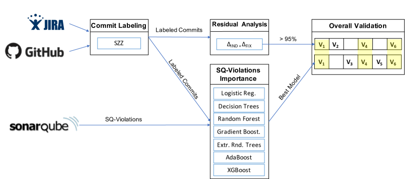
Figure 1: The Data Analysis Process

III-C1 Machine Learning Execution

In this step we aim at comparing fault-proneness prediction power of SQ-Violations by applying the eight machine learning models described in Section II-B.

Therefore we aim at predicting the fault-proneness of a commit (labeled with the SZZ algorithm) by means of the SQ-Violations introduced in the same commit. We used the SQ-Violations introduced in each commits as independent variables (predictors) to determine if a commit is fault-inducing (dependent variable).

After training the eight models described in Section II-B, we performed a second analysis retraining the models using a drop-column mechanism [19]. This mechanism is a simplified variant of the exhaustive search [20], which iteratively tests every subset of features for their classification performance. The full exhaustive search is very time-consuming requiring $2^{P}$ train-evaluation steps for a $P$-dimensional feature space. Instead, we look only at dropping individual features one at a time, instead of all possible groups of features.

More specifically, a model is trained $P$ times, where $P$ is the number of features, iteratively removing one feature at a time, from the first to the last of the dataset. The difference in cross-validated test accuracy between the newly trained model and the baseline model (the one trained with the full set of features) defines the importance of that specific feature. The more the accuracy of the model drops, the more important for the classification is the specific feature.

The feature importance of the SQ-Violation has been calculated for all the machine learning models described, but we considered only the importance calculated by the most accurate model (cross-validated with all $P$ features, as described in the next section), as the feature importances of a poor classifier are likely to be less reliable.

III-C2 Accuracy Comparison

Apart from ranking the SQ-Violations by their importance, we first need to confirm the validity of the prediction model. If the predictions obtained from the ML techniques are not accurate, the feature ranking would also become questionable. To assess the prediction accuracy, we performed a 10-fold cross-validation, dividing the data in 10 parts, i.e., we trained the models ten times always using 1/10 of the data as a testing fold. For each fold, we evaluated the classifiers by calculating a number of accuracy metrics (see below). The data related to each project have been split in 10 sequential parts, thus respecting the temporal order, and the proportion of data for each project. The models have been trained iteratively on group of data preceding the test set. The temporal order was also respected for the groups included in the training set: as an example, in fold 1 we used group 1 for training and group 2 for testing, in fold 2 groups 1 and 2 were used for training and group 3 for testing, and so on for the remaining folds.

As accuracy metrics, we first calculated precision and recall. However, as suggested by  [21], these two measures present some biases as they are mainly focused on positive examples and predictions and they do not capture any information about the rates and kind of errors made.

The contingency matrix (also named confusion matrix), and the related f-measure help to overcome this issue. Moreover, as recommended by [21], the Matthews Correlation Coefficient (MCC) should be also considered to understand possible disagreement between actual values and predictions as it involves all the four quadrants of the contingency matrix.

From the contingency matrix, we retrieved the measure of true negative rate (TNR), which measures the percentage of negative sample correctly categorized as negative, false positive rate (FPR) which measures the percentage of negative sample misclassified as positive, and false negative rate (FNR), measuring the percentage of positive samples misclassified as negative. The measure of true positive rate is left out as equivalent to the recall. The way these measures were calculated can be found in Table II.

TABLE II: Accuracy Metrics Formulae

Accuracy Measure	Formula
Precision	$\frac{TP}{FP+TP}$
Recall	$\frac{TP}{FN+TP}$
MCC	$\frac{TP*TN-FP*FN}{\sqrt{(FP+TP)(FN+TP)(FP+TN)(FN+TN)}}$
f-measure	$2*\frac{precision*recall}{precision+recall}$
TNR	$\frac{TN}{FP+TNe}$
FPR	$\frac{FP}{TN+FP}$
FNR	$\frac{FN}{FN+TP}$

TP: True Positive; TN: True Negative; FP: False Positive; FN: False Negative

Finally, to graphically compare the true positive and the false positive rates, we calculated the Receiver Operating Characteristics (ROC), and the related Area Under the Receiver Operating Characteristic Curve (AUC): the probability that a classifier will rank a randomly chosen positive instance higher than a randomly chosen negative one.

In our dataset, the proportion of the two types of commits is not even: a large majority (approx. 90 %) of the commits were non-fault-inducing, and a plain accuracy score would reach high values simply by always predicting the majority class. On the other hand, the ROC curve (as well as the precision and recall scores) are informative even in seriously unbalanced situations.

III-C3 SQ-Violations Residual Analysis

The results from the previous ML techniques show a set of SQ-Violations related with fault-inducing commits. However, the relations obtained in the previous analysis do not imply causation between faults and SQ-Violations.

In this step, we analyze which violations were introduced in the fault-inducing commits and then removed in the fault-fixing commits. We performed this comparison at the file level. Moreover, we did not consider cases where the same violation was introduced in the fault-inducing commit, removed, re-introduced in commits not related to the same fault, and finally removed again during the fault-fixing commit.

In order to understand which SQ-Violations were introduced in the fault-inducing commits (IND) and then removed in the fault-fixing commit (FIX), we analyzed the residuals of each SQ-Violation by calculating:

$$Residual=\Delta_{IND}+\Delta_{FIX}$$

where $\Delta_{IND}$ and $\Delta_{FIX}$ are calculated as:

$\Delta_{IND}$ = #SQ-Violations introduced in the fault-inducing commit

$\Delta_{FIX}$ =#SQ-Violations removed in the fault-fixing commit

Figure 2 schematizes the residual analysis.

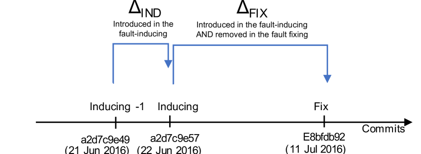
Figure 2: Residuals Analysis

We calculated the residuals for each commit/fix pair, verifying the introduction of the SQ-Violation $V_{i}$ in the fault-inducing commit (IND) and the removal of the violation in the fault-fixing commit (FIX). If $\Delta_{IND}$ was lower than zero, no SQ-Violations were introduced in the fault-inducing commit. Therefore, we tagged such a commit as not related to faults.

For each violation, the analysis of the residuals led us to two groups of commits:

• Residual $>$ 0: The SQ-Violations introduced in the fault-inducing commits were not removed during the fault-fixing.

• Residual $\leq$ 0: All the SQ-Violations introduced in the fault-inducing commits were removed during the fault-fixing. If Residual $<$ 0, other SQ-Violations of the same type already present in the code before the bug-inducing commit were also removed.

For each SQ-Violations, we calculated descriptive statistics so as to understand the distribution of residuals.

Then, we calculated the residual sum of squares (RSS) as:

$$RSS=\displaystyle\sum(Residual)^{2}$$

We calculated the percentage of residuals equal to zero as:

$$\frac{\#zero\_residuals}{\#residuals}*100\%$$

Based on the residual analysis, we can consider violations where the percentage of zero residuals was higher than 95% as a valid result.

III-C4 RQ1: Which are the most fault-prone SQ-Violations?

In order to analyze RQ1, we combined the results obtained from the best ML technique and from the residual analysis. Therefore, if a violation has a high correlation with faults but the percentage of the residual is very low, we can discard it from our model, since it will be valuable only in a limited number of cases. As we cannot claim a cause-effect relationship without a controlled experiment, the results of the residual analysis are a step towards the identification of this relationship and the reduction of spurious correlations.

III-C5 RQ2: Are SQ-Violations classified as ”bugs” by Sonar-Qube more fault-prone than other rules?

The comparison of rules classified as ”bugs” with other rules has been performed considering the results of the best ML techniques and the residual analysis, comparing the number of violations classified as ”bug” that resulted to be fault-prone from RQ1. We expect bugs to be in the most faults-prone rules.

III-C6 RQ3: What is the fault prediction accuracy of the SonarQube quality model based on violations classified as ”bugs”

Since SonarQube considers every SQ-Violation tagged as a ”bug” as ”something wrong in the code that will soon be reflected in a bug”, we also analyzed the accuracy of the model provided by SonarQube.

In order to answer our RQ3, we calculated the percentage of SQ-Violations classified as ”bugs” that resulted in being highly fault-prone according to the previous analysis. Moreover, we also analyzed the accuracy of the model calculating all the accuracy measures reported in Section III-C2.

III-D Replicability

In order to allow the replication of our study, we published the raw data in the replication package .

IV Results

In this work, we considered more than 37 billion effective lines of code and retrieved a total of 1,464,320 violations from 39,518 commits scanned with SonarQube. Table 1 reports the list of projects together with the number of analyzed commits and the size (in Lines of Code) of the latest analyzed commit. We retrieved a total of 4,505 faults reported in the issue trackers.

All the 202 rules available in SonarQube for Java were found in the analyzed projects. For reasons of space limitations, we will refer to the SQ-Violations only with their SonarQube id number (SQUID). The complete list of rules, together with their description is reported in the online replication package (file SonarQube-rules.xlsx). Note that in column ”Type” MA means Major, Mi means Minor, CR means Critical, and BL means Blocker.

IV-A RQ1: Which are the most fault-prone SQ-Violations?

In order to answer this RQ, we first analyzed the importance of the SQ-Violations by means of the most accurate ML technique and then we performed the residual analysis.

IV-A1 SQ-Violations Importance Analysis

As shown in Figure 3, XGBoost resulted in the most accurate model among the eight machine learning techniques applied to the dataset. The 10-fold cross-validation reported an average AUC of 0.83. Table III (column RQ1) reports average reliability measures for the eight models.

Despite the different measures have different strengths and weaknesses (see Section III-C2), all the measures are consistently showing that XGBoost is the most accurate technique.

The ROC curves of all models are depicted in Table III while the reliability results of all the 10-folds models are available in the online replication package.

Therefore, we selected XGBoost as classification model for the next steps, and utilized the feature importance calculated applying the drop-column method to this classifier. The XGBoost classifier was retrained removing one feature at a time sequentially.

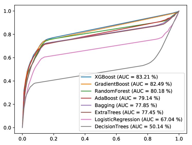
Figure 3: ROC Curve (Average between 10-fold validation models)

TABLE III: Model Reliability

	RQ1 (Average between 10-fold validation models)							RQ2	RQ3
Measure	Logistic Regr.	Decision Tree	Bagging	Random Forest	Extra Trees	AdaBoost	Gradient Boosting	XGBoost	SQ ”bugs”
Precision	0.417	0.311	0.404	0.532	0.427	0.481	0.516	0.608	0.086
Recall	0.076	0.245	0.220	0.156	0.113	0.232	0.192	0.182	0.028
MCC	0.162	0.253	0.279	0.266	0.203	0.319	0.300	0.318	0.032
f-measure	0.123	0.266	0.277	0.228	0.172	0.301	0.275	0.275	0.042
TNR	0.996	0.983	0.990	0.995	0.995	0.993	0.995	0.997	0.991
FPR	0.004	0.002	0.010	0.004	0.005	0.007	0.005	0.003	0.009
FNR	0.924	0.755	0.779	0.844	0.887	0.768	0.808	0.818	0.972
AUC	0.670	0.501	0.779	0.802	0.775	0.791	0.825	0.832	0.509

23 SQ-Violations have been ranked with an importance higher than zero by the XGBoost. In Table VI, we report the SQ-Violations with an importance higher or equal than 0.01 % (coloumn ”Intr. & Rem. (%)” reports the number of violations introduced in the fault-inducing commits AND removed in the fault-fixing commits). The remaining SQ-Violations are reported in the raw data for reasons of space. coloumn ”Intr. & Rem. (%)” means

The combination of the 23 violations guarantees a good classification power, as reported by the AUC of 0.83. However, the drop column algorithm demonstrates that SQ-Violations have a very low individual importance. The most important SQ-Violation has an importance of 0.62%. This means that the removal of this variable from the model would decrease the accuracy (AUC) only by 0.62%. Other three violations have a similar importance (higher than 0.5%) while others are slightly lower.

IV-A2 Model Accuracy Validation

The analysis of residuals shows that several SQ-Violations are introduced in fault-inducing commits in more than 50% of cases. 32 SQ-Violations out of 202 had been introduced in the fault-inducing commits and then removed in the fault-fixing commit in more than 95% of the faults. The application of the XGBoost, also confirmed an importance higher than zero in 26 of these SQ-Violations. This confirms that developers, even if not using SonarQube, pay attention to these 32 rules, especially in case of refactoring or bug-fixing.

Table VI reports the descriptive statistics of residuals, together with the percentage residuals = 0 (number of SQ-Violations introduced during fault-inducing commits and

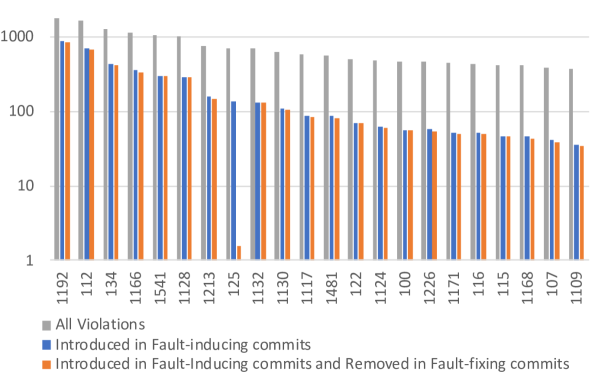
Figure 4: Comparison of Violations introduced in fault-inducing commits and removed in fault-fixing commits

removed during fault-fixing commits).

Column ”Res $>$95%”, shows a checkmark (✓) when the percentage of residuals=0 was higher than 95%.

Figure 4 compares the number of violations introduced in fault-inducing commits, and the number of violations removed in the fault-fixing commits.

IV-B Manual Validation of the Results

In order to understand the possible causes and to validate the results, we manually analyzed 10 randomly selected instances for the first 20 SQ-Violations ranked as more important by the XGBoost algorithm.

The first immediate result is that, in 167 of the 200 manually inspected violations, the bug induced in the fault-inducing commit was not fixed by the same developer that induced it.

We also noticed that violations related to duplicated code and empty statements (eg. ”method should not be empty”) always generated a fault (in the randomly selected cases). When committing an empty method (often containing only a ”TODO” note), developers often forgot to implement it and then used it without realizing that the method did not return the expected value. An extensive application of unit testing could definitely reduce this issue. However, we are aware that is is a very common practice in several projects. Moreover, SQ-Violations such as 1481 (unused private variable should be removed) and 1144 (unused private methods should be removed) unexpectedly resulted to be an issue. In several cases, we discovered methods not used, but expected to be used in other methods, resulted in a fault. As example, if a method A calls another method B to compose a result message, not calling the method B results in the loss of the information provided by B.

IV-C RQ2: Are SQ-Violations classified as ”bugs” by SonarQube more fault-prone than other rules?

Out of the 57 violations classified as ”bugs” by SonarQube, only three (squid 1143, 1147, 1764) were considered fault-prone with a very low importance from the XGBoost and with residuals higher than 95%. However, rules classified as ”code smells” were frequently violated in fault-inducing commits. However, considering all the SQ-Violations, out of 40 the SQ-Violations that we identified as fault-prone, 37 are classified as ”code smells” and one as security ”vulnerability”.

When comparing severity with fault proneness of the SQ-Violations, only three SQ-Violations (squid 1147, 2068, 2178) were associated with the highest severity level (blocker). However, the fault-proneness of this rule is extremely low (importance $<$= 0.14%). Looking at the remaining violations, we can see that the severity level is not related to the importance reported by the XGBoost algorithm since the rules of different level of severity are distributed homogeneously across all importance levels.

IV-D RQ3: Fault prediction accuracy of the SonarQube model

”Bug” violations were introduced in 374 commits out of 39,518 analyzed commits. Therefore, we analyzed which of these commits were actually fault-inducing commits. Based on SonarQube’s statement, all these commits should have generated a fault.

All the accuracy measures (Table III, column ”RQ2”) confirm the very low prediction power of ”bug” violations. The vast majority of ”bug” violations never become a fault. Results are also confirmed by the extremely low AUC (50.95%) and by the contingency matrix (Table IV). The results of the SonarQube model also confirm the results obtained in RQ2. Violations classified as ”bugs” should be classified differently since they are hardly ever injected in fault-inducing commits.

TABLE IV: SonarQube Contingency Matrix (Prediction model based on SQ-Violations considered as ”Bug” by SonarQube)

	Predicted	Actual
		IND	NOT IND
	IND	32	342
	NOT IND	1,124	38,020

TABLE V: Summary of the most important SonarQube Violations Related to Faults (XGBoost Importance $>$ 0.2%)

SonarQube				SZZ		Residuals					XG Boost	Res. $>$95%
SQUID	Severity	Type	# Occ.	Intr. & Rem.(%)	Intr. in fault-ind	Mean	Max	Min	Stdev	RSS	Imp.
S1192	CRITICAL	CS	1815	50,87	95,10	245,60	-861	2139	344,42	1726	0,66	✓
S1444	MINOR	CS	96	2,69	97,92	4,59	-7	73	10,34	94	0,62	✓
Useless Import Check	MAJOR	CS	1026	28,76	97,27	33,37	-170	351	61,58	998	0,41	✓
S00105	MINOR	CS	263	7,37	97,72	1,96	-13	32	10,22	257	0,41	✓
S1481	MINOR	CS	568	15,92	95,25	10,41	-6	83	14,60	541	0,39	✓
S1181	MAJOR	CS	200	5,61	97,00	8,87	0	88	13,43	194	0,31	✓
S00112	MAJOR	CS	1644	46,08	94,77	188,26	-279	1529	270,34	1558	0,29
S1132	MINOR	CS	704	19,73	93,75	121,75	-170	694	134,91	660	0,24
Hidden Field	MAJOR	CS	584	16,37	92,98	26,96	-12	143	29,42	543	0,23
S134	CRITICAL	CS	1272	35,65	94,65	70,66	-66	567	88,07	1204	0,20

V Threats to Validity

In this Section, we discuss the threats to validity, including internal, external, construct validity, and reliability. We also explain the different adopted tactics [22].

Construct Validity. As for construct validity, the results might be biased regarding the mapping between faults and commits. We relied on the ASF practice of tagging commits with the issue ID. However, in some cases, developers could have tagged a commit differently. Moreover, the results could also be biased due to detection errors of SonarQube. We are aware that static analysis tools suffer from false positives. In this work we aimed at understanding the fault proneness of the rules adopted by the tools without modifying them, so as to reflect the real impact that developers would have while using the tools. In future works, we are planning to replicate this work manually validating a statistically significant sample of violations, to assess the impact of false positives on the achieved findings. As for the analysis timeframe, we analyzed commits until the end of 2015, considering all the faults raised until the end of March 2018. We expect that the vast majority of the faults should have been fixed. However, it could be possible that some of these faults were still not identified and fixed.

Internal Validity. Threats can be related to the causation between SQ-Violations and fault-fixing activities. As for the identification of the fault-inducing commits, we relied on the SZZ algorithm [18]. We are aware that in some cases, the SZZ algorithm might not have identified fault-inducing commits correctly because of the limitations of the line-based diff provided by git, and also because in some cases bugs can be fixed modifying code in other location than in the lines that induced them. Moreover, we are aware that the imbalanced data could have influenced the results (approximately 90% of the commits were non-fault-inducing). However, the application of solid machine learning techniques, commonly applied with imbalanced data could help to reduce this threat.

External Validity. We selected 21 projects from the ASF, which incubates only certain systems that follow specific and strict quality rules. Our case study was not based only on one application domain. This was avoided since we aimed to find general mathematical models for the prediction of the number of bugs in a system. Choosing only one or a very small number of application domains could have been an indication of the non-generality of our study, as only prediction models from the selected application domain would have been chosen. The selected projects stem from a very large set of application domains, ranging from external libraries, frameworks, and web utilities to large computational infrastructures. The dataset only included Java projects. We are aware that different programming languages, and projects different maturity levels could provide different results.

Reliability Validity. We do not exclude the possibility that other statistical or machine learning approaches such as Deep Learning, or others might have yielded similar or even better accuracy than our modeling approach.

VI Related Work

In this Section, we introduced the related works analyzing literature on SQ-Violations and faults predictions.

Falessi et al. [3] studied the distribution of 16 metrics and 106 SQ-Violations in an industrial project. They applied a What-if approach with the goal of investigating what could happen if a specific SQ-Violation would not have been introduced in the code and if the number of faulty classes decrease in case the violation is not introduced. They compared four ML techniques applying the same techniques on a modified version of the code where they manually removed SQ-Violations. Results showed that 20% of faults were avoidable if the code smells would have been removed.

Tollin et al. [4] investigated if SQ-Violations introduced would led to an increase in the number of changes (code churns) in the next commits. The study was applied on two different industrial projects, written in C# and JavaScript. They reported that classes affected by more SQ-Violations have a higher change proneness. However they did not prioritize or classified the most change prone SQ-Violations.

Digkas et al. [23] studied weekly snapshots of 57 Java projects of the ASF investigating the amount of technical debt paid back over the course of the projects and what kind of issues were fixed. They considered SQ-Violations with severity marked as Blocker, Critical, and Major. The results showed that only a small subset of all issue types was responsible for the largest percentage of technical debt repayment. Their results thus confirm our initial assumption that there is no need to fix all issues. Rather, by targeting particular violations, the development team can achieve higher benefits. However, their work does not consider how the issues actually related to faults.

Falessi and Reichel [24] developed an open-source tool to analyze the technical debt interest occurring due to violations of quality rules. Interest is measured by means of various metrics related to fault-proneness. They use SonarQube rules and uses linear regression to estimate the defect-proneness of classes. The aim of MIND is to answer developers’ questions like: is it worth to re-factor this piece of code? Differently than in our work, the actual type of issue causing the defect was not considered.

Codabux and Williams [25] propose a predictive model to prioritize technical debt. They extracted class-level metrics for defect- and change-prone classes using Scitool Understanding and Jira Extracting Tool from Apache Hive and determined significant independent variables for defect- and change-prone classes, respectively. Then they used a Bayesian approach to build a prediction model to determine the ”technical debt proneness” of each class. Their model requires the identification of ”technical debt items”, which requires manual input. These items are ultimately ranked and given a risk probability by the predictive framework.

Saarimäki investigated the diffuseness of SQ-violations in the same dataset we adopted [26] and the accuracy of the SonarQube remediation time [27].

Regarding other code quality rules detection, 7 different machine learning approaches (Random Forest, Naive Bayes, Logistic regression, IBl, IBk, VFI, and J48) [28] were successfully applied on 6 code smells (Lazy Class, Feature Envy, Middle Man Message Chains, Long Method, Long Parameter Lists, and Switch Statement) and 27 software metrics (including Basic, Class Employment, Complexity, Diagrams, Inheritance, and MOOD) as independent variables.

Code smells detection was also investigated from the point of view of how the severity of code smells can be classified through machined learning models [29] such as J48, JRip, Random Forest, Naive Bayes, SMO, and LibSVM with best agreement to detection 3 code smells (God Class, Large Class, and Long Parameter List).

TABLE VI: Summary of the SonarQube Violations Related to Faults (XGBoost Importance $>$ 0.03%)

SonarQube				SZZ		Residuals					XG Boost	Res.$>$ 95%
SQUID	Severity	Type	# Occ.	Intr. & Rem. (%)	Intr. in fault-ind	Mean	Max	Min	Stdev	RSS	Imp.
S1192	CRITICAL	CS	1815	50.87	95.10	245.60	-861	2139	344.42	1726	0.66	✓
S1444	MINOR	CS	96	2.69	97.92	4.59	-7	73	10.34	94	0.62	✓
Useless Import Check	MAJOR	CS	1026	28.76	97.27	33.37	-170	351	61.58	998	0.41	✓
S00105	MINOR	CS	263	7.37	97.72	1.96	-13	32	10.22	257	0.41	✓
S1481	MINOR	CS	568	15.92	95.25	10.41	-6	83	14.60	541	0.39	✓
S1181	MAJOR	CS	200	5.61	97.00	8.87	0	88	13.43	194	0.31	✓
S00112	MAJOR	CS	1644	46.08	94.77	188.26	-279	1529	270.34	1558	0.29
S1132	MINOR	CS	704	19.73	93.75	121.75	-170	694	134.91	660	0.24
Hidden Field	MAJOR	CS	584	16.37	92.98	26.96	-12	143	29.42	543	0.23
S134	CRITICAL	CS	1272	35.65	94.65	70.66	-66	567	88.07	1204	0.20
S1068	MAJOR	CS	471	13.20	97.24	7.07	-39	77	13.17	458	0.17	✓
S1186	CRITICAL	CS	369	10.34	94.85	12.72	-7	64	12.77	350	0.17
S106	MAJOR	CS	267	7.48	92.51	7.25	-172	106	38.13	247	0.16
S00108	MAJOR	CS	302	8.46	94.04	18.54	-19	149	31.06	284	0.16
Redundant Throws Declaration	MAJOR	CS	639	17.91	94.84	93.28	-265	593	114.34	606	0.15
S1147	BLOCKER	BUG	35	0.98	100.00	29.23	4	66	24.86	35	0.14	✓
S00119	MAJOR	CS	24	0.67	0.00	26.00	26	26	0.00	0	0.14	✓
S1172	MAJOR	CS	272	7.62	98.90	8.13	-3	101	11.81	269	0.13	✓
S00115	MINOR	CS	419	11.74	95.47	31.81	-53	166	36.21	400	0.13	✓
S00116	MAJOR	CS	433	12.14	97.46	37.49	-1681	1881	377.83	422	0.13	✓
S1199	MINOR	CS	107	3.00	96.26	11.53	-223	259	51.37	103	0.12	✓

VII Discussion and Conclusion

SonarQube classifies 57 rules as ”bugs”, claiming that they will sooner or later they generate faults. Four local companies contacted us to investigate the fault prediction power of the SonarQube rules, possibly using machine learning, so as to understand if they can rely on the SonarQube default rule-set or if they can use machine learning to customize the model more accurately.

We conducted this work analyzing a set of 21 well-known open source project selected by the companies, analyzing the presence of all 202 SonarQube detected violations in the complete project history. The study considered 39,518 commits, including more than 38 billion lines of code, 1.4 million violations, and 4,505 faults mapped to the commits.

To understand which sq-violations have the highest fault-proneness, we first applied eight machine learning approaches to identify the sq-violations that are common in commits labeled as fault-inducing. As for the application of the different machine learning approaches, we can see an important difference in their accuracy, with a difference of more than 53% from the worst model (Decision Trees AUC=47.3%$\pm$3%) and the best model (XGBoost AUC=83.32%$\pm$10%). This confirms also what we reported in Section II-B: ensemble models, like the XGBoost, can generalize better the data compared to Decision Trees, hence it results to be more scalable. The use of many weak classifiers, yields an overall better accuracy, as it can be seen by the fact that the boosting algorithms (AdaBoost, GradientBoost, and XGBoost) are the best performers for this classification task, followed shortly by the Random Forest classifier and the ExtraTrees.

As next step, we checked the percentage of commits where a specific violation was introduced in the fault-inducing commit and then removed in the fault-fixing commit, accepting only those violations where the percentage of cases where the same violations were added in the fault-inducing commit and removed in the fault-fixing commit was higher than 95%.

Our results show that 26 violations can be considered fault-prone from the XGBoost model. However, the analysis of the residuals showed that 32 sq-violations were commonly introduced in a fault-inducing commit and then removed in the fault-fixing commit but only two of them are considered fault-prone from the machine learning algorithms. It is important to notice that all the sq-violations that are removed in more than 95% of cases during fault-fixing commits are also selected by the XGBoost, also confirming the importance of them.

When we looked at which of the sq-violations were considered as fault-prone in the previous step, only four of them are also classified as (”bugs”) by SonarQube. The remaining fault-prone sq-violations are mainly classified as ”code smells” (SonarQube claims that ”code smells” increase maintenance effort but do not create faults). The analysis of the accuracy of the fault prediction power of the SonarQube model based on ”bugs” showed an extremely low fitness, with an AUC of 50.94%, confirming that violations classified as ”bugs” almost never resulted in a fault.

An important outcome is related to the application of the machine learning techniques. Not all the techniques performed equally and XGBoost was the most more accurate and fastest technique in all the projects. Therefore, the application XGBoost to historical data is a good alternative to the manual tuning of the model, where developers should select which rules they believe are important based on their experience.

The result confirmed the impression of the developers of our companies. Their developers still consider it very useful to help to develop clean code that adhere to company standards, and that help new developers to write code that can be easily understood by other developers. Before the execution of this study the companies were trying to avoid to violate the rules classifies as bugs, hoping to reduce fault proneness. However, after the execution of this study, the companies individually customized the set of rules considering only coding standards aspects and rules classified as ”security vulnerabilities”. The main result for the companies is that they will need to invest in the adoption of other tools to reduce the fault proneness and therefore, we will need to replicate this work considering other tools such as FindBugs, PMD but also commercial tools such as Coverity Scan, Cast Software and others.

Based on the overall results, we can summarize the following lessons learned:

Lesson 1: SonarQube violations are not good predictors of fault-proneness if considered individually, but can be good predictors if considered together. Machine learning techniques, such as XGBoost can be used to effectively train a customized model for each company.

Lesson 2: SonarQube violations classified as ”bugs” do not seem to be the cause of faults.

Lesson 3: SonarQube violation severity is not related to the fault-proneness and therefore, developers should carefully consider the severity as decision factor for refactoring a violation.

Lesson 4: Technical debt should be calculated differently, and the non-fault prone rules should not be accounted as ”fault-prone” (or ”buggy”) components of the technical debt while several ”code smells” rules should be carefully considered as potentially fault-prone.

The lessons learned confirm our initial hypothesis about the fault-proneness of the SonarQube violations. However, we are not claiming that SonarQube violations are not harmful in general. We are aware that some violations could be more prone to changes [3], decrease code readability, or increase the maintenance effort.

Our recommendation to companies using SonarQube is to customize the rule-set, taking into account which violations to consider, since the refactoring of several sq-violations might not lead to a reduction in the number of faults. Furthermore, since the rules in SonarQube constantly evolve, companies should continuously re-consider the adopted rules.

Research on technical debt should focus more on validating which rules are actually harmful from different points of view and which will account for a higher technical debt if not refactored immediately.

Future works include the replication of this work considering the severity levels of SonarQube rules and their importance. We are working on the definition of a more accurate model for predicting TD [30] Moreover, we are planning to investigate whether classes that SonarQube identify as problematic are more fault-prone than those not affected by any problem. Since this work did not confirmed the fault proneness of SonarQube rules, the companies are interested in finding other static analysis tool for this purpose. Therefore, we are planning to replicate this study using other tools such as FindBugs, Checkstyle, PMD and others. Moreover, we will focus on the definition of recommender systems integrated in the IDEs [31][32], to alert developers about the presence of potential problematic classes based on their (evolution of) change- and fault-proneness and rank them based on the potential benefits provided by their removal.

References

- [1] Carmine Vassallo, Sebastiano Panichella, Fabio Palomba, Sebastian Proksch, Harald C. Gall, and Andy Zaidman. How Developers Engage with Static Analysis Tools in Different Contexts. In Empirical Software Engineering, 2019.
- [2] Valentina Lenarduzzi, Alberto Sillitti, and Davide Taibi. A survey on code analysis tools for software maintenance prediction. In 6th International Conference in Software Engineering for Defence Applications, pages 165–175. Springer International Publishing, 2020.
- [3] D. Falessi, B. Russo, and K. Mullen. What if i had no smells? 2017 ACM/IEEE International Symposium on Empirical Software Engineering and Measurement (ESEM), pages 78–84, Nov 2017.
- [4] F. Arcelli Fontana I. Tollin, M. Zanoni, and R. Roveda. Change prediction through coding rules violations. EASE’17, pages 61–64, New York, NY, USA, 2017. ACM.
- [5] Valentina Lenarduzzi, Alberto Sillitti, and Davide Taibi. Analyzing forty years of software maintenance models. In 39th International Conference on Software Engineering Companion, ICSE-C ’17, pages 146–148, Piscataway, NJ, USA, 2017. IEEE Press.
- [6] M. Fowler and K. Beck. Refactoring: Improving the design of existing code. Addison-Wesley Longman Publishing Co., Inc., 1999.
- [7] D. R. Cox. The regression analysis of binary sequences. Journal of the Royal Statistical Society. Series B (Methodological), 20(2):215–242, 1958.
- [8] Leo Breiman, Jerome Friedman, Charles J. Stone, and R.A. Olshen. Classification and regression trees Regression trees. 1984.
- [9] Leo Breiman. Bagging predictors. Machine Learning, 24(2):123–140, 8 1996.
- [10] L. Breiman. Random forests. Machine learning, 45(1):5–32, 2001.
- [11] Pierre Geurts, Damien Ernst, and Louis Wehenkel. Extremely randomized trees. Machine Learning, 63(1):3–42, 4 2006.
- [12] Yoav Freund and Robert E Schapire. A Decision-Theoretic Generalization of On-Line Learning and an Application to Boosting. Journal of Computer and System Sciences, 55(1):119–139, 8 1997.
- [13] Jerome H. Friedman. Greedy Function Approximation: A Gradient Boosting Machine.
- [14] Tianqi Chen and Carlos Guestrin. XGBoost: A Scalable Tree Boosting System. pages 785–794, New York, New York, USA, 2016. ACM Press.
- [15] Robert E. Schapire. The Strength of Weak Learnability. Machine Learning, 5(2):197–227, 1990.
- [16] P. Runeson and M. Höst. Guidelines for conducting and reporting case study research in software engineering. Empirical Softw. Engg., 14(2):131–164, 2009.
- [17] Valentina Lenarduzzi, Nyyti Saarimäki, and Davide Taibi. The technical debt dataset. In 15th conference on PREdictive Models and data analycs In Software Engineering, PROMISE ’19, 2019.
- [18] and A. Zeller J. Śliwerski, T. Zimmermann. When do changes induce fixes? MSR ’05, pages 1–5, New York, NY, USA, 2005. ACM.
- [19] Parr Terence, Turgutlu Kerem, Csiszar Christopher, and Howard Jeremy. Beware default random forest importances. http://explained.ai/rf-importance/index.html. Accessed: 2018-07-20.
- [20] Hyunjin Yoon, Kiyoung Yang, and Cyrus Shahabi. Feature subset selection and feature ranking for multivariate time series. IEEE transactions on knowledge and data engineering, 17(9):1186–1198, 2005.
- [21] D. M. W. Powers. Evaluation: From precision, recall and f-measure to roc., informedness, markedness & correlation. Journal of Machine Learning Technologies, 2(1):37–63, 2011.
- [22] R.K. Yin. Case Study Research: Design and Methods, 4th Edition (Applied Social Research Methods, Vol. 5). SAGE Publications, Inc, 4th edition, 2009.
- [23] G. Digkas, M. Lungu, P. Avgeriou, A. Chatzigeorgiou, and A. Ampatzoglou. How do developers fix issues and pay back technical debt in the apache ecosystem? volume 00, pages 153–163, March 2018.
- [24] D. Falessi and A. Reichel. Towards an open-source tool for measuring and visualizing the interest of technical debt. pages 1–8, 2015.
- [25] B.J. Williams Z. Codabux. Technical debt prioritization using predictive analytics. ICSE ’16, pages 704–706, New York, NY, USA, 2016. ACM.
- [26] Nyyti Saarimäki, Valentina Lenarduzzi, and Davide Taibi. On the diffuseness of code technical debt in open source projects of the apache ecosystem. International Conference on Technical Debt (TechDebt 2019), 2019.
- [27] N. Saarimaki, M.T. Baldassarre, V. Lenarduzzi, and S. Romano. On the accuracy of sonarqube technical debt remediation time. SEAA Euromicro 2019, 2019.
- [28] N. Maneerat and P. Muenchaisri. Bad-smell prediction from software design model using machine learning techniques. pages 331–336, May 2011.
- [29] Francesca Arcelli Fontana and Marco Zanoni. Code smell severity classification using machine learning techniques. Know.-Based Syst., 128(C):43–58, July 2017.
- [30] Valentina Lenarduzzi, Antonio Martini, Davide Taibi, and Damian Andrew Tamburri. Towards surgically-precise technical debt estimation: Early results and research roadmap. In Proceedings of the 3rd ACM SIGSOFT International Workshop on Machine Learning Techniques for Software Quality Evaluation, MaLTeSQuE 2019, pages 37–42, 2019.
- [31] Andrea Janes, Valentina Lenarduzzi, and Alexandru Cristian Stan. A continuous software quality monitoring approach for small and medium enterprises. In Proceedings of the 8th ACM/SPEC on International Conference on Performance Engineering Companion, pages 97–100, 2017.
- [32] Valentina Lenarduzzi, Christian Stan, Davide Taibi, Davide Tosi, and Gustavs Venters. A dynamical quality model to continuously monitor software maintenance. 2017.