Large-scale, real-time visual-inertial localization revisited

Abstract

The overarching goals in image-based localization are scale, robustness and speed. In recent years, approaches based on local features and sparse 3D point-cloud models have both dominated the benchmarks and seen successful real-world deployment. They enable applications ranging from robot navigation, autonomous driving, virtual and augmented reality to device geo-localization. Recently end-to-end learned localization approaches have been proposed which show promising results on small scale datasets. However the positioning accuracy, scalability, latency and compute & storage requirements of these approaches remain open challenges. We aim to deploy localization at global-scale where one thus relies on methods using local features and sparse 3D models. Our approach spans from offline model building to real-time client-side pose fusion. The system compresses appearance and geometry of the scene for efficient model storage and lookup leading to scalability beyond what what has been previously demonstrated. It allows for low-latency localization queries and efficient fusion run in real-time on mobile platforms by combining server-side localization with real-time visual-inertial-based camera pose tracking. In order to further improve efficiency we leverage a combination of priors, nearest neighbor search, geometric match culling and a cascaded pose candidate refinement step. This combination outperforms previous approaches when working with large scale models and allows deployment at unprecedented scale. We demonstrate the effectiveness of our approach on a proof-of-concept system localizing 2.5 million images against models from four cities in different regions on the world achieving query latencies in the 200ms range.

1 Introduction

Visual localization, i.e., estimating the position and orientation of a camera in a given scene, is a fundamental problem in both Robotics and Computer Vision: Visual localization allows intelligent systems such as self-driving cars (Häne et al., 2017) and drones (Lim et al., 2015) to determine their current pose in an environment and thus to navigate to their target place. Localization enables SLAM systems (Williams et al., 2007; Mur-Artal and Tardós, 2017) to detect and handle loop closure events. It is a key building block of intelligent augmentation systems such as Augmented and Mixed Reality applications (Klein and Murray, 2007; Castle et al., 2007; Middelberg et al., 2014). Furthermore, visual localization is an important component of Structure-from-Motion (SfM) (Schönberger and Frahm, 2016) systems.

Traditionally, visual localization algorithms rely on 3D maps and local features (Li et al., 2010, 2012; Lim et al., 2015; Sattler et al., 2017a; Zeisl et al., 2015; Svärm et al., 2017; Liu et al., 2017). They represent the scene as a 3D point cloud generated by SLAM or SfM, where each 3D point is associated with the local image descriptors from which it was observed. After extracting local features in an image taken by a camera, 2D-3D correspondences are established via matching the descriptors associated with the 2D query and 3D model points. These matches in turn are used to estimate the full 6 degree-of-freedom (DoF) pose of the camera, i.e., its position and orientation. Such structure-based methods have been shown to provide accurate pose estimates (Walch et al., 2017) and scale up to a city-level (Li et al., 2012; Zeisl et al., 2015; Svärm et al., 2017). In addition, real-time localization on mobile devices with restricted computational capabilities (Middelberg et al., 2014; Lim et al., 2015; Lynen et al., 2015) is made possible through tightly integrating localization and SLAM algorithms.

Feature-based methods consist of multiple stages, i.e., efficient descriptor matching, outlier filtering, robust camera pose estimation, and camera pose refinement. All of these stages directly impact both localization efficiency and accuracy. Implementing a high-quality localization system thus is a non-trivial task. Consequently, recent work has proposed to use convolutional neural networks (CNNs) to simplify the implementation by either learning the descriptor matching stage (Donoser and Schmalstieg, 2014; Brachmann et al., 2017; Brachmann and Rother, 2018) or the complete localization pipeline (Kendall et al., 2015; Kendall and Cipolla, 2017; Walch et al., 2017; Valada et al., 2018). However, these approaches have been shown to be either inaccurate (Walch et al., 2017; Sattler et al., 2017b) or to not scale to larger or more complex scenes (Brachmann et al., 2017; Taira et al., 2018; Sattler et al., 2018; Schönberger et al., 2018). In addition, they require a time-consuming training step every time a new scene needs to be considered or something changes in a scene. As such, classical feature-based methods are still highly relevant, albeit requiring careful design, algorithm and parameter choices.

This paper presents a feature-based visual localization system that is able to run in real-time on mobile platforms by combining server-side localization with real-time visual-inertial-based camera pose tracking. Using map compression to reduce memory requirements, our approach is able to scale to very large scenes spanning entire cities across the globe.

In the conference paper version of this work (Lynen et al., 2015) we focused on running localization on the device using highly compressed models that were transferred from the server. One key contribution was a method for fusing the localization signal into the local state estimator such that it provided precise global tracking despite strong artifacts from model compression. While this client-based approach scales to environments of a few 10,000 square meters it doesn’t allow for the scale of deployment we are targeting today that spans city and country sized areas. For city-scale localization we thus transitioned to an approach similar to (Middelberg et al., 2014) where server-side localization and client-side pose fusion are combined. We base the system on improved and more scalable versions of the localization and pose-fusion algorithms proposed in Lynen et al. (2015) to allow for lower latency and higher pose accuracy than previous methods.

Given the complexities involved in implementing such a system, this paper aims at making possible design choices more transparent by discussing and evaluating multiple alternatives for each part of the pipeline.

In detail, this journal version makes the following contributions beyond our previous conference paper (Lynen et al., 2015):

• We introduce and describe a system for visual localization suitable for large-scale server-side deployment.

• We provide a detailed discussion of all crucial parts, explain our design choices and point out alternative approaches.

• We show how compression of the model requires adaptations of other parts of the localization system in order to achieve high localization performance.

• We extensively evaluate our approach by measuring the impact of each component and choice on run-time efficiency, pose estimation accuracy, and memory consumption.

• We evaluate our system at unprecedented scale both in terms of covered area and number of queries.

2 Related Work

On the topic of visual localization, Piasco et al. (2018) provide an excellent and broad overview on the field. In the following, we thus focus only on the work that directly relates to our problem setup.

We review related work for all individual stages of our approach, i.e., model compression, feature-based localization, outlier filtering in visual localization, and combining global localization with local camera pose tracking. In addition, we review work on learning-based visual localization as well as work on place recognition, a problem closely related to the localization task.

3D map compression for visual localization:

Given a 3D map reconstructed from a set of database images, where each 3D point is associated with one or more local feature descriptors, there are two basic approaches to map compression: Selecting a subset of points (Cao and Snavely, 2014; Li et al., 2010; Park et al., 2013), thus compressing the 3D structure of the scene, or compressing the descriptors of the 3D points (Irschara et al., 2009; Li et al., 2010; Liu et al., 2017; Sattler et al., 2017a, 2015).

Approaches of the first type select a minimal subset of 3D points such that all database images observe at least $k$ selected points, potentially while taking descriptor distinctiveness into account as done by Cao and Snavely (2014) and more recently by Berrio et al. (2018); Van Opdenbosch et al. (2018); Camposeco et al. (2018). The underlying assumption is that the database images provide a reasonable approximation to the set of all probable viewpoints in the scene. Approaches of the second type either represent each point via a subset of its descriptors (Irschara et al., 2009; Li et al., 2010; Sattler et al., 2017a) or use vector-quantization to compress the descriptors (Liu et al., 2017; Sattler et al., 2015).

In this paper, we use both 3D structure and descriptor compression in a process we refer to as summarization: specifically we sub-select 3D points, summarize the appearance and apply compression to the descriptors. Previous work focused on localizing individual images. This limited the amount of compression possible without negatively impacting localization accuracy. In contrast, our approach aims at localizing a moving camera and we show that this allows us to compress both appearance and geometry with little impact on the localization quality.

Feature-based localization:

Feature-based localization approaches use local patch descriptors (Alahi et al., 2012; Lowe, 2004) to establish 2D-3D matches between 2D features extracted in a query image and 3D points in the map. These 2D-3D correspondences are then used to estimate the camera pose of the query image. This is typically done by applying a perspective-n-point-pose (PnP) solver, e.g., the 3-point-pose (P3P) solver for calibrated cameras (Haralick et al., 1994), inside a RANSAC (Fischler and Bolles, 1981) loop. Research on feature-based localization mainly focuses on efficient descriptor matching (Choudhary and Narayanan, 2012; Donoser and Schmalstieg, 2014; Li et al., 2010; Lim et al., 2015; Sattler et al., 2017a) and outlier filtering for large-scale localization (Li et al., 2012; Liu et al., 2017; Zeisl et al., 2015; Sattler et al., 2015, 2017a; Svärm et al., 2017). A popular approach to accelerate the correspondence search stage is to use prioritized matching (Choudhary and Narayanan, 2012; Li et al., 2010; Sattler et al., 2017a). The underlying idea is that not all matches that are found end up being necessary for accurate camera pose estimation. Such approaches define prioritization functions for local features (in the case of 2D-to-3D matching, where features are matched against the 3D points) (Sattler et al., 2017a) or points (in the case of 3D-to-2D matching) (Choudhary and Narayanan, 2012; Li et al., 2010). Features / points are then matched in descending order of their priorities and correspondence search is terminated once a pre-defined number of matches is found. Rather than using prioritization, Donoser and Schmalstieg (2014) model the 2D-3D matching stage as a classification problem. They train random ferns to efficiently determine the corresponding 3D point for each feature. However, the increase in efficiency comes at the price of matching quality. They thus need a pose prior, e.g., from GPS, to find sufficiently many correct matches. To accelerate matching on mobile devices, Lim et al. (2015) amortize correspondence search over multiple frames.

Outlier filtering for large-scale localization:

The localization approaches discussed above assume that the local appearance of each 3D point is rather unique. However, this assumption is often violated at large scale as local descriptors become more ambiguous as the size of scenes grows (Li et al., 2012). Uniqueness is further reduced when descriptors are compressed, i.e., in the setting considered in this paper. Scalable feature-based localization approaches thus typically relax the matching criteria, e.g., by relaxing matching thresholds (Camposeco et al., 2017; Li et al., 2012; Svärm et al., 2017; Zeisl et al., 2015) or using quantized descriptors (Liu et al., 2017; Sattler et al., 2015), and use outlier filtering techniques to detect and reject wrong correspondences.

There are two dominant approaches to outlier filtering: 1) Co-visibility-based methods (Alcantarilla et al., 2011; Li et al., 2012; Liu et al., 2017; Sattler et al., 2017a) use the fact that the 3D point clouds generated by SfM and SLAM also contain visibility information (Li et al., 2010). More precisely, such 3D maps encode which 3D points are observed together. This information is used to select a subset of matches that is more likely to be correct from a larger set of matches (Li et al., 2012; Liu et al., 2017; Sattler et al., 2017a). 2) In contrast, geometric outlier filtering methods determine for each match how consistent it is with the other matches (Camposeco et al., 2017; Larsson et al., 2016; Svarm et al., 2014; Zeisl et al., 2015; Svärm et al., 2017). Correspondences that are consistent with only a few other matches are then removed before camera pose estimation.

In this paper, we quantize the 3D point descriptors to reduce the memory footprint of 3D maps, allowing our approach to scale to very large scenes. We employ a variant of the geometric constraints used by Zeisl et al. (2015) for filtering outliers that make up a large fraction of the matches in our setup.

Place recognition:

Given a database of geo-tagged images, the place recognition problem asks to determine the place depicted in a query image (Arandjelović et al., 2016; Lynen et al., 2017; Sattler et al., 2016; Torii et al., 2015, 2013). It is usually modelled as an image retrieval problem (Sivic and Zisserman, 2003), where the geo-tag of the most similar database image is used to approximate (Zamir and Shah, 2010) or compute (Sattler et al., 2017b; Zhang and Kosecka, 2006) the geo-tag of the query image. The place recognition problem is relevant for loop closure detection in SLAM (Cummins and Newman, 2011; Gálvez-López and Tardos, 2012; Lynen et al., 2017).

Place recognition techniques are also related to the visual localization problem as they can be used to determine which part of a scene might be visible in a query image (Cao and Snavely, 2013; Irschara et al., 2009; Sattler et al., 2015), thus restricting the search space for feature matching. As such, place recognition techniques are used to reduce the amount of data that has to be kept in RAM, as the regions visible in the retrieved images might be loaded from disk on demand (Arth et al., 2009; Tran et al., 2019). Yet, loading 3D points from disk results in high query latency. Our approach thus does not use an intermediate image retrieval step. Instead, it relies on efficient model compression and direct search in the model.

Learning-based localization:

Visual localization and place recognition approaches can benefit from machine learning by replacing hand-crafted descriptors and image representation with learned alternatives (Arandjelović et al., 2016; Balntas et al., 2016; Brown et al., 2011; Lepetit and Fua, 2006; Mishchuk et al., 2017; Radenović et al., 2016; Schönberger et al., 2017; Weyand et al., 2016). More advanced learning-based approaches directly replace (parts of) the localization pipeline. There are two dominant approaches in the literature: Learning to predict scene coordinates (Shotton et al., 2013; Valentin et al., 2015; Brachmann et al., 2017; Brachmann and Rother, 2018; Cavallari et al., 2017) and learning to directly regress camera poses (Kendall et al., 2015; Kendall and Cipolla, 2017; Walch et al., 2017; Valada et al., 2018). The former type of methods learn the 2D-3D matching stage of localization systems by learning to predict a 3D point coordinate for each pixel in a query image. The resulting 2D-3D correspondences can then be used for traditional camera pose estimation by applying a PnP solver inside a RANSAC loop. The latter type of methods directly learn the full localization pipeline by learning to predict the 6DOF camera pose using just an image as input.

Given powerful enough hardware, learning-based methods can be run at acceptable latency (on low-resolution images). At the same time, they represent the scene implicitly through weights stored in CNNs or random forests, resulting in representations of a few MB for a room sized environment. Results show that learning-based methods can outperform classical feature-based pipelines (Brachmann and Rother, 2018; Valada et al., 2018), especially in weakly textured scenes (Walch et al., 2017). However, they also have been shown to struggle to adapt to larger and more complicated datasets (Brachmann and Rother, 2018; Sattler et al., 2018; Schönberger et al., 2018; Taira et al., 2018; Walch et al., 2017). This paper focuses on proposing a pipeline for server-side localization in city scale scenes. Thus, our approach follows classical feature-based pipelines.

Combining global localization and local camera pose tracking:

Localizing a single image against a large map is often too computationally complex to be done in real-time, especially on autonomous systems with limited computational capabilities such as drones or mobile devices. But also streaming video to a server typically would incur too high latencies.

Once an initial pose is estimated from localization, Lim et al. (2015) use the visibility information from the 3D map to predict which 3D points might be visible in the next frame. Coupled with tracking already visible points, this restriction in search space enables real-time processing and high quality registration. In order to scale to larger scenes, Middelberg et al. (2014) and Ventura et al. (2014) decouple localization and camera pose tracking. Localization is performed on an external server and returns the inlier 2D-3D matches if pose estimation is successful. These correspondences are then integrated, either on the server (Ventura et al., 2014) or on the device (Middelberg et al., 2014), into the bundle adjustment of a PTAM-like (Klein and Murray, 2007) real-time SLAM system. By fixing the positions of the 3D points in these matches, the resulting additional constraints effectively prevent drift during on-device camera pose tracking. In this paper, we follow the approach from Middelberg et al. (2014) with two differences: 1) compression techniques allow for reduced model size and unlock scalability to unprecedented scale while efficient algorithms allow latencies in the 200ms range. 2) we integrate the 2D-3D matches from localization into a filter-based visual-inertial odometry system (Mourikis et al., 2009a). Similar to recent work on filter based integration of localization (DuToit et al., 2017; Kasyanov et al., 2017) this leads to significantly faster processing times and smoother pose tracking results compared to the approach used by (Middelberg et al., 2014).

3 Building a Localization System

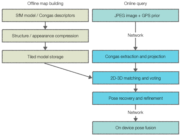
Figure 1: Overview of the complete system described in this paper, comprising of offline stages to create and compactly store the model of the environment and a real-time online query stack. The online query part on the right is split between device and server with a mobile network connection link using about 20kB per VGA resolution query image.

Fig. 1 illustrates our proposed localization approach. In the following, we briefly provide an overview over our system. We then describe each sub-component in more detail in subsequent sections.

In an offline stage, a 3D point cloud is reconstructed from a set of database images using SfM. In order to scale to large areas, we split this 3D point cloud model into subparts which cover a few street-blocks each. Each of these sub-maps is compressed by summarizing the scene structure and appearance to reduce storage, compute cost and latency for the localization queries.

The robot or mobile-phone we want to geo-localize runs a real-time visual inertial SLAM method to track the movement of the camera in a local coordinate frame. Local pose tracking provides the real-time signal for control or rendering and runs independent of the server using only on-device resources. For a subset of frames captured by the device camera, visual features are extracted and their descriptors are used to match against the descriptors of the previously built 3D point cloud. This matching step takes place on the server, where a relevant subset of the model parts are selected based on approximate location from GPS/WiFi signals. Once the models are loaded, efficient matching algorithms identify those 3D points in the model that denote the same objects as visible in the query image. The resulting 2D-3D correspondences are first filtered based on geometric constraints and subsequently used to robustly estimate the global camera pose via RANSAC (Fischler and Bolles, 1981). Given that localization has too high latency for real-time processing, we asynchronously feed the localization results into the local camera pose tracking, which continues to track the state between successful queries. The pose computed for the first frame provides the initial position and orientation of the mobile system w.r.t. to the global model. This pose thus anchors the local reference frame of the SLAM system to the global coordinates of the model. For all subsequently localized frames, the inliers to the estimated pose are integrated into the state estimator of the SLAM system to provide additional constraints (besides the features tracked by the local SLAM). These additional constraints continuously improve the alignment of the local trajectory against the global model and correct for any drift in the local tracking (Mourikis et al., 2009b; Bresson et al., 2013; Middelberg et al., 2014; Lynen et al., 2015).

4 Data and evaluation metrics used in this paper

To facilitate reading the paper and relating algorithmic description with results we interleaved the chapters with experimental evaluation. We thus first discuss the data and evaluation metrics that will be used throughout the following sections.

4.1 Model Data Acquisition

We evaluate the system on models built for the cities of Paris, Tokyo, Zurich and San Francisco to highlight parameter impact across appearance variations and scale. 3D models for each city are created from Street View collects over the last 10+ years using rigs comprising of 7 or 15 rolling-shutter cameras mounted on cars and backpacks. The camera pose and structure computation additionally leverages input from GPS, LiDAR, odometry and inertial sensors (Klingner et al., 2013) to create a global model of the environment. The model is subsequently subdivided into pieces of approximately 150x150m representing a processing unit for a given query that is convenient to store and load. We apply the model compression scheme discussed in Section 7. By enforcing a minimum of 200 of the selected landmarks to be visible in each of the cameras we obtain weak guarantees on covering all parts of the environment. A typical such model after compression consists of about 100,000 3D points and 200,000 to 500,000 visual descriptors.

4.2 Evaluation Data Acquisition and Reference Pose Computation

For each of the cities (see Table 1), we recorded evaluation sequences using consumer phones mimicking typical user behavior for augmented reality or robot navigation. These sequences are recorded from the side-walk with the phone facing downwards in walking direction or across the street. The resulting viewpoints thus exhibit substantial viewpoint differences from the views contained in the database as these were captured by cars on the street. We obtain ground truth reference poses for the evaluation sequences by automatically establishing 2D-3D matches for each frame in the evaluation sequence against the 3D model. These candidates are subsequently filtered using spatial verification taking into account the relative pose between cameras provided by SLAM (Leutenegger et al., 2014). After filtering we associate the observations from the evaluation dataset with the model landmarks. Using these constraints between local SLAM trajectory and global 3D model, we run a full-batch visual-inertial bundle adjustment to align the evaluation trajectory with the model. After alignment, the poses of the evaluation trajectory typically exhibit sub-meter/sub-degree errors wrt. the model and are thus used as reference poses for evaluation.

Table 1: The area/size of the models captured by Street View cars and the evaluation datasets used in this paper captured on foot using a mobile phone.

	Model area	Evaluation images	Evaluation sequence length
Paris	$11$ km2	$147,776$	$110$ km
Tokyo	$148$ km2	$1,688,965$	$2,036$ km
Zurich	$30$ km2	$275,587$	$186$ km
San Francisco	$34$ km2	$460,981$	$518$ km

Parameter studies were conducted using the model of Tokyo and by sampling 10% of the evaluation data ($\sim$170,000 queries) unless indicated otherwise.

4.3 Evaluation metric and approach

We use Average Precision as the main metric in this paper rather than precision/recall at a given acceptance threshold. Average precision is computed from the full precision-recall curve by taking the average of precision values at given recall $p(r)$:

$$\operatorname{AveP}=\int_{0}^{1}p(r)dr$$ (1)

We find average precision a more useful metric to compare performance given it’s independence of the chosen acceptance threshold (for instance inlier ratio of RANSAC) for localization responses. We consider a localization result to be correct if it’s position error is less than 3m and 10 degrees wrt. the reference pose.

4.4 Best performing and reference method

For each of the plots we then only replaced the module under consideration while leaving the rest of the system the same. Plots that are added throughout the text to illustrate properties of the subsystems are typically run on the best performing variant of the system (as described in detail later):

• Model with observation count compression with a budget of 500k descriptors.

• Descriptors projected to 16D and product-quantized.

• Random Grids matcher using an absolute threshold.

• Keypoint orientation and GPS prior used during matching.

• 4D voting using a maximum of 4 neighbors per query keypoint.

• p2p + gravity solver for absolute pose.

• Refinement of matches after voting.

5 Global 3D Model Creation

Depending on the deployment environment of the system, global 3D localization models are typically generated from data captured with sensors carried by cars, pedestrians, or even users of the system. We found that high quality results are most reliably obtained when using video sequences and fusing them into a single metric model of the environment (Schneider et al., 2018). In a typical Robotics setup, each such video sequence consists of thousands of images and high-frequency data from an inertial-measurement unit (IMU).

Sparse visual feature descriptors detected in the images are matched to descriptors from nearby cameras to form feature tracks. The 3D location of all tracks and the poses of the cameras are jointly estimated using metric SLAM techniques (Leutenegger et al., 2014; Mourikis et al., 2009a) to form self-consistent trajectories (including GPS, odometry and other signals if available). Subsequently, the sequences are co-registered by localizing frames from one sequence against the 3D models of other sequences and batch-filtering the results to remove outliers. We found the key ingredient for robust co-registration being metric SLAM algorithms. These allow for efficient rejection of outlier matches by comparing relative transformations from SLAM with those computed from consecutive localizations as done by Zach et al. (2010) for images in SfM. After a rigid alignment of the trajectories based on inlier matches, we run a pre-optimization of a reduced system (Johannsson et al., 2013; Nerurkar et al., 2013) with cross-trajectory constraints to eliminate low frequency errors from the trajectory. As a final step a MAP optimization (visual inertial bundle-adjustment) including inter- and intra-trajectory constraints with the following objective function is solved:

$$J(\mbf x):=\underbrace{\displaystyle\sum_{i=1}^{I}\displaystyle\sum_{j\in\mathcal{J}(i)}{\mbf e^{i,j}_{\mathrm{r}}}^{T}{\mbf W^{i,j}_{\mathrm{r}}}{\mbf e^{i,j}_{\mathrm{r}}}}_{\mathrm{visual}}+\underbrace{\displaystyle\sum_{\vphantom{j\in\mathcal{J}(i)}i=1}^{I-1}{\mbf e^{i}_{\mathrm{s}}}^{T}{\mbf W^{i}_{\mathrm{s}}}{\mbf e^{i}_{\mathrm{s}}}}_{\mathrm{inertial}}\enspace.$$ (2)

Here, $i$ denotes the camera frame index and $j$ denotes the landmark index. The set $\mathcal{J}(i)$ contains the indices of landmarks visible in the $i^{\mathrm{th}}$ frame (from the same or another trajectory). Furthermore, $\mbf W^{i,j}_{\mathrm{r}}$ represents the inverse measurement covariance of the respective visual observation, and ${\mbf W^{i}_{\mathrm{s}}}$ the inverse covariance of the $i^{\mathrm{th}}$ IMU constraint. Even for areas of the size of small cities, these optimization problems quickly exceed hundreds of thousands of camera frames with tens of millions of landmarks. In order to keep the computational time limited, we subdivide the problem into spatially disjoint sub-areas which are iteratively refined and smoothed (Guo et al., 2016; Schneider et al., 2018). See (Klingner et al., 2013) for further detail on techniques for globally optimizing a large number of trajectories to obtain models covering areas at country scale.

6 Descriptor Extraction, Selection and Projection

Due to the computational and power constraints of mobile platforms, typically cheap, yet less repeatable and discriminative visual feature descriptors are used in the SLAM frontends (Leutenegger et al., 2014; Mur-Artal and Tardós, 2017). Common choices are BRIEF (Calonder et al., ), ORB (Rublee et al., 2011), FREAK (Alahi et al., 2012) descriptors using FAST (Rosten and Drummond, 2006) or DoG (Lowe, 2004) interest points that can be computed at 30+ FPS on mobile platforms. It was shown that these descriptors typically provide sufficient discriminative power to reliably perform loop-closure, recovery and even multi-user experiences in room-scale setups (Hartmann et al., 2013).

The applicability of BRIEF, ORB, FREAK and BRISK for large scale scenes however is limited (Sun et al., 2017), in particular when the query images exhibit substantial scale and viewpoint changes. Descriptors such as SIFT (Lowe, 2004) and SURF (Bay et al., 2006) provide better performance under these conditions as well as in large scenes with strong visual aliasing. A recent analysis (Schönberger et al., 2017) showed that classical descriptors also still outperform learned variants such as LIFT (Yi et al., 2016). Learned descriptors do not yet seem to generalize well to new scenes that look sufficiently different to the training data, yet one can expect to see the situation change in the near future. Other learned descriptors like Delf (Noh et al., 2017) work well in retrieval tasks where fewer descriptors are beneficial and precise keypoint locations are not critical given that typically only approximate geometric re-ranking is performed. For localization however a high number of precisely located keypoints typically translates to a higher pose accuracy.

Trading computational cost and recognition performance is driven by the use-case and the allowed complexity of the system. Obvious options are using computationally cheap descriptors throughout the system (SLAM and global localization) or computing costlier descriptors periodically for localization queries only. As argued in our previous publication (Lynen et al., 2015), picking a single descriptor for the entire stack allows for a direct integration of localization matches into the SLAM frontend and thus reduces system-complexity compared to having two descriptor types. A separate high-quality descriptor on the other hand can significantly boost localization recall.

In the following, we focus on large scale scenes ($>20,000~{}m^{2}$) as found in indoor malls and transit stations as well as outdoor urban areas where GPS/WiFi is typically available, but has reduced accuracy. We explicitly do not focus at solving the problem of localizing globally or in an entire city since for all practical matters GPS/WiFi receivers are ubiquitous and limit the search radius. To ensure reliable performance at this scale, we compute 40 dimensional real-valued descriptors using the ‘COmpact Normalized GAbor Sampling’ (CONGAS) algorithm (Zheng et al., 2009). As in our earlier work (Lynen et al., 2015, 2017), we project the descriptors to a low-dimensional real-valued space to provide runtime improvements. For the experiments in this paper we use Principal Component Analysis (PCA) due to its simplicity and sufficient performance (Lynen et al., 2017). We reduce the descriptor to $16$ dimensions by removing the dimensions with the lowest signal-to-noise ratio to limit storage and runtime cost.

Another option to perform dimensionality reduction is to pick a projection matrix such that the $L_{2}$ distance between descriptors in the projected space matches the Likelihood Ratio Test (LRT) statistic (Bosse and Zlot, 2009; Lynen et al., 2017). The LRT is the hypothesis test that best separates matching from non-matching descriptors for a given maximum false-positive matching rate and thus allows including weak supervision when computing a projection matrix for dimensionality reduction. Other, well performing options include learned non-linear dimensionality reduction techniques as we have discussed in more detail in our earlier work (Loquercio et al., 2017).

7 The Need for Model Compression

When deploying a localization system, compactness for efficient storage as well as latency for loading and unpacking the 3D model from disk/network is a key factor. In our previous publication (Lynen et al., 2015), our proposed compression provided compactness to allow on-device localization and efficient download of the model from the server. However, also now that we want to run the localization system directly on server the same properties are key to scalability. A typical model contains around $1M$ 3D points for an area of $20,000~{}m^{2}$ which without compression would require between $500$ MB and $800$ MB of storage. Thus, covering even a medium-sized city would quickly consume several tens of TB of storage. Depending on the uncertainty of GPS, multiple sub-regions of the map need to be loaded to serve a given query and thus incur high latency.

Due to the density of data used to build the 3D models (videos or photo-collections with redundant views), only a subset of points from the initially reconstructed 3D model is necessary for successful localization. This allows us to reduce the size of the model by a process we call summarization: a combination of 3D structure subselection and appearance summarization. In addition to summarization we apply domain specific data compression to bring the storage requirements to $10$ to $15$ MB; a reduction of $>95\%$.

7.1 Structure Summarization

When capturing a scene multiple times for model construction the system can incorporate information about changes in the environment and gain robustness. At the same time however, redundant scene information leads to an increase in 3D model size.

For a real-world deployment where certain streets might have been captured hundreds of times, we thus need to solve a non-trivial subselection and compression problem: Build and maintain a model of the environment which is constant in memory size, yet capable of incorporating newly collected data over time. Early work in the Robotics community discarded entire image captures from the map (Maddern et al., 2012a, b) or formed full image descriptors (Naseer et al., 2014) used to identify novel views of the scene. Discarding entire images however ignores the fine grained information about stable environment features that are critical for robust localization. While Johns and Yang (2013) learn place dependent feature statistics to limit insertions to the database to relevant locations, the representation per location still grows unbounded.

Driven by the structure-based localization algorithm and the desire for a constant size model, we leverage subsampling and summarization techniques from the Computer Vision (Li et al., 2010; Park et al., 2013; Cao and Snavely, 2014; Camposeco et al., 2018) and Robotics (Dymczyk et al., 2015b, a; Mühlfellner et al., 2016) communities. These techniques have demonstrated that it’s possible to discard large parts of the initial 3D points with only moderate influence on the localization performance.

After such compression, only the minimal amount of data required for localization is retained, which are the 3D landmark positions together with their corresponding descriptors as well as landmark covisibility information. Since the reduction process removes the landmarks which have been observed the least or have a large estimated covariance, the overall localization performance is only marginally impacted. Performance declines more significantly only at high reduction rates (Li et al., 2010). We have also observed high compression rates in our previous work (Lynen et al., 2015; Dymczyk et al., 2015b), but interestingly not on our city scale 3D models where the map density is typically lower than in SfM models built from photo tourism collections.

Picking the optimal selection of landmarks is a set cover problem (NP-complete).

A simple heuristic implementation of this data reduction is to set an upper bound on the number of descriptors per area and assign a fraction of this total to each camera in the map; we denote this by ‘observation count’ based heuristic. For each camera one keeps landmarks that have been observed most, discarding others until the budget per camera is met. Even given this simple strategy one can achieve good compression rates while ensuring coverage across the map.

While heuristics for the selection as used by Li et al. (2010) and Dymczyk et al. (2015b) provide good results, it has been shown by Mauro et al. (2014); Havlena et al. (2013) that optimization based approaches can provide gains especially under high compression rates. These approaches target picking the most informative landmarks while ensuring that every camera must observe at least $N_{\text{thres}}$ landmarks to provide coverage across the model area. This sampling process under a coverage constraints is a set-cover problem, which was shown to be NP complete (Karp, 1972). Techniques such as Integer Linear Programming (ILP) have been used earlier by Park et al. (2013) and later by (Dymczyk et al., 2015a; Camposeco et al., 2018) to pick the optimal number of landmarks (here denoted by ‘landmark count’ based). We use the observation count of a landmark to score 3D points and then iteratively remove points from the model.

We apply our previous work (Dymczyk et al., 2015a) which extended the approach of Park et al. (2013) by augmenting the ILP problem with a term that constraints the absolute number of landmarks in the model. Using this constraint allows bounding the total memory cost to a desired memory budget. Adding this constraint to the problem however conflicts with the constraint of having a minimum number of observations for every camera and thus requires the addition of slack variables. The optimization problem selecting the best landmarks under constraints is (Dymczyk et al., 2015a):

$$\begin{split}\text{minimize}\;\mathbf{q}^{T}\mathbf{x}+\lambda\mathbf{1}^{T}\boldsymbol{\zeta}\\ \text{subject to}\;\mathbf{A}\mathbf{x}+\boldsymbol{\zeta}&\geq b\mathbf{1}\\ \sum\limits_{i=1}^{N}\mathbf{x}_{i}&=n_{\text{desired}}\\ \mathbf{x}&\in\left\{0,1\right\}^{N}\\ \boldsymbol{\zeta}&\in\{\{0\}\cup\mathbb{Z}^{+}\}^{M}.\end{split}$$ (3)

Here, $\mathbf{x}$ is a binary vector whose $i$th element is one if the $i$th point is kept in the model and zero otherwise. $\mathbf{A}$ is an $M\times N$ visibility matrix where $M$ is the number of images and $N$ the number of points in the model. $b$ denotes the minimum number of 2D-3D correspondences to keep for each camera and $\mathbf{q}$ is a weight vector which encodes the score (for instance observation count) per landmark. The same variety of scoring functions as for the greedy approach from Dymczyk et al. (2015b) can be used with ILP by incorporating their results into the linear term weight $\mathbf{q}$. While ILP based subselection is computationally expensive, we found it computationally tractable once the models are split into our 150x150m sized sub-maps and processed independently.

For each sub map we start from a full SfM model, comprising typically of 1000-2000 panoramic camera frames and up to $1M$ landmarks (before summarization). We first investigate the difference between the observation count based heuristic (which compresses the map by removing observations) and the ILP-optimization based landmark count variant (which picks the optimal number of landmarks). We create variants of the model for Tokyo with different thresholds for observation and landmark count and measure average precision over their memory footprint.

Figure 2: Different compressed variants of the Tokyo model using a heuristic observation count selection (OBS) or a ILP optimization-based landmark selection (ILP) strategy. For the values of the OBS strategy, the numbers denote the budget of descriptors, while for the ILP strategy the numbers denote the budget of landmarks. We also plot different number of sub-selected descriptors for the ILP variant as reference.

It is evident from Fig. 2 that the ILP variant outperforms the heuristic independent of the compression rates for the descriptor for the same memory budget.

7.2 Appearance Summarization

When performing map-compression based on ILP-optimization following Eq. (3), each resulting landmark is represented in the map by a set of descriptors. Typically the different descriptors do not all represent unique modes of the landmark appearance and thus add substantial redundancy to the model. Obvious choices for compressing the landmark appearance are to apply averaging or subselection as previously proposed by Sattler et al. (2017a) (mean descriptor per visual word) and Irschara et al. (2009) (k-medoid clustering to find a subset of relevant descriptors).

While the compression strategy based on landmarks provides a useful reduction, landmarks from densely collected areas have a high number of observations and thus consume much of the memory budget. While the different observations of the landmarks capture the varying modes of appearance, they often exhibit redundancy and can be equally well represented with fewer modes. Besides the structure compression by landmark selection we thus additionally perform per landmark appearance summarization to store only the relevant appearance modes per landmark. We compare standard density analysis techniques with random subselection and averaging and show their tradeoffs wrt. memory and localization performance.

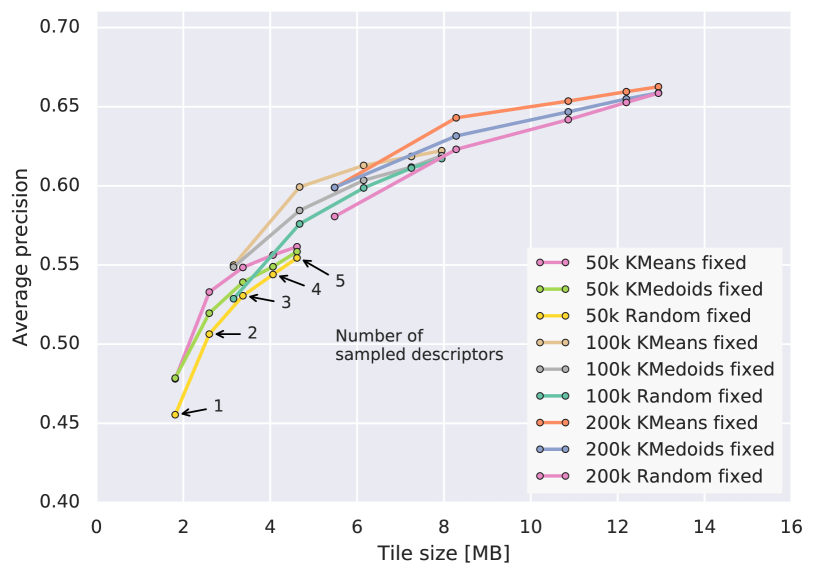
Figure 3: Combining ILP optimization based landmark selection with appearance compression using a fixed number of target descriptors per landmark. We compare performance on the Tokyo model using k-means or k-medoids centers with a random selection for different landmark budgets (denoted by the leading number).

As shown in Fig. 3, it is possible to reduce the memory footprint by around 40% at moderate performance loss. Picking the centers per landmark from k-means clustering is superior to centers from k-medoids or random selection.

Given the difference in visual saliency for points in the environment, the number of observations varies between landmarks. We found that observation count also correlates with the variance in appearance for landmark descriptors. We thus also evaluate the performance of using a fraction of the original descriptor count as the target number of descriptors to pick.

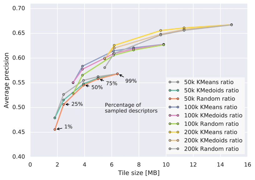
Figure 4: Combining ILP optimization based landmark selection with appearance compression using a target fraction of the original descriptors per landmark to pick. We compare performance on the Tokyo model using k-means or k-medoids centers with a random selection. The minimum number of descriptors per landmark is set to 1; where the leading number denotes the different landmark budgets.

Comparing a subset of variants using the ‘fixed count’ vs. ‘ratio’ strategies (see Fig. 5) shows a few operating points that provide beneficial memory/performance tradeoffs: for instance 200k landmarks with a summarization to 25% of the original descriptors. For the majority of operating points however the difference between the two strategies is marginal. In our system we decided to use the ILP compression picking a maximum of $200k$ landmarks per tile. For each landmark we store $25\%$ of the original descriptors picked using kmeans.

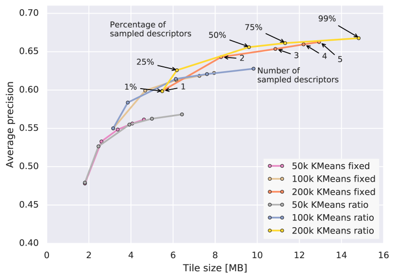
Figure 5: Comparison of performance on the Tokyo model when picking a fixed number of descriptors per landmark vs. using a ratio of the original descriptor count as a basis.

Appearance summarization also has an important effect on the end-to-end localization performance. Particularly in urban scenes local visual aliasing from repeated elements requires the retrieval of many neighbors during feature matching to achieve high recall on the 3D points. Summarizing the descriptors per landmark reduces duplicate descriptors in the index and thus increases recall during matching.

7.3 Appearance Compression

After applying landmark selection and appearance summarization, we project the selected descriptors to a lower dimensional space. The tradeoff between higher descriptor dimensions and tile size vs. average precision is shown in Fig. 6. Given diminishing returns at higher dimensions we pick 16 dimensional descriptors.

As a final data reduction step we compress the descriptors using Product Quantization (Jegou et al., 2011): The 16-dimensional descriptor space is split into $M_{\text{PQ}}$ subspaces of equal dimensionality, i.e., each descriptor is split into $M_{\text{PQ}}$ parts of length $D_{\text{PQ}}=16/M_{\text{PQ}}$. For each subspace, a visual vocabulary with $k_{\text{PQ}}$ words is learned through $k$-means clustering. These vocabularies are then used to quantize each part of a landmark descriptor individually. A descriptor is thus represented by the indices of the closest cluster center for each of its parts. This quantization significantly reduces storage requirements: E.g., when using two vocabularies ($M_{\text{PQ}}=2$) with $k_{\text{PQ}}=256$ centers each, storing a descriptor requires only 8 bytes instead of 64 bytes.

Following (Jegou et al., 2011), the squared Euclidean distance between a regular descriptor $\mathbf{d}=(\mathbf{d}_{1}~{}\cdots~{}\mathbf{d}_{M_{\text{PQ}}})$, $\mathbf{d}_{j}^{T}\in\mathbb{R}^{D_{\text{PQ}}}$, and a quantized descriptor represented by a set of indices $q=(i_{1},\dots,i_{M_{\text{PQ}}})$ is computed as

$$dist(d,q)^{2}=\sum_{j=1}^{M_{\text{PQ}}}\left(\mathbf{d}_{j}-\mathbf{c}_{j}(i_{j})\right)^{2}\enspace.$$ (4)

Here, $\mathbf{c}_{j}(i_{j})$ is the word corresponding to index $i_{j}$ in the $j^{\text{th}}$ vocabulary.

Decomposing the descriptor space such that each component has a similar variance reduces the quantization error of product quantization (Ge et al., 2014). As a result, Eq. (4) better approximates the true descriptor distance between the two original descriptors. This balancing is achieved by permuting the rows of a rotation matrix that aligns the descriptor space with its principal directions as proposed by Ge et al. (2014). Notice that this permutation does not introduce any computational overhead as the matrix is pre-computed and pre-multiplied with the projection matrix from Section 6.

With these product quantization parameters we could not measure a performance difference between the product quantized descriptors and the 16 dimensional version (see Fig. 6) which suggests further potential for compression.

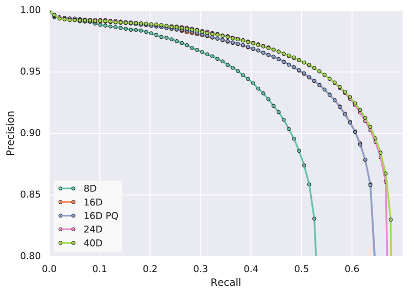
Figure 6: Comparison of different descriptor dimensions after PCA and the impact of product quantization on average precision for the Tokyo model.

8 Localization Against the Global Model

8.1 2D-3D Descriptor Matching

As briefly outlined in the introduction, localization is based on matching features from a query image against features stored in a pre-built model of the environment. The first part of localization consists of establishing 2D-3D matches between the features found in the current camera and the 3D landmarks via descriptor matching (Li et al., 2012, 2010; Sattler et al., 2017a; Svarm et al., 2014). A popular approach to accelerate the matching process is to build a kd-tree for (approximate) nearest neighbor search over the landmark descriptors (Li et al., 2012; Svarm et al., 2014). While offering good search accuracy, a kd-tree is rather slow due to backtracking and irregular memory access (Sattler et al., 2017a). Current state-of-the-art methods for efficient large-scale localization (Sattler et al., 2017a) instead use hashing and an inverted index: Given a fixed-size vocabulary, each feature descriptor from the current frame is assigned to its closest word. Exhaustive search through all landmark descriptors assigned to this word then yields the nearest neighboring landmark. This hashing approach is faster than kd-tree search and is accelerated even further through prioritization (Sattler et al., 2017a), i.e., stopping the search once a fixed number of matches has been found.

In the following we look at different methods for accelerated nearest neighbor search besides inverted indices and also revisit the decision for the inverted multi-index we took in our previous work (Lynen et al., 2015).

8.1.1 The inverted multi-index:

Obviously, larger vocabularies are desirable as fewer descriptors will be stored for every word. Yet, using a larger vocabulary implies higher assignment times and memory consumption. Both of these problems can largely be circumvented by using an inverted multi-index (Babenko and Lempitsky, 2012): Similar to product quantization, the descriptor space is split into two parts and a visual vocabulary $\mathcal{V}_{i}$ containing $N_{\text{imi}}$ words is trained for each part. The product of both vocabularies then defines a large vocabulary $\mathcal{V}=\mathcal{V}_{1}\times\mathcal{V}_{2}$ containing $N_{\text{imi}}^{2}$ words. Finding the nearest word $\omega=(\omega_{1},\omega_{2})\in\mathcal{V}$ for a descriptor $\mathbf{d}$ consists of finding the nearest neighboring words $\omega_{1}$, $\omega_{2}$ from the two smaller vocabularies $\mathcal{V}_{1}$ and $\mathcal{V}_{2}$, which we accelerated in our original work using a kd-tree (Lynen et al., 2015). Thus, using an inverted multi-index not only reduces the memory requirements but also accelerates the visual word assignments. Each landmark descriptor is assigned to its closest word from $\mathcal{V}$. For each feature that should be matched against the model, the $M$ nearest words from each vocabulary are found. From the product of these two sets of words, the feature descriptor is matched against all landmark descriptors stored in the nearest words. When using product quantization, one product quantizer is learned for each word from $\mathcal{V}_{1}$ and $\mathcal{V}_{2}$ to encode the residuals between the word and the assigned descriptors.

After landmark selection each sub-models of 150x150m contains around $500k$ to $1M$ descriptors. The inverted multi-index we used previously (Lynen et al., 2015), consists of two vocabularies with 1000 words each, yielding 1 million product words.

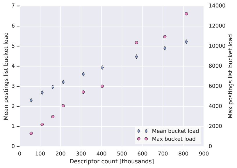
Figure 7: The bucket load in the inverted multi-index as a function of descriptor count in tiles. Both mean and max load increase rougly linear, but stay highly uneven over the buckets. Naturally these lead to long tails in the processing of hash buckets (postings lists).

Given that the vocabularies are trained independently, we found that only about $30\%$ of the product words in the vocabulary correspond to descriptors that are encountered in reality. In order to obtain high recall during matching, one typically visits multiple nearest neighbors from each sub-vocabulary. We found that between 300 and 1000 closest product words in the inverted multi-index are required for good performance. For each word we linearly process the postings list of descriptors and compute the descriptor distance. Because the k-means algorithm used to construct the vocabularies does not normalize the density of the descriptor space, commonly occuring descriptors are assigned to a small number of words. We found that in our setup the postings lists of a subset of words are very long (see Fig. 7) and cause high runtime during the query.

8.1.2 Random Grids:

To work around the shortcomings of applying the inverted multi-index in our setting, we are interested in approaches which do not require learning a vocabulary upfront and that also handle varying density in the descriptor space better. We found that the ‘Random Grids’ algorithm (Aiger et al., 2013) provides these properties and is straight forward to implement and tune. The core idea of the algorithm is to apply a random rotation and shift to the descriptor space and compute a hash-key from the transformed descriptor vector. Descriptors from both the model and query are rotated, shifted and hashed the same way. Whenever a query and database descriptor have the same hash-key, one computes the exact distance between the descriptor and conditionally stores the database index in the result list. The rotation, shift and hashing functions can be picked freely (learned) such that they provide the desired runtime/quality properties.

Differences in appearance, noise and other effects mean that hash keys for corresponding descriptors can be different and the number of hash-collisions is not high enough to lead to the desired matching recall. Therefore the random rotations, shifts and hashing is repeated $N$ times for both database and query descriptors, which means that a database descriptor is stored in $N$ different buckets. The different, independent rotations and shifts result in a higher number potentially colliding buckets between query and database and thus increase matching recall.

8.2 Evaluation of Matching Algorithms

In our previous work (Lynen et al., 2015), we compared a kd-tree (used in (Li et al., 2012; Svarm et al., 2014)), a normal inverted index (used in (Sattler et al., 2017a)), and an inverted multi-index (Babenko and Lempitsky, 2012) as techniques for establishing 2D-3D matches between query features and model points. While the inverted multi-index provided the best runtime/quality tradeoff in our previous work, we found that the random-grids index provides even higher quality than the inverted multi-index.

For the inverted multi-index used in the following experiments, we build two vocabularies containing 1,000 words each that generate a product vocabulary with 1 million words. At query time we use a kd-tree with approximation factor 0.1 (the error bound limiting backtracking) to identify the closest words from the product vocabulary.

The experiments focus on the tradeoff between quality and runtime by adjusting approximation parameters. For the inverted multi-index we vary the number of closest vocabulary words visited per descriptor. For the random-grids we vary the number of descriptors visited per grid cell.

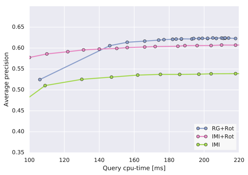
Figure 8: Comparison of the inverted multi-index (IMI) and the random grids (RG) index using the keypoint orientation (Rot) as additional signal. The underlying model is Tokyo compressed to 100k landmarks per tile using ILP compression.

While the random-grids approach outperform the inverted multi-index at query costs exceeding 150ms, the inverted multi-index was found to degrade more gracefully given the strategy we used for runtime restriction (see Fig. 8).

Given its higher quality (at moderately increased runtime cost) we leverage the random grids algorithm with 16 dimensionsional descriptors. We limit the runtime of random-grids by allowing a maximum of 100 descriptors per grid cell, which are picked at random.

8.3 Leveraging Priors During Matching:

In addition to the descriptors, we store the gravity rectified keypoint orientation as proposed by Kurz and Himane (2011). We extract gradient aligned CONGAS (Zheng et al., 2009) descriptors and then change their orientation according to the gravity direction of the camera. This method allows for faster matching (referenced as ‘GAFD-fast’ in (Kurz and Himane, 2011)) when used in the matching either as either a hard or soft filter. Hard filtering is implemented by rejecting match candidates in the postings lists (both inverted multi-index or random-grids) if their orientation doesn’t match. Soft filtering uses the (weighted) descriptor orientation as additional descriptor dimension where it becomes part of the distance calculation used to rank neighbors. See Fig. 9 for the impact of the orientation information.

Besides using GPS information to select the models to localize against, we also leverage the information as part of the nearest neighbor search to increase matching quality. In our use-case of outdoor robot and mobile-phone localization, priors from GPS/WiFi are typically available and accurate to between 5 and 50 meters. Leveraging these weighted priors allows further boosting the performance for this early stage of the pipeline as shown in Fig. 9.

For keypoint orientation and GPS prior we apply weights of $0.02$ and $0.005$ respectively, found through auto-tuning using an evaluation corpus spanning multiple cities.

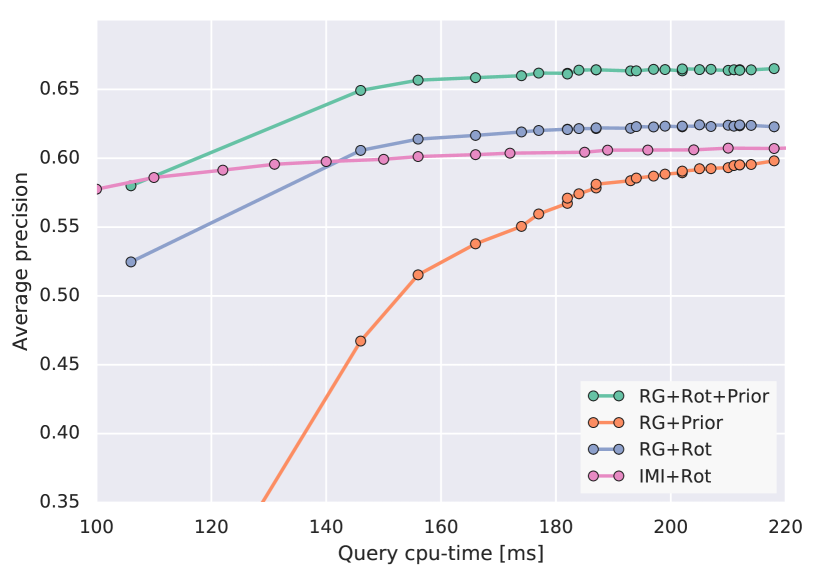
Figure 9: Comparison of the inverted multi-index (IMI) and the random grids (RG) index using the keypoint orientation (Rot) and a location prior (Prior) as additional signals. The underlying model is Tokyo compressed to 100k landmarks per tile using ILP compression.

8.4 Range Search, kNN and Thresholding:

Recall of 2D-3D matches is reduced by limited descriptor distinctiveness that arises from visual aliasing and from artifacts which occur during compression. Following previous works we thus match each keypoint from the query against $k$ neighbors from the database. Obviously increasing $k$ leads to generally higher recall on the retrieved points but also to more outliers which negatively impact later stages. Before pose recovery is performed, the ratio of outlier matches thus needs to be reduced to limit the runtime of RANSAC, which grows exponentially with the outlier ratio. A set of techniques (Sattler et al., 2017a; Zeisl et al., 2015) have been proposed to filter outlier matches. The best choice of $k$ thus depends heavily on the choice of subsequent pipeline stages. Having a too high outlier ratio decreases performance as shown in Fig. 10 with performance peaking at $k=4$ neighbors. As such, we use a set of outlier filters to reject wrong matches even for $k>1$. We complement the initial filtering based on descriptor distance with more complex, geometric and co-visibility based filters described in the next section.

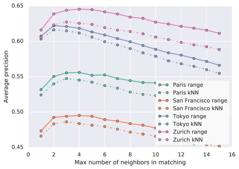
Figure 10: Localization performance as a function of the number $k$ of retrieved database points per query keypoint with (range) and without (kNN) thresholding on the descriptor distance. The underlying models are compressed using the observation count compression to 500k descriptors per tile.

We found a range search with an absolute threshold to reliably reduce outliers and improve overall performance. The exact value of the threshold depends if the descriptor is augmented with values from the keypoint orientation and prior, but appears to be globally applicable across locales as shown in Fig. 11. While filtering on descriptor distance improves performance overall, it does not significantly change the negative impact of increasing the number $k$ of retrieved matches (see Fig. 13).

Figure 11: The performance of Inverted Multi-Index and Random grids over a range of absolute threshold values and cities. The optimal threshold for Random Grids is higher since it includes error thresholds for keypoint orientation and position prior. The underlying models are compressed using the observation count compression to 500k descriptors per tile.

An alternative to filtering by absolute distance is to use the ratio test proposed by Lowe (2004). The ratio test however turns out to be non trivial to apply when matching against large models given that it’s not clear which neighbor to pick as reference: Landmarks can have a variable number of associated descriptors and several landmarks can have near identical appearance.

We would thus optimally obtain an independent reference (distractor) distribution to pick the descriptor distance from. Storing this distribution and performing the search for the reference feature however incurs additional cost. To make a fair comparison at similar runtime cost we experimented with using the vocabulary words of the inverted multi-index as reference. The distances to the closest words provide an approximation of the local descriptor space density and thus allow deriving a distance threshold for matching that takes into account the varying density in the descriptor space. This strategy is denoted as ratio test in Fig. 12.

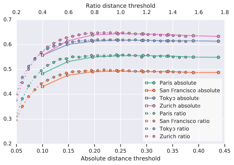
Figure 12: The performance difference between applying an absolute threshold vs. a ratio test against close words from the vocabulary of the inverted multi-index. The underlying models are compressed using the observation count compression to 500k descriptors per tile.

8.5 Co-Visibility-Based and Geometric Outlier Filtering

Often, fewer than $10\%$ of all features found in the current frame have a corresponding landmark (Sattler et al., 2017a) while others match to incorrect features. Most of these wrong matches are eliminated by a threshold on the descriptor distance as discussed in the previous section. However, some correspondences will still pass these tests, causing problems during camera pose estimation since the run-time of RANSAC increases exponentially with the outlier ratio (Fischler and Bolles, 1981). An efficient and well performing technique for outlier filtering is the “pose voting” approach by Zeisl et al. (2015) which estimates for each camera pose in the map an upper bound on the inliers using geometric constraints. The method finds the most likely camera pose by rendering surfaces that represent the geometric constraint spanned by the 2D-3D match: Each landmark’s 3D position and the angle under which is observed in the query camera span a cone in the 4D space of possible camera poses ($x$, $y$, $z$, $\kappa$). In the original algorithm, the unknowns of the camera pose are reduced to only 2D position and the rotation ($\kappa$) around the known gravity direction. While Zeisl et al. (2015) restricts voting to that 3D-space ($x$, $y$, $\kappa$) we vote directly in the pose 4-space showing that this results in better performance than the lower dimensional approximation. Since the rendered surfaces lie on a two-dimensional manifold, the rendering time in 4D space is the same as for the projected 3D space used in Zeisl et al. (2015). After rendering the surfaces for all matches, the maximima in the voting space provide a set of likely candidate poses which are further verified as described below.

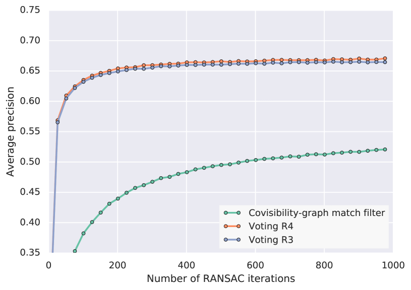
Figure 13: Evaluation of localization performance as a function of RANSAC iterations for covisibility graph based filtering and the voting approach of Zeisl et al. (2015). Note the faster convergence of the voting approach at a lower count of RANSAC iterations. The underlying models are compressed using the observation count compression to 500k descriptors per tile.

This covisibility filtering approach removes matches that do not belong to the same location in the map (Li et al., 2012; Stumm et al., 2013; Sattler et al., 2017a). The 3D model defines a undirected, bipartite visibility graph (Li et al., 2010), where the two sets of nodes correspond to the database images and the 3D landmarks in the map. A landmark node and a image node are connected if the landmark is visible in the corresponding database image. The landmarks from a given set of 2D-3D matches and their corresponding database images then form a set of connected components in this visibility graph. The covisibility filter from (Sattler et al., 2017a) simply removes all matches whose 3D point does not belong to the largest connected component.

As evaluated by Lynen et al. (2017), these algorithms however remain very sensitive to the choice of $k$ (the number of retrieved nearest neighbors per feature). Other approaches such as the vote density based technique of Lynen et al. (2017) have shown more stable performance over a wider range of values for $k$ but are computationally expensive.

We thus compare in the following voting and covisibility graph based techniques. In Sattler et al. (2017b) the covisibility graph approach outperforms the voting implementation of Zeisl et al. (2015) while for our datasets we found the opposite to be true. It seems the optimal choice is a question of dataset and implementation (see Fig. 13 and Fig. 14 for a comparison on city scale datasets).

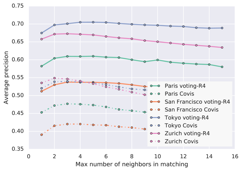
Figure 14: Performance comparison of covisibility graph filtering and voting approaches. We found that for some sequences the approaches perform very similar (as also reported by Sattler et al. (2017b)). Over a larger number of evaluation sequences and city scale models as in our setup the sparsity varies drastically over the area and a single criterion for graph expansion is difficult to pick. Here we found the performance of the covisibility filtering being degraded. The underlying models are compressed using the observation count compression to 500k descriptors per tile.

8.6 Camera Pose Estimation

After outlier removal we can estimate the camera pose given the matches. Here, we follow standard techniques: Given the knowledge of the gravity direction for both the database and the query side, we can leverage minimal solvers that exploit this additional constraint. We found that the two-point solver proposed by Sweeney et al. (2015) provides superior performance to the P3P solver of Kneip et al. (2011) as shown in Fig. 15. To improve runtime of the pose solver we use a randomized RANSAC verification approach as proposed by Matas and Chum (2004) and use the saved time to run additional iterations. The final solution is refined using PnP on all inliers (Hesch and Roumeliotis, 2011).

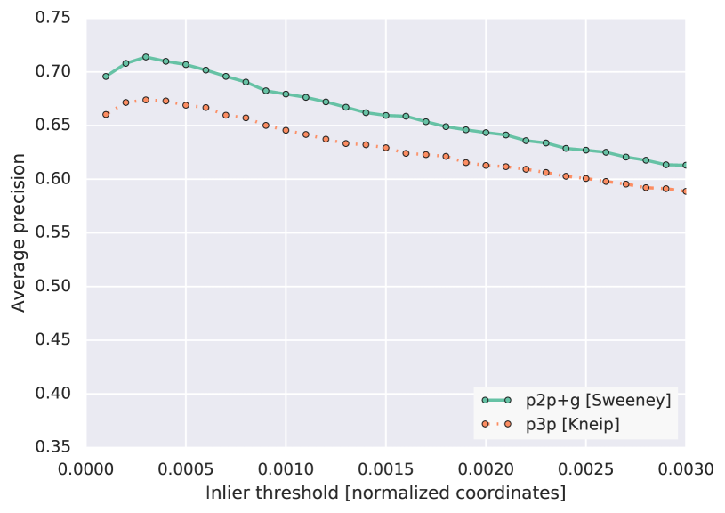
Figure 15: The absolute pose recovery performance of p2p+g (Sweeney et al., 2015) compared to P3P (Kneip et al., 2011) as a function of the inlier threshold used in RANSAC for inlier counting. The underlying model is from Zurich and compressed using the observation count compression to 500k descriptors per tile.

8.7 Pose Candidate Refinement

While increasing the number of neighbors during matching increases matching recall, the resulting increase in outliers reduces overall system performance (see Section 8.4).

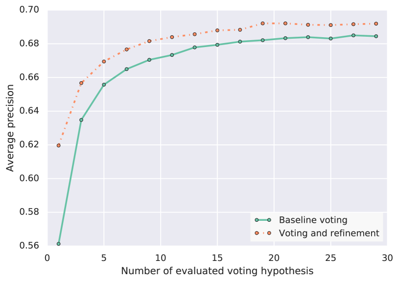
Figure 16: Comparison of our implementation of the voting approach by (Zeisl et al., 2015) with a variant using additional pose candidate refinement. Both variants use the Random Grids matcher on descriptors augmented with keypoint orientation and position prior. The underlying model is from Tokyo and compressed using the observation count compression to 500k descriptors per tile.

To recover these queries we break the localization pipeline into two hierarchical stages: First we run the matching, filtering and pose recovery steps described in the previous sections. We score maxima of the voting space based on the effective inlier count (Irschara et al., 2009) and return them as pose candidates if they are deemed reliable enough. If none of the candidates are considered good enough we run a refinement stage which breaks down the problem into smaller areas: First we identify the relevant cameras in the model using a voting scheme similar to what was proposed by Irschara et al. (2009); Gehrig et al. (2017). We want to distinguish irrelevant regions of the map which received outlier matches (at random) from those that are relevant candidates for localization. This differs from a covisibility filter since it includes a statistical model for the likelihood of random matches as a function of the descriptor density in the tile. Given the assumption that irrelevant locations receive votes randomly with probability $p$, we use the random variable $X_{i}(q_{j})$ to represent the number of matches for a keyframe $i$ given query descriptor $q_{j}$ which follows a binomial distribution:

$$X_{i}(q_{j})\sim\text{Bin}(n,p),n=N(q_{j}),p=\frac{|C_{i}|}{\sum_{k}{|C_{k}|}}\enspace,$$ (5)

where $x_{i}(q_{j})$ is the number of matches for camera $i$ given query $q_{j}$, $N_{i}:=\sum_{i}x_{i}(q_{j})$ the total number of matches for query $q_{j}$ over all cameras, $|C_{i}|$ the number of descriptors visible from camera $i$ and $\sum_{k}{|C_{k}|}$ the total number of descriptors in the model.

We expect that a location which corresponds to the true location of the query does not follow this binomial distribution. Similar to Gehrig et al. (2017) we formulate a Null-Hypothesis: For an outlier pose the number of matches $x_{i}(q_{j})$ is drawn from a binomial distribution. Every location in the map which has received more matches than expected given the random process

$$x_{i}(q_{j})>E[X_{i}(q_{j})]=N_{i}\frac{|C_{i}|}{\sum_{k}{|C_{k}|}}$$ (6)

is thus considered a relevant location to be considered for refinement. We weight this score with the pose prior from GPS and use it to rank candidates for refinement. For the top $M$ locations with high scores, we match their descriptors to the descriptors from the query and run pose recovery on the resulting 2D-3D matches.

To evaluate combining pose voting with pose refinement we vary the number of candidates $P$ evaluated during the voting step and show the effect on average precision in Fig. 16. We parallelized the pose recovery from inliers and thus limit the latency impact of increased $P$.

9 Local Pose Tracking

For any real-time application in robotics or augmented reality it is crucial to provide low-latency, low drift tracking of the camera pose relative to the environment. SLAM algorithms leveraging visual and inertial data are a common choice to provide estimates relative to a local frame of reference. By leveraging matches from the localization system one can register the local tracking against a global reference to unlock navigation and content display in the physical world.

In our system, the pose of the platform is tracked in real time using a visual-inertial sliding window estimator (implemented as an Extended Kalman Filter; EKF) with on-the-fly feature marginalization similar to the work of Mourikis et al. (2009a) with adaptations as proposed by Hesch et al. (2014). The temporally evolving state in this estimator is given by

$${\mbf x}_{E}=(^{L}{\boldsymbol{\!P}}_{I}~{}^{L}{\boldsymbol{v}}_{I}~{}{\mbf b}_{g}~{}{\mbf b}_{a})\enspace,$$ (7)

where ${}^{L}{\boldsymbol{\!P}}_{I}$ denotes the pose of the platform as the coordinate transformation of the IMU frame of reference w.r.t. the local SLAM frame of reference. The translational velocity estimate of the IMU frame w.r.t. the local SLAM frame is denoted as ${}^{L}{\boldsymbol{v}}_{I}$. ${\mbf b}_{g}$, ${\mbf b}_{a}\in\mathbb{R}^{3}$ denote the estimate of the time varying gyroscope and accelerometer bias, modeled as random walk processes driven by the zero-mean, white, Gaussian noise vectors ${\mbf n}_{bg}$ and ${\mbf n}_{ba}$.

Besides the evolving state ${\mbf x}_{E}$, the full estimated state $\hat{\mbf x}_{k}$ at time $k$ also includes the position and orientation of $N$ cameras which form the sliding window of poses (Mourikis et al., 2009a):

$$\hat{\mbf x}_{k}=(\hat{\mbf x}_{E}~{}^{L}{\boldsymbol{\!P}}_{C_{1}}~{}\cdots~{}^{L}{\boldsymbol{\!P}}_{C_{N}})\enspace.$$ (8)

Here, ${}^{L}{\boldsymbol{\!P}}_{C_{i}}$, $i=1\ldots N$, denote the estimates of the pose of the $i$th camera.

Using measurements from the IMU increases robustness and accuracy while providing a metric pose estimate. At the same time, the proper marginalization of past measurements (Dong-Si and Mourikis, 2011; Sibley et al., 2010; Nerurkar et al., 2013; Leutenegger et al., 2014) is key to obtain a smooth pose estimate. This is particularly relevant when including measurements to the global model which are often not in perfect agreement with the locally observed structure, e.g., due to moving objects during model creation or drift in the local pose estimates.

9.1 Global Updates to the Local State Estimation

In order to boot-strap the localization system, descriptors from the cameras of the local SLAM system are matched against the model as described in Section 8. Once an estimate of the pose ${}^{G}{\boldsymbol{\!P}}_{C}$ of the camera w.r.t. the global model is available, the frame of reference of the local SLAM system is aligned with the global map using the relative transformation from global model to local SLAM frame of reference ${}^{G}{\boldsymbol{\!P}}_{L}$:

$${}^{G}{\boldsymbol{\!P}}_{L} = {}^{G}{\boldsymbol{\!P}}_{C}\oplus^{C}{\boldsymbol{\!P}}_{I}\oplus^{I}{\boldsymbol{\!P}}_{L}$$ (9)

$${}^{I}{\boldsymbol{\!P}}_{L} = {}^{L}{\boldsymbol{\!P}}_{I}^{-1}.$$ (10)

Here, $\otimes$ denotes the transformation composition operator. The computed transformation ${}^{G}{\boldsymbol{\!P}}_{L}$ is subsequently integrated into the state of the SLAM system and continuously refined using 2D-3D matches from the localization system. Once the alignment of local SLAM and global map is established, we use the SLAM system’s state estimate to filter subsequent measurements using a Mahalanobis distance check. We found this to further improve the performance of the system even though most outliers are already filtered by the RANSAC step in the pose estimation during localization.

In the algorithm proposed in this paper, every associated 2D-3D match provides a measurement of the form

$${{\boldsymbol{z}}}_{i}^{(j)}=\frac{1}{{}^{C_{i}}z_{j}}\begin{bmatrix}{}^{C_{i}}x_{j}\\ {}^{C_{i}}y_{j}\end{bmatrix}+{{\boldsymbol{n}}}_{i}^{(j)}\enspace,$$ (11)

where $[^{C_{i}}x_{j}~{}^{C_{i}}y_{j}~{}^{C_{i}}z_{j}]^{T}=~{}^{C_{i}}{{\boldsymbol{p}}}_{j}$ denotes the position of the $j$th 3D point expressed in the frame of reference of camera $i$. To obtain the residual for updating the EKF, we express the expected measurement $\hat{{\boldsymbol{z}}}_{i}^{(j)}$ as a function $h$ of the state estimate $\hat{\mbf x}_{k}$ and the position of the landmark ${}^{G}{\boldsymbol{p}}_{\ell}$ expressed in the global frame of reference:

$${{\boldsymbol{r}}}_{i}^{(j)}={{\boldsymbol{z}}}_{i}^{(j)}-\hat{{\boldsymbol{z}}}_{i}^{(j)}={{\boldsymbol{z}}}_{i}^{(j)}-h(^{G}{{\boldsymbol{p}}}_{\ell},^{G}{\boldsymbol{\!P}}_{C_{i}})\enspace.$$ (12)

By linearizing this expression around the state estimate we obtain (see (Mourikis et al., 2009a), Eq. (29) for details):

$${{\boldsymbol{r}}}_{i}^{(j)}\simeq{{\boldsymbol{H}}}_{GL_{i}}^{(j)}({{\boldsymbol{x}}}_{i}-\hat{{\boldsymbol{x}}}_{i})+{{\boldsymbol{n}}}^{(j)}\enspace.$$ (13)

Here, ${{\boldsymbol{H}}}_{GL_{i}}^{(j)}$ denotes the global landmark measurement Jacobian with non-zero blocks for the pose of camera $i$.

When querying the map, it is not unusual to retrieve hundreds of matches from the image to the global map. To reduce the computational complexity of updating the estimator, all the residuals and Jacobians ${{\boldsymbol{r}}}={{\boldsymbol{H}}}({{\boldsymbol{x}}}-\hat{{\boldsymbol{x}}})+{{\boldsymbol{n}}}$ are stacked to apply measurement compression (Mourikis et al., 2009a). More specifically, we apply a QR-decomposition to ${{\boldsymbol{H}}}$:

$${{\boldsymbol{H}}}=\begin{bmatrix}{{\boldsymbol{V}}}_{1}~{}{{\boldsymbol{V}}}_{2}\end{bmatrix}\begin{bmatrix}{{\boldsymbol{T}}}_{H}\\ {{\boldsymbol{0}}}\end{bmatrix}\enspace,$$ (14)

where ${{\boldsymbol{T}}}_{H}$ is an upper triangular matrix and ${{\boldsymbol{V}}}_{1}$, ${{\boldsymbol{V}}}_{2}$ are unitary matrices with columns forming the basis for the range and the nullspace of ${{\boldsymbol{H}}}$, respectively. This operation projects the residual on the basis vectors of the range of ${{\boldsymbol{H}}}$, which means that ${{\boldsymbol{V}}}_{1}$ extracts all the information contained in the measurements. The residual from Eq. (13) can then be rewritten as

$$\begin{bmatrix}{{\boldsymbol{V}}}_{1}^{T}{{\boldsymbol{r}}}\\ {{\boldsymbol{V}}}_{2}^{T}{{\boldsymbol{r}}}\end{bmatrix}=\begin{bmatrix}{{\boldsymbol{T}}}_{H}\\ {{\boldsymbol{0}}}\end{bmatrix}({{\boldsymbol{x}}}-\hat{{\boldsymbol{x}}})+\begin{bmatrix}{{\boldsymbol{V}}}_{1}^{T}{{\boldsymbol{n}}}\\ {{\boldsymbol{V}}}_{2}^{T}{{\boldsymbol{n}}}\end{bmatrix}\enspace.$$ (15)

After discarding ${{\boldsymbol{V}}}_{2}^{T}{{\boldsymbol{r}}}$ in Eq. (15) since it only contains noise, we obtain the compressed residual formulation

$${{\boldsymbol{r}}}_{n}={{\boldsymbol{V}}}_{1}^{T}{{\boldsymbol{r}}}={{\boldsymbol{T}}}_{H}({{\boldsymbol{x}}}-\hat{{\boldsymbol{x}}})+{{\boldsymbol{n}}}_{n}\text{~{}with~{}}{{\boldsymbol{n}}}_{n}={{\boldsymbol{V}}}_{1}^{T}{{\boldsymbol{n}}}\enspace.$$ (16)

Using Givens rotations, the residual ${{\boldsymbol{r}}}_{n}$ and the upper triangular matrix ${{\boldsymbol{T}}}_{H}$ for $L$ matches can be computed efficiently in $\mathcal{O}((6N)^{2}L)$.

The MSCKF algorithm (Mourikis et al., 2009a) processes a feature track as soon as the track is broken or the entire window of cameras is spanned by the track. In our local SLAM system, these completed tracks are used to triangulate landmarks and the resulting 3D points are then used to update the estimator. When using the same visual features for frame-to-frame tracking and global localization, we can use a match between the 3D model and a feature from a single frame to identify the corresponding feature track. This information can now be used to form a constraint to the 3D model that involves all cameras that are spanned by the corresponding feature track. We found that forming a constraint which involves all key-frames which are part of the track gives a lower tracking error than performing single camera updates. To avoid double counting information, care must be taken that feature measurements are used to either formulate a constraint in the local SLAM or to the global 3D map, but not both. Given the information content of the global map, measurements to the global 3D map are preferred; where additional constraints on the updates can ensure estimator consistency (Hesch and Roumeliotis, 2012).

In order to keep memory requirements bounded, we do not store the covariance matrix for the landmarks in the map, but instead inflate the measurement noise covariance during the update assuming the landmark position errors are uncorrelated between observations. While being approximate and thus not the most accurate, the strategy allows us to keep the storage cost for a map limited. A better filtering formulation named ‘Cholesky-Schmidt-Kalman filter’ was recently proposed by DuToit et al. (2017), which allows for consistent updates and thus showed a reduction in pose error by more than $25\%$. The storage cost for this approach is only linear in the number of map landmarks, but increases the computational cost for the update by about 20x. In this paper, we thus continue to assume the map to be perfect and inflate the measurement noise of the update accordingly.

9.2 Evaluation of the Pose Fusion

Next, we evaluate the pose tracking quality achieved with our state estimator that directly includes global 2D-3D matches as EKF updates. We are interested in the position and orientation accuracy of our system, as well as the smoothness of the computed trajectories, and the time required for the state updates. We compare our system to the algorithm proposed by Middelberg et al. (2014) which performs local SLAM using a sliding window BA which optimizes only local parameters and keeps the global model fixed.

Both Middelberg et al. (2014) and Ventura et al. (2014) first compute an initial alignment using either the camera poses returned by the server or the global landmark positions. For all following frames that are sent to the server, they then optimize the alignment by including the global 2D-3D matches into the bundle adjustment of the local map. To limit the computational complexity, they perform a windowed version of SLAM based on a limited number of cameras. Cameras which are furthest away from the current pose (Middelberg et al., 2014) or oldest (Ventura et al., 2014) are discarded together with their constraints to the local and global model. Discarding (instead of properly marginalizing) measurements however has been shown to lead to suboptimal estimation performance (Dong-Si and Mourikis, 2011; Sibley et al., 2010; Leutenegger et al., 2014). The removal of constraints from the optimization also leads to discontinuities in the resulting pose estimate as the minimum of the cost function changes. To improve the performance of our reference implementation and allow a fair comparison we included IMU constraints in the bundle adjustment and use a non-linear solver that exploits the structure of the problem. Table 2 compares our method against the approach of (Middelberg et al., 2014) in which both estimators are fed with the exact same data and the same constraints to the map. For every camera frame, we evaluate the error between the estimated pose and the ground truth as the Euclidean distance between the positions and the disparity angle in orientation. As evident from the table, our EKF-based approach achieves a positional accuracy similar to the best-performing bundle adjustment approach while offering a more accurate estimate of the camera orientation. At the same time, our approach is more than one order of magnitude faster than the most efficient bundle adjustment based variant. While BA is typically run in a separate thread to avoid blocking pose tracking (Middelberg et al., 2014), the proposed EKF-based estimator is efficient enough to be directly run on each frame.

Table 2: Comparing the proposed EKF-based estimator update with sliding window bundle adjustment (BA): We report the mean time t-up required to update the estimator based on the global 2D-3D matches and the mean position $||\bar{p}_{err}||$ and orientation error $||\bar{\theta}_{err}||$ of each method (incl. std-dev.). For sliding window bundle adjustment, we experiment with using different numbers of cameras in the window (first number) and different numbers of bundle adjustment iterations (second number).

	t-up [ms]	$||\bar{p}_{err}||$ [m]	$||\bar{\theta}_{err}||$ [deg]
EKF	$2.9\pm 1.5$	$0.17\pm 0.12$	$0.32\pm 0.16$
BA-10-10	$163.0\pm 43.0$	$0.13\pm 0.15$	$0.41\pm 0.17$
BA-10-5	$138.8\pm 36.5$	$0.12\pm 0.14$	$0.58\pm 0.15$
BA-5-10	$100.3\pm 31.9$	$0.11\pm 0.13$	$0.53\pm 0.15$
BA-5-5	$77.6\pm 31.6$	$0.12\pm 0.14$	$0.57\pm 0.10$
BA-5-2	$38.6\pm 14.4$	$0.14\pm 0.16$	$0.54\pm 0.16$

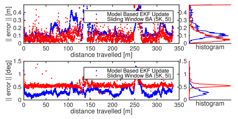
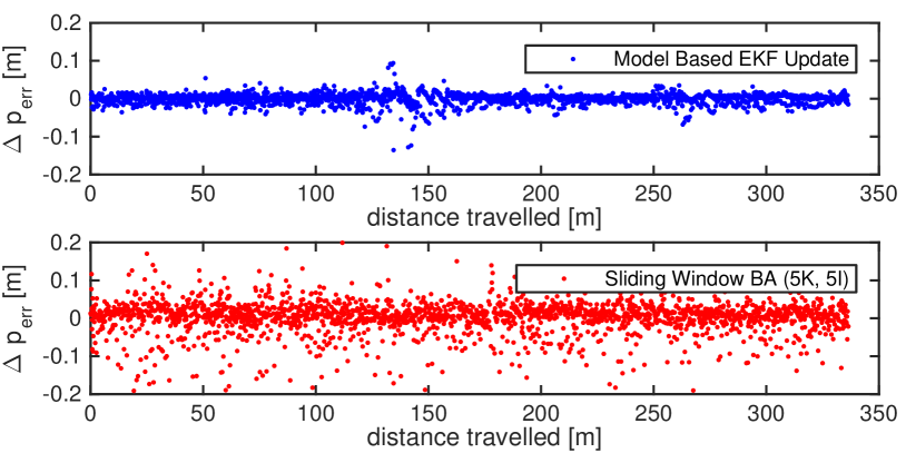
Figure 17: Compared to a sliding window bundle adjustment approach similar to (Middelberg et al., 2014), the proposed direct inclusion of the global 2D-3D matches into EKF gives significantly smoother trajectories as evident from the difference in the pose error between subsequent frames.

Fig. 17 shows that even though both approaches offer a similar mean pose accuracy, our estimator achieves a much better temporal consistency. We capture this measure by comparing the change in the error between ground truth and estimate for position and orientation. Avoiding discontinuities in pose tracking is a vital property for obstacle avoidance and robot control, where large pose jitter can cause problems when determining a path that prevents a collision. Both the runtime and accuracy metrics underline the superiority of a pose fusion approach that properly marginalizes the global constraints.

10 Conclusion

In this paper, we have presented a system for visual localization at scale. We provide details about map compression and localization algorithms that we found essential for scalable server-side deployment.

We leverage map compression techniques from the Computer Vision community and extend them with descriptor summarization to gain another 2x-4x reduction in memory footprint. With our detailed analysis of localization performance as function of map-compression algorithms we aim to provide guidance for parameter choices to the community. We also show the impact of various parameters in the localization stack including novel insights into outlier filtering strategies that allow queries with latencies in the 200ms range. Through the addition of an improved descriptor matching algorithm, position prior and a candidate refinement step we found the system to outperform other approaches when working with large scale models. We evaluate a proof-of-concept implementation of the system across four cities from three continents by querying 2.5 million images collected with smart-phone cameras. The scale of models and number of queries surpasses previous evaluations by several orders of magnitude and hopefully demonstrates the wide applicability of the parameter choices.

References

- Aiger et al. [2013] Dror Aiger, Efi Kokiopoulou, and Ehud Rivlin. Random grids: Fast approximate nearest neighbors and range searching for image search. In Proceedings of the IEEE International Conference on Computer Vision, pages 3471–3478, 2013.
- Alahi et al. [2012] Alexandre Alahi, Raphael Ortiz, and Pierre Vandergheynst. Freak: Fast retina keypoint. In Computer Vision and Pattern Recognition (CVPR), 2012 IEEE Conference on. Ieee, 2012.
- Alcantarilla et al. [2011] Pablo F Alcantarilla, Kai Ni, Luis M Bergasa, and Frank Dellaert. Visibility learning in large-scale urban environment. In 2011 IEEE International Conference on Robotics and Automation, pages 6205–6212. IEEE, 2011.
- Arandjelović et al. [2016] Relja Arandjelović, Petr Gronat, Akihito Torii, Tomas Pajdla, and Josef Sivic. NetVLAD: CNN architecture for weakly supervised place recognition. In Proceedings of the IEEE Conference on Computer Vision and Pattern Recognition (CVPR), 2016.
- Arth et al. [2009] Clemens Arth, Daniel Wagner, Manfred Klopschitz, Arnold Irschara, and Dieter Schmalstieg. Wide Area Localization on Mobile Phones. In Proceedings of the International Symposium on Mixed and Augmented Reality (ISMAR), 2009.
- Babenko and Lempitsky [2012] Artem Babenko and Victor Lempitsky. The Inverted Multi-Index. In Proceedings of the IEEE Conference on Computer Vision and Pattern Recognition (CVPR), 2012.
- Balntas et al. [2016] Vassileios Balntas, Edgar Riba, Daniel Ponsa, and Krystian Mikolajczyk. Learning local feature descriptors with triplets and shallow convolutional neural networks. In BMVC, volume 1, page 3, 2016.
- Bay et al. [2006] Herbert Bay, Tinne Tuytelaars, and Luc Van Gool. Surf: Speeded up robust features. In Proceedings of the European Conference on Computer Vision (ECCV), 2006.
- Berrio et al. [2018] Julie Stephany Berrio, James Ward, Stewart Worrall, and Eduardo Nebot. Identifying robust landmarks in feature-based maps. arXiv preprint arXiv:1809.09774, 2018.
- Bosse and Zlot [2009] Michael Bosse and Robert Zlot. Keypoint Design and Evaluation for Place Recognition in 2D Lidar Maps. Robotics and Autonomous Systems, 2009.
- Brachmann and Rother [2018] Eric Brachmann and Carsten Rother. Learning Less is More - 6D Camera Localization via 3D Surface Regression. In Proceedings of the IEEE Conference on Computer Vision and Pattern Recognition (CVPR), 2018.
- Brachmann et al. [2017] Eric Brachmann, Alexander Krull, Sebastian Nowozin, Jamie Shotton, Frank Michel, Stefan Gumhold, and Carsten Rother. DSAC - Differentiable RANSAC for Camera Localization. In Proceedings of the IEEE Conference on Computer Vision and Pattern Recognition (CVPR), 2017.
- Bresson et al. [2013] Guillaume Bresson, Romuald Aufrère, and Roland Chapuis. Making visual slam consistent with geo-referenced landmarks. In Intelligent Vehicles Symposium (IV), 2013 IEEE, pages 553–558. IEEE, 2013.
- Brown et al. [2011] Matthew Brown, Gang Hua, and Simon Winder. Discriminative learning of local image descriptors. IEEE transactions on pattern analysis and machine intelligence, 33(1):43–57, 2011.
- [15] Michael Calonder, Vincent Lepetit, Christoph Strecha, and Pascal Fua. Brief: Binary robust independent elementary features. In Computer Vision (ECCV), 2010 IEEE European Conference on, pages 778–792.
- Camposeco et al. [2017] Federico Camposeco, Torsten Sattler, Andrea Cohen, Andreas Geiger, and Marc Pollefeys. Toroidal Constraints for Two-Point Localization under High Outlier Ratios. In Proceedings of the IEEE Conference on Computer Vision and Pattern Recognition (CVPR), 2017.
- Camposeco et al. [2018] Federico Camposeco, Andrea Cohen, Marc Pollefeys, and Torsten Sattler. Hybrid scene compression for visual localization. arXiv preprint arXiv:1807.07512, 2018.
- Cao and Snavely [2013] Song Cao and Noah Snavely. Graph-based discriminative learning for location recognition. In Proceedings of the ieee conference on computer vision and pattern recognition, pages 700–707, 2013.
- Cao and Snavely [2014] Song Cao and Noah Snavely. Minimal scene descriptions from structure from motion models. In Proceedings of the IEEE Conference on Computer Vision and Pattern Recognition (CVPR), pages 461–468, 2014.
- Castle et al. [2007] Robert Oliver Castle, Darren J Gawley, Georg Klein, and David W Murray. Towards simultaneous recognition, localization and mapping for hand-held and wearable cameras. In Proceedings 2007 IEEE International Conference on Robotics and Automation, pages 4102–4107. IEEE, 2007.
- Cavallari et al. [2017] Tommaso Cavallari, Stuart Golodetz, Nicholas A Lord, Julien Valentin, Luigi Di Stefano, and Philip HS Torr. On-the-fly adaptation of regression forests for online camera relocalisation. In Proceedings of the IEEE Conference on Computer Vision and Pattern Recognition, pages 4457–4466, 2017.
- Choudhary and Narayanan [2012] Siddharth Choudhary and PJ Narayanan. Visibility probability structure from sfm datasets and applications. In European conference on computer vision, pages 130–143. Springer, 2012.
- Cummins and Newman [2011] Mark Cummins and Paul Newman. Appearance-only slam at large scale with fab-map 2.0. The International Journal of Robotics Research, 30(9):1100–1123, 2011.
- Dong-Si and Mourikis [2011] Tue-Cuong Dong-Si and Anastasios I Mourikis. Motion Tracking with Fixed-lag Smoothing: Algorithm and Consistency Analysis. In Proceedings of the IEEE International Conference on Robotics and Automation (ICRA), 2011.
- Donoser and Schmalstieg [2014] Michael Donoser and Dieter Schmalstieg. Discriminative feature-to-point matching in image-based localization. In Proceedings of the IEEE Conference on Computer Vision and Pattern Recognition, pages 516–523, 2014.
- DuToit et al. [2017] Ryan C DuToit, Joel A Hesch, Esha D Nerurkar, and Stergios I Roumeliotis. Consistent map-based 3d localization on mobile devices. In Robotics and Automation (ICRA), 2017 IEEE International Conference on, pages 6253–6260. IEEE, 2017.
- Dymczyk et al. [2015a] Marcin Dymczyk, Simon Lynen, Michael Bosse, and Roland Siegwart. Keep it brief: Scalable creation of compressed localization maps. In Intelligent Robots and Systems (IROS), 2015 IEEE/RSJ International Conference on, pages 2536–2542. IEEE, 2015a.
- Dymczyk et al. [2015b] Marcin Dymczyk, Simon Lynen, Titus Cieslewski, Michael Bosse, Roland Siegwart, and Paul Furgale. The gist of maps-summarizing experience for lifelong localization. In Robotics and Automation (ICRA), 2015 IEEE International Conference on, pages 2767–2773. IEEE, 2015b.
- Fischler and Bolles [1981] Martin A Fischler and Robert C Bolles. Random sample consensus: a paradigm for model fitting with applications to image analysis and automated cartography. Communications of the ACM, 24(6):381–395, 1981.
- Gálvez-López and Tardos [2012] Dorian Gálvez-López and Juan D Tardos. Bags of binary words for fast place recognition in image sequences. IEEE Transactions on Robotics, 28(5):1188–1197, 2012.
- Ge et al. [2014] Tiezheng Ge, Kaiming He, Qifa Ke, and Jian Sun. Optimized Product Quantization. IEEE Transactions on Pattern Analysis and Machine Intelligence (PAMI), 2014.
- Gehrig et al. [2017] Mathias Gehrig, Elena Stumm, Timo Hinzmann, and Roland Siegwart. Visual place recognition with probabilistic voting. In Robotics and Automation (ICRA), 2017 IEEE International Conference on, pages 3192–3199. IEEE, 2017.
- Guo et al. [2016] Chao X Guo, Kourosh Sartipi, Ryan C DuToit, Georgios A Georgiou, Ruipeng Li, John O’Leary, Esha D Nerurkar, Joel A Hesch, and Stergios I Roumeliotis. Large-scale cooperative 3d visual-inertial mapping in a manhattan world. In Robotics and Automation (ICRA), 2016 IEEE International Conference on, pages 1071–1078. IEEE, 2016.
- Häne et al. [2017] Christian Häne, Lionel Heng, Gim Hee Lee, Friedrich Fraundorfer, Paul Furgale, Torsten Sattler, and Marc Pollefeys. 3D Visual Perception for Self-Driving Cars using a Multi-Camera System: Calibration, Mapping, Localization, and Obstacle Detection. IMAVIS, 68:14 – 27, 2017.
- Haralick et al. [1994] Bert M Haralick, Chung-Nan Lee, Karsten Ottenberg, and Michael Nölle. Review and analysis of solutions of the three point perspective pose estimation problem. International journal of computer vision, 13(3):331–356, 1994.
- Hartmann et al. [2013] Jan Hartmann, Jan Helge Klussendorff, and Erik Maehle. A comparison of feature descriptors for visual slam. In Mobile Robots (ECMR), 2013 European Conference on, pages 56–61. IEEE, 2013.
- Havlena et al. [2013] Michal Havlena, Wilfried Hartmann, and Konrad Schindler. Optimal reduction of large image databases for location recognition. In Proceedings of the IEEE International Conference on Computer Vision Workshops, pages 676–683, 2013.
- Hesch and Roumeliotis [2011] Joel A. Hesch and Stergios I. Roumeliotis. A Direct Least-squares (DLS) solution for PnP. In Proceedings of the International Conference on Computer Vision (ICCV), 2011.
- Hesch and Roumeliotis [2012] Joel A Hesch and Stergios I Roumeliotis. Consistency analysis and improvement for single-camera localization. In Computer Vision and Pattern Recognition Workshops (CVPRW), 2012 IEEE Computer Society Conference on, pages 15–22. IEEE, 2012.
- Hesch et al. [2014] Joel A Hesch, Dimitrios G Kottas, Sean L Bowman, and Stergios I Roumeliotis. Camera-imu-based localization: Observability analysis and consistency improvement. The International Journal of Robotics Research, 33(1):182–201, 2014.
- Irschara et al. [2009] Arnold Irschara, Christopher Zach, Jan-Michael Frahm, and Horst Bischof. From Structure-from-Motion Point Clouds to Fast Location Recognition. In Proceedings of the IEEE Conference on Computer Vision and Pattern Recognition (CVPR), 2009.
- Jegou et al. [2011] Herve Jegou, Matthijs Douze, and Cordelia Schmid. Product Quantization for Nearest Neighbor Search. IEEE Transactions on Pattern Analysis and Machine Intelligence (PAMI), 33(1):117–128, 2011.
- Johannsson et al. [2013] Hordur Johannsson, Michael Kaess, Maurice Fallon, and John J Leonard. Temporally scalable visual slam using a reduced pose graph. In Robotics and Automation (ICRA), 2013 IEEE International Conference on, pages 54–61. IEEE, 2013.
- Johns and Yang [2013] Edward Johns and Guang-Zhong Yang. Feature co-occurrence maps: Appearance-based localisation throughout the day. In 2013 IEEE International Conference on Robotics and Automation, pages 3212–3218. IEEE, 2013.
- Karp [1972] Richard M Karp. Reducibility among combinatorial problems. Springer, 1972.
- Kasyanov et al. [2017] Anton Kasyanov, Francis Engelmann, Jörg Stückler, and Bastian Leibe. Keyframe-based visual-inertial online slam with relocalization. arXiv preprint arXiv:1702.02175, 2017.
- Kendall and Cipolla [2017] Alex Kendall and Roberto Cipolla. Geometric loss functions for camera pose regression with deep learning. In Proceedings of the IEEE Conference on Computer Vision and Pattern Recognition (CVPR), 2017.
- Kendall et al. [2015] Alex Kendall, Matthew Grimes, and Roberto Cipolla. Posenet: A convolutional network for real-time 6-dof camera relocalization. In Proceedings of the IEEE International Conference on Computer Vision, 2015.
- Klein and Murray [2007] Georg Klein and David Murray. Parallel tracking and mapping for small ar workspaces. In Mixed and Augmented Reality, 2007. ISMAR 2007. 6th IEEE and ACM International Symposium on, pages 225–234. IEEE, 2007.
- Klingner et al. [2013] Bryan Klingner, David Martin, and James Roseborough. Street view motion-from-structure-from-motion. In Proceedings of the IEEE International Conference on Computer Vision, pages 953–960, 2013.
- Kneip et al. [2011] Laurent Kneip, Davide Scaramuzza, and Roland Siegwart. A novel parametrization of the perspective-three-point problem for a direct computation of absolute camera position and orientation. 2011.
- Kurz and Himane [2011] Daniel Kurz and Selim Ben Himane. Inertial sensor-aligned visual feature descriptors. In Computer Vision and Pattern Recognition (CVPR), 2011 IEEE Conference on, pages 161–166. IEEE, 2011.
- Larsson et al. [2016] Viktor Larsson, Johan Fredriksson, Carl Toft, and Fredrik Kahl. Outlier Rejection for Absolute Pose Estimation with Known Orientation. In Proceedings of the British Machine Vision Conference (BMVC), 2016.
- Lepetit and Fua [2006] Vincent Lepetit and Pascal Fua. Keypoint recognition using randomized trees. IEEE transactions on pattern analysis and machine intelligence, 28(9):1465–1479, 2006.
- Leutenegger et al. [2014] Stefan Leutenegger, Simon Lynen, Michael Bosse, Roland Siegwart, and Paul Furgale. Keyframe-Based Visual-Inertial SLAM Using Nonlinear Optimization. International Journal of Robotics Research (IJRR), 2014.
- Li et al. [2010] Yunpeng Li, Noah Snavely, and Daniel P Huttenlocher. Location Recognition using Prioritized Feature Matching. In Proceedings of the European Conference on Computer Vision (ECCV), 2010.
- Li et al. [2012] Yunpeng Li, Noah Snavely, Daniel Huttenlocher, and Pascal Fua. Worldwide Pose Estimation Using 3D Point Clouds. In Proceedings of the European Conference on Computer Vision (ECCV), 2012.
- Lim et al. [2015] Hyon Lim, Sudipta N. Sinha, Michael F. Cohen, Matt Uyttendaele, and H. Jin Kim. Real-time monocular image-based 6-dof localization. International Journal of Robotics Research (IJRR), 34(4-5):476–492, 2015.
- Liu et al. [2017] Liu Liu, Hongdong Li, and Yuchao Dai. Efficient Global 2D-3D Matching for Camera Localization in a Large-Scale 3D Map. In Proceedings of the International Conference on Computer Vision (ICCV), 2017.
- Loquercio et al. [2017] Antonio Loquercio, Marcin Dymczyk, Bernhard Zeisl, Simon Lynen, Igor Gilitschenski, and Roland Siegwart. Efficient descriptor learning for large scale localization. In Robotics and Automation (ICRA), 2017 IEEE International Conference on, pages 3170–3177. IEEE, 2017.
- Lowe [2004] David G. Lowe. Distinctive image features from scale-invariant keypoints. International Journal of Computer Vision (IJCV), 2004.
- Lynen et al. [2015] Simon Lynen, Torsten Sattler, Michael Bosse, Joel Hesch, Marc Pollefeys, and Roland Siegwart. Get out of my lab: Large-scale, real-time visual-inertial localization. In Proceedings of Robotics: Science and Systems (RSS), 2015.
- Lynen et al. [2017] Simon Lynen, Michael Bosse, and Roland Siegwart. Trajectory-based place-recognition for efficient large scale localization. International Journal of Computer Vision, 124(1):49–64, 2017.
- Maddern et al. [2012a] Will Maddern, Michael Milford, and Gordon Wyeth. Towards persistent indoor appearance-based localization, mapping and navigation using cat-graph. In Intelligent Robots and Systems (IROS), 2012 IEEE/RSJ International Conference on, pages 4224–4230. IEEE, 2012a.
- Maddern et al. [2012b] William P. Maddern, Michael Milford, and Gordon Wyeth. Towards persistent localization and mapping with a continuous appearance-based topology. In Robotics: Science and Systems, 2012b.
- Matas and Chum [2004] Jiri Matas and Ondrej Chum. Randomized ransac with td, d test. Image and vision computing, 22(10):837–842, 2004.
- Mauro et al. [2014] Massimo Mauro, Hayko Riemenschneider, Alberto Signoroni, Riccardo Leonardi, and Luc Van Gool. An integer linear programming model for view selection on overlapping camera clusters. In 3D Vision (3DV), 2014 2nd International Conference on, 2014.
- Middelberg et al. [2014] Sven Middelberg, Torsten Sattler, Ole Untzelmann, and Leif Kobbelt. Scalable 6-dof localization on mobile devices. In European conference on computer vision, pages 268–283. Springer, 2014.
- Mishchuk et al. [2017] Anastasiya Mishchuk, Dmytro Mishkin, Filip Radenović, and Jiri Matas. Working hard to know your neighbor’s margins: Local descriptor learning loss. In Neural Information Processing Systems (NIPS), 2017.
- Mourikis et al. [2009a] Anastasios I Mourikis, Nikolas Trawny, Stergios I Roumeliotis, Andrew E Johnson, Adnan Ansar, and Larry Matthies. Vision-aided inertial navigation for spacecraft entry, descent, and landing. IEEE Transactions on Robotics, 25(2):264–280, 2009a.
- Mourikis et al. [2009b] Anastasios I Mourikis, Nikolas Trawny, Stergios I Roumeliotis, Andrew E Johnson, Adnan Ansar, and Larry Matthies. Vision-aided inertial navigation for spacecraft entry, descent, and landing. IEEE Transactions on Robotics, 25(2):264–280, 2009b.
- Mühlfellner et al. [2016] Peter Mühlfellner, Mathias Bürki, Michael Bosse, Wojciech Derendarz, Roland Philippsen, and Paul Furgale. Summary maps for lifelong visual localization. Journal of Field Robotics, 33(5):561–590, 2016.
- Mur-Artal and Tardós [2017] Raul Mur-Artal and Juan D Tardós. Orb-slam2: An open-source slam system for monocular, stereo, and rgb-d cameras. IEEE Transactions on Robotics, 33(5):1255–1262, 2017.
- Naseer et al. [2014] Tayyab Naseer, Luciano Spinello, Wolfram Burgard, and Cyrill Stachniss. Robust visual robot localization across seasons using network flows. In AAAI, 2014.
- Nerurkar et al. [2013] Esha D. Nerurkar, Kejian J. Wu, and Stergios I. Roumeliotis. C-klam: Constrained keyframe-based localization and mapping. In In Proc. of the Workshop on ”Multi-View Geometry in Robotics” at the Robotics: Science and Systems (RSS), 2013.
- Noh et al. [2017] Hyeonwoo Noh, Andre Araujo, Jack Sim, Tobias Weyand, and Bohyung Han. Large-scale image retrieval with attentive deep local features. In Proceedings of the IEEE Conference on Computer Vision and Pattern Recognition, pages 3456–3465, 2017.
- Park et al. [2013] Hyun Soo Park, Yu Wang, Eriko Nurvitadhi, James C Hoe, Yaser Sheikh, and Mei Chen. 3D Point Cloud Reduction Using Mixed-Integer Quadratic Programming. In IEEE Conference on Computer Vision and Pattern Recognition Workshops (CVPRW), 2013.
- Piasco et al. [2018] Nathan Piasco, Désiré Sidibé, Cédric Demonceaux, and Valérie Gouet-Brunet. A survey on visual-based localization: On the benefit of heterogeneous data. Pattern Recognition, 74:90–109, 2018.
- Radenović et al. [2016] Filip Radenović, Giorgos Tolias, and Ondrej Chum. CNN Image Retrieval Learns from BoW: Unsupervised Fine-Tuning with Hard Examples. In Proceedings of the European Conference on Computer Vision (ECCV), 2016.
- Rosten and Drummond [2006] Edward Rosten and Tom Drummond. Machine learning for high-speed corner detection. In European conference on computer vision, pages 430–443. Springer, 2006.
- Rublee et al. [2011] Ethan Rublee, Vincent Rabaud, Kurt Konolige, and Gary Bradski. Orb: An efficient alternative to sift or surf. In Computer Vision (ICCV), 2011 IEEE international conference on, pages 2564–2571. IEEE, 2011.
- Sattler et al. [2015] Torsten Sattler, Michal Havlena, Filip Radenovic, Konrad Schindler, and Marc Pollefeys. Hyperpoints and fine vocabularies for large-scale location recognition. In Proceedings of the International Conference on Computer Vision (ICCV), 12 2015.
- Sattler et al. [2016] Torsten Sattler, Michal Havlena, Konrad Schindler, and Marc Pollefeys. Large-scale location recognition and the geometric burstiness problem. In Proceedings of the IEEE Conference on Computer Vision and Pattern Recognition, pages 1582–1590, 2016.
- Sattler et al. [2017a] Torsten Sattler, Bastian Leibe, and Leif Kobbelt. Efficient & effective prioritized matching for large-scale image-based localization. IEEE Transactions on Pattern Analysis & Machine Intelligence, (9):1744–1756, 2017a.
- Sattler et al. [2017b] Torsten Sattler, Akihiko Torii, Josef Sivic, Marc Pollefeys, Hajime Taira, Masatoshi Okutomi, and Tomas Pajdla. Are Large-Scale 3D Models Really Necessary for Accurate Visual Localization? In Proceedings of the IEEE Conference on Computer Vision and Pattern Recognition (CVPR), 2017b.
- Sattler et al. [2018] Torsten Sattler, Will Maddern, Carl Toft, Akihiko Torii, Lars Hammarstrand, Erik Stenborg, Daniel Safari, Masatoshi Okutomi, Marc Pollefeys, Josef Sivic, et al. Benchmarking 6dof outdoor visual localization in changing conditions. In Proc. CVPR, volume 1, 2018.
- Schneider et al. [2018] Thomas Schneider, Marcin Dymczyk, Marius Fehr, Kevin Egger, Simon Lynen, Igor Gilitschenski, and Roland Siegwart. maplab: An open framework for research in visual-inertial mapping and localization. IEEE Robotics and Automation Letters, 3(3):1418–1425, 2018.
- Schönberger and Frahm [2016] Johannes Lutz Schönberger and Jan-Michael Frahm. Structure-from-Motion Revisited. In Proceedings of the IEEE Conference on Computer Vision and Pattern Recognition (CVPR), 2016.
- Schönberger et al. [2017] Johannes Lutz Schönberger, Hans Hardmeier, Torsten Sattler, and Marc Pollefeys. Comparative Evaluation of Hand-Crafted and Learned Local Features. In Proceedings of the IEEE Conference on Computer Vision and Pattern Recognition (CVPR), 2017.
- Schönberger et al. [2018] Johannes Lutz Schönberger, Marc Pollefeys, Andreas Geiger, and Torsten Sattler. Semantic Visual Localization. In Proceedings of the IEEE Conference on Computer Vision and Pattern Recognition (CVPR), 2018.
- Shotton et al. [2013] Jamie Shotton, Ben Glocker, Christopher Zach, Shahram Izadi, Antonio Criminisi, and Andrew Fitzgibbon. Scene coordinate regression forests for camera relocalization in rgb-d images. In Proceedings of the IEEE Conference on Computer Vision and Pattern Recognition, pages 2930–2937, 2013.
- Sibley et al. [2010] Gabe Sibley, Larry Matthies, and Gaurav Sukhatme. Sliding window filter with application to planetary landing. Journal of Field Robotics, 2010.
- Sivic and Zisserman [2003] Josef Sivic and Andrew Zisserman. Video google: A text retrieval approach to object matching in videos. In Computer Vision (ICCV), IEEE International Conference on, 2003.
- Stumm et al. [2013] Elena Stumm, Christopher Mei, and Simon Lacroix. Probabilistic Place Recognition with Covisibility Maps. In Proceedings of the IEEE/RSJ Conference on Intelligent Robots and Systems (IROS), 2013.
- Sun et al. [2017] Xun Sun, Yuanfan Xie, Pei Luo, and Liang Wang. A dataset for benchmarking image-based localization. In Proceedings of the IEEE Conference on Computer Vision and Pattern Recognition, pages 7436–7444, 2017.
- Svarm et al. [2014] Linus Svarm, Olof Enqvist, Magnus Oskarsson, and Fredrik Kahl. Accurate Localization and Pose Estimation for Large 3D Models. In Proceedings of the IEEE Conference on Computer Vision and Pattern Recognition (CVPR), 2014.
- Svärm et al. [2017] Linus Svärm, Olof Enqvist, Fredrik Kahl, and Magnus Oskarsson. City-scale localization for cameras with known vertical direction. IEEE transactions on pattern analysis and machine intelligence, 39(7):1455–1461, 2017.
- Sweeney et al. [2015] Chris Sweeney, John Flynn, Benjamin Nuernberger, Matthew Turk, and Tobias Höllerer. Efficient computation of absolute pose for gravity-aware augmented reality. In Mixed and Augmented Reality (ISMAR), 2015 IEEE International Symposium on, pages 19–24. IEEE, 2015.
- Taira et al. [2018] Hajime Taira, Masatoshi Okutomi, Torsten Sattler, Mircea Cimpoi, Marc Pollefeys, Josef Sivic, Tomas Pajdla, and Akihiko Torii. InLoc: Indoor Visual Localization with Dense Matching and View Synthesis. In Proceedings of the IEEE Conference on Computer Vision and Pattern Recognition (CVPR), 2018.
- Torii et al. [2013] Akihiko Torii, Josef Sivic, Tomas Pajdla, and Masatoshi Okutomi. Visual place recognition with repetitive structures. In Proceedings of the IEEE conference on computer vision and pattern recognition, pages 883–890, 2013.
- Torii et al. [2015] Akihiko Torii, Relja Arandjelovic, Josef Sivic, Masatoshi Okutomi, and Tomas Pajdla. 24/7 place recognition by view synthesis. In Proceedings of the IEEE Conference on Computer Vision and Pattern Recognition, pages 1808–1817, 2015.
- Tran et al. [2019] Ngoc-Trung Tran, Dang-Khoa Le Tan, Anh-Dzung Doan, Thanh-Toan Do, Tuan-Anh Bui, Mengxuan Tan, and Ngai-Man Cheung. On-device scalable image-based localization via prioritized cascade search and fast one-many ransac. IEEE Transactions on Image Processing, 28(4):1675–1690, 2019.
- Trawny and Roumeliotis [2005] Nikolas Trawny and Stergios I. Roumeliotis. Indirect Kalman Filter for 3D Attitude Estimation. University of Minnesota, Dept. of Comp. Sci. & Eng., Tech. Rep, 2, 2005.
- Valada et al. [2018] Abhinav Valada, Noha Radwan, and Wolfram Burgard. Deep Auxiliary Learning For Visual Localization And Odometry. In Proceedings of the IEEE International Conference on Robotics and Automation (ICRA), 2018.
- Valentin et al. [2015] Julien Valentin, Matthias Nießner, Jamie Shotton, Andrew Fitzgibbon, Shahram Izadi, and Philip HS Torr. Exploiting uncertainty in regression forests for accurate camera relocalization. In Proceedings of the IEEE Conference on Computer Vision and Pattern Recognition, pages 4400–4408, 2015.
- Van Opdenbosch et al. [2018] Dominik Van Opdenbosch, Tamay Aykut, Nicolas Alt, and Eckehard Steinbach. Efficient map compression for collaborative visual slam. In 2018 IEEE Winter Conference on Applications of Computer Vision (WACV), pages 992–1000. IEEE, 2018.
- Ventura et al. [2014] Jonathan Ventura, Clemens Arth, Gerhard Reitmayr, and Dieter Schmalstieg. Global Localization from Monocular SLAM on a Mobile Phone. IEEE Transactions on Visualization and Computer Graphics, 2014.
- Walch et al. [2017] Florian Walch, Caner Hazirbas, Laura Leal-Taixé, Torsten Sattler, Sebastian Hilsenbeck, and Daniel Cremers. Image-Based Localization Using LSTMs for Structured Feature Correlation. In Proceedings of the International Conference on Computer Vision (ICCV), 2017.
- Weyand et al. [2016] Tobias Weyand, Ilya Kostrikov, and James Philbin. PlaNet - Photo Geolocation with Convolutional Neural Networks. In Proceedings of the European Conference on Computer Vision (ECCV), 2016.
- Williams et al. [2007] Brian Williams, Georg Klein, and Ian Reid. Real-time slam relocalisation. 2007.
- Yi et al. [2016] Kwang Moo Yi, Eduard Trulls, Vincent Lepetit, and Pascal Fua. Lift: Learned invariant feature transform. In European Conference on Computer Vision, pages 467–483. Springer, 2016.
- Zach et al. [2010] Christopher Zach, Manfred Klopschitz, and Marc Pollefeys. Disambiguating visual relations using loop constraints. In Computer Vision and Pattern Recognition (CVPR), 2010 IEEE Conference on, pages 1426–1433. IEEE, 2010.
- Zamir and Shah [2010] Amir Roshan Zamir and Mubarak Shah. Accurate Image Localization Based on Google Maps Street View. In Proceedings of the European Conference on Computer Vision (ECCV), 2010.
- Zeisl et al. [2015] Bernhard Zeisl, Torsten Sattler, and Marc Pollefeys. Camera Pose Voting for Large-Scale Image-Based Localization. In Proceedings of the International Conference on Computer Vision (ICCV). IEEE, 2015.
- Zhang and Kosecka [2006] Wei Zhang and Jana Kosecka. Image based localization in urban environments. In null, pages 33–40. IEEE, 2006.
- Zheng et al. [2009] Yan-Tao Zheng, Ming Zhao, Yang Song, Hartwig Adam, Ulrich Buddemeier, Alessandro Bissacco, Fernando Brucher, Tat-Seng Chua, and Hartmut Neven. Tour the world: building a web-scale landmark recognition engine. In Computer vision and pattern recognition, 2009. CVPR 2009. IEEE conference on, pages 1085–1092. IEEE, 2009.