Can we constrain the dark energy equation of state parameters using configuration entropy?

Abstract

We propose a new scheme for constraining the dark energy equation of state parameter/parameters based on the study of the evolution of the configuration entropy. We analyze a set of one parameter and two parameter dynamical dark energy models and find that the derivative of the configuration entropy in all the dynamical dark energy models exhibit a minimum. The magnitude of the minimum of the entropy rate is decided by both the parametrization of the equation of state as well as the associated parameters. The location of the minimum of the entropy rate is less sensitive to the form of the parametrization but depends on the associated parameters. We determine the best fit equations for the location and magnitude of the minimum of the entropy rate in terms of the parameter/parameters of the dark energy equation of state. These relations would allow us to constrain the dark energy equation of state parameter/parameters for any given parametrization provided the evolution of the configuration entropy in the Universe is known from observations.

1 Introduction

The observations (Riess et al., 1998; Perlmutter et al., 1999) tell us that the Universe is currently undergoing an accelerated expansion which remains one of the unsolved mysteries in modern cosmology. The accelerated expansion is very often explained by invoking a hypothetical component called dark energy. The dark energy is believed to have a negative pressure which drives the cosmic acceleration despite the presence of matter in the Universe and the attractive nature of gravity.

The simplest candidate for dark energy is the cosmological constant which was originally introduced by Einstein in his General Theory of Relativity to achieve a stationary Universe. This hypothetical component has a constant energy density throughout the entire history of the Universe and has become the most dominant component only in the recent past. The origin of the cosmological constant is often linked to the vacuum energy. But unfortunately the theoretical value of the vacuum energy predicted by quantum field theory is $10^{120}$ times larger than the tiny observed value of the cosmological constant. This huge discrepancy points out that we still lack a complete theoretical understanding of the nature and origin of the cosmological constant.

There are other alternative models of dark energy like quintessence (Ratra & Peebles, 1988; Caldwell et al., 1998) and k-essence (Armendariz-Picon et al., 2001) which are based on the modifications of the matter side of the Einstein’s field equations. A number of alternatives such as $f(R)$ gravity (Buchdahl, 1970) and scalar tensor theories (Brans & Dicke, 1961) have been introduced by modifying the geometric side of the Einstein’s field equations. A detailed discussion on these dark energy models can be found in Copeland et al. (2006) and Amendola & Tsujikawa (2010). Besides these, a number of other interesting proposals originating from different physically motivated ideas include the backreaction mechanism (Buchert, 2000), effect of a large local void (Tomita, 2001; Hunt & Sarkar, 2010), entropic force (Easson et al., 2011), extra-dimension (Milton, 2003), entropy maximization (Radicella & Pavón, 2012; Pavón & Radicella, 2013), information storage in the spacetime (Padmanabhan, 2017; Padmanabhan & Padmanabhan, 2017) and configuration entropy of the Universe (Pandey, 2017, 2019).

The possibility of a dynamical dark energy (Ratra & Peebles, 1988; Caldwell et al., 1998; Armendariz-Picon et al., 2001) is a logically consistent alternative to the cosmological constant which can be constrained by observations. The phenomenological approach toward this is to introduce an equation of state (EoS) which is not constant in time. This is a generic approach and any assumption of the underlying scalar field and its dynamics is reflected in the equation of state. Many such parametrizations have been proposed in the literature. The value of the parameters in these parametrizations are constrained from different observational datasets such as SNIa, CMB, BAO.

Pandey (2017) propose that the transition of the Universe from a highly uniform and smooth state to a highly irregular and clumpy state would lead to a gradual dissipation of the configuration entropy of the mass distribution in the Universe. The evolution of the configuration entropy depends on the growth rate of structure formation in the Universe and hence can be used to distinguish different models from each other. Das & Pandey (2019) consider a set of two parameter models of dynamical dark energy and show that the evolution of the configuration entropy may help us to distinguish the different dark energy parametrizations. In a recent work, Pandey & Das (2019) show that the second derivative of the configuration entropy exhibits a prominent peak at the $\Lambda$-matter equality which can be used to constrain the values of the matter density and the cosmological constant.

In the present work, we consider a number of one parameter and two parameter models of dynamical dark energy along with the $\Lambda$CDM model and study the entropy rate in these models. We analyze the dependence of the entropy rate on the parameter/parameters associated with the dark energy equation of state and propose a new scheme to constrain them from future observations.

Figure 1: The top left and right panels respectively show $D^{2}(a)$ and $f(a)$ for different values of $\omega_{0}$ in Model 1 along with the results from the $\Lambda$CDM model. The middle left panel shows the evolution of the configuration entropy $\frac{S_{c}(a)}{S_{c}(a_{i})}$ with scale factor $a$ in Model 1. The middle right panel shows the entropy rate as a function of scale factor in Model 1. The different curves in these panels correspond to different values of $\omega_{0}$ in Model 1. The entropy rate in each of these models exhibits a minimum at a specific scale factor $a_{min}$. The value of $a_{min}$ and the magnitude of the entropy rate $[\frac{dS_{c}(a)}{da}]_{min}$ at $a_{min}$ depend on the value of the parameter $\omega_{0}$. We plot the dependence of $a_{min}$ on $\omega_{0}$ for Model 1 in the bottom left panel of this figure. The corresponding best fit line is also plotted together in the same panel. The dependence of $[\frac{dS_{c}(a)}{da}]_{min}$ on $\omega_{0}$ for Model 1 is shown in the bottom right panel. A best fit line describing this dependence is also shown together in the same panel.

Figure 2: Same as Figure 1 but for Model 2.

Figure 3: Same as Figure 1 but for Model 3.

Figure 4: Same as Figure 1 but for Model 4.

Figure 5: Same as Figure 1 but for Model 5.

2 Theory

2.1 Evolution of configuration entropy

We consider a large comoving volume $V$ and divide it into a number of identical sub-volumes $dV$. If at any instant $t$, the density $\rho(\vec{x},t)$ inside each of these sub-volumes are known then the configuration entropy of the mass distribution in the volume $V$ can be written as (Pandey, 2017),

$$S_{c}(t)=-\int\rho(\vec{x},t)\log\rho(\vec{x},t)\,dV.$$ (1)

This definition is motivated by the idea of the information entropy which was originally proposed by Shannon (1948).

Treating the mass distribution as an ideal fluid, the continuity equation in an expanding Universe is given by,

$$\frac{\partial\rho}{\partial t}+3\frac{\dot{a}}{a}\rho+\frac{1}{a}\nabla\cdot(\rho\vec{v})=0.$$ (2)

Here $a$ is the scale factor and $\vec{v}$ is the peculiar velocity of the fluid elements.

The evolution of the configuration entropy (Pandey, 2017) in volume $V$ can be obtained from Equation 2 as,

$$\frac{dS_{c}(t)}{dt}+3\frac{\dot{a}}{a}S_{c}(t)-\frac{1}{a}\int\rho(3\dot{a}+\nabla\cdot\vec{v})\,dV=0.$$ (3)

The Equation 3 can be also written as,

$$\frac{dS_{c}(a)}{da}\dot{a}+3\frac{\dot{a}}{a}S_{c}(a)-F(a)=0,$$ (4)

where,

$$F(a)=3MH(a)+\frac{1}{a}\int\rho(\vec{x},a)\nabla\cdot\vec{v}\,dV.$$ (5)

Here $H(a)$ is the Hubble parameter and $M=\int\rho(\vec{x},a)\,dV=\int\bar{\rho}(1+\delta(\vec{x},a))\,dV$ is the total mass inside the comoving volume $V$. $\bar{\rho}$ is the average density of matter within the comoving volume $V$ and $\delta(\vec{x},a)=\frac{\rho(\vec{x},a)-\bar{\rho}}{\bar{\rho}}$ is the density contrast at comoving coordinate $\vec{x}$ at time $t$. One can simplify Equation 4 further using the linear perturbation theory and get,

$$\frac{dS_{c}(a)}{da}+\frac{3}{a}(S_{c}(a)-M)+\bar{\rho}f(a)\frac{D^{2}(a)}{a}\int\delta^{2}(\vec{x})\,dV=0.$$ (6)

Here $D(a)$ is the growing mode of density perturbations and $f(a)=\frac{d\ln D}{d\ln a}$ is the dimensionless linear growth rate.

We need to solve Equation 6 to find the evolution of entropy as a function of scale factor. We first require $D(a)$ and $f(a)$ to solve Equation 6. These are cosmology dependent quantities which have to be evaluated separately for each specific model under consideration. For simplicity, we set the time independent quantities equal to $1$ in Equation 6 and solve the equation using fourth order Runge-Kutta method.

The entropy evolution is jointly determined by the the second and third term of Equation 6. The second term is decided by the initial condition and the third term is primarily determined by growth rate of structure formation. Since at very early times growth rate is negligible, entropy evolution in this period is almost completely determined by the initial condition. An analytical solution of Equation 6 ignoring the third term is given by,

$$\frac{S_{c}(a)}{S_{c}(a_{i})}=\frac{M}{S_{c}(a_{i})}+\left[1-\frac{M}{S_{c}(a_{i})}\right]\left(\frac{a_{i}}{a}\right)^{3}.$$ (7)

Here $a_{i}$ is the initial scale factor and $S_{c}(a_{i})$ is the entropy at the initial scale factor. We choose $a_{i}=10^{-3}$ throughout the analysis. The Equation 7 suggests a sudden growth in $\frac{S_{c}(a)}{S_{c}(a_{i})}$ near $a_{i}$ for $S_{c}(a_{i})<M$. Similarly a sudden drop in the value of $\frac{S_{c}(a)}{S_{c}(a_{i})}$ is expected near $a_{i}$ for $S_{c}(a_{i})>M$. These transients have nothing to do with the cosmological model concerned. The choice of the initial condition is arbitrary. We set $S_{c}(a_{i})=M$ throughout the present analysis to ignore the initial transients caused by the initial conditions.

The third term in Equation 6 becomes important only after the significant growth of structures. The goal of the present analysis is to explore the possibility of constraining the dark energy EoS parameters using the evolution of configuration entropy. The dark energy equation of state influences the growth rate of structures and hence the cosmology dependent third term in Equation 6 will be of our primary interest. The time derivative of the configuration entropy can be obtained by simply using Equation 6 or by numerical differentiation of the solution of Equation 6.

Figure 6: The top left panel shows $D^{2}(a)$ for CPL parametrization with a fixed value of $\omega_{0}$ but different values of $\omega_{1}$. The top right panel shows $f(a)$ for the same models shown in the top left panel. The bottom left panel and the bottom right panel respectively show $D^{2}(a)$ and $f(a)$ for CPL parametrization with a fixed value of $\omega_{1}$ but different values of $\omega_{0}$.

Figure 7: The top left panel shows the evolution of the configuration entropy with scale factor for CPL parametrization with a fixed value of $\omega_{0}$ but different values of $\omega_{1}$. The top right panel show the entropy rate as a function of scale factor for the results shown in the top left panel. The bottom left panel shows the evolution of the configuration entropy with scale factor for CPL parametrization with a fixed value of $\omega_{1}$ but different values of $\omega_{0}$. The respective entropy rates are shown as a function of scale factor in the bottom right panel.

Figure 8: Same as Figure 6 but for JBP parametrization.

Figure 9: Same as Figure 7 but for JBP parametrization.

Figure 10: The top left and right panels respectively show the values of $a_{min}$ and $(\frac{dS_{c}(a)}{da})_{min}$ for different combinations of $\omega_{0}$ and $\omega_{1}$ in the CPL parametrization. The middle left and right panels respectively show the respective quantities as a function of $\omega_{0}$ where we have stacked the results obtained for different $\omega_{1}$ values. The same quantities are shown as a function of $\omega_{1}$ by stacking the results obtained for different $\omega_{0}$ values in the lower left and right panels respectively. The best fit plane describing the result is also shown together in each panel.

Figure 11: Same as Figure 10 but for JBP parametrization.

2.2 Growth rate of density perturbations

To explain the presence of structure in the Universe, it is presumed that the inhomogeneities in the CMBR got amplified by the process of gravitational instability over time. The growth of these primordial density perturbations can be described by the the linear theory when the density contrast, $\delta(\vec{x},a)<<1$. In linear theory, the time evolution of the density contrast is governed by the following equation,

$$\frac{\partial^{2}\delta(\vec{x},t)}{\partial t^{2}}+2H(a)\frac{\partial\delta(\vec{x},t)}{\partial t}-\frac{3}{2}\Omega_{m0}{H_{0}}^{2}\frac{1}{a^{3}}\delta(\vec{x},t)=0.$$ (8)

Changing the variable of differentiation from $t$ to $a$ and introducing the deceleration parameter $q=-\frac{a\ddot{a}}{\dot{a}^{2}}$ we get (Linder & Jenkins, 2003),

$$\frac{\partial^{2}\delta(\vec{x},a)}{\partial a^{2}}+\left(\frac{2-q}{a}\right)\frac{\partial\delta(\vec{x},a)}{\partial a}-\frac{3}{2}\frac{1}{a^{2}}\Omega_{m0}\delta(\vec{x},a)=0.$$ (9)

The solution of Equation 8 can be written as $\delta(\vec{x},a)=d(a)\delta(\vec{x})$. Here $d(a)$ is the growing mode and $\delta(\vec{x})$ is the initial density perturbation at the comoving position $\vec{x}$. The change of variable $D(a)=\frac{\delta(\vec{x},a)}{\delta(\vec{x},a_{i})}=\frac{d(a)}{d(a_{i})}$, where $a_{i}$ is some initial scale factor, leads to (Linder & Jenkins, 2003),

$$\frac{d^{2}D(a)}{da^{2}}+\frac{3}{2a}\left[1-\frac{\omega(a)}{1+X(a)}\right]\frac{dD(a)}{da}-\frac{3}{2}\frac{X(a)}{1+X(a)}\frac{D(a)}{a^{2}}=0.$$ (10)

Here

$$X(a)=\frac{\Omega_{m0}}{1-\Omega_{m0}}e^{-3\int_{a}^{1}\omega(a^{\prime})\,d\log a^{\prime}}.$$ (11)

$\Omega_{m0}$ is the present value of the mass density parameter and $\omega(a)$ is the equation of state of dark energy. The time dependence of dark energy is encoded in $\omega(a)$. We solve Equation 10 by the fourth order Runge-Kutta method. We normalize $D(a_{0})=1$ in the $\Lambda$CDM model, where $a_{0}$ is the present value of scale factor.

To find the dimensionless linear growth rate $f(a)$, we use

$$f(a)=\left[\frac{\Omega_{m0}a^{-3}}{E^{2}(a)}\right]^{\gamma},$$ (12)

where

$$E^{2}(a)=\Omega_{m0}a^{-3}+(1-\Omega_{m0})e^{3\int_{a}^{1}[1+\omega(a^{\prime})]\,d\log a^{\prime}},$$ (13)

and (Linder, 2005)

$$\gamma=0.55+0.02\,[1+\omega(a=0.5)].$$ (14)

2.3 Different parametrizations of equation of state

Many different parametrizations of the equation of state of dynamical dark energy have been proposed in the literature which can be classified as one parameter and two parameter models depending on the number of parameter involved. We have considered a number of one parameter and two parameter models for our analysis. The parametrizations are briefly described in the following subsections. For each of the parametrizations, we use Equation 10 to find the evolution of $D(a)$ and then combine $D(a)$ and $f(a)$ to find the evolution of entropy.

2.3.1 One parameter models

We use a set of one parameter models for the dark energy equation of state provided in Yang et al. (2018). The equation of states are given below :

$$\begin{array}[]{c c c}\mbox{Model 1}&\omega(a)=\omega_{0}e^{(a-1)}&\omega_{0}=-1.367\\ \mbox{Model 2}&\omega(a)=\omega_{0}a[1-\log(a)]&\omega_{0}=-1.130\\ \mbox{Model 3}&\omega(a)=\omega_{0}ae^{(1-a)}&\omega_{0}=-1.163\\ \mbox{Model 4}&\omega(a)=\omega_{0}a[1+\sin(1-a)]&\omega_{0}=-1.244\\ \mbox{Model 5}&\omega(a)=\omega_{0}a[1+\sin^{-1}(1-a)]&\omega_{0}=-1.213\end{array}$$ (20)

All the parametrizations, except the first one approach zero as $a\rightarrow 0$. Each of these parametrizations have only one free parameter $\omega_{0}$. The values of $\omega_{0}$ provided above are the best fit values obtained by Yang et al. (2018) using CMB + BAO + JLA + CC data. We have also used these values besides the other values of $\omega_{0}$ considered in our analysis.

2.3.2 Two parameter models

(i) CPL parametrization: The equation of state in the Chevallier-Polarski-Linder parametrization (Chevallier & Polarski, 2001; Linder, 2003) is given as,

$$\omega(a)=\omega_{0}+\omega_{1}(1-a)$$ (21)

which approaches $\omega_{0}+\omega_{1}$ when $a$ approaches zero. The equation of state changes with a constant slope $-\omega_{1}$. Apart from the different possible combinations of $(\omega_{0},\omega_{1})$, we also use in our analysis the best fit values $(\omega_{0},\omega_{1})=(-1.0,-0.26)$ obtained by Tripathi et al. (2017) using SNIa + BAO + H(z) data.

(ii) JBP parametrization: In Jassal-Bagla-Padmanabhan parametrization (Jassal et al., 2005), the equation of state is parametrized as

$$\omega(a)=\omega_{0}+\omega_{1}a(1-a)$$ (22)

This parametrization approaches $\omega_{0}$ as $a$ approaches zero. The slope in this case is not constant but varies linearly with $a$. The best fit values $(\omega_{0},\omega_{1})=(-1.0,-0.38)$ obtained by Tripathi et al. (2017) using SNIa + BAO + H(z) data is also used besides the other possible combinations of $(\omega_{0},\omega_{1})$.

Table 1: This shows $a_{min}$ and $(\frac{dS_{c}(a)}{da})_{min}$ as a function of the parameter/parameters of different parametrizations. The relations are obtained by fitting the numerical results obtained for each model.

Model	$a_{min}$	$(\frac{dS_{c}(a)}{da})_{min}$
Model 1	$-0.151\omega_{0}+0.331$	$0.160\omega_{0}-0.030$
Model 2	$-0.158\omega_{0}+0.337$	$0.183\omega_{0}-0.018$
Model 3	$-0.152\omega_{0}+0.345$	$0.201\omega_{0}+0.010$
Model 4	$-0.154\omega_{0}+0.343$	$0.232\omega_{0}+0.067$
Model 5	$-0.153\omega_{0}+0.344$	$0.219\omega_{0}+0.044$
CPL	$-0.167\omega_{0}-0.018\omega_{1}+0.325$	$0.160\omega_{0}+0.048\omega_{1}-0.063$
JBP	$-0.169\omega_{0}-0.021\omega_{1}+0.321$	$0.156\omega_{0}+0.028\omega_{1}-0.069$

3 Results and Conclusions

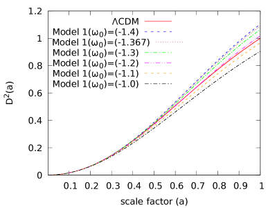
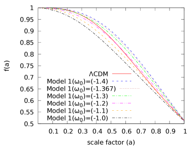
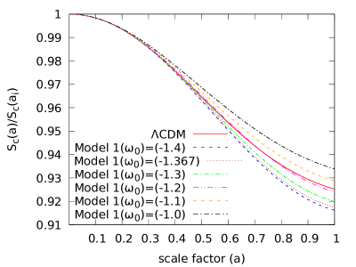
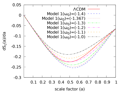
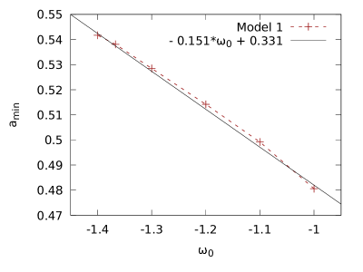
We show the square of the growing mode $D^{2}(a)$ and the dimensionless linear growth rate $f(a)$ for different values of $\omega_{0}$ in Model 1 and in the $\Lambda$CDM model in the top left and top right panel of Figure 1 respectively. In the middle left panel of Figure 1, we show the evolution of the configuration entropy $S_{c}(a)$ with scale factor for different values of $\omega_{0}$ in Model 1. The result for the $\Lambda$CDM model is also shown together with the Model 1 in the same panel. The derivative of the configuration entropy $\frac{dS_{c}(a)}{da}$ as a function of scale factor for all the cases are shown in the middle right panel of Figure 1. The configuration entropy dissipates due to the growth of inhomogeneities. We observe that the entropy dissipation rate initially increases with the increasing scale factor in all the cases. But the derivative of the entropy dissipation rate eventually changes sign at a specific scale factor. This scale factor $a_{min}$ corresponds to a minimum in the entropy rate. The entropy dissipation rate slows down after the scale factor $a_{min}$. The magnitude of the entropy rate $\frac{dS_{c}(a)}{da}$ at $a_{min}$ is directly related to the growth rate of structures in a given model and it may be noted that the models with a higher growth rate exhibit a higher entropy dissipation rate. The value of $a_{min}$ indicates the scale factor after which the dark energy plays an important role in curbing the growth of structures in the Universe. Both the value of $a_{min}$ and the entropy rate $\frac{dS_{c}(a)}{da}$ at $a_{min}$ show a systematic dependence on the parameter $\omega_{0}$ in the Model 1. We calculate the values of $a_{min}$ and $(\frac{dS_{c}(a)}{da})_{min}$ in Model 1 for different values of $\omega_{0}$. The bottom left and right panels of Figure 1 respectively show $a_{min}$ and $(\frac{dS_{c}(a)}{da})_{min}$ as a function of $\omega_{0}$ in Model 1. The best fit lines representing the numerical results (Table 1) are also plotted together in the two bottom panels of Figure 1. These results clearly indicate that the monotonic dependence of $a_{min}$ and $(\frac{dS_{c}(a)}{da})_{min}$ on $\omega_{0}$ in Model 1 can be used to constrain $\omega_{0}$ from the observational study of the evolution of the configuration entropy. Since there is only one free parameter in these models, one can either use $a_{min}$ or $(\frac{dS_{c}(a)}{da})_{min}$ to constrain the value of $\omega_{0}$ in Model 1.

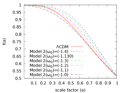
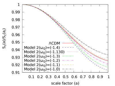
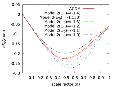
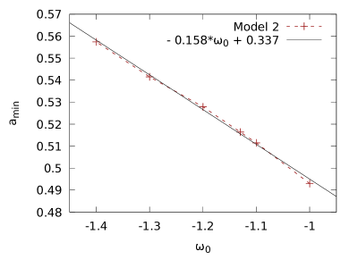
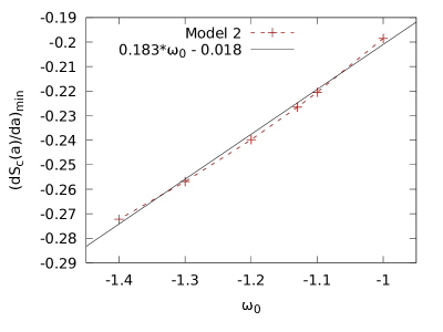
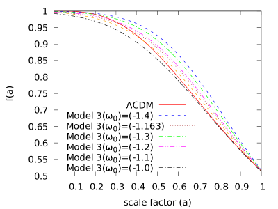
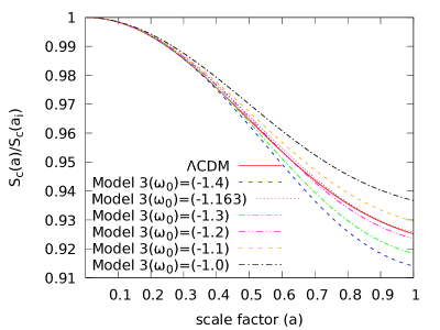
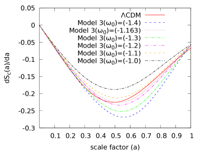
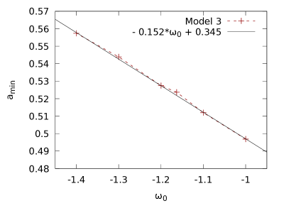
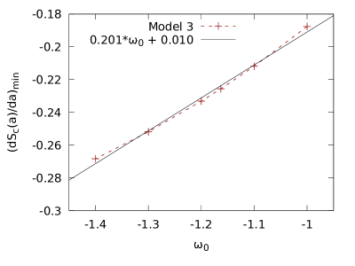
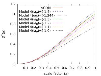
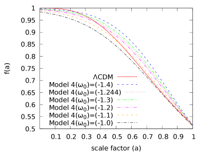
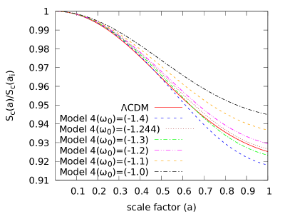
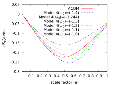
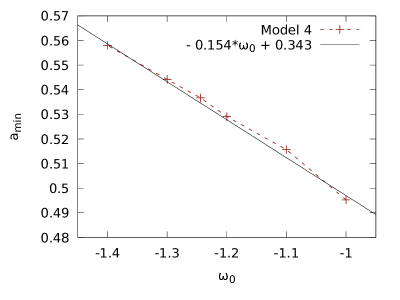
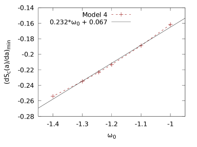
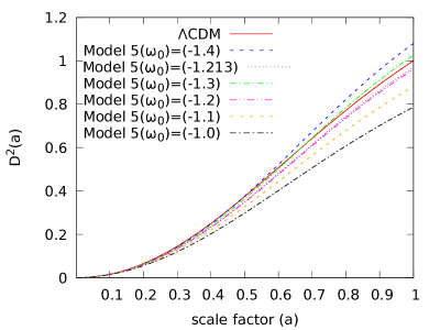
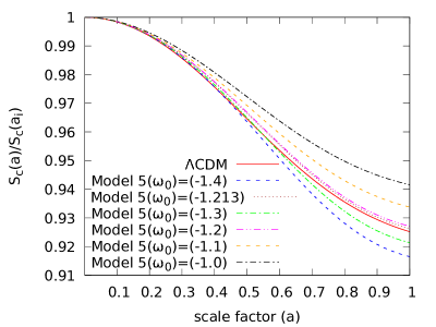
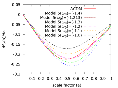
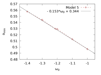
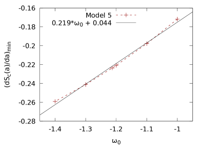
The results for Model 2, Model 3, Model 4 and Model 5 are shown in Figure 2, Figure 3, Figure 4 and Figure 5 respectively. We find that there exists a minimum in $\frac{dS_{c}(a)}{da}$ in all these models. The values of $a_{min}$ and $(\frac{dS_{c}(a)}{da})_{min}$ albeit depend on the model and the specific value of $\omega_{0}$. These results suggest that one can describe the behaviour of $a_{min}$ and $(\frac{dS_{c}(a)}{da})_{min}$ in terms of $\omega_{0}$ in each of these models. We find that both $a_{min}$ and $(\frac{dS_{c}(a)}{da})_{min}$ are linearly related to $\omega_{0}$. These linear relationships can be used to constrain the value of $\omega_{0}$ in the respective models. We find that the relationship between $a_{min}$ and $\omega_{0}$ are quite similar in all the models and hence it may not be very useful in distinguishing various one parameter models. Interestingly, the relationship between $(\frac{dS_{c}(a)}{da})_{min}$ and $\omega_{0}$ depends on the model (Table 1). This arises due to the fact that the entropy dissipation rate is sensitive to the growth rate of structures and the equation of state has a direct influence on the growth rate of structures. So this relationship may be used to discern the model as well as constrain the value of $\omega_{0}$ in that model. We also note that the location of the minimum of the entropy rate in the $\Lambda$CDM model deviates noticeably from the expectations for different values of $\omega_{0}$ in Model 3, Model 4 and Model 5. So these models can be clearly distinguished from the $\Lambda$CDM model based on such an analysis.

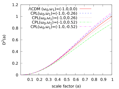
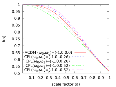
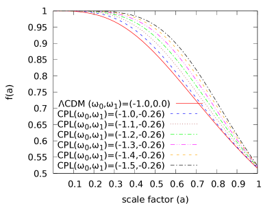
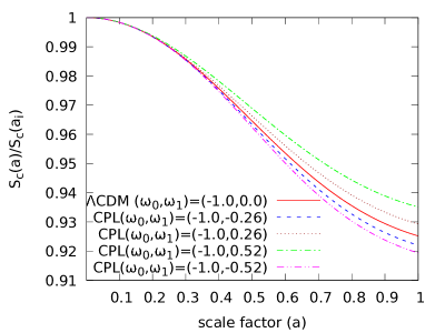
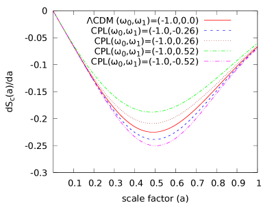
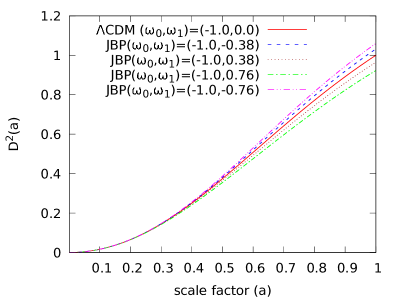
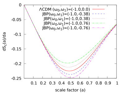
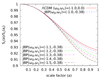
The results for the two-parameter models are shown in Figure 7 and Figure 9. In an earlier work, Das & Pandey (2019) show that the evolution of configuration entropy may help us to distinguish between different dark energy parametrizations. In the present work, we explore the possibility of constraining the parameters of a given parametrization by studying the evolution of the configuration entropy. We have considered the CPL and JBP parametrizations each of which has two parameters. We study how these parameters separately affect the evolution of the configuration entropy. The top left panel of Figure 7 shows the variation of entropy with scale factor for CPL parametrization by keeping $\omega_{0}$ fixed while varying $\omega_{1}$. We show the growing mode and the dimensionless linear growth rate for each set of EoS parameters in CPL and JBP parametrizations in Figure 6 and Figure 8 respectively. The results for the $\Lambda$CDM model is also shown together in each of the panels for comparison. The models with positive $\omega_{1}$ show less growth as compared to $\Lambda$CDM while the models with negative $\omega_{1}$ show higher growth as compared to $\Lambda$CDM. Consequently, the configuration entropy dissipates faster in the models with negative $\omega_{1}$. We show the configuration entropy rate in the top right panel of Figure 7. The derivative of the configuration entropy for the CPL parametrization also show the existence of a minimum. All the models show the minimum in entropy rate at almost the same scale factor. So the value of $a_{min}$ is less sensitive to the value of $\omega_{1}$. However, the magnitude of the entropy rate at $a_{min}$ show a relatively stronger dependence on $\omega_{1}$. This is again related to the higher growth rate in the models with negative $\omega_{1}$.

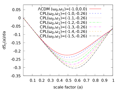
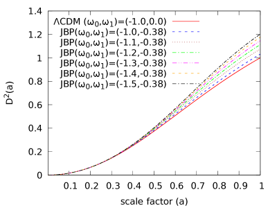
In the two bottom panels of Figure 7, we respectively show the configuration entropy and its derivative as a function of scale factor by keeping $\omega_{1}$ fixed and assuming different values for $\omega_{0}$. We find that the location of the minimum of the entropy rate systematically shifts towards higher values of scale factor with decreasing values of $\omega_{0}$. The results clearly suggest that both $a_{min}$ and $(\frac{dS_{c}(a)}{da})_{min}$ exhibit a relatively stronger dependence on $\omega_{0}$ than $\omega_{1}$.

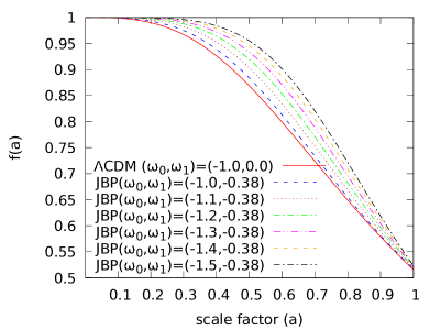
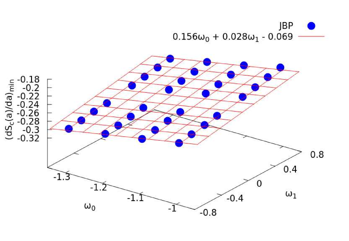
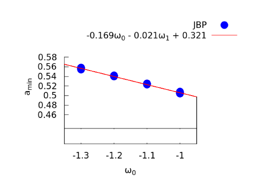
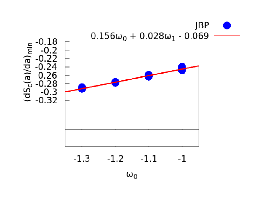
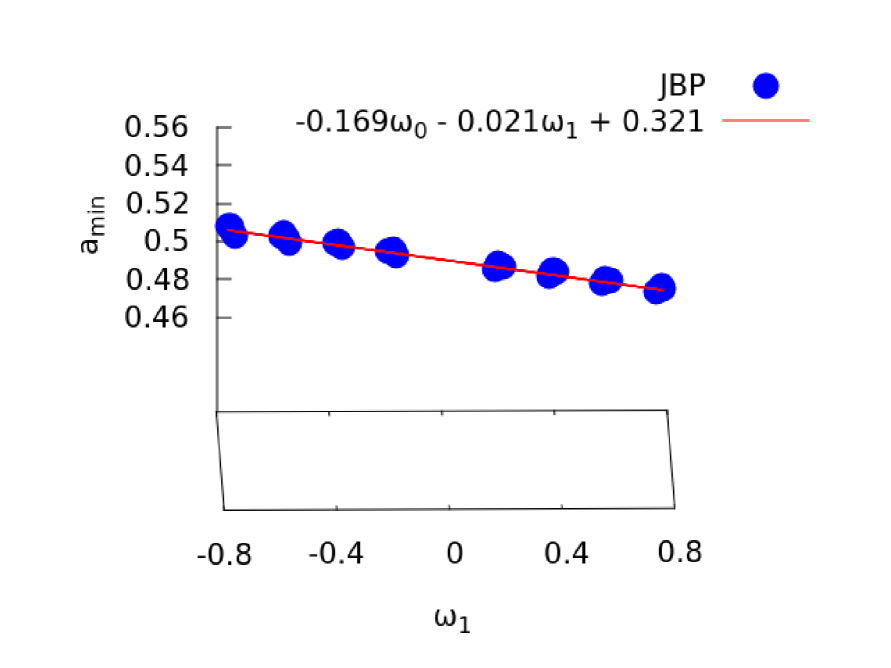
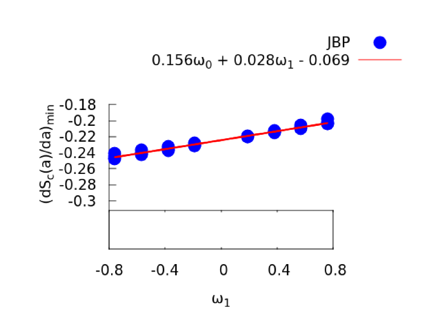
The corresponding results for the JBP parametrization are shown in different panels of Figure 9. We observe a similar trend in the behaviour of $a_{min}$ and $(\frac{dS_{c}(a)}{da})_{min}$ in case of JBP parametrization. However these two quantities show a different degree of dependence on $\omega_{0}$ and $\omega_{1}$ in the CPL and JBP parametrizations.

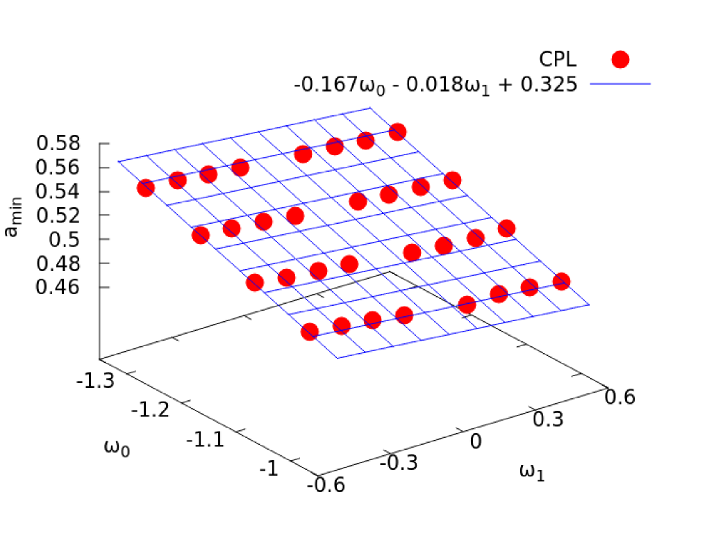
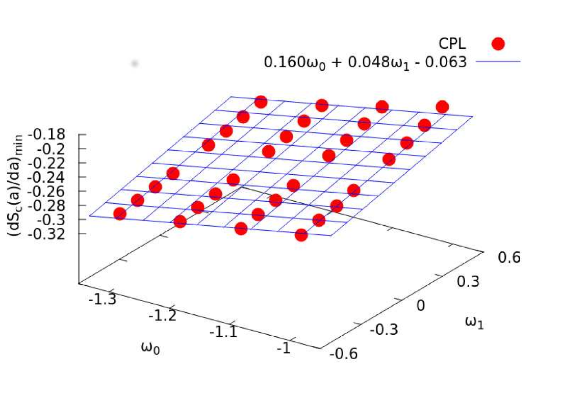
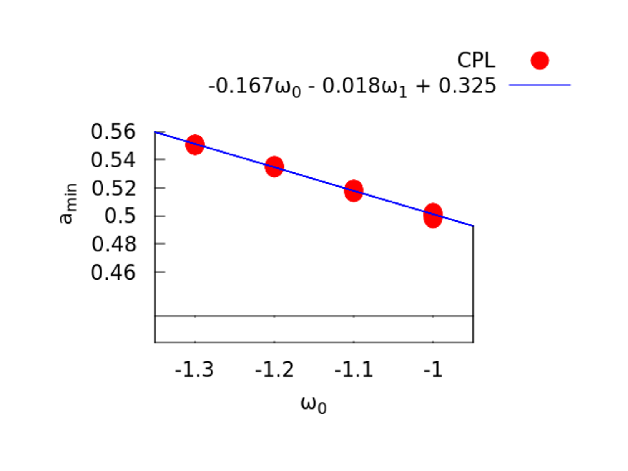
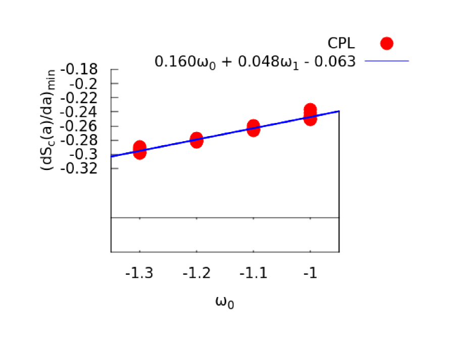
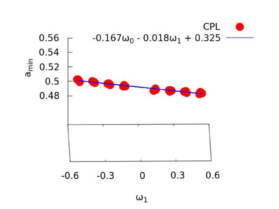
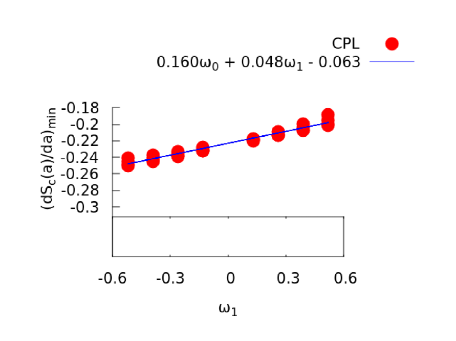
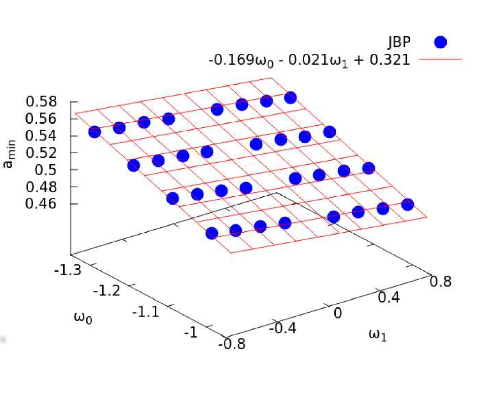
In the top left and right panels of Figure 10, we respectively plot the numerical values of $a_{min}$ and $(\frac{dS_{c}(a)}{da})_{min}$ for different combinations of $(\omega_{0},\omega_{1})$ in the CPL parametrization. We also show these results as a function of $\omega_{0}$ by stacking them for all $\omega_{1}$ in the two middle panels of Figure 10. Similarly, these quantities are shown as a function of $\omega_{1}$ by stacking the results for all $\omega_{0}$ in the two bottom panels of this figure. The respective results for the JBP parametrization are shown in the Figure 11. We also plot the best fitting surface passing through the data points in all the panels. The expressions for the best fitting planes are provided in Table 1. The results suggest that the dependence of $a_{min}$ on $\omega_{0}$ and $\omega_{1}$ are quite similar in the CPL and JBP parametrizations. We note that the dependence of $(\frac{dS_{c}(a)}{da})_{min}$ on $\omega_{0}$ and $\omega_{1}$ are somewhat different in the CPL and JBP parametrizations. The differences primarily arise due to the differences in the growth history of structures in the two parametrizations. For any given two parameter model, the two best fitting equations for $a_{min}$ and $(\frac{dS_{c}(a)}{da})_{min}$ (Table 1) can be solved together to determine $\omega_{0}$ and $\omega_{1}$ provided $a_{min}$ and $(\frac{dS_{c}(a)}{da})_{min}$ are determined from observations.

The evolution of the configuration entropy is governed by the growing mode and its derivative. So it may seem natural to directly use the growth history of large scale structures to constrain the EoS parameters (Linder & Jenkins, 2003). The possibility of using the growth rate or growth index to distinguish different cosmological models have been explored in the literature (Wang & Steinhardt, 1998; Linder, 2005; Gong et al., 2009). We can see in Figures 1-6 and Figure 8 that the growing mode and its derivative are monotonic functions of scale factor in all the models across different parametrizations considered in this work. It would be difficult to constrain the EoS parameters from these quantities given their monotonic behaviour. On the other hand, the entropy rate exhibits a distinct minimum and the location and amplitude of the minimum are sensitive to the EoS parameters and the parametrizations. The amplitude and the location of the minimum are decided by the relative dominance of the dark energy and its effect on the growth history of large scale structures. It may be noted that the configuration entropy rate depends on a specific combination of the growing mode, its derivative and the scale factor (the 3rd term in Equation 6). This specific combination is responsible for the distinct minimum observed in the derivative of the configuration entropy and we propose to use the location and amplitude of the minimum as a probe of the EoS parameters.

We would also like to point out here that the future 21 cm observations may enable us to measure the neutral Hydrogen distributions at different redshifts. This would then allow us to directly measure the configuration entropy without measuring the growing mode and its derivative. If the evolution of the HI bias (Bagla, Khandai & Datta, 2010; Guha Sarkar, et al., 2012; Padmanabhan, Choudhury & Refregier, 2015; Sarkar, Bharadwaj & Anathpindika, 2016) can be measured from these observations, the method presented in this work can be then applied to such data sets as an independent and alternative method to constrain the EoS parameters.

In this work, we propose an alternative scheme to constrain the parameters of the dynamical dark energy models by studying the time evolution of the configuration entropy in the Universe. In future, a combined analysis of the present generation redshift surveys (e.g. SDSS), the future generation surveys (e.g. Euclid) and the future 21 cm experiments (e.g. SKA) may allow us to probe the evolution of the configuration entropy in the Universe. The method presented in this work would then allow us to constrain the equation of state parameter/parameters for any given parametrization of the dark energy.

4 Acknowledgement

The authors thank an anonymous reviewer for useful comments and suggestions which helped to improve the manuscript. BP acknowledges financial support from the Science and Engineering Research Board (SERB), Department of Science & Technology (DST), Government of India through the project EMR/2015/001037. BP would also like to acknowledge IUCAA, Pune for providing support through the associateship programme.

References

- Armendariz-Picon et al. (2001) Armendariz-Picon, C., Mukhanov, V., & Steinhardt, P. J. 2001, Physical Review D, 63, 103510
- Amendola & Tsujikawa (2010) Amendola, L. & Tsujikawa, S. 2010 Dark Energy: Theory and Observation, Cambridge University Press
- Bagla, Khandai & Datta (2010) Bagla J. S., Khandai N., Datta K. K., 2010, MNRAS, 407, 567
- Brans & Dicke (1961) Brans, C. & Dicke, R. H. 1961, Physical Review, 124, 925
- Buchdahl (1970) Buchdahl, H. A. 1970, MNRAS, 150, 1
- Buchert (2000) Buchert, T. 2000, General Relativity and Gravitation, 32, 105
- Caldwell et al. (1998) Caldwell, R. R., Dave, R., & Steinhardt, P. J. 1998, Physical Review Letters, 80, 1582
- Chevallier & Polarski (2001) Chevallier, M., & Polarski, D. 2001, International Journal of Modern Physics D, 10, 213
- Copeland et al. (2006) Copeland, E. J., Sami, M., & Tsujikawa, S. 2006, International Journal of Modern Physics D, 15, 1753
- Das & Pandey (2019) Das, B., Pandey, B., 2019, MNRAS, 482, 3219
- Easson et al. (2011) Easson, D. A., Frampton, P. H., & Smoot, G. F. 2011, Physics Letters B, 696, 273
- Gong et al. (2009) Gong Y., Ishak M., Wang A., 2009, Physical Review D, 80, 023002
- Guha Sarkar, et al. (2012) Guha Sarkar T., Mitra S., Majumdar S., Choudhury T. R., 2012, MNRAS, 421, 3570
- Hunt & Sarkar (2010) Hunt, P. & Sarkar, S. 2010, MNRAS, 401, 547
- Jassal et al. (2005) Jassal, H. K., Bagla, J. S., & Padmanabhan, T. 2005, MNRAS, 356, L11
- Linder (2003) Linder, E. V. 2003, Physical Review Letters, 90, 091301
- Linder (2005) Linder, E. V. 2005, Physical Review D, 72, 043529
- Linder & Jenkins (2003) Linder, E. V., & Jenkins, A. 2003, MNRAS, 346, 573
- Milton (2003) Milton, K. A. 2003, Gravitation and Cosmology, 9, 66
- Padmanabhan, Choudhury & Refregier (2015) Padmanabhan H., Choudhury T. R., Refregier A., 2015, MNRAS, 447, 3745
- Padmanabhan (2017) Padmanabhan, T. 2017, Comptes Rendus Physique, 18, 275,
- Padmanabhan & Padmanabhan (2017) Padmanabhan, T., & Padmanabhan, H. 2017, Physics Letters B, 773, 81
- Pandey (2017) Pandey, B. 2017, MNRAS Letters, 471, L77
- Pandey (2019) Pandey, B. 2019, MNRAS Letters, 485, L73
- Pandey & Das (2019) Pandey B., Das, B. 2019, MNRAS Letters, 485, L43
- Pavón & Radicella (2013) Pavón, D., & Radicella, N. 2013, General Relativity and Gravitation, 45, 63
- Perlmutter et al. (1999) Perlmutter, S., Aldering, G., Goldhaber, G., et al. 1999, ApJ, 517, 565
- Radicella & Pavón (2012) Radicella, N., & Pavón, D. 2012, General Relativity and Gravitation, 44, 685
- Ratra & Peebles (1988) Ratra, B., & Peebles, P. J. E. 1988, Physical Review D, 37, 3406
- Riess et al. (1998) Riess, A. G., Filippenko, A. V., Challis, P., et al. 1998, AJ, 116, 1009
- Sarkar, Bharadwaj & Anathpindika (2016) Sarkar D., Bharadwaj S., Anathpindika S., 2016, MNRAS, 460, 4310
- Shannon (1948) Shannon, C. E. 1948, Bell System Technical Journal, 27, 379-423, 623-656
- Tripathi et al. (2017) Tripathi, A., Sangwan, A., & Jassal, H. K. 2017, JCAP, 6, 012
- Tomita (2001) Tomita, K. 2001, MNRAS, 326, 287
- Wang & Steinhardt (1998) Wang L., Steinhardt P. J., 1998, ApJ, 508, 483
- Yang et al. (2018) Yang W., Pan S., Di Valentino E., Saridakis E. N., Chakraborty S. 2018, Physical Review D, 99, 043543