Elastic Form Factors of Nucleon Excitations in Lattice QCD

Abstract

First principles calculations of the form factors of baryon excitations are now becoming accessible through advances in Lattice QCD techniques. In this paper, we explore the utility of the parity-expanded variational analysis (PEVA) technique in calculating the Sachs electromagnetic form factors for excitations of the proton and neutron. We study the two lowest-lying odd-parity excitations and demonstrate that at heavier quark masses, these states are dominated by behaviour consistent with constituent quark models for the $N^{*}(1535)$ and $N^{*}(1650)$, respectively. We also study the lowest-lying localised even-parity excitation, and find that its form factors are consistent with a radial excitation of the ground state nucleon. A comparison of the results from the PEVA technique with those from a conventional variational analysis exposes the necessity of the PEVA approach in baryon excited-state studies.

I Introduction

Investigating the structure of hadronic excited states is recognised as an important frontier in the field of nonperturbative QCD. At present, very little is known about how QCD composes the structure of these excitations. With regard to the excitations of the nucleon investigated herein, most of our intuition is based on models of QCD as opposed to QCD itself. The intriguing question is, how does the quantum field theory of QCD construct these states and how does this composition compare with the expectations of current models? Can something as simple as a constituent quark model capture the essence of these states? What role do meson-baryon dressings play in describing these states? Our aim is to address these most fundamental questions by examining the electromagnetic structure of nucleon excited states as observed in lattice QCD. The results are fascinating, validating quark model predictions in some cases and demanding a more important role for meson-baryon interactions in others.

A longer term goal is to confront experiment. While experimental measurements of resonance transition amplitudes have been made, it is much harder to measure elastic form factors in the resonance regime. This is because elastic form factors parameterise interactions where both the initial and final state are the same. To measure them for an (unstable) resonance, one needs to first produce that resonance, and then probe it during the extremely short time window before it decays. On the other hand, the transition form factors parameterise the transformation of one state into another. We can probe a stable target such as a ground state proton and measure how it is excited into the unstable resonance of interest through an examination of its decay products.

It has been suggested that the magnetic dipole moment of the $N^{*}(1535)$ resonance could be measured through the $\gamma p\to\gamma\eta p$ process Chiang et al. (2003) using the Crystal Barrel/TAPS detector at ELSA or Crystal Ball @ MAMI, but this measurement has yet to be realised. The difficulty of measuring such quantities experimentally provides the opportunity for Lattice QCD to lead experiment and create new knowledge.

I.1 Structure of Excited States

Here we take the first step and examine the structure of nucleon excitations as observed in the finite-volume of lattice QCD. Using local three-quark operators on the lattice, both the CSSM Mahbub et al. (2013a, b) and the Hadron Spectrum Collaboration (HSC) Edwards et al. (2013, 2011) observe two low-lying odd-parity states in the resonance regimes of the $N^{*}(1535)$ and $N^{*}(1650)$.

As these finite-volume states have good overlap with local three-quark operators, we wish to examine the extent to which these states, created in relativistic quantum field theory, resemble the quark-model states postulated to describe these resonances Chiang et al. (2003); Liu et al. (2005); Sharma et al. (2013). We anticipate the lattice-QCD states excited by such operators to be either quark-model-like states dressed by a meson cloud, similar to the ground-state nucleon, or perhaps bound meson-baryon molecular states, such as the $\Lambda(1405)$ Hall et al. (2015).

In Ref. Stokes et al. (2019), we presented a method for extracting the form factors of a baryonic state on the lattice using the parity-expanded variational analysis (PEVA) technique, and established its effectiveness for accessing the structure of the ground-state nucleon. We now use this method (as summarised in Section II) to investigate the structure of the excitations of the proton and neutron observed in the finite volume of lattice QCD.

In this paper we present a determination of the Sachs electric and magnetic form factors for three spin-$\nicefrac{{1}}{{2}}$ nucleon eigenstates on the lattice. Two of these states are negative-parity nucleon excitations, which we label ${N^{*}_{1}\!}$ (or ${p^{*}_{1}}$ for the proton excitation and ${n^{*}_{1}}$ for the neutron excitation), and ${N^{*}_{2}\!}$ (or the equivalent labels for the excited proton and neutron). The remaining eigenstate is a positive-parity excitation, and is denoted ${N^{\prime}\!}$, ${p^{\prime}}$, or ${n^{\prime}}$.

We compare the magnetic moments drawn from the negative-parity lattice-QCD results to constituent quark model predictions for the magnetic moments of the $N^{*}(1535)$ and $N^{*}(1650)$ resonances Chiang et al. (2003); Liu et al. (2005). Such quark model calculations can be extended to include effects from the pion cloud. We also compare our lattice results to two such extensions Liu et al. (2005); Sharma et al. (2013). From these comparisons, we make connections to the basis states to be considered in future Hamiltonian Effective Field Theory (HEFT) analyses Liu et al. (2016). Finally, we examine the extent to which the electromagnetic form factors of the positive-parity excitation at $\sim 1900$ MeV are consistent with a constituent-quark-model radial excitation of the ground-state nucleon.

I.2 Towards Baryon Resonance Structure

In determining resonance properties from lattice QCD calculations, one requires a comprehensive understanding of the spectrum of excited states in the finite periodic volume of the lattice. This spectrum includes all single, hybrid, and multi-particle contributions having the quantum numbers of the resonance of interest. This finite-volume spectrum composes the input into the Lüscher method Luscher (1991) or its generalisations Hall et al. (2013a); Li et al. (2019) which relate the finite-volume energy levels to infinite volume momentum-dependent scattering amplitudes. The application of these methods is a necessary step in connecting lattice QCD to the resonance properties measured in experiment.

Obtaining an accurate determination of the finite-volume nucleon spectrum is challenging. It requires an extensive collection of baryon interpolating fields and robust correlation function analysis techniques. Many collaborations have explored the nucleon spectrum excited by local single-particle operators Mahbub et al. (2012); Edwards et al. (2011, 2013); Mahbub et al. (2013a); Alexandrou et al. (2015); Kiratidis et al. (2015, 2017); Liu et al. (2017a); Lang et al. (2017). Hybrid nucleon interpolators have been investigated in Ref. Dudek and Edwards (2012) where additional states were found in the spectrum. Non-local multi-particle interpolating fields are necessary to quantify avoided level crossings and determine the lattice energy eigenstates to the level of accuracy Wilson et al. (2015) required for the implementation of the Lüscher formalism, bringing lattice-QCD results to experiment. In light of these challenges, the main approach has been to bring experimental measurements to the finite volume of the lattice Liu et al. (2017a, b); Wu et al. (2018). It is only recently that the first applications of the Lüscher formalism to the lattice-baryon spectrum have emerged Andersen et al. (2018, 2019).

The computational challenges in the baryon sector contrast the tremendous progress made within the meson sector. For example, using the formalism for connecting precision finite-volume lattice-QCD matrix-element calculations to the transition amplitudes of experiment Briceño et al. (2015a); Briceño and Hansen (2015), the resonant $\pi^{+}\gamma\to\pi^{+}\pi^{0}$ amplitude was first explored in Ref. Briceño et al. (2015b). More recently, the $\pi\pi\to\pi\gamma^{\star}$ amplitude Briceño et al. (2016), the resonant $\rho\to\pi\gamma^{\star}$ transition Briceño et al. (2016), the $\pi\gamma\to\pi\pi$ transition Alexandrou et al. (2018) and $\rho$-meson radiative decay Alexandrou et al. (2018) have been studied. In these calculations, the finite-volume lattice matrix elements are related to the physical momentum-transfer and energy-dependent scattering observables of experiment. Here a resonance appears as an enhancement as a function of the scattering energy.

A formalism for connecting the finite-volume matrix elements under investigation herein to experiment has been presented in Refs. Briceño and Hansen (2016) and Baroni et al. (2019). While our lattice-QCD formalism for matrix-element determination respects the subtleties of the finite volume, the calculations are not sufficiently precise to engage in the connection to experimental scattering observables. There, one needs the contributions of multi-particle scattering states to ensure eigenstate-projected correlation functions contain no contaminations, to quantify the exact eigenstate energies, and to include their contributions to resonances, which can be spread over several finite-volume energy eigenstates, particularly for large lattice volumes where the quantised momentum spacing becomes narrow.

The calculation of lattice matrix elements for momentum-projected meson-baryon interpolators have yet to be reported in the literature. However, their calculation for non-forward momentum transfers will be founded on the formalism presented and utilised herein.

I.3 Overview

In this paper we calculate the Sachs electric and magnetic form factors for three spin-$\nicefrac{{1}}{{2}}$ nucleon excitations observed on the finite-volume lattice. We commence with a brief summary of the parity-expanded variational analysis for matrix elements in Sec. II. There, the highlights of how the PEVA projectors alter the standard formalism is presented. Lattice QCD gauge fields, parameters and associated analysis techniques are summarised in Sec. III.

Section IV presents calculations of the electromagnetic form factors for the two low-lying negative parity excitations observed on the lattice. There, the focus is on the utility of the PEVA formalism in removing opposite-parity contaminations from the lattice correlation functions. The importance of the formalism is quantified by comparing with a conventional variational analysis where opposite-parity contaminations are not addressed through an expansion of the correlation matrix. Of particular note is a comparison of the magnetic moments drawn from the negative-parity lattice-QCD results to constituent-quark-model predictions in Sec. IV.5.

Finally, the electromagnetic structure of the first positive-parity excitation observed at $\sim 1900$ MeV in our lattice QCD calculations is presented in Sec. V. The extent to which this excitation is consistent with a constituent-quark-model radial excitation of the ground-state nucleon is of particular interest. In accord with other studies Roberts et al. (2013, 2014), we find the structure to be consistent with a radial excitation, further strengthening the case that the Roper resonance is not associated with a quark-model like state Leinweber et al. (2016); Liu et al. (2017a); Wu et al. (2018).

A summary and outline of future work is provided in the conclusions of Sec. VI.

II Parity Expanded Variational Analysis

The process of extracting finite-momentum matrix elements of baryonic excited states via the PEVA technique is presented in full in Ref Stokes et al. (2019). We provide here a brief summary of this process to introduce the notation and concepts necessary to present our results.

The idea of using operator overlaps to project onto excited states Dudek et al. (2009); Owen et al. (2015); Shultz et al. (2015) and separate opposite parities Thomas et al. (2012); Padmanath et al. (2019) has also been considered in the meson sector. In this case, matrix elements can be extracted using standard techniques Dudek et al. (2009); Owen et al. (2015); Shultz et al. (2015) as the intricacies of parity mixing within the spinor components of the correlator are absent. In the baryon sector, one must take the PEVA projectors into account in identifying the appropriate Dirac-index combinations required to isolate the covariant vertex functions and associated Sachs form factors.

We begin with a basis of $n$ conventional spin-$\nicefrac{{1}}{{2}}$ operators $\left\{{\chi_{{i}}(x)}\right\}$ that couple to the states of interest. Adopting the Pauli representation of the gamma matrices, we introduce the PEVA projector Stokes et al. (2015) ${\Gamma_{\!{\pm\bm{p}}}}\equiv\frac{1}{4}\left(\mathbb{I}+{{\gamma^{{4}}}}\right)\left(\mathbb{I}\pm i{{\gamma^{{5}}}}{{\gamma^{{k}}}}{{\smash{\widehat{\bm{p}}}\;\!\vphantom{p}}^{{k}}}\right)$, and construct a set of basis operators

$${\chi_{{\pm\bm{p}}\,{i}}(x)} \equiv{\Gamma_{\!{\pm\bm{p}}}}\,{\chi_{{i}}(x)}\,,$$ (1a)

$${\chi_{{\pm\bm{p}}\,{i^{\prime}}}(x)} \equiv\pm{\Gamma_{\!{\pm\bm{p}}}}\,{\gamma^{{5}}}{}\,{\chi_{{i}}(x)}\,.$$ (1b)

We note that we use a Euclidean metric ${\delta^{{\mu}{\nu}}}{}$, and hence there is no need to distinguish between contravariant and covariant indices.

We then seek an optimised set of operators ${\phi^{{\alpha}\,{}}_{{\pm\bm{p}}}(x)}$ that each couple strongly to a single energy eigenstate ${\alpha}$. These optimised operators are constructed as linear combinations of the basis operators. The optimum linear combinations are found by solving a generalised eigenvalue problem with ${G(\bm{p}\,;t+\Delta{}t)}$ and ${G(\bm{p}\,;t)}$, where the correlation matrix

$${G_{{i}{j}}(\bm{p}\,;t)}$$

$$\qquad\equiv\operatorname{Tr}\left(\sum_{\bm{x}}\mathrm{e}^{-i\bm{p}\cdot\bm{x}}\braket{\Omega}{\,{\chi_{{\pm\bm{p}}\,{i}}(x)}\,{\smash{\overline{\chi}}\vphantom{\chi}_{{\pm\bm{p}}\,{i}}(0)}\,}{\Omega}\right)\,,$$ (2)

with $i$ and $j$ ranging over both the primed and unprimed operators. This process is described in detail in Ref. Stokes et al. (2015).

Using the optimised operators, we can construct the eigenstate-projected two-point correlation function

$${G(\bm{p}\,;t\,;{\alpha}{})}$$

$$\qquad\equiv\operatorname{Tr}\left(\sum_{\bm{x}}\mathrm{e}^{-i\bm{p}\cdot\bm{x}}\braket{\Omega}{\,{\phi^{{\alpha}\,{}}_{{\pm\bm{p}}}(x)}\,{\smash{\overline{\phi}}\vphantom{\phi}^{{\alpha}\,{}}_{{\pm\bm{p}}}(0)}\,}{\Omega}\right)$$

$$\qquad={v^{{\alpha}}_{{i}}}(\bm{p})\,{G_{{i}{j}}(\bm{p}\,;t)}\,{u^{{\alpha}}_{{j}}}(\bm{p})\,,$$ (3)

and the three point correlation functions

$${\mathcal{G}^{{3}}_{{\pm}}(\mathcal{J}\!\,;\bm{p}^{\prime}\!\,,\bm{p}\,;t_{2}\,,t_{1}\,;{\alpha}{})}$$

$$\qquad\equiv\sum_{\bm{x}_{2},\bm{x}_{2}}\mathrm{e}^{-i\bm{p}^{\prime}\cdot\bm{x}_{2}}\,\mathrm{e}^{i(\bm{p}^{\prime}-\bm{p})\cdot\bm{x}_{1}}$$

$$\qquad\qquad\quad\times\braket{\Omega}{\,{\phi^{{\alpha}\,{}}_{{\pm\bm{p}^{\prime}}}(x_{2})}\,\mathcal{J}(x_{1})\,{\smash{\overline{\phi}}\vphantom{\phi}^{{\alpha}\,{}}_{{+\bm{p}}}(0)}\,}{\Omega}\,,$$ (4)

where $\mathcal{J}(x)$ is some current operator, which is inserted with a momentum transfer $\bm{q}=\bm{p}^{\prime}-\bm{p}$. The consideration of ${\mathcal{G}^{{3}}_{{-}}(\mathcal{J}\!\,;\bm{p}^{\prime}\!\,,\bm{p}\,;t_{2}\,,t_{1}\,;{\alpha}{})}$ (where the sink operator uses the opposite PEVA projector sign convention to the source operator) is required to optimise the extraction of the form factors for general kinematics. We note that it is sufficient to consider this change of projector for the sink operator alone, leaving the source operator as ${\smash{\overline{\phi}}\vphantom{\phi}^{{\alpha}\,{}}_{{+\bm{p}}}(0)}$ in all cases considered.

In this paper, we investigate the electromagnetic properties of the proton and neutron by choosing the current operator $\mathcal{J}(x)$ to be the vector current. In particular, we use the $O(a)$-improved Martinelli et al. (1991) conserved vector current used in Ref. Boinepalli et al. (2006),

$${j^{{\mu}}_{{CI}}}{}(x)\equiv{j^{{\mu}}_{{C}}}{}(x)+\frac{r}{2}\,a\,{\smash{\overline{q}}\vphantom{q}}{}(x)\left({\overleftarrow{\nabla}^{{\rho}}}{}+{\overrightarrow{\nabla}^{{\rho}}}{}\right){\sigma^{{\rho}{\mu}}}{}\,{q}{}(x)\,,$$ (5)

where $r$ is the Wilson parameter, and ${j^{{\mu}}_{{C}}}{}(x)$ is the standard conserved vector current for the Wilson action.

This choice of current operator gives the matrix element

$$\braket{{\alpha}\,;p^{\prime}\,;s^{\prime}}{\,{j^{{\mu}}_{{CI}}}{}(0)\,}{{\alpha}\,;p\,;s}$$

$$\qquad=\sqrt{\frac{{m^{{\alpha}}}}{{E^{{\alpha}}(\bm{p})}}}\,\sqrt{\frac{{m^{{\alpha}}}}{{E^{{\alpha}}(\bm{p}^{\prime})}}}\;{\smash{\overline{u}}\vphantom{u}^{{\alpha}}{(p^{\prime},s^{\prime})}}{}$$

$$\qquad\qquad\quad\times\left({\gamma^{{\mu}}}{}\,{F^{{\alpha}}_{{1}}(Q^{2})}-\frac{{\sigma^{{\mu}{\nu}}}{}\,{{q}^{{\nu}}}}{2{m^{{\alpha}}}{}}\,{F^{{\alpha}}_{{2}}(Q^{2})}\right)$$

$$\qquad\qquad\quad\times{u^{{\alpha}}{(p,s)}}{}\,,$$ (6)

where $Q^{2}=\bm{q}^{2}-{\left({E^{{\alpha}}(\bm{p}^{\prime})}-{E^{{\alpha}}(\bm{p})}\right)}^{2}$ is the squared four-momentum with the conventional sign, and the invariant scalar functions ${F_{{1}}(Q^{2})}$ and ${F_{{2}}(Q^{2})}$ are respectively the Dirac and Pauli form factors. Here ${u^{{\alpha}}{(p,s)}}{}$ is the spinor for the lattice eigenstate ${\alpha}{}$ moving with momentum $p$ and spin $s$. As ${\alpha}{}$ is an eigenstate of the lattice Hamiltonian, this spinor takes the form of a conventional single particle spinor with the centre-of-momentum energy, $E_{CM}=\sqrt{{E^{{\alpha}}(\bm{p})}^{2}-\vec{p}^{2}}$ playing the role of mass in the finite volume. The states considered in this work display an energy-momentum relation consistent with a single particle dispersion relation Stokes et al. (2015). As such, $E_{CM}\approx{m^{{\alpha}}}{}$ throughout this work. However, the techniques presented respect the subtleties of the finite volume and are applicable for states where $E_{CM}\neq{m^{{\alpha}}}{}$.

To extract our desired signal from this spinor structure, we can take the spinor trace with some spin-structure projector ${\Gamma_{\!{S}}}$. This trace is then called the spinor-projected three-point correlation function

$${G^{{3}}_{{\pm}}({\Gamma_{\!{S}}}\,;{j^{{\mu}}_{{CI}}}{}\,;\bm{p}^{\prime}\!\,,\bm{p}\,;t_{2}\,,t_{1}\,;{\alpha}{})}$$

$$\qquad\equiv\operatorname{Tr}\!\left(\,{\Gamma_{\!{S}}}\,{\mathcal{G}^{{3}}_{{\pm}}({j^{{\mu}}_{{CI}}}{}\,;\bm{p}^{\prime}\!\,,\bm{p}\,;t_{2}\,,t_{1}\,;{\alpha}{})}\,\right)\,.$$ (7)

These spinor-projected correlation functions have a nontrivial time dependence, which can be removed by constructing the ratio Leinweber et al. (1991)

$$R_{\pm}(\bm{p}^{\prime},\bm{p}\,;\alpha\,;r,s) \equiv\,\sqrt{\left|\frac{{{r}^{{\mu}}}\,{G^{{3}}_{{\pm}}({{s}^{{\nu}}}\,{\Gamma^{{\nu}}}{}\,;{j^{{\mu}}_{{CI}}}{}\,;\bm{p}^{\prime}\!\,,\bm{p}\,;t_{2}\,,t_{1}\,;{\alpha}{})}\,{{r}^{{\rho}}}\,{G^{{3}}_{{\pm}}({{s}^{{\sigma}}}\,{\Gamma^{{\sigma}}}{}\,;{j^{{\rho}}_{{CI}}}{}\,;\bm{p}\,,\bm{p}^{\prime}\!\,;t_{2}\,,t_{1}\,;{\alpha}{})}}{{G(\bm{p}^{\prime}\,;t_{2}\,;{\alpha}{})}\,{G(\bm{p}\,;t_{2}\,;{\alpha}{})}}\right|}$$

$$\quad\times\operatorname{sign}\!\left({{r}^{{\lambda}}}\,{G^{{3}}_{{\pm}}({{s}^{{\eta}}}\,{\Gamma^{{\eta}}}{}\,;{j^{{\lambda}}_{{CI}}}{}\,;\bm{p}^{\prime}\!\,,\bm{p}\,;t_{2}\,,t_{1}\,;{\alpha}{})}\right)\,,$$ (8)

where ${\Gamma^{{4}}}{}=(\mathbb{I}+{\gamma^{{4}}}{})/2$ and ${\Gamma^{{k}}}{}=(\mathbb{I}+{\gamma^{{4}}}{})(i\,{\gamma^{{5}}}{}\,{\gamma^{{k}}}{})/2$ form the basis for the spin projectors we use, and ${{r}^{{\mu}}}$ and ${{s}^{{\mu}}}$ are coefficients selected to determine the form factors.

We can then define the reduced ratio,

$$\smash{\overline{R}}\vphantom{R}_{\pm}(\bm{p}^{\prime},\bm{p}\,;\alpha\,;r,s)$$

$$\qquad\equiv\sqrt{\frac{2{E^{{\alpha}}(\bm{p})}}{{E^{{\alpha}}(\bm{p})}+{m^{{\alpha}}}{}}}\,\sqrt{\frac{2{E^{{\alpha}}(\bm{p}^{\prime})}}{{E^{{\alpha}}(\bm{p}^{\prime})}+{m^{{\alpha}}}{}}}$$

$$\qquad\qquad\quad\times R_{\pm}(\bm{p}^{\prime},\bm{p}\,;\alpha\,;r,s)\,.$$ (9)

By investigating the ${{r}^{{\mu}}}$ and ${{s}^{{\sigma}}}$ dependence of this ratio, we find that the clearest signals are given by

$$R^{T}_{\pm} =\frac{2}{1\pm\,\smash{\widehat{\bm{p}}}\;\!\vphantom{p}\cdot\smash{\widehat{\bm{p}}}\;\!\vphantom{p}^{\prime}}\;\smash{\overline{R}}\vphantom{R}_{\pm}\left(\bm{p}^{\prime},\bm{p}\,;\alpha\,;(1,\bm{0}),(1,\bm{0})\right)\,,$$ (10a)

$$R^{S}_{\mp} =\frac{2}{1\pm\,\smash{\widehat{\bm{p}}}\;\!\vphantom{p}\cdot\smash{\widehat{\bm{p}}}\;\!\vphantom{p}^{\prime}}\;\smash{\overline{R}}\vphantom{R}_{\mp}\left(\bm{p}^{\prime},\bm{p}\,;\alpha\,;(0,\smash{\widehat{\bm{r}}}\;\!\vphantom{r}),(0,\smash{\widehat{\bm{s}}}\;\!\vphantom{s})\right)\,,$$ (10b)

where $\smash{\widehat{\bm{s}}}\;\!\vphantom{s}$ is chosen such that $\bm{p}\cdot\smash{\widehat{\bm{s}}}\;\!\vphantom{s}=0=\bm{p}^{\prime}\cdot\smash{\widehat{\bm{s}}}\;\!\vphantom{s}$, $\smash{\widehat{\bm{r}}}\;\!\vphantom{r}$ is equal to $\smash{\widehat{\bm{q}}}\;\!\vphantom{q}\times\smash{\widehat{\bm{s}}}\;\!\vphantom{s}$, and the sign $\pm$ in Eq. (10) is chosen such that $1\pm\smash{\widehat{\bm{p}}}\;\!\vphantom{p}\cdot\smash{\widehat{\bm{p}}}\;\!\vphantom{p}^{\prime}$ is maximised. This choice maximises the signal in the lattice determination of the correlation function ratios.

We can then find the Sachs electric and magnetic form factors,

$${G^{{\alpha}}_{{E}}(Q^{2})}{} \equiv{F^{{\alpha}}_{{1}}(Q^{2})}{}-\frac{Q^{2}}{{\left(2{m^{{\alpha}}}{}\right)}^{2}}\,{F^{{\alpha}}_{{2}}(Q^{2})}{}\,,$$ (11a)

$${G^{{\alpha}}_{{M}}(Q^{2})}{} \equiv{F^{{\alpha}}_{{1}}(Q^{2})}{}+{F^{{\alpha}}_{{2}}(Q^{2})}{}\,,$$ (11b)

through appropriate linear combinations of $R^{T}_{\pm}$ and $R^{S}_{\mp}$.

We have shown how the PEVA technique can be applied to the calculation of elastic baryon form factors for arbitrary kinematics. We now proceed to investigate the Sachs electric and magnetic form factors of several excitations of the nucleon.

III Lattice QCD Parameters and Analysis Techniques

Table 1: Details of the gauge field ensembles used in this analysis. For each ensemble we list both the pion mass given in Ref. Aoki et al. (2009), with the lattice spacing set by hadronic inputs, and our determination of the the squared pion mass with the lattice spacing listed in the table, which is set by the Sommer parameter with $r_{0}=$0.4921(64)\text{\,}\mathrm{fm}$$ Aoki et al. (2009).

PACS-CS $m_{\pi}\,/\,$\mathrm{MeV}$$	$a\,/\,$\mathrm{fm}$$	$m_{\pi}^{2}\,/\,$\mathrm{G}\mathrm{eV}^{2}$$	# conf.	# src per conf.
$702$	$0.1022$ p m 0.0015	$0.3884$ p m 0.0113	$399$	$1$
$570$	$0.1009$ p m 0.0015	$0.2654$ p m 0.0081	$397$	$1$
$411$	$0.0961$ p m 0.0013	$0.1525$ p m 0.0043	$449$	$2$
$296$	$0.0951$ p m 0.0013	$0.0784$ p m 0.0025	$400$	$2$
$156$	$0.0933$ p m 0.0013	$0.0285$ p m 0.0012	$197$	$4$

III.1 Gauge Field Configurations

The results presented in this paper are calculated on the PACS-CS $(2+1)$-flavour full-QCD ensembles Aoki et al. (2009), made available through the ILDG Beckett et al. (2011). These ensembles use a $32^{3}\times 64$ lattice, and employ a renormalisation-group improved Iwasaki gauge action with $\beta=1.90$ and non-perturbatively $O(a)$-improved Wilson quarks, with $C_{SW}=1.715$. We use five ensembles, with stated pion masses from $m_{\pi}=$702\text{\,}\mathrm{MeV}$$ to $156\text{\,}\mathrm{MeV}$ Aoki et al. (2009), and set the scale using the Sommer parameter with $r_{0}=$0.4921(64)\text{\,}\mathrm{fm}$$ Aoki et al. (2009). More details of the individual ensembles are presented in Table 1, including the squared pion masses in the Sommer scale. When fitting correlators, the $\chi^{2}/\mathrm{dof}$ is calculated with the full covariance matrix, and the $\chi^{2}$ values of all fits are consistent with an appropriate $\chi^{2}$ distribution.

The three heaviest pion masses available among these ensembles span $m_{\pi}=$411\text{\,}\mathrm{MeV}$$–$702\text{\,}\mathrm{MeV}$, a typical range for contemporary studies of baryon excitations. As such, these masses are appropriate for this world-first study of the electromagnetic structure of nucleon excitations in lattice QCD. In presenting our discoveries, we will focus on the results at these three heaviest pion masses. There are two lighter masses, at $m_{\pi}=$156\text{\,}\mathrm{MeV}$$ and $296\text{\,}\mathrm{MeV}$. These approach the physical point, presenting a significant challenge in terms of gauge noise and computational cost, but offer the possibility of insight into important chiral physics.

III.2 Conventional and PEVA Techniques

For the variational analyses in this paper, we begin with the same eight-interpolator basis as in Ref. Stokes et al. (2019), in which we studied the electromagnetic form factors of the ground-state nucleon. This basis is formed from the conventional spin-$\nicefrac{{1}}{{2}}$ nucleon interpolators

$${\chi_{{1}}}= {\epsilon^{{a}{b}{c}}}[{{u^{{a}}}}^{\top}\,(C{\gamma^{{5}}})\,{d^{{b}}}]{u^{{c}}}\,,\ \text{and}$$

$${\chi_{{2}}}= {\epsilon^{{a}{b}{c}}}[{{u^{{a}}}}^{\top}\,(C)\,{d^{{b}}}]{\gamma^{{5}}}{u^{{c}}}\,,$$ (12)

with $16$, $35$, $100$, or $200$ sweeps of gauge-invariant Gaussian smearing Gusken (1990) with a smearing fraction of $\alpha=0.7$, applied at the quark source and sinks in creating the propagators. Before performing the Gaussian smearing, the gauge links to be used are smoothed by applying four sweeps of three-dimensional isotropic stout-link smearing Morningstar and Peardon (2004) with $\rho=0.1$. We will refer to analyses based on this $8\times 8$ correlation matrix, without opposite-parity interpolators, as the conventional variational analysis. For the PEVA technique, this basis is expanded to sixteen operators as described in Section II.

We study the first three excitations extracted by this basis, consisting of one positive-parity state and two negative-parity states. As we will see in the results presented below, the PEVA technique is very important in correctly extracting form factors of these excitations.

III.3 Three-point Function Techniques

To extract the form factors, we fix the source at time slice $N_{t}/4=$16$$ relative to a fixed boundary condition in time, and (utilising the sequential source technique Bernard et al. (1985)) invert through the current, fixing the current insertion at time slice $21$. We choose time slice $21$ by inspecting the two point correlation functions associated with each state and observing that excited-state contaminations in the eigenstate-projected correlators are suppressed by time slice $21$. This is evaluated by fitting the effective mass in this region to a single state ansatz verifying that the full covariant $\chi^{2}/\text{dof}$ is satisfactory. We then extract the form factors as outlined in Section II for every possible sink time and once again look for a plateau consistent with a single-state ansatz.

III.4 Multi-Particle Scattering State Contributions

The quasi-local operators used to excite the states of interest do not have good overlap with multi-particle scattering eigenstates. As such, a particular concern in this analysis is the possibility of contamination of our correlation functions by nearby multi-particle scattering states that have not been isolated in the current correlation-matrix analysis using local operators.

Fortunately, significant mixing of one- and two-particle basis states gives rise to avoided level crossings creating a large energy separation between the lattice energy eigenstates. This difference in energies leads to a rejection of single-state ansatz fits Kiratidis et al. (2015) signified by a large covariance-matrix $\chi^{2}/\mathrm{dof}$.

However, when the mixing of the basis states is small, the avoided level crossing effects are significantly reduced. This can allow lattice eigenstates with closely spaced energy levels. Such nearby eigenstates are more problematic as simple Euclidean time evolution cannot expose separate states. If one is interested only in the energies of the eigenstates, the mixing can shift the observed energies by an small amount, typically within the width of the associated resonance. On the other hand, it is these subtle shifts that are central to the Lüscher formalism Wilson et al. (2015). This issue of subtle state mixing applies to form factors in a more significant manner as the form factors of the scattering states may differ significantly from the energy eigenstates having good overlap with the local interpolators. Thus it is important to estimate the extent of this mixing.

Table 2: Sommer-scale masses and two-particle infinite-volume threshold energies in units of $\mathrm{GeV}$ are compared with the masses of the first, $N_{1}^{*}$, and second, $N_{2}^{*}$, negative-parity states observed on the lattice.

$m_{\pi}/$\mathrm{GeV}$$	${m^{{N}}}{}\!/$\mathrm{GeV}$$	$\left({m^{{N}}}{}\!+m_{\pi}\right)\!/$\mathrm{GeV}$$	${m^{{N^{*}_{1}\!}}}{}\!/$\mathrm{GeV}$$	${m^{{N^{*}_{2}\!}}}{}\!/$\mathrm{GeV}$$
$0.623$ p m 0.009	$1.41$ p m 0.01	$2.03$ p m 0.01	$1.90$ p m 0.04	$1.95$ p m 0.02
$0.515$ p m 0.008	$1.27$ p m 0.01	$1.78$ p m 0.01	$1.78$ p m 0.05	$1.82$ p m 0.02
$0.391$ p m 0.006	$1.15$ p m 0.01	$1.54$ p m 0.01	$1.71$ p m 0.03	$1.77$ p m 0.03
$0.280$ p m 0.004	$1.06$ p m 0.01	$1.34$ p m 0.01	$1.56$ p m 0.05	$1.75$ p m 0.09
$0.169$ p m 0.004	$1.01$ p m 0.04	$1.18$ p m 0.04	$1.49$ p m 0.12	$1.55$ p m 0.08

For the two low-lying negative-parity states, an examination of the two-particle threshold energies relative to the energies of the observed excitations can provide some insight. Table 2 presents Sommer scale masses and two-particle infinite-volume threshold energies which can be compared with the masses of the first and second negative-parity states observed on the lattice Liu et al. (2016). While one does not have any insight into how the $\pi N$ threshold energy gets dressed in the finite volume relative to $N_{1}^{*}$ and $N_{2}^{*}$ negative-parity states, one can see that at the largest quark mass considered, the threshold is above the two energies observed on the lattice. In light of the volume suppression of two-particle couplings to local interpolating fields, scattering state contamination is not a significant concern at this heaviest quark mass.

At the second heaviest mass considered, the situation is more complicated and one must turn to calculations that do account for the mixing of the $\pi N$ threshold basis state with other states in the system. Hamiltonian effective field theory (HEFT) calculations for odd-parity nucleon excitations can provide considerable insight Liu et al. (2016, 2017c). Figures 2 and 3 of Ref. Liu et al. (2017c) indicate the $\pi N$ basis state is strongly mixed in creating the two lowest-lying odd-parity states observed on the lattice. Once again, we observe that there is no low-lying $\pi N$ scattering-state contaminant.

At the middle quark mass considered, the $\pi N$ scattering state lies well below the two states seen in lattice QCD. Here, HEFT can provide some insight if one uses the overlap of the local bare basis state with the energy eigenstates in HEFT as a proxy for the overlap of the local lattice interpolating fields with the lattice energy eigenstates. The idea is that the bare basis state in HEFT is the only localised basis state in the theory. Drawing on chiral perturbation theory, one can show the overlap of a smeared interpolating field with non-local momentum-projected $\pi N$ basis states is suppressed by factor of $\sim 10^{-3}$ relative to the ground state Bar (2017) for our current lattice parameters. Thus, the optimised smeared interpolating field of lattice QCD is associated with the bare basis state of HEFT, $\ket{m_{0}}$, and the element $|\langle\,m_{0}\,|\,E_{\alpha}\,\rangle|^{2}$ of the HEFT eigenvector governs the relative probability of exciting eigenstate $|\,E_{\alpha}\,\rangle$. With this approximation, Fig. 3 of Ref. Liu et al. (2017c) suggests a 5% scattering-state contribution to our projected correlators.

At the second lightest of the quark masses considered herein, the mixing of the low-lying two-particle $\pi N$ scattering state is large enough to be quantified Mahbub et al. (2014). While no scattering-state contamination is manifest in the eigenstate-projected correlator associated with the $N^{*}(1535)$, the correlator associated with the second negative-parity excitation did reveal a small contamination. By extending the Euclidean-time fit regime into the tail of the projected two-point correlator, the high-precision analysis of Ref. Mahbub et al. (2014) resolves a second low-lying state consistent with a $\pi N$ scattering state at the 10% level. This contribution is consistent with expectations from HEFT Liu et al. (2017c). Our present calculation avoids the tail of this projected correlator and our use of the single state ansatz Kiratidis et al. (2015) ensures that these contributions to the effective energy are contained within the statistical uncertainties of the results. However, as shown in Ref. Stokes et al. (2019), contaminants that do not significantly perturb the extracted mass can still have a significant effect on the extracted form factors. As such, we must be cautious when interpreting results from this state at this mass.

Finally, at the lightest quark mass considered, we anticipate a similar contribution from $\pi N$ scattering states. However, statistical uncertainties at the lightest quark mass are large and we have been unable to resolve any evidence of scattering state contamination. As one moves towards a precise examination of these states, one must also accommodate $K\Lambda$ and $K\Sigma$ scattering states in the analysis as the energies of these scattering-state thresholds are in the regime of the $N^{*}$ states under examination at this near-physical quark mass.

With regard to the positive parity excitation examined in Sec. V, the formidable challenge of extracting full knowledge of the many possible scattering state contributions to the spectrum of eigenstates on the lattice is well beyond the current capabilities of the lattice community and may only be realised with the benefit of significant algorithmic and/or computational advances. For example, at the lightest quark mass considered, there is a multi-particle scattering state associated with a nucleon plus five pions which lies below the first excitation observed on the lattice at $\simeq$1.9\text{\,}\mathrm{GeV}$$. Again, using the overlap of the bare basis state with the energy eigenstates in HEFT as a proxy for the overlap of the local lattice interpolators with the lattice energy eigenstates, Figs. 3 and 5 of Ref. Wu et al. (2018) indicate the only states having significant overlap with local interpolating fields are the states under examination herein.

This expectation is in accord with the results of Ref. Lang et al. (2017) based on the same PACS-CS lattices examined herein. There Fig. 4 illustrates how the inclusion of low-lying momentum-projected two-particle $\pi N$ and $\sigma N$ interpolators has a marginal effect on the mass of the state determined with local interpolators alone.

In summary, the contamination of our correlation functions by nearby multi-particle scattering states that have not been isolated in the current correlation-matrix analysis using local operators is expected to be small. At the heaviest quark masses, there is no issue with low-lying scattering states. At the lightest quark masses, a small contamination of approximately 10% may be found in the projected correlator of the second negative-parity excitation most associated with the $N^{*}(1650)$ resonance. As our main focus is on the heaviest three masses and quark-model comparisons, scattering-state contributions do not pose a significant issue in this first examination of excited-state electromagnetic structure. However, future calculations seeking a quantitative connection to the scattering observables of experiment will require the inclusion of non-local multi-particle interpolating fields.

IV Negative parity excitations

IV.1 $G_{E}$ for the first negative-parity excitation

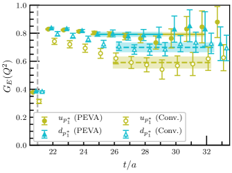
Figure 1: Quark-flavour contributions to the electric form factor for the first negative-parity excitation of the nucleon at $m_{\pi}=$702\text{\,}\mathrm{MeV}$$ for the lowest-momentum kinematics, providing $Q^{2}=$0.1424(41)\text{\,}\mathrm{G}\mathrm{eV}^{2}$$. We plot the conventional analysis with open markers and the new PEVA technique with filled markers. Our fits to the plateaus are illustrated by shaded bands, with dashed fit lines for the conventional analysis, and solid fit lines for PEVA. The source is at time slice 16, and the current is inserted at time slice 21, as indicated by the vertical dashed line. Both PEVA fits are from time slice $25$, whereas the conventional fits both start at $26$, and have significantly lower values than the PEVA fits.

IV.1.1 Quark-flavour contributions

Beginning with the lowest-lying negative-parity excitation observed in this study, we examine how extractions of ${G_{{E}}(Q^{2})}{}$ by both the PEVA technique and the conventional analysis defined in Sec. III.2 depend on the Euclidean time of the sink. In Fig. 1, we plot the connected contributions to ${G_{{E}}(Q^{2})}{}$ from single quarks of unit charge for both quark flavours present in the nucleon interpolator. This plot is at the heaviest quark mass considered with $m_{\pi}=$702\text{\,}\mathrm{MeV}$$ and the lowest-momentum kinematics of $\bm{p}=(0,0,0)$ and $\bm{p}^{\prime}=(1,0,0)$.

We see that the conventional extraction sits well below the PEVA extraction for all time slices between the current insertion and the point at which the signal is lost to noise. The conventional extraction also has a more significant time dependence than the PEVA extraction, forcing the conventional fit one time slice later. Both of these effects indicate that the conventional analysis is affected by opposite-parity contaminations, which are having a significant effect on the extracted form factor, introducing a systematic error of $12(4)\text{\,}\mathrm{\char 37\relax}$ for the singly represented quark flavour and $25(5)\text{\,}\mathrm{\char 37\relax}$ for the doubly represented flavour.

The lighter pion masses show a similar behaviour. The conventional analysis consistently has a plateau which starts later than the PEVA approach and sits significantly lower. For example, at $m_{\pi}=$411\text{\,}\mathrm{MeV}$$, the magnitudes of the conventional plateaus with these low-momentum kinematics are systematically underestimated by $19(6)\text{\,}\mathrm{\char 37\relax}$ and $26(6)\text{\,}\mathrm{\char 37\relax}$ for the singly and doubly represented quark flavours respectively.

We can also consider changing the momenta to access different kinematics. By boosting the initial and final states while keeping the momentum transfer constant, we can access smaller values of $Q^{2}$. We can also increase the three-momentum of the current insertion, giving access to larger values of $Q^{2}$. For such kinematics at all masses we find that in general, the conventional plateaus are later in time and take smaller values than the PEVA plateaus.

These results indicate that the PEVA technique is critical to the correct extraction of the electric form factors of this nucleon excitation. The conventional analysis is contaminated by opposite-parity states, and when these states are removed by the PEVA technique it has a significant effect on the extracted form factor values. Hence, we now focus our attention only on the PEVA results for the remainder of this subsection.

Table 3: Different kinematics used in our analysis to access a range of $Q^{2}$ values. The $Q^{2}$ value listed is for the first negative-parity nucleon excitation at the middle pion mass of $m_{\pi}=$411\text{\,}\mathrm{MeV}$$. The statistical error listed for $Q^{2}$ comes from both the determination of the mass of the state and the conversion to physical units. In the so-called Breit frame kinematics, where the incoming and outgoing energies are equal, the correlated statistical errors from the mass cancel exactly, and as such the only source of errors is uncertainty in the lattice spacing used in converting to physical units.

Source momentum $\bm{p}$	Sink momentum $\bm{p}^{\prime}$	Momentum transfer $\bm{q}$	$Q^{2}\,/\,$\mathrm{G}\mathrm{eV}^{2}$$
$(2,0,0)$	$(3,0,0)$	$(1,0,0)$	$0.1224$ p m 0.0035
$(2,0,1)$	$(3,0,1)$	$(1,0,0)$	$0.1239$ p m 0.0035
$(1,0,0)$	$(2,0,0)$	$(1,0,0)$	$0.1454$ p m 0.0040
$(1,0,1)$	$(2,0,1)$	$(1,0,0)$	$0.1462$ p m 0.0040
$(0,0,0)$	$(1,0,0)$	$(1,0,0)$	$0.1604$ p m 0.0044
$(0,0,1)$	$(1,0,1)$	$(1,0,0)$	$0.1606$ p m 0.0044
$(2,0,0)$	$(3,1,0)$	$(1,1,0)$	$0.2683$ p m 0.0074
$(1,0,0)$	$(2,1,0)$	$(1,1,0)$	$0.2953$ p m 0.0081
$(0,0,0)$	$(1,1,0)$	$(1,1,0)$	$0.3169$ p m 0.0086
$(0,-1,0)$	$(1,0,0)$	$(1,1,0)$	$0.3251$ p m 0.0089
$(1,0,0)$	$(3,0,0)$	$(2,0,0)$	$0.5404$ p m 0.0150
$(0,0,0)$	$(2,0,0)$	$(2,0,0)$	$0.6190$ p m 0.0169
$(-1,0,0)$	$(1,0,0)$	$(2,0,0)$	$0.6502$ p m 0.0177

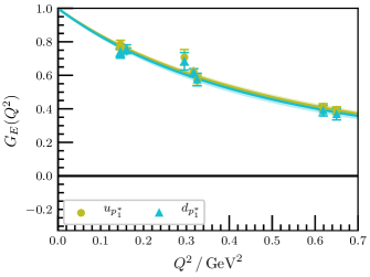
Figure 2: Quark-flavour contributions to the electric form factor for the first negative-parity excitation at $m_{\pi}=$411\text{\,}\mathrm{MeV}$$. The curves are dipole fits to the form factors, with the $y$-intercept fixed to unity. They correspond to RMS charge radii of $0.654(20)\text{\,}\mathrm{fm}$ for the doubly represented quark flavour (${u_{{p^{*}_{1}}}}$) and $0.670(26)\text{\,}\mathrm{fm}$ for the singly represented quark flavour (${d_{{p^{*}_{1}}}}$).

In Fig. 2, we plot the $Q^{2}$ dependence of the electric form factor at $m_{\pi}=$411\text{\,}\mathrm{MeV}$$. The set of kinematics used to access the various $Q^{2}$ values is listed in Table 3, and we exclude any fits for which there is no acceptable plateau, or the variational analysis fails. We see that the two quark flavours have very similar contributions to the electric form factor. They both agree well with a dipole ansatz

$${G_{{D}}(Q^{2})}{}=\frac{G_{0}{}}{{\left(1+Q^{2}/\Lambda{}^{2}\right)}^{2}}\,,$$ (13)

with $G_{0}{}$ fixed to one, as we are working with single quarks of unit charge. These fits correspond to a RMS charge radius of $0.654(20)\text{\,}\mathrm{fm}$ for the doubly represented quark flavour and $0.670(26)\text{\,}\mathrm{fm}$ for the singly represented quark flavour. These charge radii are similar to the charge radii of the individual quark sectors in the ground state examined in Ref. Stokes et al. (2019), ($0.662(12)\text{\,}\mathrm{fm}$ for the doubly represented quark flavour and $0.633(12)\text{\,}\mathrm{fm}$ for the singly represented quark flavour). The doubly represented quark sector agrees to within one standard deviation. However, the singly represented quark sector in the excitation has a charge radius approximately $1.5$ standard deviations larger than the ground state.

We see similar behaviour for the other four masses. In all cases, the quark distributions are much smaller than the lattice length $L\sim$3\text{\,}\mathrm{fm}$$. The plots for these masses are omitted from this paper for the sake of brevity.

IV.1.2 Constituent quark model expectations

Within the context of a simple constituent quark model, the near equivalence of the electric charge radii of quark sectors within the ground state nucleon and the first negative parity excitation seems truly remarkable. Considering the effective potential of the radial Schrödinger equation, one expects the repulsive centripetal term proportional to $\ell\,(\ell+1)$ to force the quarks to larger radii for odd-parity $\ell=1$ states.

However, one needs to recall that these radii are from quantum field theory where dynamical quark-antiquark pairs enable the creation of meson-nucleon components in the $N^{*}$ states. The meson provides the negative parity such that all quarks can reside in relative $s$-waves within the hadrons, forming an $S$-wave meson-baryon molecule. In this way the centripetal barrier is avoided and the negative-parity states can have a size similar to the ground state nucleon. Relevant meson-baryon channels for the odd-parity states include $K\Sigma$ and $K\Lambda$ in addition to the standard $\eta N$ and $\pi N$ meson-baryon channels.

IV.1.3 Baryon electric form factors

In order to compute the form factors of the first negative-parity excitation of the proton, ${G^{{p^{*}_{1}}}_{{E}}(Q^{2})}$, and neutron, ${G^{{n^{*}_{1}}}_{{E}}(Q^{2})}$, we need to take the correct linear combinations of the contributions from the doubly represented quark flavour and the singly represented quark flavour to reintroduce the multiplicity of the doubly represented quark and the physical charges of the up and down quarks. To this end we define

$${G^{{p^{*}_{1}}}_{{E}}(Q^{2})}{} \equiv+\frac{4}{3}{G^{{u_{{p^{*}_{1}}}}}_{{E}}(Q^{2})}{}-\frac{1}{3}{G^{{d_{{p^{*}_{1}}}}}_{{E}}(Q^{2})}{}\,,$$ (14a)

$${G^{{n^{*}_{1}}}_{{E}}(Q^{2})}{} \equiv-\frac{2}{3}{G^{{u_{{p^{*}_{1}}}}}_{{E}}(Q^{2})}{}+\frac{2}{3}{G^{{d_{{p^{*}_{1}}}}}_{{E}}(Q^{2})}{}\,.$$ (14b)

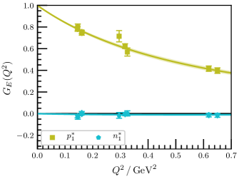
Figure 3: ${G_{{E}}(Q^{2})}$ for the first negative-parity excitations of the proton and neutron at $m_{\pi}=$411\text{\,}\mathrm{MeV}$$. The curves correspond to linear combinations of the dipole fits to the individual quark sectors from Fig. 2. These combinations provide a squared charge radius of $0.421(29)\text{\,}{\mathrm{fm}}^{2}$ for the proton and $0.014(18)\text{\,}{\mathrm{fm}}^{2}$ for the neutron.

In Fig. 3, we plot the nucleon electric form factors obtained by taking these combinations of the form factors at $m_{\pi}=$411\text{\,}\mathrm{MeV}$$. The form factor for the neutron excitation is close to zero, reflecting the similar charge radii of the individual quark flavours. By combining the dipole fits to the individual quark sectors in the same way as the data points one obtains a model for the $Q^{2}$ dependence of the electric form factors of the excited proton and neutron that includes full information from both quark sectors. If we do this for all five pion masses, we extract squared charge radii for the proton excitation ranging from $0.340(29)\text{\,}{\mathrm{fm}}^{2}$ to $0.470(54)\text{\,}{\mathrm{fm}}^{2}$, increasing with decreasing pion mass. For the neutron excitation, the squared charge radii are close to or slightly below zero, for example $-0.033(24)\text{\,}{\mathrm{fm}}^{2}$ at $m_{\pi}=$296\text{\,}\mathrm{MeV}$$.

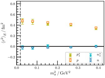
Figure 4: Quark-mass dependence of squared charge radii for the first negative-parity excitation of the proton and neutron. Results are obtained from dipole fits to the electric form factors of the individual quark sectors. For comparison, the radii for the ground states are plotted with open points. We see a clear trend to larger charge radii as the pion mass approaches the physical pion, represented by the dashed vertical line.

As illustrated in Fig. 4, the pion-mass dependence is fairly smooth, and has a clear trend to larger radii at lower pion masses. There is no hint of significant non-analytic behaviour in the quark-mass dependence, due to finite-volume suppression Hall et al. (2013b, c).

For each pion mass considered, the extracted squared charge radii for this first negative-parity excitation are consistent with the radii of the ground-state proton and neutron at the same mass, as obtained in Ref. Stokes et al. (2019).

As discussed in the context of the quark sector contributions, meson-nucleon components in the wave function enable all quarks to reside in relative $s$-waves within the hadrons, forming an $S$-wave meson-nucleon molecule. In this way, the negative-parity states can have a size similar to the ground state nucleon.

IV.2 $G_{M}$ for first negative-parity excitation

IV.2.1 Quark-flavour contributions

We now proceed to the magnetic form factor. In Fig. 5, we plot the plateaus at $m_{\pi}=$411\text{\,}\mathrm{MeV}$$ with the lowest-momentum kinematics. Here we present results in terms of nuclear magnetons, $\mu_{N}\equiv\frac{e\hbar}{2{m^{{\mathrm{{phys}}}\,{p}}}{}}$, defined in terms of the physical proton mass, ${m^{{\mathrm{{phys}}}\,{p}}}{}$. While the conventional and PEVA plateaus for the doubly represented quark flavour are consistent, both in fit region and value, the conventional plateau for the singly represented quark flavour starts later and has a significantly more negative value than the PEVA plateau. We see a similar effect at all five pion masses and a variety of kinematics.

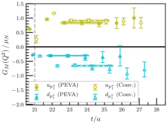
Figure 5: Quark-flavour contributions to ${G_{{M}}(Q^{2})}$ for the first negative-parity excitation at $m_{\pi}=$411\text{\,}\mathrm{MeV}$$ for the lowest-momentum kinematics, providing $Q^{2}=$0.1604(44)\text{\,}\mathrm{G}\mathrm{eV}^{2}$$. As in Fig. 1, we plot the conventional analysis with open markers and dashed fit lines and the new PEVA approach with filled markers and solid fit lines. For the doubly represented quark flavour, the plateaus for both analyses are from $23$–$25$ and take consistent values. For the singly represented quark flavour, the PEVA fit is from $22$–$24$, while the conventional fit is from $23$–$25$, and has a significantly more negative value.

Having fit the form factor plateaus, we can investigate the $Q^{2}$ dependence of ${G_{{M}}(Q^{2})}$. In Fig. 6, we plot the contributions to ${G_{{M}}(Q^{2})}$ from both the singly represented quark flavour and the doubly represented quark flavour at $m_{\pi}=$411\text{\,}\mathrm{MeV}$$. Both quark flavours are consistent with a dipole fit. The $Q^{2}$ dependence is similar to that for ${G_{{E}}(Q^{2})}$, and the same is true for the other pion masses considered.

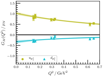
Figure 6: Quark-flavour contributions to ${G_{{M}}(Q^{2})}$ for the first negative-parity excitation at $m_{\pi}=$411\text{\,}\mathrm{MeV}$$. The curves are dipole fits to the individual quark sectors.

IV.2.2 Baryon magnetic form factors

As described in Section IV.1, we can take linear combinations of the individual quark flavour contributions to compute the magnetic form factors of the excited proton and neutron. We plot these combinations for $m_{\pi}=$411\text{\,}\mathrm{MeV}$$ in Fig. 7. The squared magnetic radii given by

$$\frac{{\braket{r^{2}}_{{M}}}{}}{{\mu}{}}=\frac{-6}{{G_{{M}}(0)}{}}\,{\left.\frac{d{G_{{M}}(Q^{2})}{}}{dQ^{2}}\right|}_{Q^{2}=0}\,,$$ (15)

are obtained via dipole fits to the quark sector contributions, which allow the value and slope of ${G_{{M}}(Q^{2})}{}$ to be extrapolated to $Q^{2}=0$. In obtaining hadronic magnetic radii, the quark sectors combine with additional weightings given by ${G_{{M}}(0)}{}$, that is

$$\frac{{\braket{r^{2}}^{{p^{*}_{1}}}_{{M}}}{}}{{\mu^{{p^{*}_{1}}}}{}} \equiv\frac{1}{+\frac{4}{3}{G^{{u_{{p^{*}_{1}}}}}_{{M}}(0)}{}-\frac{1}{3}{G^{{d_{{p^{*}_{1}}}}}_{{M}}(0)}{}}$$

$$\!\!\!\!\!\!\!\!\!\!\!\times\!\left(+\frac{4}{3}{G^{{u_{{p^{*}_{1}}}}}_{{M}}(0)}{}\frac{{\braket{r^{2}}^{{u_{{p^{*}_{1}}}}}_{{M}}}{}}{{\mu^{{u_{{p^{*}_{1}}}}}}{}}-\frac{1}{3}{G^{{d_{{p^{*}_{1}}}}}_{{M}}(0)}{}\frac{{\braket{r^{2}}^{{d_{{p^{*}_{1}}}}}_{{M}}}{}}{{\mu^{{d_{{p^{*}_{1}}}}}}{}}\right),$$ (16a)

$$\frac{{\braket{r^{2}}^{{n^{*}_{1}}}_{{M}}}{}}{{\mu^{{n^{*}_{1}}}}{}} \equiv\frac{1}{-\frac{2}{3}{G^{{u_{{p^{*}_{1}}}}}_{{M}}(0)}{}+\frac{2}{3}{G^{{d_{{p^{*}_{1}}}}}_{{M}}(0)}{}}$$

$$\!\!\!\!\!\!\!\!\!\!\!\times\!\left(-\frac{2}{3}{G^{{u_{{p^{*}_{1}}}}}_{{M}}(0)}{}\frac{{\braket{r^{2}}^{{u_{{p^{*}_{1}}}}}_{{M}}}{}}{{\mu^{{u_{{p^{*}_{1}}}}}}{}}+\frac{2}{3}{G^{{d_{{p^{*}_{1}}}}}_{{M}}(0)}{}\frac{{\braket{r^{2}}^{{d_{{p^{*}_{1}}}}}_{{M}}}{}}{{\mu^{{d_{{p^{*}_{1}}}}}}{}}\right).$$ (16b)

For all five masses, we find that these squared magnetic radii mostly agree with the charge radii from ${G_{{E}}(Q^{2})}$.

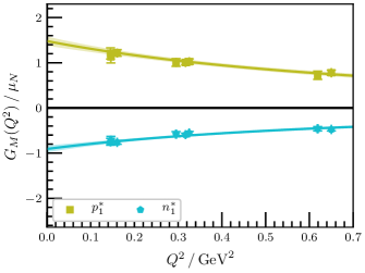
Figure 7: ${G_{{M}}(Q^{2})}$ for the first negative-parity excitations of the proton and neutron at $m_{\pi}=$411\text{\,}\mathrm{MeV}$$. The curves correspond to linear combinations of the quark-sector dipole fits from Fig. 6.

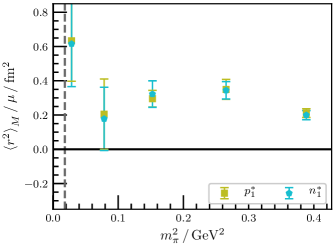
Figure 8: Quark-mass dependence of squared magnetic radii for the first negative-parity excitation of the proton.

In Fig. 8, we plot the pion-mass dependence of the squared magnetic radius obtained from quark-sector dipole fits to ${G_{{M}}(Q^{2})}$ for the excited proton and neutron.

IV.2.3 Baryon magnetic moments

Returning to the individual quark sector results, we note that ${G_{{M}}(Q^{2})}$ and ${G_{{E}}(Q^{2})}$ have a similar $Q^{2}$ dependence over the range considered. In light of this, we hypothesise that ${G_{{M}}(Q^{2})}{}$ and ${G_{{E}}(Q^{2})}{}$ have the same $Q^{2}$ scaling in this region. If this hypothesis is valid, then the ratio of ${G_{{M}}(Q^{2})}{}$ to ${G_{{E}}(Q^{2})}{}$ should be independent of $Q^{2}$. Since we are working with an improved conserved vector current, and single quarks of unit charge, ${G_{{E}}(0)}{}=1$ exactly, and ${G_{{M}}(0)}{}$ is the contribution of the quark flavour to the magnetic moment (up to scaling by the physical charge). Hence, the ratio

$${\mu_{{\mathrm{{eff}}}}}{}(Q^{2})\equiv\frac{{G_{{M}}(Q^{2})}{}}{{G_{{E}}(Q^{2})}{}}\,,$$ (17)

is expected to provide a measure of the contribution to the magnetic moment from the given quark flavour.

In Fig. 9, we plot this ratio at $m_{\pi}=$411\text{\,}\mathrm{MeV}$$ as a function of $Q^{2}$. We see that as expected, the ratio is approximately constant across the $Q^{2}$ range accessible by our kinematics. This holds true for all five pion masses considered in this work. This supports the underlying hypothesis that the $Q^{2}$ scaling of the contributions to ${G_{{E}}(Q^{2})}$ and ${G_{{M}}(Q^{2})}$ from each quark sector is the same, and hence suggests that ${\mu_{{\mathrm{{eff}}}}}{}$ is a good estimate for the magnetic moment of this state.

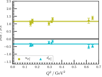
Figure 9: ${\mu_{{\mathrm{{eff}}}}}{}$ for individual quarks of unit charge in the first negative-parity nucleon excitation at $m_{\pi}=$411\text{\,}\mathrm{MeV}$$. The shaded bands are constant fits to the effective magnetic moment, corresponding to magnetic moment contributions of $1.163(60)$ $\mu_{N}$ for the doubly represented quark and $-0.333(43)$ $\mu_{N}$ for the singly represented quark.

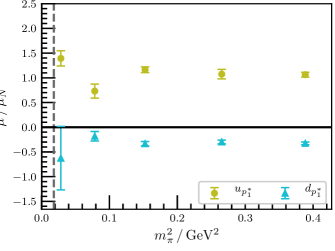
Figure 10: Quark-mass dependence of contributions from individual unit-charge quarks to the magnetic moment of the first negative-parity nucleon excitation. The vertical dashed line corresponds to the physical pion mass.

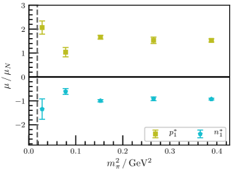
Figure 11: Quark-mass dependence of the magnetic moment of the first negative-parity excitations of the proton and neutron.

We take constant fits to ${\mu_{{\mathrm{{eff}}}}}$ at each quark mass, and plot their pion-mass dependence in Fig. 10. By taking linear combinations of these fits as described for ${G_{{E}}(Q^{2})}$ and ${G_{{M}}(Q^{2})}$ above, we obtain magnetic moment estimates for the excited proton and neutron, as plotted in Fig. 11. For the heaviest three pion masses, the effective magnetic moments show little pion mass dependence and have tight error bars. The lightest two pion masses have much larger errors, and we observe a discontinuity in ${G_{{M}}(Q^{2})}$ at the the second lightest mass, appearing as a significantly smaller magnetic moment for both states. This suggests that there could be a change in the structure of this state at that mass. However, there is no corresponding change in ${G_{{E}}(Q^{2})}{}$. At the lightest mass, the magnetic moments appear to return to consistency with the values from the heavier masses. Hence, it is unclear whether the behaviour at the second lightest mass indicates a change in the nature of the state, the presence of significant scattering-state contamination, or is a result of increasing gauge noise at lighter pion masses. Further research will be required to determine which of these possibilities is realised.

In this section focusing on the first negative-parity excitation of the nucleon, we have demonstrated the importance of the PEVA technique in correctly extracting both the electric and magnetic form factors. From these, we derived charge radii, magnetic moments and magnetic radii.

While we regard the results for the three heaviest quark masses to be robust, we take some caution with the lightest quark mass results as they may be influenced by important unaccounted scattering-state contributions.

Table 4: Radii and magnetic moments of the ground state proton and neutron. Radii are obtained from from combinations of quark-sector dipole fits and magnetic moments are obtained from quark-sector ratios of ${G_{{M}}(Q^{2})}$ to ${G_{{E}}(Q^{2})}{}$.

$m_{\pi}^{2}\,/\,$\mathrm{G}\mathrm{eV}^{2}$$	${\braket{r^{2}}^{{p}}_{{E}}}{}\,/\,${\mathrm{fm}}^{2}$$	${\braket{r^{2}}^{{p}}_{{M}}}{}\,/\,{\mu^{{p}}}{}\!\,/\,${\mathrm{fm}}^{2}$$	${\mu^{{p}}}{}\!\,/\,\mu_{N}$
$0.3884$ p m 0.0113	$0.351$ p m 0.013	$0.301$ p m 0.013	$1.89$ p m 0.03
$0.2654$ p m 0.0081	$0.417$ p m 0.017	$0.341$ p m 0.015	$2.10$ p m 0.04
$0.1525$ p m 0.0043	$0.451$ p m 0.018	$0.340$ p m 0.013	$2.24$ p m 0.04
$0.0784$ p m 0.0025	$0.472$ p m 0.017	$0.360$ p m 0.016	$2.30$ p m 0.04
$0.0285$ p m 0.0012	$0.479$ p m 0.027	$0.324$ p m 0.036	$2.52$ p m 0.08

$m_{\pi}^{2}\,/\,$\mathrm{G}\mathrm{eV}^{2}$$	${\braket{r^{2}}^{{n}}_{{E}}}{}\,/\,${\mathrm{fm}}^{2}$$	${\braket{r^{2}}^{{n}}_{{M}}}{}\,/\,{\mu^{{n}}}{}\!\,/\,${\mathrm{fm}}^{2}$$	${\mu^{{n}}}{}\!\,/\,\mu_{N}$
$0.3884$ p m 0.0113	$-0.009$ p m 0.003	$0.303$ p m 0.013	$-1.20$ p m 0.02
$0.2654$ p m 0.0081	$-0.019$ p m 0.005	$0.337$ p m 0.015	$-1.33$ p m 0.03
$0.1525$ p m 0.0043	$-0.025$ p m 0.006	$0.350$ p m 0.014	$-1.38$ p m 0.03
$0.0784$ p m 0.0025	$-0.023$ p m 0.005	$0.376$ p m 0.020	$-1.40$ p m 0.03
$0.0285$ p m 0.0012	$-0.022$ p m 0.009	$0.437$ p m 0.084	$-1.57$ p m 0.05

Table 5: Radii and magnetic moments of the first negative parity excitation of the proton and neutron. Radii are obtained from from combinations of quark-sector dipole fits and magnetic moments are obtained from quark-sector ratios of ${G_{{M}}(Q^{2})}$ to ${G_{{E}}(Q^{2})}{}$.

$m_{\pi}^{2}\,/\,$\mathrm{G}\mathrm{eV}^{2}$$	${\braket{r^{2}}^{{p^{*}_{1}}}_{{E}}}{}\,/\,${\mathrm{fm}}^{2}$$	${\braket{r^{2}}^{{p^{*}_{1}}}_{{M}}}{}\,/\,{\mu^{{p^{*}_{1}}}}{}\!\,/\,${\mathrm{fm}}^{2}$$	${\mu^{{p^{*}_{1}}}}{}\!\,/\,\mu_{N}$
$0.3884$ p m 0.0113	$0.340$ p m 0.029	$0.21$ p m 0.03	$1.53$ p m 0.07
$0.2654$ p m 0.0081	$0.403$ p m 0.024	$0.35$ p m 0.06	$1.53$ p m 0.14
$0.1525$ p m 0.0043	$0.421$ p m 0.029	$0.30$ p m 0.05	$1.66$ p m 0.08
$0.0784$ p m 0.0025	$0.462$ p m 0.050	$0.21$ p m 0.21	$1.04$ p m 0.20
$0.0285$ p m 0.0012	$0.470$ p m 0.054	$0.63$ p m 0.24	$2.07$ p m 0.28

$m_{\pi}^{2}\,/\,$\mathrm{G}\mathrm{eV}^{2}$$	${\braket{r^{2}}^{{n^{*}_{1}}}_{{E}}}{}\,/\,${\mathrm{fm}}^{2}$$	${\braket{r^{2}}^{{n^{*}_{1}}}_{{M}}}{}\,/\,{\mu^{{n^{*}_{1}}}}{}\!\,/\,${\mathrm{fm}}^{2}$$	${\mu^{{n^{*}_{1}}}}{}\!\,/\,\mu_{N}$
$0.3884$ p m 0.0113	$0.007$ p m 0.015	$0.20$ p m 0.03	$-0.93$ p m 0.04
$0.2654$ p m 0.0081	$-0.016$ p m 0.012	$0.34$ p m 0.05	$-0.92$ p m 0.08
$0.1525$ p m 0.0043	$0.014$ p m 0.018	$0.32$ p m 0.08	$-1.00$ p m 0.05
$0.0784$ p m 0.0025	$-0.033$ p m 0.024	$0.18$ p m 0.18	$-0.61$ p m 0.12
$0.0285$ p m 0.0012	$-0.021$ p m 0.036	$0.62$ p m 0.25	$-1.35$ p m 0.43

In Table 4, we present the charge radii, magnetic radii, and magnetic moments of the ground state proton and neutron. These measurements are obtained from the electric and magnetic form factors as described above. We provide these results here for easy comparison with the excited state results presented in this paper.

In Table 5, we present the same results for the first negative-parity excitation. We see that this state has radii similar to the ground state, but notably different magnetic moments. We find that at the heavier quark masses, these magnetic moments agree well with constituent quark model predictions, as discussed below in Section IV.5.

IV.3 $G_{E}$ for the second negative-parity excitation

IV.3.1 Quark-flavour contributions

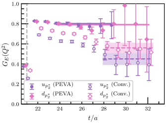
Figure 12: Quark-flavour contributions to the electric form factor for the second negative-parity nucleon excitation at $m_{\pi}=$702\text{\,}\mathrm{MeV}$$ for the lowest-momentum kinematics, providing $Q^{2}=$0.1425(41)\text{\,}\mathrm{G}\mathrm{eV}^{2}$$. We plot the conventional analysis with open markers and dashed fit lines and the new PEVA approach with filled markers and solid fit lines. Results for both the singly represented quark flavour (${d_{{p^{*}_{2}}}}$) and the doubly represented quark flavour (${u_{{p^{*}_{2}}}}$) are shown for single quarks of unit charge. Both PEVA fits are from time slice $24$, whereas the conventional fits both start at time slice $28$. The values for both conventional fits are significantly lower than the corresponding PEVA fits.

We now proceed to examine the next negative-parity excitation observed in this study, ${N^{*}_{2}\!}$. In Fig. 12, we plot ${G_{{E}}(Q^{2})}{}$ as a function of sink time for both quark flavours at $m_{\pi}=$702\text{\,}\mathrm{MeV}$$ with the lowest-momentum kinematics. We see that the conventional extraction sits even further below the PEVA extraction than the first negative-parity excitation. While the PEVA fits start at time slice $24$, the conventional fits are forced all the way out to time slice $28$ and sit at only just above half of the values of the PEVA fits.

Moving on to the lighter pion masses, the discrepancy between the extracted form factors continues at $m_{\pi}=$570\text{\,}\mathrm{MeV}$$ and $411\text{\,}\mathrm{MeV}$, with the conventional analysis giving consistently lower values than PEVA. For example, Fig. 13 shows the plateaus at $m_{\pi}=$570\text{\,}\mathrm{MeV}$$.

At the lightest two pion masses, the signal gets significantly noisier, and the difference between the two techniques gets harder to distinguish. Increased statistics are required in order to clearly identify the effects of opposite-parity contaminations of this state at these masses. However, in principle, the enhancement of relativistic components of the baryon spinors at light quark masses is expected to increase parity mixing in the conventional analysis.

In addition, in the tail of the two point correlation function at the lightest mass, contributions from low-lying states are evident from a $\chi^{2}$ analysis of a single state ansatz. This effect was also seen in Ref. Mahbub et al. (2014), where it was found that so long as a single-state ansatz is satisfied in the fit region, this contamination does not have a significant effect on the extracted mass. However, as shown in Ref. Stokes et al. (2019), contaminants that do not significantly perturb the extracted mass can still have a significant effect on the extracted form factors. As such, we must be cautious when interpreting results from this state at this mass. To gain a deeper insight into this state at this mass, multi-particle scattering operators will be necessary to properly isolate the low-lying scattering state.

Returning to the other ensembles, we find that the trends from the lowest-momentum kinematics continue for all other kinematics: for all masses for which the noise is sufficiently low, the conventional fits sit significantly lower than the PEVA fits.

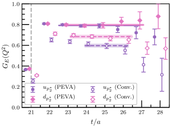
Figure 13: Quark-flavour contributions to ${G_{{E}}(Q^{2})}$ for the second negative-parity excitation at $m_{\pi}=$570\text{\,}\mathrm{MeV}$$ for the lowest-momentum kinematics, providing $Q^{2}=$0.1458(44)\text{\,}\mathrm{G}\mathrm{eV}^{2}$$. The conventions used in this plot are the same as in Fig. 12. The conventional fits have significantly lower values than the PEVA fits, and the plateau for the doubly represented quark flavour starts one time slice later than the corresponding PEVA plateau.

Once again, these results clearly indicate that PEVA is critical to the correct extraction of the electric form factors of this nucleon excitation. The opposite-parity contaminations admitted by the conventional analysis lead to significant underestimation of the value of the electric form factor. Hence, we now focus our attention only on the PEVA results.

Plotting the acceptable plateaus as a function of $Q^{2}$ reveals that the contributions from the two quark flavours are once again very similar, and agree well with a dipole ansatz. For example, Fig. 14 shows dipole fits to the two quark flavours at $m_{\pi}=$411\text{\,}\mathrm{MeV}$$, with a RMS charge radius of $0.679(38)\text{\,}\mathrm{fm}$ for the doubly represented quark flavour and $0.715(31)\text{\,}\mathrm{fm}$ for the singly represented quark flavour.

The charge radius of the doubly represented quark flavour of $0.679(38)\text{\,}\mathrm{fm}$ is similar to that seen in the ground state, $0.662(12)\text{\,}\mathrm{fm}$ Stokes et al. (2019) again suggesting a role for meson-baryon contributions escaping the centripetal barrier encountered in a three-quark composition. This time the RMS charge radius of the singly represented quark flavour of $0.715(31)\text{\,}\mathrm{fm}$ is larger that that observed in the ground state, $0.633(12)\text{\,}\mathrm{fm}$. However, it does overlap with that of the first negative parity excitation at the one-sigma level.

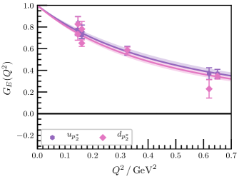
Figure 14: Quark-flavour contributions to ${G_{{E}}(Q^{2})}$ for the second negative-parity excitation at $m_{\pi}=$411\text{\,}\mathrm{MeV}$$. The curves are dipole fits to the form factor, with the $y$-intercept fixed to unity. They correspond to RMS charge radii of $0.679(38)\text{\,}\mathrm{fm}$ for the doubly represented quark (${u_{{p}}}$) and $0.715(31)\text{\,}\mathrm{fm}$ for the singly represented quark (${d_{{p}}}$).

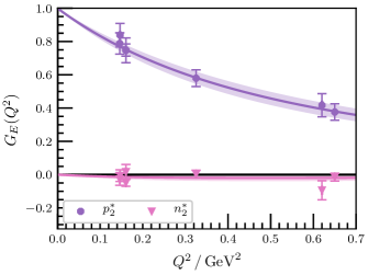
Figure 15: ${G_{{E}}(Q^{2})}$ for the second negative-parity excitation of the proton and neutron at $m_{\pi}=$411\text{\,}\mathrm{MeV}$$. The curves correspond to combinations of the quark-sector dipole fits from Fig. 14, giving squared charge radii of $0.445(62)\text{\,}{\mathrm{fm}}^{2}$ for the excited proton and $0.033(30)\text{\,}{\mathrm{fm}}^{2}$ for the excited neutron.

IV.3.2 Baryon electric form factors

We once again take the linear combinations discussed in Section IV.1 to form the excited proton and neutron. For example, in Fig. 15, we plot the electric form factors obtained from the quark-sector combinations at $m_{\pi}=$411\text{\,}\mathrm{MeV}$$. At all five masses, the electric form factor for the second negative-parity excitation of the neutron is approximately zero.

The pion-mass dependence of the charge radii is illustrated in Fig. 16. At the heaviest three pion masses, the linear combinations of the quark-sector dipole fits once again provide charge radii consistent with the ground-state nucleon at the same quark mass Stokes et al. (2019), pointing to a role for meson-baryon $S$-wave Fock-space components, escaping the centripetal barrier encountered in a three-quark composition. We see that the pion-mass dependence of the proton radius is fairly smooth at these heaviest masses, and has a clear trend to increasing charge radius at lower pion masses.

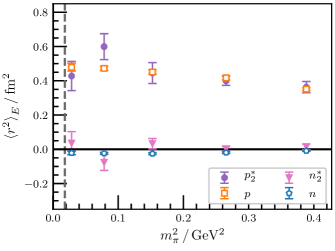
Figure 16: Quark-mass dependence of charge radii from combinations of quark-sector dipole fits to ${G_{{E}}(Q^{2})}$ for the second negative-parity excitation of the proton and neutron. The vertical dashed line corresponds to the physical pion mass, and the ground state is plotted with open points for comparison.

IV.4 $G_{M}$ for the second negative-parity excitation

IV.4.1 Quark-flavour contributions

We now advance to the magnetic form factor of this state. In Fig. 17, we plot the heaviest pion mass of $m_{\pi}=$702\text{\,}\mathrm{MeV}$$ and the lowest-momentum kinematics. While the plateau time-regions for the PEVA and conventional analysis are consistent, the values of those plateaus are very different, and in fact change ordering between the two extractions. We see a similar effect at $m_{\pi}=$296\text{\,}\mathrm{MeV}$$, $411\text{\,}\mathrm{MeV}$, and $570\text{\,}\mathrm{MeV}$, with similar inversions of the magnetic form factors between the two analyses. We see similar patterns for the other kinematics, with significantly different plateau values between the two analyses when the statistical noise is low enough to distinguish them.

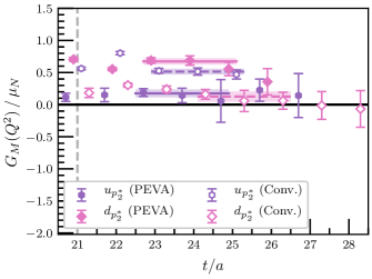
Figure 17: Quark-flavour contributions to ${G_{{M}}(Q^{2})}$ for the second negative-parity excitation of the nucleon at $m_{\pi}=$702\text{\,}\mathrm{MeV}$$ for the lowest-momentum kinematics, providing $Q^{2}=$0.1425(41)\text{\,}\mathrm{G}\mathrm{eV}^{2}$$. The conventions used in this plot are the same as in Fig. 12. The plateaus for the PEVA technique both start at time slice $23$. The plateaus for the conventional analysis start at time slice $23$ for ${u_{{p^{*}_{2}}}}$ and time slice $24$ for ${d_{{p^{*}_{2}}}}$. The difference in the plateau values between the two analyses is enough to change the ordering of the two quark flavours.

Once again the PEVA technique is crucial to extracting the correct form factors. Hence, we focus only on the PEVA results. Inspecting the $Q^{2}$ dependence of these form factors, we find that the contributions from both quark flavours agree well with a dipole ansatz. For example, Fig. 18 shows the form factors at $m_{\pi}=$411\text{\,}\mathrm{MeV}$$. Here we have held the $y$-scale fixed to match previous plots, for ease of comparison. The most notable feature of these results is their small magnitude compared to the both the ground state and the excitation considered in Section IV.2.

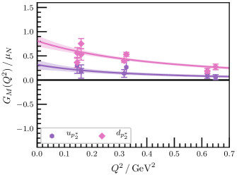
Figure 18: Quark-flavour contributions to ${G_{{M}}(Q^{2})}$ for the second negative-parity excitation at $m_{\pi}=$411\text{\,}\mathrm{MeV}$$. The curves are dipole fits to the individual quark sectors.

IV.4.2 Baryon magnetic form factors

By taking linear combinations based on the multiplicity and charge of each quark flavour, as described in Section IV.1, we can obtain the magnetic form factors for the excited proton and neutron. Fig. 19 shows these combinations for $m_{\pi}=$411\text{\,}\mathrm{MeV}$$. The magnetic charge radii obtained by combining the quark-sector dipoles are consistent with the proton charge radii from ${G_{{E}}(Q^{2})}$, although they often have very large errors due to the very small values of the magnetic form factors amplifying the effects of statistical fluctuations.

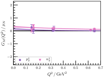
Figure 19: ${G_{{M}}(Q^{2})}$ for the excited proton and neutron at $m_{\pi}=$411\text{\,}\mathrm{MeV}$$. The curves correspond to combinations of the quark-sector dipole fits from Fig. 18.

IV.4.3 Baryon magnetic moments

Returning to the individual quark sector results with unit charge, and noting that the $Q^{2}$ dependence for ${G_{{E}}(Q^{2})}{}$ and ${G_{{M}}(Q^{2})}{}$ is similar, we once again take the ratio ${\mu_{{\mathrm{{eff}}}}}{}(Q^{2})\equiv{G_{{M}}(Q^{2})}{}/{G_{{E}}(Q^{2})}{}$. We find that this ratio is approximately flat for all five pion masses. For example, Fig. 20 shows the $Q^{2}$ dependence of the ratio at $m_{\pi}=$411\text{\,}\mathrm{MeV}$$. We can extract the contributions to the magnetic moment from both quark flavours from constant fits to this ratio.

Fig. 21 shows the pion-mass dependence of these extracted magnetic moment contributions. It is remarkable that both quark flavours contribute with the same sign.

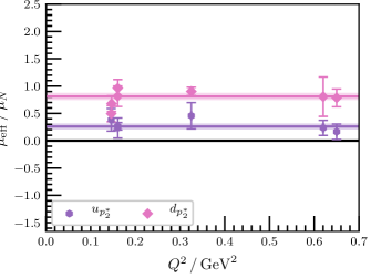
Figure 20: ${\mu_{{\mathrm{{eff}}}}}{}$ for individual quarks of unit charge in the second negative-parity excitation at $m_{\pi}=$411\text{\,}\mathrm{MeV}$$. The shaded bands are constant fits to the effective magnetic moment, corresponding to magnetic moment contributions of $0.260(55)$ $\mu_{N}$ for the doubly represented quark and $0.810(67)$ $\mu_{N}$ for the singly represented quark.

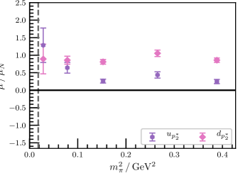
Figure 21: Quark-mass dependence of contributions from individual unit-charge quarks to the magnetic moment of the second negative-parity excitation of the nucleon. The vertical dashed line corresponds to the physical pion mass.

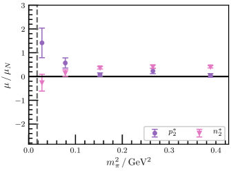
Figure 22: Quark-mass dependence of the magnetic moment of the second negative-parity excitations of the proton and neutron. The dashed line corresponds to the physical pion mass. There is a clear change at the lightest two pion masses, which signals a significant shift in the structure of the states.

By taking the linear combinations discussed above, we can combine these individual quark flavour results to get the predicted magnetic moments for the second negative-parity excitations of the proton and neutron. In Fig. 22 we plot the dependence of these combinations on the squared pion mass. For the heaviest three pion masses, the effective magnetic moments show little pion mass dependence and have tight error bars. The magnetic moment of the proton excitation sits very close to zero, and the magnetic moment of the neutron excitation has a small but nonzero positive value. For the lightest two masses, the ordering of the two states flips, with the proton excitation taking on a more significant magnetic moment, and the neutron excitation dropping to be consistent with or below zero.

In summary, the PEVA technique is crucial for extracting both the electric and magnetic form factors of the second negative-parity excitations of the proton and neutron. In Table 6, we present the charge radii, magnetic radii, and magnetic moments of the second negative-parity excitation of the proton and neutron. We see that this state has similar radii to the ground state, but notably different magnetic moments. We find that at the heavier quark masses, these magnetic moments agree well with constituent quark model predictions, as discussed below.

Table 6: Radii and magnetic moments of the second negative-parity excitation of the proton and neutron. Radii are obtained from from combinations of quark-sector dipole fits and magnetic moments are obtained from quark-sector ratios of ${G_{{M}}(Q^{2})}$ to ${G_{{E}}(Q^{2})}{}$. At the lightest two pion masses, the form factor data was insufficient to properly constrain a dipole fit so we do not report magnetic radii at these masses.

$m_{\pi}^{2}\,/\,$\mathrm{G}\mathrm{eV}^{2}$$	${\braket{r^{2}}^{{p^{*}_{2}}}_{{E}}}{}\,/\,${\mathrm{fm}}^{2}$$	${\braket{r^{2}}^{{p^{*}_{2}}}_{{M}}}{}\,/\,{\mu^{{p^{*}_{2}}}}{}\!\,/\,${\mathrm{fm}}^{2}$$	${\mu^{{p^{*}_{2}}}}{}\!\,/\,\mu_{N}$
$0.3884$ p m 0.0113	$0.363$ p m 0.035	$0.56$ p m 2.13	$0.05$ p m 0.08
$0.2654$ p m 0.0081	$0.399$ p m 0.029	$0.55$ p m 0.70	$0.23$ p m 0.11
$0.1525$ p m 0.0043	$0.445$ p m 0.062	$1.09$ p m 0.70	$0.08$ p m 0.07
$0.0784$ p m 0.0025	$0.599$ p m 0.077	—	$0.57$ p m 0.21
$0.0285$ p m 0.0012	$0.428$ p m 0.086	—	$1.41$ p m 0.62

$m_{\pi}^{2}\,/\,$\mathrm{G}\mathrm{eV}^{2}$$	${\braket{r^{2}}^{{n^{*}_{2}}}_{{E}}}{}\,/\,${\mathrm{fm}}^{2}$$	${\braket{r^{2}}^{{n^{*}_{2}}}_{{M}}}{}\,/\,{\mu^{{n^{*}_{2}}}}{}\!\,/\,${\mathrm{fm}}^{2}$$	${\mu^{{n^{*}_{2}}}}{}\!\,/\,\mu_{N}$
$0.3884$ p m 0.0113	$0.014$ p m 0.017	$0.30$ p m 0.18	$0.41$ p m 0.05
$0.2654$ p m 0.0081	$0.003$ p m 0.014	$0.65$ p m 0.30	$0.41$ p m 0.07
$0.1525$ p m 0.0043	$0.033$ p m 0.030	$0.41$ p m 0.34	$0.37$ p m 0.05
$0.0784$ p m 0.0025	$-0.076$ p m 0.047	—	$0.14$ p m 0.14
$0.0285$ p m 0.0012	$0.036$ p m 0.068	—	$-0.26$ p m 0.35

IV.5 Model comparison

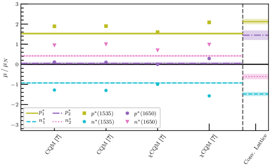
Figure 23: Comparison between lattice calculations of the magnetic moments of two negative-parity nucleon excitations at $m_{\pi}=$702\text{\,}\mathrm{MeV}$$ and quark model predictions for the $N^{*}(1535)$ and $N^{*}(1650)$ resonances . The shaded bands on the left-hand side of the plot indicate the magnetic moments calculated via the PEVA technique, and symbols denote the quark model predictions. Lattice calculations of the magnetic moments using a conventional variational analysis are plotted to the right of the vertical dashed line.

In Section I, we introduced the two low-lying negative-parity excitations of the proton and neutron observed on the lattice by the CSSM and the HSC collaborations. We wish to examine the extent to which these states, formed in relativistic quantum field theory, have properties that are captured in simple quark models. As these states have good overlap with local three-quark operators, we anticipate these states may resemble the quark-model states postulated to describe these resonances Chiang et al. (2003); Liu et al. (2005); Sharma et al. (2013).

Already we have seen some deviations from quark model expectations for electric charge radii. There, larger radii for the $N^{*}$ states were anticipated due to centripetal repulsion in the radial Schrödinger equation for three-quark states with orbital angular momentum $\ell=1$. However, similar charge radii point to five-quark meson-baryon components in the $N^{*}$ structure where the anti-quark provides negative parity and all quarks can sit in relative $s$ waves.

Here, we focus on the magnetic moments of these two negative-parity states, as calculated in sections IV.2 and IV.4. It will be interesting to learn if there is a nontrivial role for meson-baryon Fock-space components here as well.

Our focus on the three heavier quark masses considered is beneficial in comparing with quark models as it is this regime where constituent quark phenomenology is expected to be manifest Leinweber et al. (1991); Leinweber (1992).

We consider two constituent quark model (QM) predictions of the magnetic moments from Refs. Chiang et al. (2003); Liu et al. (2005), and two chiral constituent quark model ($\chi$QM) calculations which take the quark model calculations and include effects from the pion cloud Liu et al. (2005); Sharma et al. (2013), thus incorporating meson-baryon Fock-space components.

In Fig. 23, we compare our magnetic moments extracted at $m_{\pi}=$702\text{\,}\mathrm{MeV}$$ with these quark model predictions, which are calculated at the physical point. We can see that qualitatively, the results for the first negative-parity lattice excitation match up with the quark model $N^{*}(1535)$, and the second negative-parity lattice excitation with the quark model $N^{*}(1650)$. In fact, despite being at significantly different pion masses, the results are quantitatively very similar, with the lattice results sitting within the scatter of the model predictions for all states save the second negative-parity nucleon excitation, which sits slightly below all of the model predictions.

For comparison, we also plot lattice results produced using the conventional variational analysis. For these results, ${\mu_{{\mathrm{{eff}}}}}{}(Q^{2})$ varies significantly for different kinematics, so rather than taking a constant fit across kinematics, we present only the result from the lowest-momentum ($\bm{p}=(0,0,0)$, $\bm{p}^{\prime}=(1,0,0)$) kinematics, which we expect to have the smallest opposite-parity contaminations. We see that the conventional results are significantly different to the PEVA results. In particular, the conventional extraction of the second negative-parity excitation is completely different to both the PEVA result and the quark model results. This once again demonstrates how critical the PEVA technique is to obtaining correct results.

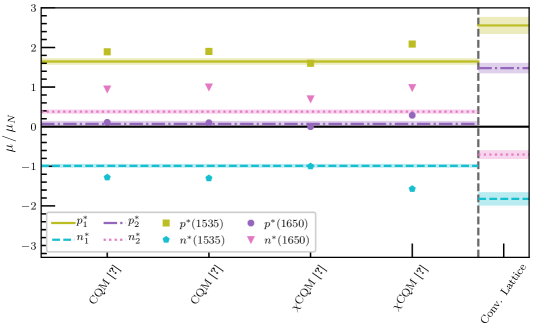
Figure 24: Comparison between magnetic moments from lattice calculations at $m_{\pi}=$411\text{\,}\mathrm{MeV}$$ and quark model predictions for the $N^{*}(1535)$ and $N^{*}(1650)$. The shaded bands indicate the PEVA calculations on the left, and the conventional analysis on the right. The markers show the quark model predictions.

This trend continues for $m_{\pi}=$570\text{\,}\mathrm{MeV}$$, and $m_{\pi}=$411\text{\,}\mathrm{MeV}$$, the latter shown in Fig. 24. Since the pion-mass dependence of the magnetic moments between these three masses is quite small, the quantitative agreement remains good.

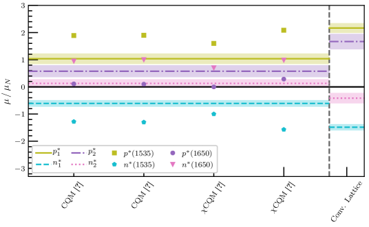
Figure 25: Comparison between magnetic moments from lattice calculations at $m_{\pi}=$296\text{\,}\mathrm{MeV}$$ and quark model predictions for the $N^{*}(1535)$ and $N^{*}(1650)$. The shaded bands indicate the PEVA calculations on the left, and the conventional analysis on the right. The markers show the quark model predictions.

For completeness, we also present a comparison for the second lightest mass. Fig. 25 shows that the lattice results depart from the model predictions at $m_{\pi}=$296\text{\,}\mathrm{MeV}$$. Again, an analysis of possible scattering-state contributions to the correlation functions is required to disentangle interesting meson-cloud effects from scattering-state contaminations as discussed in Sec. III.4. Fig. 25 also shows that there is still a significant disagreement between the conventional and PEVA results at $m_{\pi}=$296\text{\,}\mathrm{MeV}$$. It remains clear that the PEVA technique is playing an important role in addressing opposite parity contaminations.

The results presented in this section provide new insight into the structure of the negative-parity nucleon excitations observed in lattice quantum field theory. At the heavier quark masses considered, the two negative-parity excitations agree well with quark-model descriptions for the $N^{*}(1535)$ and $N^{*}(1650)$. Coupled with the charge radii from Section IV.1, which indicate the importance of meson-nucleon components in the wave function, and the observed single-particle dispersion relations seen in Ref. Stokes et al. (2015), the results indicate that these states are similar in structure to the ground state nucleon which can also be modelled as a three-quark state dressed by a meson cloud.

V Positive parity excitation

We now move to the positive parity sector, studying the first localised positive-parity excitation of the nucleon observed on the lattice. This state sits at an effective mass of approximately $2\text{\,}\mathrm{GeV}$ for all five pion masses, well above $1.43(2)\text{\,}\mathrm{GeV}$, the mass of the Roper resonance observed in nature Patrignani et al. (2016). This has long been a puzzle for the particle physics community, but recent HEFT results indicate that the Roper resonance is dynamically generated from meson-baryon scattering states Liu et al. (2017a), and hence the lattice spectrum in this energy region has poor overlap with local three-quark operators. This means that the lattice state studied here is likely associated with the $N^{*}(1710)$, $N^{*}(1880)$, and/or $N^{*}(2100)$ resonances.

V.1 Electric form factor

V.1.1 Quark-flavour contributions

We plot the dependence of ${G_{{E}}(Q^{2})}$ on the Euclidean sink time at $m_{\pi}=$702\text{\,}\mathrm{MeV}$$ in Figs. 26 and 27. The form factor values extracted from the PEVA and conventional analyses for each sink time look very similar, and this is reflected in the fits. The conventional and PEVA extractions both have clear plateaus over the same range of sink times, and these plateaus have consistent values.

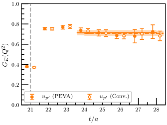
Figure 26: Contributions to ${G_{{E}}(Q^{2})}$ from the doubly represented quark flavour for the first positive-parity nucleon excitation at $m_{\pi}=$702\text{\,}\mathrm{MeV}$$ with the lowest-momentum kinematics, providing $Q^{2}=$0.1425(41)\text{\,}\mathrm{G}\mathrm{eV}^{2}$$. We plot the conventional analysis with open markers and dashed fit lines and the PEVA technique with filled markers and solid fit lines. Both fits are from time slice $24$–$28$.

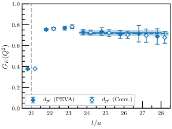
Figure 27: Contributions to ${G_{{E}}(Q^{2})}$ from the singly represented quark flavour for the first positive-parity nucleon excitation. The pion mass, kinematics and plotting convention are the same as in Fig. 26 above. Both fits are from time slice $24$–$28$.

This trend continues for lighter pion masses: the PEVA and conventional analyses have the same fit ranges and consistent fit values. This is also true for all kinematics for which we are able to find acceptable plateaus. This suggests there are no significant effects from opposite-parity contaminations on ${G_{{E}}(Q^{2})}{}$ for this state, at least at this level of statistics.

Focusing on the PEVA results, in Fig. 28, we plot the $Q^{2}$ dependence of the electric form factor for the two valence quark flavours at $m_{\pi}=$411\text{\,}\mathrm{MeV}$$. We see that the two quark flavours make very similar contributions to the electric form factor and agree well with a dipole fit corresponding to charge radii of $0.88(4)\text{\,}\mathrm{fm}$ for the doubly represented quark flavour and $0.89(5)\text{\,}\mathrm{fm}$ for the singly represented quark flavour. This is significantly larger than the ground-state nucleon. Similar behaviour is seen for the other four masses.

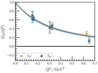
Figure 28: Quark-flavour contributions to ${G_{{E}}(Q^{2})}$ for the first positive-parity excitation at $m_{\pi}=$411\text{\,}\mathrm{MeV}$$. The curves are dipole fits to the form factor, with lines indicating the central values. The fits correspond to RMS charge radii of $0.871(36)\text{\,}\mathrm{fm}$ for the doubly represented quark flavour (${u_{{p^{\prime}}}}$) and $0.885(44)\text{\,}\mathrm{fm}$ for the singly represented quark flavour (${d_{{p^{\prime}}}}$).

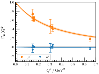
Figure 29: ${G_{{E}}(Q^{2})}$ for the first positive-parity excitations of the proton and neutron at $m_{\pi}=$411\text{\,}\mathrm{MeV}$$. The curves correspond to combinations of the quark-sector dipole fits from Fig. 28, giving a squared charge radius of $0.75(7)\text{\,}{\mathrm{fm}}^{2}$ for the proton and $0.016(39)\text{\,}{\mathrm{fm}}^{2}$ for the neutron.

V.1.2 Baryon electric form factors

As above, we take linear combinations of the individual quark flavour contributions, including the charges of the quark flavours and their multiplicity, to get the electric form factors for the first positive-parity excitations of the proton and neutron. In Fig. 29, we plot these combinations at $m_{\pi}=$411\text{\,}\mathrm{MeV}$$. At this and the other four masses, we find that the electric form factor for the neutron excitation is approximately zero.

In Fig. 30, we plot the pion-mass dependence of charge radii extracted from combinations of the quark-sector dipole fits to the electric form factor. For the heaviest three masses, squared charge radii for the proton range from $0.67(7)\text{\,}{\mathrm{fm}}^{2}$ to $0.75(7)\text{\,}{\mathrm{fm}}^{2}$, increasing with decreasing pion mass. These radii are all significantly larger than the charge radius of the ground-state proton at the corresponding mass. Thus the second positive-parity excitation is significantly larger than the ground state proton at these pion masses, in line with earlier observations that this positive parity excitation has a wave function consistent with a three-quark radial excitation with one node Roberts et al. (2013, 2014). At the lightest two masses, the statistical errors become large. However the trend for this positive parity excitation to be larger than the ground state is manifest.

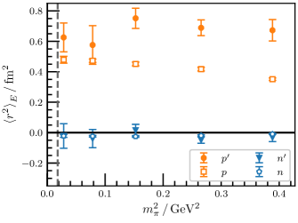
Figure 30: Quark-mass dependence of charge radii from combinations of quark-sector dipole fits to ${G_{{E}}(Q^{2})}$ for the first positive-parity excitation of the proton.

V.2 Magnetic form factor

V.2.1 Quark-flavour contributions

Having investigated the electric form factor for this state, we now consider the magnetic form factor. In Fig. 31 we plot the Euclidean sink-time dependence of the extracted form factors at $m_{\pi}=$702\text{\,}\mathrm{MeV}$$, with the lowest-momentum kinematics. We see that the form factors and plateaus for both analyses are very similar, and there is no evidence for opposite-parity contamination of this state. We see similar results for the other masses and kinematics, with no clear differences between the conventional and PEVA plateaus. For example, Fig. 32 shows this behaviour at $m_{\pi}=$411\text{\,}\mathrm{MeV}$$ with the same lowest-momentum kinematics. This suggests that, like ${G_{{E}}(Q^{2})}$, ${G_{{M}}(Q^{2})}$ for the first positive-parity excitation is not affected by opposite parity excitations, at least at this level of statistics.

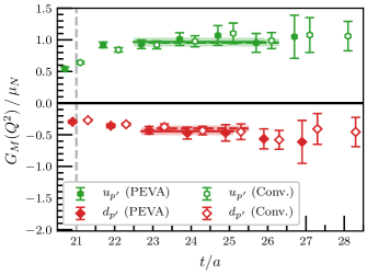
Figure 31: Quark-flavour contributions to the magnetic form factor for the first positive-parity excitation of the nucleon at $m_{\pi}=$702\text{\,}\mathrm{MeV}$$ for the lowest-momentum kinematics, providing $Q^{2}=$0.1425(41)\text{\,}\mathrm{G}\mathrm{eV}^{2}$$. Results are for single quarks of unit charge. All four fits start from time slice $23$ and have consistent values.

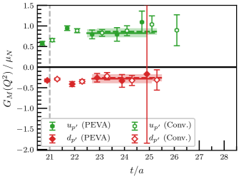
Figure 32: Quark-flavour contributions to ${G_{{M}}(Q^{2})}$ for the first positive-parity excitation of the nucleon at $m_{\pi}=$411\text{\,}\mathrm{MeV}$$ for the lowest-momentum kinematics, providing $Q^{2}=$0.146\text{\,}\mathrm{G}\mathrm{eV}^{2}$$.

Focusing on the PEVA results, we plot the $Q^{2}$ dependence of the plateau fits for the two valence quark flavours at $m_{\pi}=$411\text{\,}\mathrm{MeV}$$ in Fig. 33. We see that both quark flavours agree well with a dipole ansatz. This is also true for the two heavier pion masses, and the two lighter masses are also consistent, though they are too noisy to significantly constrain the fit.

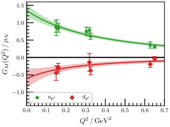
Figure 33: Quark-flavour contributions to ${G_{{M}}(Q^{2})}$ for the first positive-parity excitation at $m_{\pi}=$411\text{\,}\mathrm{MeV}$$. The curves are dipole fits to the form factor, corresponding to squared magnetic radii of $0.67(14)\text{\,}{\mathrm{fm}}^{2}$ for ${u_{{p^{\prime}}}}$ and $0.97(59)\text{\,}{\mathrm{fm}}^{2}$ for ${d_{{p^{\prime}}}}$.

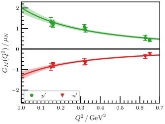
Figure 34: ${G_{{M}}(Q^{2})}$ for the first positive-parity excitations of the proton and neutron at $m_{\pi}=$411\text{\,}\mathrm{MeV}$$. The curves correspond to combinations of the quark-sector dipole fits from Fig. 33, giving a squared magnetic radius of $0.70(13)\text{\,}{\mathrm{fm}}^{2}$ for the proton excitation and $0.77(21)\text{\,}{\mathrm{fm}}^{2}$ for the neutron excitation.

V.2.2 Baryon magnetic form factors

Combinations of the quark flavour contributions are taken to form the proton and neutron excitations. In Fig. 34, we plot these combinations at $m_{\pi}=$411\text{\,}\mathrm{MeV}$$. By combining the dipole fits to the quark-sector results in the same way, we obtain magnetic radii that are consistent with the corresponding excited proton charge radius. This can be seen in Fig. 35, in which we plot the pion-mass dependence of the squared magnetic radii obtained from the linear combinations of the dipole fits to the form factors. These plots show fairly consistent results for the heavier three masses, with some pion-mass dependence. We omit results for the lightest two masses because the form factor data is insufficient to constrain dipole fits at these masses.

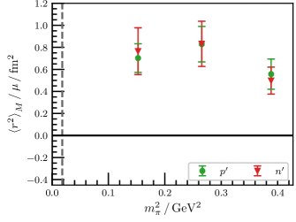
Figure 35: Quark-mass dependence of squared magnetic radii of the first positive-parity excitation of the proton and neutron from quark-sector dipole fits to ${G_{{M}}(Q^{2})}{}$. At the lightest two pion masses, the form factor data was insufficient to properly constrain a dipole fit so we do not report magnetic radii at these masses.

V.2.3 Baryon magnetic moments

Returning to the individual quark sector results and noting that once again the electric and magnetic form factors have a similar $Q^{2}$ dependence, we take the ratio ${\mu_{{\mathrm{{eff}}}}}{}(Q^{2})\equiv{G_{{M}}(Q^{2})}{}/{G_{{E}}(Q^{2})}{}$. In Fig. 36, we plot this ratio as a function of $Q^{2}$ for $m_{\pi}=$411\text{\,}\mathrm{MeV}$$. We find that the ratio is once again very flat in $Q^{2}$, supporting our hypothesis that the form factors have the same $Q^{2}$ scaling in this region, and the validity of ${\mu_{{\mathrm{{eff}}}}}{}$ as an estimate of the magnetic moment.

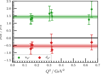
Figure 36: ${\mu_{{\mathrm{{eff}}}}}{}$ for individual quarks of unit charge in the first positive-parity excitation at $m_{\pi}=$411\text{\,}\mathrm{MeV}$$. The shaded bands are constant fits to the effective magnetic moments which provide magnetic moment contributions of $1.43(13)$ $\mu_{N}$ for the doubly represented quark and $-0.55(14)$ $\mu_{N}$ for the singly represented quark.

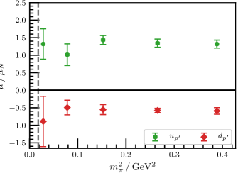
Figure 37: Quark-mass dependence of contributions from individual unit-charge quarks to the magnetic moment of the first positive-parity excitation of the nucleon. The vertical dashed line corresponds to the physical pion mass.

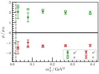
Figure 38: Quark-mass dependence of the magnetic moments of the first positive-parity excitations of the proton and neutron. The vertical dashed line corresponds to the physical pion mass, and the ground state magnetic moments have been plotted with open markers.

In Fig. 37, we plot the pion-mass dependence of ${\mu_{{\mathrm{{eff}}}}}{}$ for individual quarks of unit charge. We can once again take combinations of the individual quark-flavour contributions to get the excited proton and neutron magnetic moments. In Fig. 38, we plot the pion-mass dependence of these combinations.

We see that the excited-state magnetic moments agree well with the ground-state magnetic moments, particularly at the heaviest quark masses, where the agreement is impressive. These results are in accord with a simple $2S$ constituent-quark-model state.

In summary, we have shown that the first positive-parity excitation of the nucleon has no obvious opposite-parity contaminations. However, variational analysis techniques in general have provided good access to this state at several pion masses. This has allowed us to ascertain for the first time that these states have a larger radius than the ground-state nucleon, but have very similar magnetic moments. This is consistent with these states being dominated by a radial $2S$ excitation of the ground-state nucleon as seen in Refs. Roberts et al. (2013, 2014). Table 7, collects our charge radii, magnetic radii, and magnetic moments for this positive-parity excitation of the proton and neutron.

Table 7: Radii and magnetic moments of the positive-parity excitation of the proton and neutron. Radii are obtained from from combinations of quark-sector dipole fits and magnetic moments are obtained from quark-sector ratios of ${G_{{M}}(Q^{2})}$ to ${G_{{E}}(Q^{2})}{}$. At the lightest two pion masses, the form factor data was insufficient to properly constrain a dipole fit so we do not report magnetic radii at these masses.

$m_{\pi}^{2}\,/\,$\mathrm{G}\mathrm{eV}^{2}$$	${\braket{r^{2}}^{{p^{\prime}}}_{{E}}}{}\,/\,${\mathrm{fm}}^{2}$$	${\braket{r^{2}}^{{p^{\prime}}}_{{M}}}{}\,/\,{\mu^{{p^{\prime}}}}{}\!\,/\,${\mathrm{fm}}^{2}$$	${\mu^{{p^{\prime}}}}{}\!\,/\,\mu_{N}$
$0.3884$ p m 0.0113	$0.673$ p m 0.073	$0.56$ p m 0.14	$1.95$ p m 0.17
$0.2654$ p m 0.0081	$0.689$ p m 0.056	$0.83$ p m 0.16	$1.98$ p m 0.17
$0.1525$ p m 0.0043	$0.751$ p m 0.069	$0.70$ p m 0.13	$2.09$ p m 0.18
$0.0784$ p m 0.0025	$0.576$ p m 0.128	—	$1.52$ p m 0.44
$0.0285$ p m 0.0012	$0.626$ p m 0.097	—	$2.06$ p m 0.68

$m_{\pi}^{2}\,/\,$\mathrm{G}\mathrm{eV}^{2}$$	${\braket{r^{2}}^{{n^{\prime}}}_{{E}}}{}\,/\,${\mathrm{fm}}^{2}$$	${\braket{r^{2}}^{{n^{\prime}}}_{{M}}}{}\,/\,{\mu^{{n^{\prime}}}}{}\!\,/\,${\mathrm{fm}}^{2}$$	${\mu^{{n^{\prime}}}}{}\!\,/\,\mu_{N}$
$0.3884$ p m 0.0113	$-0.032$ p m 0.027	$0.50$ p m 0.12	$-1.27$ p m 0.11
$0.2654$ p m 0.0081	$-0.049$ p m 0.021	$0.83$ p m 0.21	$-1.28$ p m 0.10
$0.1525$ p m 0.0043	$0.016$ p m 0.039	$0.77$ p m 0.21	$-1.32$ p m 0.12
$0.0784$ p m 0.0025	$-0.039$ p m 0.060	—	$-1.00$ p m 0.29
$0.0285$ p m 0.0012	$-0.022$ p m 0.081	—	$-1.47$ p m 0.62

VI Conclusion

In this paper we presented the first calculations of the elastic form factors of lattice nucleon excitations from the first principles of QCD. We have considered a variety of momentum frames to access a range of $Q^{2}$ values, with some approaching zero. We have presented the first implementation of the PEVA technique for matrix elements, which is vital to isolating exited baryons with non-zero momentum.

Substantial differences between the form factors calculated in a conventional variational analysis and those calculated with the PEVA approach show the PEVA technique to be critical to understanding the structure of these excited states.

We find the size of the two lowest-lying negative parity excitations to be similar to the ground state nucleons. This is a remarkable result in the context of a simple constituent quark model, where the repulsive centripetal term of the radial Schrödinger equation proportional to $\ell\,(\ell+1)$ is expected to force the quarks to larger radii for $\ell=1$ states. The lattice QCD results point to a role for meson-nucleon Fock-space components in the $N^{*}$ states. As the antiquark in the meson provides the negative parity, all quarks can reside in relative $s$-waves. In this way the centripetal barrier is avoided and the negative-parity states can have a size similar to the ground state nucleon.

The positive-parity excitation observed in this study is very high in energy, approaching $2\text{\,}\mathrm{GeV}$, and exhibits challenging statistical fluctuations. The extractions of the form factors herein are attained through the cancellation of statistical fluctuations enabled by the combination of an ${\cal O}(a)$-improved conserved vector current and an appropriately selected correlator ratio preserving the lattice Ward identity. This state has a charge radius approximately $30\text{\,}\mathrm{\char 37\relax}$ larger than the ground state, and magnetic moments which match the ground state. Both of these observations are in accord with earlier observations that this positive parity excitation has a wave function consistent with a three-quark $2S$ radial excitation Roberts et al. (2013, 2014).

At the heaviest three pion masses considered, the first observed negative-parity excitations have magnetic moments consistent with quark-model descriptions for the $N^{*}(1535)$. Similarly, the second negative-parity excitations have magnetic moments in accord with quark-model descriptions of the $N^{*}(1650)$. At these quark masses, the results indicate these states are similar in structure to the ground state nucleon which can also be modelled as a three-quark state dressed by a meson cloud.

At the lightest two pion masses, we observe a rearrangement in the structure of the second negative-parity excitation. This is evident in both a significant shift in the magnetic moments of the excited proton and neutron, and significant curvature in the pion-mass dependence of the electric form factor. A description of this state as a molecular bound state of $K\Sigma$ dressed by $K\Lambda$, $\eta N$ and $\pi N$ is an intriguing possibility, analogous to the description of the odd-parity $\Lambda(1405)$ excitation as a molecular bound state of $\smash{\overline{K}}\vphantom{K}N$ dressed by $\pi\Sigma$ Hall et al. (2015, 2017). The proximity of the non-interacting $K\Sigma$ to the effective energy of the observed lattice state is suggestive.

While the current analysis is able to raise such a possibility, it is not able to affirm it. As a first step, non-local momentum-projected two-particle interpolating fields must be introduced to provide access to the $K\Sigma$, $K\Lambda$, $\eta N$ and $\pi N$ scattering states. To date, only the energy of the $S$-wave $\pi N$ scattering state has been investigated Lang and Verduci (2013); Liu et al. (2016). This will be a challenging endeavour, owing to the computational cost of estimating the loop propagators that are necessary to compute non-local momentum-projected meson-baryon contracted interpolating fields. Moreover, very high statistics will be required to precisely evaluate the correlation functions for quark masses near the physical regime.

However, such studies will allow for the lattice determination of the form factors of the multi-particle dominated scattering-states at light quark masses, and will provide the input required to make a robust connection between these states and the infinite-volume resonances of nature Briceño and Hansen (2016); Baroni et al. (2019).

Looking forward, it is interesting to note that HEFT calculations describe the negative-parity energy spectrum with reference to one bare basis state Liu et al. (2016). This investigation indicates the presence of two quark-model like states raising the possibility of introducing a second bare basis state into the formalism. It will be interesting to explore such an extension of HEFT as the two quark-model-like basis states mix through couplings to intermediate meson-baryon basis states. Such dynamics may be relevant to a detailed quantitative understanding of the negative-parity nucleon spectrum.

*