Solving Polynomial Systems with phcpy

Abstract

The solutions of a system of polynomials in several variables are often needed, e.g.: in the design of mechanical systems, and in phase-space analyses of nonlinear biological dynamics. Reliable, accurate, and comprehensive numerical solutions are available through PHCpack, a FOSS package for solving polynomial systems with homotopy continuation.

This paper explores new developments in phcpy, a scripting interface for PHCpack, over the past five years. For instance, phcpy is now available online through a JupyterHub server featuring Python2, Python3, and SageMath kernels. As small systems are solved in real-time by phcpy, they are suitable for interactive exploration through the notebook interface. Meanwhile, phcpy supports GPU parallelization, improving the speed and quality of solutions to much larger polynomial systems. From various model design and analysis problems in STEM, certain classes of polynomial system frequently arise, to which phcpy is well-suited.

1 Introduction

The Python package phcpy [Ver14] provides an alternative to the command line executable phc of PHCpack [Ver99] to solve polynomial systems by homotopy continuation methods. In the phcpy interface, Python scripts replace command line options and text menus, and data persists in a session without temporary files. This also makes PHCpack accessible from Jupyter notebooks, including a JupyterHub server available online [Pascal].

phcpy takes as input a list of polynomials in several variables, with complex-valued floating-point coefficients. Homotopy methods connect this given system to a ’start system’ with known solutions. A homotopy is a family of polynomial systems where one of the variables is considered as a parameter. Polynomial homotopy continuation combines the application of homotopy and continuation methods, which extend the convergence of Newton’s method from local to global, to solve polynomial systems.

Numerical continuation methods track the solution paths, depending on the parameter, originating at the known solutions to the solutions of the given system. phcpy is also able to represent the numerical irreducible decomposition of the system’s solution set, which yields the positive dimensional solution sets containing infinitely many points, in addition to the isolated solutions.

The focus of this paper is on the application of new technology to solve polynomial systems, in particular, cloud computing [BSVY15] and multicore shared memory parallelism accelerated with graphics processing units [VY15]. Our web interface offers phcpy in a SageMath [Sage], [SJ05] kernel or in a Python kernel of a Jupyter notebook [Klu16].

Although phcpy has been released for only five years, three instances in the research literature of symbolic computation, geometry and topology, and chemical engineering (respectively) mention its application to their computations.

• The number of embeddings of minimally rigid graphs [BELT18].

• Roots of Alexander polynomials [CD18].

• Critical points of equilibrium problems [SWM16].

The package phcpy is in ongoing development. At the time of writing, this paper is based on version 0.9.5 of phcpy, whereas version 0.1.5 was current at the time of [Ver14]. An example of these changes is that the software described in [SVW03] was recently parallelized for phcpy [Ver18].

1.1 A Scripting Interface for PHCpack

The mission of phcpy is to bring polynomial homotopy continuation into Python’s computational ecosystem.

The package phcpy wraps the shared object files of a compiled PHCpack, which makes the methods more accessible without sacrificing their efficiency. First, the wrapping transfers the implementation of the many available homotopy algorithms in a direct way into Python modules. Second, we do not sacrifice the efficiency of the compiled code. Scripts replace the input/output movements and interactions with the user, but not the computationally intensive algorithms.

Numerical algebraic geometry [SVW05] was introduced in 1995 as a pun on numerical linear algebra. PHCpack prototyped the first algorithms to compute a numerical irreducible decomposition of the solution set of a polynomial system. The package phcpy aims to bring the algorithms of numerical algebraic geometry into the computational ecosystem of Python.

1.2 Related Software

PHCpack is one of three FOSS packages for polynomial homotopy computation currently under development. Of these, only Bertini 2 [Bertini2.0] also offers Python bindings, although it is not GPU-accelerated and does not export the numerical irreducible decomposition, among other differences. Version 1.4 of Bertini is described in [BHSW13].

HomotopyContinuation.jl [HCJL] is a standalone package for Julia, presented at ICMS 2018 [BT18].

NAG4M2 [NAG4M2] is a package for Macaulay2 (a standard computational algebra system [M2]), which can also act an interface to PHCpack or Bertini. As described in [Ley11], it provided the starting point for PHCpack’s Macaulay2 bindings [GPV13].

2 User Interaction

2.1 Online Access

The first area of improvement that phcpy brings is in the interaction with the user.

With JupyterHub [JUPH], we provide online access [Pascal] to environments with Python and SageMath kernels pre-installed, both featuring phcpy and tutorials on its use (per next section). Since Jupyter is language-agnostic, execution environments in several dozen languages are possible. Our users can also run code in a Python Terminal session. As of the middle of May 2019, our web server has 146 user accounts, each having access to our JupyterHub instance. Our server is available for public use, after creating a free account.

In our first design of a web interface to phc, we developed a collection of Python scripts (mediated through HTML forms), following common programming patterns [Chu06]. This design is described in Chapter 6 of [Yu15]. For the user administration of our JupyterHub, we refreshed this first web interface, retaining the following architecture.

MySQLdb [MSDB] does the management of user data, including a) names and encrypted passwords, b) generic, random folder names to store data files, and c) file names with polynomial systems they have solved. With the module smtplib, we defined email exchanges for an automatic 2-step registration process and password recovery protocol.

A custom JupyterHub Authenticator connects to the existing MySQL database and triggers a SystemdSpawner that isolates the actions of users to separate processes and logins in generic home folders. The email account management prompts were hooked to new Tornado RequestHandler instances, which perform account registration and activation in the database, as well as password recovery and reset. Each such route serves HTML forms seamlessly with the JupyterHub interface, by extending its Jinja templates.

2.2 Code Snippets

Learning a new API is daunting enough without also being a crash course in algebraic geometry. Therefore, the user’s manual of phcpy [PHCPY] begins with a tutorial section using only the blackbox solver phcpy.solver.solve(system, ...). In this API, system is a list of strings representing polynomials, terminated by semicolons, and containing as many variables as equations.

The code snippets from these tutorials are available in our JupyterHub deployment, via the snippets menu provided by nbextensions [JUP15]. This menu suggests typical applications to guide the novice user. The screen shot in Fig. 1 shows the code snippet reproduced below.

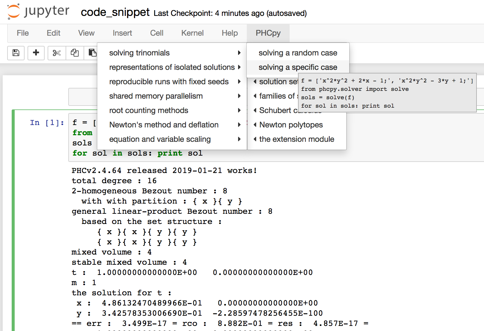
Figure 1: The code snippet for the blackbox solver.

   # PHCpy > blackbox solver > solving trinomials
   #       > solving a specific case
   from phcpy.solver import solve

   f = [’x^2*y^2 + 2*x - 1;’, ’x^2*y^2 - 3*y + 1;’]
   sols = solve(f)
   for sol in sols: print(sol)

The first solution of the given trinomial can be read as (0.48613… + 0.0i, 0.34258… - 0.0i), where the imaginary part of x is exactly zero, and that of y negligibly small. Programmatically, these can be accessed using either solve(f, dictionary_output=True), or equivalently by parsing strings through
[phcpy.solutions.strsol2dict(sol) for sol in solve(f)].

2.3 Direct Manipulation

One consequence of the Jupyter notebook’s rich output is the possibility of rich input, as explored through ipywidgets [IPYW] and interactive plotting libraries. The combination of rich input with fast numerical methods makes surprising interactions possible, such as interactive solution of Apollonius’ Problem, which is to construct all circles tangent to three given circles in a plane.

The tutorial given in the phcpy documentation was adapted for a demo accompanying a SciPy poster in 2017, whose code [APP] will run on our JupyterHub (by copying apollonius_d3.ipynb and apollonius_d3.js to one’s own user directory).

This system of 3 nonlinear constraints in 5 parameters for each of 8 possible tangent circles can be solved interactively by our system in real-time (Fig. 2). Although any of the 8 tangent circles could have nonzero imaginary part in their x/y position or radius, depending on input coefficients (input circles), such circles are not rendered. Thanks to its rich output capabilities, Jupyter is a suitable environment for mapping algebraic inputs to the planar geometric objects they represent (a data binding) through D3.js [D3].

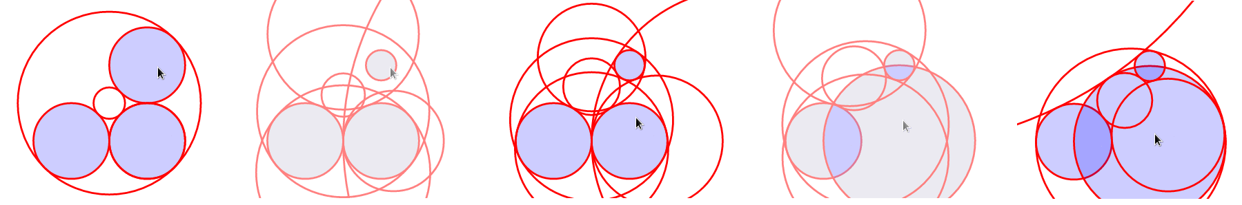
Figure 2: Tangent circles calculated by phcpy in response to user reparameterization of the system.

This approach makes use of the real-time solution of small polynomial systems, demonstrating the low latency of phcpy. It complements static input conditions by investigating their continous deformation, especially across singular solutions (which PHCpack handles more robustly than naive homotopy methods). Singular solutions of polynomial systems are handled by deflation [LVZ06], which restores quadratic convergence of Newton’s method by the addition of sufficiently many higher order derivatives to the original system.

3 Solving Polynomial Systems

Our input is a list of polynomials in several variables. This input list represents a polynomial system. By default, the coefficients of the polynomials are considered as complex floating point numbers. The system is then solved over the field of complex numbers.

For general polynomial systems, the complexity of the solution set can be expected to grow exponentially in the dimensions (number of polynomials and variables) of the system. The complexity of computing all solutions of a polynomial system is #P-hard. The complexity class #P is the class of counting problems. Formulating instances of polynomial systems that will occupy fast computers for a long time is not hard.

3.1 Polynomial Homotopy Continuation

By computing over the field of complex numbers, we exploit the continuity of the solution set as a function of the coefficients of the polynomials in the system. These numerical algorithms, called continuation methods, track solution paths defined by a one parameter family of polynomial systems (the homotopy). Homotopy methods take a polynomial system as input, and construct a suitable embedding of the input system into a family which contains a start system with known solutions.

We say that a homotopy is optimal if for generic instances of the coefficients of the input system no solution paths diverge. Even as the complexity of the solution set is very hard, the problem of computing the next solution, or just one random solution, has a much lower complexity. phcpy offers optimal homotopies for three classes of polynomial systems:

1. dense polynomial systems

   A polynomial of degree d can be deformed into a product of d linear polynomials. If we do this for all polynomials in the system (as in [VC93]), then the solutions of the deformed system are solutions of linear systems. Continuation methods track the paths originating at the solutions of the deformed system to the given problem.

2. sparse polynomial systems

   A system is sparse if relatively few monomials appear with nonzero coefficient. The convex hulls of the exponent vectors of the monomials that appear are called Newton polytopes. The mixed volume of the tuple of Newton polytopes associated with the system is a sharp upper bound for the number of isolated solutions. Polyhedral homotopies ([HS95], [VVC94]) start at solutions of systems that are sparser than the given system and extend those solutions to the solutions of the given problem.

3. Schubert problems in enumerative geometry

   The classical example is to compute all lines in 3-space that meet four given lines nontrivially. Homotopies to solve geometric problems move the input data to special position, solve the special configuration, and then deform the solutions of the special problem into those of the original problem. Such homotopies were introduced in [HSS98].

All classes of homotopies share the introduction of random constants.

For its fast mixed volume computation, the software incorporates MixedVol [GLW05] and DEMiCs [MT08]. High-precision double double and quad double arithmetic is performed by the algorithms in QDlib [HLB01].

3.2 Speedup and Quality Up

The solution paths defined by polynomial homotopies can be tracked independently, providing obvious opportunities for parallel execution. This section reports on computations on our server, a 44-core computer.

An obvious benefit of running on many cores is the speedup. The quality up question asks the following: if we can afford to spend the same time, by how much can we improve the solution using p processors?

We illustrate the quality up question on the cyclic 7-roots benchmark problem [BF91]. The online SymPy documentation [SymPyDocs] uses the cyclic 4-roots problem to illustrate its nonlinsolve method.

The function defined below returns the elapsed performance of the blackbox solver on the cyclic 7-roots benchmark problem, for a number of tasks and a precision equal to double, double double, or quad double arithmetic.

    def qualityup(nbtasks=0, precflag=’d’):
        """
        Runs the blackbox solver on a system.
        The default uses no tasks and no multiprecision.
        The elapsed performance is returned.
        """
        from phcpy.families import cyclic
        from phcpy.solver import solve
        from time import perf_counter
        c7 = cyclic(7)
        tstart = perf_counter()
        s = solve(c7, verbose=False, tasks=nbtasks, \
                  precision=precflag, checkin=False)
        return perf_counter() - tstart

The function above is applied in an interactive Python script, prompting the user for the number of tasks and precision, This scripts runs in a Terminal window and prints the elapsed performance returned by the function. If the quality of the solutions is defined as the working precision, then to answer the quality up question, one considers how many processors are needed to compensate for the overhead of the multiprecision arithmetic.

Although cyclic 7-roots is a small system for modern computers, the cost of tracking all solution paths in double double and quad double arithmetic causes significant overhead. The script above was executed on a 2.2 GHz Intel Xeon E5-2699 processor in a CentOS Linux workstation with 256 GB RAM and the elapsed performance is in Table 1.

precision	d	dd	qd
elapsed performance	5.45	42.41	604.91
overhead factor	1.00	7.41	110.99

Table 1: Elapsed performance of the blackbox solver in double, double double, and quad double precision.

Table 2 demonstrates the reduction of the overhead caused by the multiprecision arithmetic by multitasking.

tasks	8	16	32
dd	7.56	5.07	3.88
qd	96.08	65.82	44.35

Table 2: Elapsed performance of the blackbox solver with 8, 16, and 32 path tracking tasks, in double double and quad double precision.

Notice that the 5.07 in Table 2 is less than the 5.45 of Table 1: with 16 tasks we doubled the precision and finished the computations in about the same time. The 42.41 and 44.35 in Table 2 are similar enough to state that with 32 instead of 1 task we doubled the precision from double double to quad double precision in about the same time.

The data in Table 2 is visualized in Fig. 3. The interpolation allows us to estimate running times for a number of tasks different from the measured run times. To answer the original quality up question, one could interpolate between the sizes of working precision to answer the following quality up question. If we can afford to spend the same time as on one path tracking task, then how many extra decimal places can we gain with p path tracking tasks?

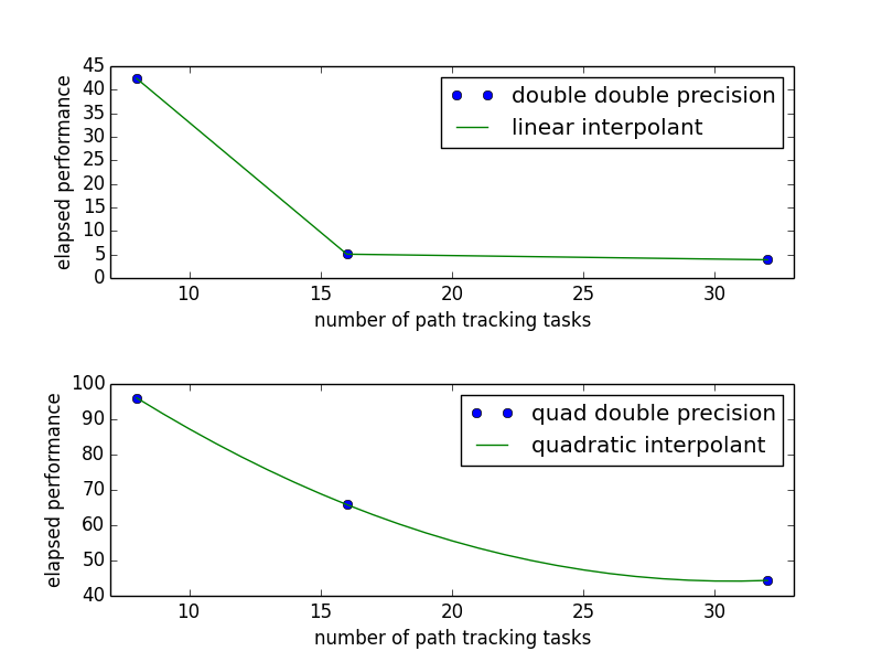
Figure 3: Interpolated elapsed performances.

Precision is a crude measure of quality. Another motivation for quality up by parallelism is to compensate for the cost overhead caused by arithmetic with power series. Power series are hybrid symbolic-numeric representations for algebraic curves.

3.3 Positive Dimensional Solution Sets

Solving a system has evolved in meaning, from computing approximations of all its isolated solutions, to finding the numerical irreducible decomposition of the solution set. The numerical irreducible decomposition includes not only the isolated solutions, but also the representations for all positive dimensional solution sets. Such representations consist of sets of generic points, partitioned along the irreducible factors.

To illustrate this expanded sense of a ’solution’, we consider the twisted cubic, known in algebraic geometry as the first nontrivial space curve. We use this example to illustrate two different representations of this space curve:

1. In a witness set construction, the given polynomial equations are augmented with as many generic hyperplanes as the dimension of the solution set. The solutions which satisfy the system and the augmented equations are generic points. As the degree of the twisted cubic is three, we find three points on a random plane intersecting the cubic.

         pols = [’x*y - z;’, ’x^2 - y;’]
         from phcpy.sets import embed
         from phcpy.solver import solve
         embp = embed(3, 1, pols)
         sols = solve(embp, verbose=False)
         print(’#generic points :’, len(sols))
   

   The above snippet constructs the embedding for the equations that define the twisted cubic. The solutions of this embedding represent the curve. Moving the added plane and tracking the solution paths starting at the three generic points will provide many more samples of the curve.

2. A series expansion for the solution starts its development at some point(s) in a coordinate hyperplane. In this hyperplane, the curve intersects the solution set at some point(s). For a simple example as the twisted cubic, the series development defines an exact solution after the initial term. Consider the snippet:

         pols = [’x*y - z;’, ’x^2 - y;’]
         from phcpy.maps import solve_binomials
         maps = solve_binomials(3, pols, \
                    puretopdim=True)
         for sol in maps:
             print(sol)
   

   The output of the above snippet is

         [’x - (1+0j)*t1**1’, ’y - (1+0j)*t1**2’, \
          ’z - (1+0j)*t1**3’, ’dimension = 1’, \
          ’degree = 3’]
   

   which corresponds to the parametric respresentation $(t,t^{2},t^{3})$ of the twisted cubic.

Many interesting polynomial systems have isolated solutions and positive dimensional solution sets. We consider again the family of cyclic n-roots problems, now for $n=8$, [BF94]. While for $n=7$ all roots are isolated points, there is a one dimensional solution curve of cyclic 8-roots of degree 144. This curve decomposes in 16 irreducible factors, eight factors of degree 16 and eight quadratic factors, adding up to $8\times 16+8\times 2=144$.

Consider the following code snippet.

    from phcpy.phcpy2c3 import py2c_set_seed
    from phcpy.factor import solve
    from phcpy.families import cyclic
    py2c_set_seed(201905091)  # for a reproducible run
    c8 = cyclic(8)
    sols = solve(8, 1, c8, verbose=False)
    witpols, witsols, factors = sols[1]
    deg = len(witsols)
    print(’degree of solution set at dimension 1 :’, deg)
    print(’number of factors : ’, len(factors))
    _, isosols = sols[0]
    print(’number of isolated solutions :’, len(isosols))

The output of the script is

    degree of solution set at dimension 1 : 144
    number of factors :  16
    number of isolated solutions : 1152

This numerical output is the essence of the blackbox solver for positive dimensional solution sets [Ver18].

4 Survey of Applications

We consider some examples from various literatures which apply polynomial constraint solving. The first two examples use phcpy in particular as a research tool. The remaining three are broader examples representing current uses of numerical algebraic geometry in other STEM fields.

4.1 Rigid Graph Theory

The conformations of proteins [LML14], molecules [EM99], and robotic mechanisms (discussed further below) can be studied by counting and classifying unique mechanisms, i.e. real embeddings of graphs with fixed edge lengths, modulo rigid motions, per Bartzos et al. [BELT18].

Consider a graph $G$ whose edges $e\in E_{G}$ each have a given length $d_{e}$. A graph embedding is a function that maps the vertices of $G$ into $D$-dimensional Euclidean space (especially $D$ = 2 or 3). Embeddings which are ’compatible’ are those which preserve $G$’s edge lengths. The number of unique mechanisms is thus a function of $G$ and $\mathbf{d}$. An upper bound over all $d$ and $G$ with k vertices (yielding lower bounds for graphs with $n\geq k$ vertices, unless the upper bound is infinite) can be computed. In particular, the Cayley-Menger matrix of $\mathbf{d}$ [LLMM14] (i.e., the squared distance matrix with a row and column of 1s prepended, except that its main diagonal is 0s) is an algebraic system, proportional to the mixed volume. Certain of its square subsystems characterize the mechanism in terms of these bounds on unique mechanisms.

Bartzos et al. implemented, using phcpy, a constructive method yielding all 7-vertex minimally rigid graphs in 3D space (the smallest open case) and certain 8-vertex cases previously uncounted. A graph $G$ is generically rigid if, for any given edge lengths $d$, none of its compatible embeddings (into a generic configuration such that vertices are algebraically independent) are continuously deformable. $G$ is minimally rigid if removing any one of its edges yields a non-rigid mechanism.

phcpy was used to find edge lengths with maximally many real embeddings, exploiting the flexibility of being able to specify their starting system. This sped up their algorithm by perturbing the solutions of previous systems to find new ones.

Many iterations of sampling have to be performed if the wrong number of real embeddings is found; in each case, a different subgraph is selected based on a heuristic implemented by the DBSCAN class of scikit-learn (illustrating the value of a scientific Python ecosystem). The actual number of real embeddings is known from an enumeration of unique graphs constructed by Henneberg steps in, for instance, SageMath.

4.2 Model Selection & Parameter Inference

It is often useful to know all the steady states of a biological network, as represented by a nonlinear system of ordinary differential equations, with some conserved quantities. These two lists of polynomials (from rates of change of form $\dot{x}=p(x)$, by letting $\dot{x}=0$; and from conservation laws of form $c=\sum{x_{i}}$ by subtracting $c$ from both sides) have a zero set which is a steady-state variety, that can be explored numerically via polynomial homotopy continuation.

Parameter homotopies were used by Gross et al. [GHR16] to perform model selection on a mammalian phosphorylation pathway, determining whether the kinase acts processively (i.e. adding more than one phosphate at once, which it does not in vitro). Their analysis validated experimental work showing processivity in vivo. In doing so, they obtained ¿50x speedup over non-parameter homotopies (for running times in minutes, not hours) on systems tracking 20 paths.

4.3 Critical Point Computation

Polynomial homotopy continuation has also been adapted to the field of chemical engineering to locate critical points of multicomponent mixtures [SWM16], i.e., temperature and pressure satisfying a multi-phase equilibrium.

A remarkable variety of systems of constraint also take on polynomial form, or can be approximated thereby, in various sciences. Diverse problems in the analysis of belief propagation (in graphical models) [KMC18], hyperbolic conservation laws (in PDEs) [HHS13], and vacuum moduli spaces (in supersymmetric field theory) [HHM13] have been addressed using polynomial homotopy continuation.

4.4 Algebraic Kinematics

We have discussed an application of numerical methods to count ing unique instances of rigid-body mechanisms. In fact, kinematics and numerical algebraic geometry have a close historical relationship. Following Wampler and Sommese [WS11], other geometric problems arising from robotics include analysis of specific mechanisms e.g.,:

• Motion decomposition - into assembly modes (of individual mechanisms) or subfamilies of mechanisms (with varying mobility);

• Mobility analysis - degrees of freedom of a mechanism (sometimes exceptional), sometimes specific to certain configurations (e.g., gimbal lock);

• Kinematics - effector position given parameters (forward kinematics), and vice versa (inverse kinematics, e.g. used in computer animation);

• Singularity analysis - detection of situations where the mechanism can move without change to its parameters (input singularity), or the parameters can change without movement of the mechanism (output singularity);

• Workspace analysis - determining all possible outputs of the mechanism, i.e.: reachable poses;

…as well as the synthesis of mechanisms that can reach certain sets of outputs, or that can be controlled by a certain input/output relationship.

Fig. 4 illustrates a reproduction of one synthesis result in the mechanism design literature [MW90]. Given five points, the problem is to determine the length of two bars so their coupler curve passes through the five given points.

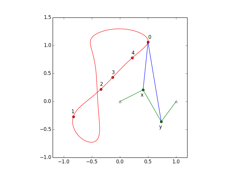
Figure 4: The design of a 4-bar mechanism.

This example is part of the tutorial of phcpy and the scripts to reproduce the results are in its source code distribution. The equations are generated with sympy [SymPy] and the plots are made with matplotlib [Hun07].

Continuation homotopies were developed as a substitute for algebraic elimination that was more robust to special cases, yet still tractable to numerical techniques. Research in kinematics increasingly relies on such algorithms [WS11].

4.5 Systems Biology

Whether a model biological system is multistationary or oscillatory, and whether this depends on its rate constants, are all properties of its steady-state locus. Following the survey of Gross et al. [GBH16] regarding uses of numerical algebraic geometry in this domain, one might seek to:

• determine which values of the rate and conserved-quantity parameters allow the model to have multiple steady states;

• evaluate models with partial data (subsets of the $x_{i}$) and reject those which don’t agree with the data at steady state;

• describe all the states accessible from a given state of the model, i.e. that state’s stoichiometric compatibility class (or basin of attraction);

• determine whether rate parameters of the given model are identifiable from concentration measurements, or at least constrained.

For large real-world models in systems biology, these questions of algebraic geometry are only tractable to numerical methods scaling to many dozens of simultaneous equations.

5 Conclusion

From these examples, we see that polynomial homotopy continuation has wide applicability to STEM fields. Moreover, phcpy is an accessible interface to the technique, capable of high performance whilst producing certifiable and reproducible results.

5.1 Acknowledgments

This material is based upon work supported by the National Science Foundation under Grant No. 1440534.

References

- [BHSW13] D. J. Bates, J. D. Hauenstein, A. J. Sommese, and C. W. Wampler. Numerically solving polynomial systems with Bertini, volume 25 of Software, Environments, and Tools, SIAM, 2013.
- [BELT18] E. Bartzos, I. Z. Emiris, J. Legersky, and E. Tsigaridas. On the maximal number of real embeddings of spatial minimally rigid graphs. In the Proceedings of the 2018 International Symposium on Symbolic and Algebraic Computation (ISSAC 2018), pages 55-62, ACM 2018. DOI 10.1145/3208976.3208994.
- [Bertini2.0] Bertini 2.0: The redevelopment of Bertini in C++. https://github.com/bertiniteam/b2
- [BF91] J. Backelin and R. Fröberg. How we proved that there are exactly 924 cyclic 7-roots. In the Proceedings of the 1991 International Symposium on Symbolic and Algebraic Computation (ISSAC’91), pages 103-111, ACM, 1991. DOI 10.1145/120694.120708.
- [BF94] G. Björck and R. Fröberg. Methods to “divide out” certain solutions from systems of algebraic equations, applied to find all cyclic 8-roots. In Analysis, Algebra and Computers in Mathematical Research, Proceedings of the twenty-first Nordic congress of mathematicians, edited by M. Gyllenberg and L. E. Persson, volume 564 of Lecture Notes in Pure and Applied Mathematics, pages 57-70. Dekker, 1994.
- [BSVY15] N. Bliss, J. Sommars, J. Verschelde, X. Yu. Solving polynomial systems in the cloud with polynomial homotopy continuation. In the Proceedings of the 17th International Workshop on Computer Algebra in Scientific Computing (CASC 2015), edited by V. P. Gerdt, W. Koepf, W. M. Seiler, and E. V. Vorozhtsov, volume 9301 of Lecture Notes in Computer Science, pages 87-100, Springer-Verlag, 2015. DOI 10.1007/978-3-319-24021-3_7.
- [D3] M. Bostock, V. Ogievetsky, and J. Heer D3 Data-Driven Documents. IEEE Transactions on Visualization and Computer Graphics, 17, pages 2301–2309, 2011. DOI 10.1109/TVCG.2011.185.
- [BT18] P. Breiding and S. Timme. HomotopyContinuation.jl: A package for homotopy continuation in Julia. In the proceedings of ICMS 2018, the 6th International Conference on Mathematical Software, South Bend, IN, USA, July 24-27, 2018, edited by J. H. Davenport, M. Kauers, G. Labahn, and J. Urban, volume 10931 of Lecture Notes in Computer Science, pages 458-465. Springer-Verlag, 2018. DOI 10.1007/978-3-319-96418-8.
- [Chu06] W. J. Chun. Core Python Programming. Prentice Hall, 2nd Edition, 2006.
- [CD18] M. Culler and N. M. Dunfield. Orderability and Dehn filling. Geometry and Topology, 22: 1405-1457, 2018. DOI 10.2140/gt.2018.22.1405.
- [EM99] I.Z. Emiris and B. Mourrain. Computer algebra methods for studying and computing molecular conformations. Algorithmica 25, pages 372–402, 1999. DOI: 10.1007/PL00008283.
- [APP] explorable circle tangency https://github.com/JazzTap/mcs563/tree/master/Apollonius]
- [HHM13] J. Hauenstein, Y.-H. He, and D. Mehta. Numerical elimination and moduli space of vacua. Journal of High Energy Physics, 83. 2013. DOI: 10.1007/JHEP09(2013)083.
- [HHS13] W. Hao, J. D. Hauenstein, C.-W. Shu, A. J. Sommese, Z. Xu, and Y.-T. Zhang. A homotopy method based on WENO schemes for solving steady state problems of hyperbolic conservation laws. Journal of Computational Physics, 250, pages 332–346. 2013. DOI: 10.1016/j.jcp.2013.05.008.
- [HLB01] Y. Hida, X. S. Li, and D. H. Bailey. Algorithms for quad-double precision floating point arithmetic. In the Proceedings of the 15th IEEE Symposium on Computer Arithmetic (Arith-15 2001), pages 155–162. IEEE Computer Society, 2001. DOI 10.1109/ARITH.2001.930115.
- [HCJL] A Julia package for solving systems of polynomials via homotopy continuation. https://github.com/JuliaHomotopyContinuation
- [Hun07] J. D. Hunter. Matplotlib: A 2D Graphics Environment. Computing in Science and Engineering 9(3): 90-95, 2007. DOI 10.1109/MCSE.2007.55.
- [GLW05] T. Gao, T.Y. Li, and M. Wu. Algorithm 846: MixedVol: a software package for mixed-volume computation. ACM Trans. Math. Softw., 31(4):555-560, 2005. DOI 10.1145/1114268.1114274.
- [GBH16] E. Gross, D. Brent, K. L. Ho, D. J. Bates, and H. A. Harrington. Numerical algebraic geometry for model selection and its application to the life sciences. Journal of The Royal Society Interface, 13: 20160256. 2016. DOI: 10.1098/rsif.2016.0256.
- [GHR16] E. Gross, H. A. Harrington, Z. Rosen, and B. Sturmfels. Algebraic Systems Biology: A Case Study for the Wnt Pathway. Bulletin of Mathematical Biology 78, pages 21–51, 2016. DOI: 10.1007/s11538-015-0125-1.
- [GPV13] E. Gross, S. Petrović, and J. Verschelde. Interfacing with PHCpack. The Journal of Software for Algebra and Geometry: Macaulay2, 5:20-25, 2013. DOI 10.2140/jsag.2013.5.20.
- [HS95] B. Huber and B. Sturmfels. A polyhedral method for solving sparse polynomial systems. Mathematics of Computation, 64(212):1541-1555, 1995. DOI 10.1090/S0025-5718-1995-1297471-4.
- [HSS98] B. Huber, F. Sottile, and B. Sturmfels. Numerical Schubert calculus. Journal of Symbolic Computation, 26(6):767-788, 1998. DOI 10.1006/jsco.1998.0239.
- [IPYW] ipywidgets: Interactive HTML Widgets https://github.com/jupyter-widgets/ipywidgets
- [SymPy] D. Joyner, O. Čertík, A. Meurer, and B. E. Granger. Open source computer algebra systems: SymPy. ACM Communications in Computer Algebra 45(4): 225-234 , 2011. DOI 10.1145/2110170.2110185.
- [Pascal] JupyterHub deployment of phcpy. Website, accessed May 2019. 2017. https://phcpack.org
- [JUPH] JupyterHub 0.7.2 documentation https://jupyterhub.readthedocs.io/en/0.7.2/index.html
- [JUP15] Jupyter notebook snippets menu - jupyter-contrib-nbextensions 0.5.0 https://jupyter-contrib-nbextensions.readthedocs.io/en/latest/nbextensions/snippets_menu/readme.html.
- [Klu16] T. Kluyver, B. Ragan-Kelley, F. Pérez, B. Granger, M. Bussonnier, J. Frederic, K. Kelley, J. Hamrick, J. Grout, S. Corlay, P. Ivanov, D. Avila, S. Abdalla, C. Willing, and Jupyter Development Team. Jupyter Notebooks – a publishing format for reproducible computational workflows. In Positioning and Power in Academic Publishing: Players, Agents, and Agendas, edited by F. Loizides and B. Schmidt, pages 87-90. IOS Press, 2016. DOI 10.3233/978-1-61499-649-1-87.
- [KMC18] C. Knoll, D. Mehta, T. Chen, and F. Pernkopf. Fixed Points of Belief Propagation—An Analysis via Polynomial Homotopy Continuation. IEEE Transactions on Pattern Analysis and Machine Intelligence, 40, pages 2124–2136, 2018. DOI 10.1109/TPAMI.2017.2749575.
- [Ley11] A. Leykin. Numerical algebraic geometry. The Journal of Software for Algebra and Geometry: Macaulay2, 3:5-10, 2011. DOI 10.2140/jsag.2011.3.5.
- [LVZ06] A. Leykin, J. Verschelde, and A. Zhao. Newton’s method with deflation for isolated singularities of polynomial systems. Theoretical Computer Science, 359(1-3):111-122, 2006. DOI 10.1016/j.tcs.2006.02.018.
- [LLMM14] L. Liberti, C. Lavor, N. Maculan, and A. Mucherino. Euclidean Distance Geometry and Applications. SIAM Review 56, no. 1 (January 2014): 3–69. DOI 10.1137/120875909
- [LML14] L. Liberti, B. Masson, J. Lee, C. Lavor, and A. Mucherino. On the number of realizations of certain henneberg graphs arising in protein conformation. Discrete Applied Mathematics, 165, page 213–232, 2014. DOI: 10.1016/j.dam.2013.01.020.
- [M2] D. R. Grayson and M. E. Stillman. Macaulay2, a software system for research in algebraic geometry. http://www.math.uiuc.edu/Macaulay2
- [MT08] T. Mizutani and A. Takeda. DEMiCs: A software package for computing the mixed volume via dynamic enumeration of all mixed cells. In Software for Algebraic Geometry, edited by M. E. Stillman, N. Takayama, and J. Verschelde, volume 148 of The IMA Volumes in Mathematics and its Applications, pages 59-79. Springer-Verlag, 2008. DOI 10.1007/978-0-387-78133-4.
- [MW90] A. P. Morgan and C. W. Wampler. Solving a Planar Four-Bar Design Using Continuation. Journal of Mechanical Design, 112(4): 544-550, 1990. DOI 10.1115/1.2912644.
- [NAG4M2] Branch NAG of M2 repository. https://github.com/antonleykin/M2/tree/NAG
- [MSDB] MySQLdb 1.2.4b4 documentation https://mysqlclient.readthedocs.io/
- [PHCPY] phcpy 0.9.5 documentation http://homepages.math.uic.edu/~jan/phcpy_doc_html/
- [Sage] The Sage Developers. SageMath, the Sage Mathematics Software System, Version 7.6. https://www.sagemath.org, 2016. DOI 10.5281/zenodo.820864.
- [SJ05] W. Stein and D. Joyner. Sage: System for algebra and geometry experimentation. ACM SIGSAM Bulletin 39(2): 61-64, 2005. DOI 10.1145/1101884.1101889.
- [SWM16] H. Sidky, J. K. Whitmer, and D. Mehta. Reliable mixture critical point computation using polynomial homotopy continuation. AIChE Journal. Thermodynamics and Molecular-Scale Phenomena, 62(12): 4497-4507, 2016. DOI 10.1002/aic.15319.
- [SVW03] A. J. Sommese, J. Verschelde, and C. W. Wampler. Numerical irreducible decomposition using PHCpack. In Algebra, Geometry and Software Systems, edited by M. Joswig and N. Takayama, pages 109-130, Springer-Verlag 2003. DOI 10.1007/978-3-662-05148-1_6.
- [SVW05] A. J. Sommese, J. Verschelde, and C. W. Wampler. Introduction to numerical algebraic geometry. In Solving Polynomial Equations, Foundations, Algorithms, and Applications, edited by A. Dickenstein and I. Z. Emiris, pages 301-337, Springer-Verlag 2005. DOI 10.1007/3-540-27357-3_8.
- [SymPyDocs] SymPy 1.3 documentation. https://docs.sympy.org/latest/index.html
- [Ver99] J. Verschelde. Algorithm 795: PHCpack: A general-purpose solver for polynomial systems by homotopy continuation, ACM Trans. Math. Softw., 25(2):251-276, 1999. DOI 10.1145/317275.317286.
- [Ver14] J. Verschelde. Modernizing PHCpack through phcpy. Proceedings of the 6th European Conference on Python in Science (EuroSciPy 2013), edited by P. de Buyl and N. Varoquaux, pages 71-76, 2014.
- [Ver18] J. Verschelde. A Blackbox Polynomial System Solver for Shared Memory Parallel Computers. In Computer Algebra in Scientific Computing, 20th International Workshop, CASC 2018, Lille, France, edited by V. P. Gerdt, W. Koepf, W. M. Seiler, and E. V. Vorozhtsov, volume 11077 of Lecture Notes in Computer Science, pages 361-375. Springer-Verlag, 2018. DOI 10.1007/978-3-319-99639-4_25.
- [VC93] J. Verschelde and R. Cools. Symbolic homotopy construction. Applicable Algebra in Engineering, Communication and Computing, 4(3):169-183, 1993. DOI 10.1007/BF01202036.
- [VVC94] J. Verschelde, P. Verlinden, and R. Cools. Homotopies exploiting Newton polytopes for solving sparse polynomial systems. SIAM Journal on Numerical Analysis 31(3):915-930, 1994. DOI 10.1137/0731049.
- [VY15] J. Verschelde and X. Yu. Polynomial Homotopy Continuation on GPUs. ACM Communications in Computer Algebra, volume 49, issue 4, pages 130-133, 2015. DOI 10.1145/2893803.2893810.
- [WS11] C. W. Wampler & A. J. Sommese Numerical algebraic geometry and algebraic kinematics. Acta Numerica, 20, pages 469–567. 2011. DOI: 10.1017/S0962492911000067.
- [Yu15] X. Yu. Accelerating Polynomial Homotopy Continuation on Graphics Processing Units. PhD thesis, University of Illinois at Chicago, 2015.