Dark matter heating of gas accreting onto Sgr A^∗

Abstract

We study effects of heating by dark matter (DM) annihilation on black hole gas accretion. We observe that, for reasonable assumptions about DM densities in spikes around supermassive black holes, as well as DM masses and annihilation cross-sections within the standard WIMP model, heating by DM annihilation may have an appreciable effect on the accretion onto Sgr A^∗ in the Galactic center. Motivated by this observation we study the effects of such heating on Bondi accretion, i.e. spherically symmetric, steady-state Newtonian accretion onto a black hole. We consider different adiabatic indices for the gas, and different power-law exponents for the DM density profile. We find that typical transonic solutions with heating have a significantly reduced accretion rate. However, for many plausible parameters, transonic solutions do not exist, suggesting a breakdown of the underlying assumptions of steady-state Bondi accretion. Our findings indicate that heating by DM annihilation may play an important role in the accretion onto supermassive black holes at the center of galaxies, and may help explain the low accretion rate observed for Sgr A^∗.

1 Introduction

The spectacular images recently provided by the Event Horizon Telescope (EHT) Collaboration (see Event Horizon Telescope Collaboration: K. Akiyama et.al., 2019, as well as several follow-up publications) have driven interest in accretion onto supermassive black holes to new heights. One of the targets of the EHT is Sgr A^∗, the supermassive black hole with mass $M=4\times 10^{6}M_{\odot}$ (Ghez et al., 2008; Genzel et al., 2010; Gillessen et al., 2017) residing at the Galactic center (GC). In this paper we are interested in the remarkably low rate at which gas in the central bulge is actually accreting onto Sgr A^∗: it has long been recognized that this rate, estimated to be a few times $\sim 10^{-8}M_{\odot}~{}{\rm yr}^{-1}$, is roughly three orders of magnitude below the standard Bondi estimate for the rate at which gas is gravitationally captured by the hole at $~{}0.1$ pc (Baganoff et al., 2003; Shcherbakov & Baganoff, 2010; Ressler et al., 2017). The Bondi value for the rate is determined from the gas density and temperature inferred from the diffuse X-ray emission observed by Chandra at $\sim 2$ arc sec ( $\sim 0.1$ pc) from the black hole and is $\sim 2\times 10^{-5}M_{\odot}~{}{\rm yr}^{-1}$. The rate at which gas actually accretes onto the black hole is inferred from polarization measurements (Marrone et al., 2007) and models of the near-horizon accretion flow and emitted luminosity (Shcherbakov & Baganoff, 2010; Ressler et al., 2017).

The current explanation for this large difference begins with the assumption that the gas originates from stellar winds from the $\sim 30$ Wolf-Rayet (WR) stars that orbit within $\sim 1$ pc from Sgr A^∗ and that this gas thus has a broad distribution of angular momentum. Hydrodynamic simulations in 3D (see, e.g. Cuadra et al., 2008; Ressler et al., 2018) then suggest that, while the inflow rate at $\sim 0.1$ pc is $\sim 2-3\times 10^{-5}M_{\odot}~{}{\rm yr}^{-1}$, which is close to the Bondi value for the rate at which gas is gravitationally bound to the black hole, only a small fraction of this mass actually accretes to smaller radii $\ll 0.1$ pc, since only the low angular momentum tail of the stellar wind is able to accrete. As it approaches the event horizon of Sgr A^∗, even this gas likely has sufficient angular momentum to form a geometrically thick disk. This near-horizon disk has been simulated in general relativistic radiation-magnetohydrodynamics by several investigators in recent years (see, e.g. Sa̧dowski et al., 2017; Ryan et al., 2017; Chael et al., 2018, and references therein), forming the theoretical framework for interpreting present and future observations of Sgr A^∗ by various instruments, including the EHT.

In this paper we investigate the possibility that heating by dark matter (DM) annihilation may provide another reason why the accretion rate onto Sgr A^∗ is much lower than the canonical Bondi value. We will explore this possibility by reconsidering the classic, steady-state, spherical Bondi flow problem (Bondi, 1952) but with heating arising from the inclusion of DM annihilation (see also Johnson & Quataert, 2007, who found that the inclusion of thermal conduction in the Bondi solution similarly leads to a reduction in the accretion rate). Among the parameters we allow to vary are the gas adiabatic index $\gamma$ and the DM density profile parameter $\alpha$. The choice of $\gamma$ roughly accounts for cooling, which is not incorporated explicitly in our equations: in the absence of heating, $\gamma=5/3$ applies to adiabatic flow (no cooling), while $\gamma=1$ applies to isothermal flow (extreme cooling). The parameter $\alpha$ is determined by the power-law that describes the increase in the DM density with decreasing radius $r$ from the GC.

Our goal is to use this simple, modified Bondi accretion model to determine whether such heating can suppress the inflow rate for a given set of gas dynamic parameters at large distance from the black hole and a physically plausible DM annihilation rate. Even if effective in reducing the accretion rate, it is not likely that spherical Bondi flow will supplant our current understanding of the more complicated flow patterns found in the 3D hydrodynamic simulations. However, if effective in the case of Bondi flow, heating by DM annihilation may be another mechanism that should be incorporated in future hydrodynamic simulations. (In “hot accretion" disk models like ADAFs, which also have been employed to model Sag A*, heating by viscous dissipation plays a dominant role; see, e.g., Yuan & Narayan (2014) for a review.)

This paper is organized as follows. Section 2 assembles plausible DM local and global parameters and uses them to construct the heating rate due to DM annihilation. Section 3 derives the basic Newtonian equations for steady-state, spherical accretion of gas from rest at infinity, incorporating this heating term. Section 4 identifies the range of parameters for which the flow smoothly crosses a transonic point and summarizes the accretion rates for such cases. Section 5 does the same for solutions that remain subsonic. Section 6 applies the results to the GC and Sgr A^∗. We summarize our findings in Section 7, and also delineate some caveats that might alter the results obtained in the earlier sections.

2 Heating rate due to DM annihilation

We adopt the standard weakly interacting massive particle (WIMP) model for the DM, which we treat as collisionless particles of mass $m_{\chi}$ that undergo annihilation reactions in a density spike around Sgr A^∗. The heating rate per unit volume due to annihilation is given by

$$\Gamma(r)=\epsilon\frac{1}{2}n_{\rm DM}^{2}(r)\langle\sigma\varv\rangle 2m_{\chi}c^{2}=\epsilon\frac{\rho_{\rm DM}^{2}(r)}{m_{\chi}}\langle\sigma\varv\rangle c^{2},$$ (1)

where $n_{\rm DM}(r)$ is the DM number density, $\rho_{\rm DM}(r)$ is the DM mass density, $\langle\sigma\varv\rangle$ is the annihilation cross section, which we take to be constant (i.e. $s-$wave annihilation), and $\epsilon$ is the efficiency at which the liberated energy goes into the local heating of the accreting gas. We take this efficiency to be constant, even though in general it may also depend on the gas density and temperature, which enter the local opacity and optical depth to the annihilation product(s). Taking $\epsilon=1$ provides an upper limit to the heating rate and its influence on the flow. If we follow Fields et al. (2014) and adopt as our canonical DM annihilation cross section and mass the reference point of Daylan et al. (2016) we then have a DM particle with mass $m_{\chi}=35.25$ GeV annihilating to $b\bar{b}$ with a cross section $\langle\sigma\varv\rangle=1.7\times 10^{-26}~{}{\rm cm^{2}s^{-1}}$, which are close to the values expected for a thermal relic origin of DM. Appreciable $\sim 0.1-10$ GeV gamma-ray emission is expected to accompany the annihilation process. For this model, estimates of $\epsilon\sim{\cal O}(1)$ are not unreasonable. We note that DM annihilation has been suggested as a source of the $\sim 1-5$ GeV gamma-ray excess from the inner few degrees of the GC observed by $\it Fermi$ (Daylan et al., 2016; Calore et al., 2015; Fermi-LAT Collaboration: M. Ajello et.al., 2016) and employed to assess the DM spike and particle parameters (Fields et al., 2014; Shelton et al., 2015), although other plausible candidates for the excess (e.g. a new population of pulsars) have been proposed.

A supermassive black hole will steepen the density profile of DM within the hole’s sphere of influence, $r_{s}\approx GM/\varv_{0}^{2}$, which is comparable to the region within which gas becomes bound to the black hole. We assume that the DM velocity dispersion $\varv_{0}$ in the GC outside $r_{s}$ is comparable to the thermal velocity dispersion of the gas. While the precise profile for this DM density spike depends on the properties of DM and the formation history of the black hole, it typically may be written as a piecewise power-law according to

$$\rho_{\it DM}(r)=\left\{\begin{array}[]{ll}\rho_{\rm ann}(r_{\rm ann}/r)^{\rm\gamma_{\rm sp}},{}{}{}{}&r\geq r_{\rm ann},\\ \rho_{\rm ann}(r_{\rm ann}/r)^{\gamma_{\rm ann}},&r<r_{\rm ann},\end{array}\right.$$ (2)

plunging to near zero in the vicinity of the black hole horizon. If, for example, the supermassive black hole grows adiabatically from a smaller seed (Peebles, 1972), before which the DM density obeyed a generalized Navarro-Frenk-White profile (NFW, Navarro et al., 1997) of the form $\rho_{\rm DM}\sim r^{-\gamma_{\rm c}}$, then the black hole will modify the profile, forming a spike given by eqn. (2) with $\gamma_{\rm sp}=(9-2\gamma_{\rm c})/(4-\gamma_{\rm c})$ (Gondolo & Silk, 1999). Possible values for $\gamma_{\rm c}$ and $\gamma_{\rm sp}$ are reviewed in Fields et al. (2014) and references therein, but here we choose as a canonical value $\gamma_{\rm c}=1$, for which $\gamma_{\rm sp}=7/3$. We note that for $0<\gamma_{\rm c}\leq 2$ the power law $\gamma_{\rm sp}$ varies at most between 2.25 and 2.50 for this adiabatic growth scenario. By contrast, gravitational scattering off a dense stellar component inside $r_{s}$ could heat the DM, softening the spike profile and ultimately driving it to a final equilibrium value of $\gamma_{\rm sp}=3/2$ (Merritt, 2004; Gnedin & Primack, 2004) or even to disruption (Wanders et al., 2015); we will therefore show results for a range of different values of $\gamma_{\rm sp}$.

At $r=r_{\rm ann}$ the DM density in the spike reaches $\rho_{\rm ann}$, once referred to as the “annihilation plateau" density. At this radius the annihilation time scale equals the Galaxy age $T$, whereby

$$\rho_{\rm ann}=\frac{m_{\chi}}{\langle\sigma\varv\rangle T}.$$ (3)

For $r<r_{\rm ann}$ the density in the spike is not a flat plateau profile but varies as in eqn. (2) with $\gamma_{\rm ann}=1/2$ for $s$-wave annihilation (Vasiliev, 2007; Shapiro & Shelton, 2016). For our canonical particle model and $T\approx 10^{10}$ yr, we find $\rho_{\rm ann}=1.7\times 10^{8}M_{\odot}~{}{\rm pc^{-3}}$ and $r_{\rm ann}=3.1\times 10^{-3}$ pc.

Chandra X-ray measurements at approximately $2^{\prime\prime}$ from the GC give thermal temperatures $kT\approx 1.3$ keV, corresponding to sound speeds $a_{s}=(\gamma kT/\mu m_{p})^{1/2}\approx 550$ km/s, assuming $\gamma=5/3$ and a mean molecular weight $\mu=0.7$ (Baganoff et al., 2003). For a black-hole mass of $M\sim 4\times 10^{6}M_{\odot}$ this yields a Bondi capture radius $R_{B}=GM/a_{s}^{2}\sim 0.061$ pc $\sim r_{s}$.

For radii $r\geq r_{\rm ann}$ we may write the heating rate in eqn. (1) as a power-law,

$$\Gamma(r)=\Gamma_{0}\left(\frac{r_{\rm ann}}{r}\right)^{2\gamma_{\rm sp}},\ \ \ \Gamma_{0}=\epsilon\frac{\rho_{\rm ann}^{2}}{m_{\chi}}\langle\sigma\varv\rangle c^{2},\ \ \ r\geq r_{\rm ann}.$$ (4)

For our canonical DM model we find $\Gamma_{0}=\epsilon\times 3.35\times 10^{-11}\mbox{ergs}\,\mbox{cm}^{-3}\,\mbox{s}^{-1}$. In our discussion of heated Bondi accretion in the following sections we will ignore the transition from $\gamma_{\rm sp}$ to $\gamma_{\rm ann}$ at $r=r_{\rm ann}$, and will, for simplicity, assume that the heating is governed by (4) at all radii. Typically the gas accretion rate is established near $r_{s}\gg r_{\rm ann}$, justifying our simplification. While it is straight-forward to relax this assumption, it leads to a well-defined mathematical problem with few free parameters; we will comment when this assumption may affect our astrophysical conclusions.

We recall that for typical values of $1\lesssim\gamma\lesssim 5/3$ and $\gamma_{\rm sp}$ the rate at which mass is captured by the black hole in smooth, transonic Bondi flow in the absence of heating is established by gas parameters near the transonic point $r_{s}\sim R_{B}\gg r_{\rm ann}$. The steady-state rate of capture and spherical accretion in this case is given by ${\dot{M}}_{0}=4\pi r^{2}\rho u\sim 4\pi\lambda_{s}\rho_{s}(GM)^{2}/a_{s}^{3}$, which is independent of $r$. Here $\lambda_{s}$ is a parameter of order unity depending on $\gamma$ (see Eq. (39) below). The corresponding gas density inside $r_{s}$ increases as $\rho(r)\sim\rho_{s}(r_{s}/r)^{3/2}$ and the square of the sound speed increases as $a^{2}(r)\sim a_{s}^{2}(r_{s}/r)^{3(\gamma-1)/2}$. The importance of heating by DM annihilations may then be inferred from the ratio $\cal R$ of the heating rate by DM annihilation in a volume between radius $r/2$ and $r$ over the rate at which thermal energy in an unheated gas would flow adiabatically into this volume:

$${\cal R}(r) \sim\frac{\Gamma(r)4\pi r^{3}}{{\dot{M}_{0}}a^{2}(r)}$$

$$\sim\frac{4\pi\Gamma_{0}r_{s}^{3}}{\dot{M}_{0}}\left(\frac{r_{\rm ann}}{r_{s}}\right)^{2\gamma_{\rm sp}}\left(\frac{r_{s}}{GM}\right)\left(\frac{r}{r_{s}}\right)^{3(\gamma+1)/2-2\gamma_{\rm sp}}$$ (5)

Evaluating this ratio at $r_{s}$ for our canonical DM model with ${\dot{M}}_{0}\sim 10^{-5}M_{\odot}~{}{\rm yr}^{-1}$, $\epsilon\sim 1$ and $\gamma_{\rm sp}=7/3$ gives ${\cal R}(r_{s})\sim 1$, i.e. ${\cal R}(r_{s})$ is of order unity. Note also that this ratio increases with decreasing $r$ whenever $\gamma<4\gamma_{\rm sp}/3-1$, which is the case for all realistic values of $\gamma$ when $\gamma_{\rm sp}=7/3$ (but not when $\gamma_{\rm sp}=3/2$). The fact that ${\cal R}$ is of order unity at the sonic radius and may grow to even larger values at smaller radii suggests that DM annihilation heating, if present, will significantly affect the inflow solution. This observation motivates our study of the effects of this heating on the simplest possible accretion model, namely spherical Bondi accretion.

3 Basic equations

3.1 Fluid equations

Bondi accretion Bondi (1952) describes the spherically symmetric steady-state accretion of a fluid onto a black hole, from rest at infinity. Following Bondi’s original work we will adopt a Newtonian treatment here (see Michel (1972); Shapiro (1973) or Shapiro & Teukolsky (1983), hereafter ST, for relativistic generalizations), and will describe the black hole as a point-mass $M$, generating a Newtonian potential $GM/r$, where $r$ is the distance from the black hole. The fluid flow is then governed by the Newtonian fluid equations – the first law of thermodynamics, the continuity equation, and the Euler equation – in the presence of this potential. Unlike Bondi, however, we will not assume that the fluid flow is adiabatic, and will instead allow for a heating term $\Gamma$, as discussed in Sec. 2.

3.1.1 Equations in differential form

In the presence of a heating term $\Gamma$, the first law of thermodynamics takes the form

$$\frac{d\epsilon}{dt}+P\frac{d}{dt}\left(\frac{1}{\rho}\right)=\frac{\Gamma}{\rho},$$ (6)

where $\epsilon$ is the specific internal energy density, $\rho$ the mass density, and $P$ the pressure. The time derivatives in Eq. (6) are to be taken along the fluid flow, e.g.

$$\frac{d\epsilon}{dt}=\frac{\partial\epsilon}{\partial t}+\varv^{r}\frac{\partial\epsilon}{\partial r},$$ (7)

where we have assumed spherical flow, and where $\varv^{r}$ is the radial component of the fluid velocity. We assume that, as $r\rightarrow\infty$, the fluid is at rest, $\varv^{r}\rightarrow 0$, at uniform density $\rho\rightarrow\rho_{\infty}$.

We will adopt a gamma-law equation of state (EOS) throughout, so that

$$P=(\gamma-1)\rho\epsilon.$$ (8)

For adiabatic flow, the constant $\gamma$ can be related to the specific heat of the gas. For a nonrelativistic, ideal monatomic gas, which is relevant for the accretion problems we study here, we have $\gamma=5/3$. Even for the nonadiabatic flows considered here we always assume that $\gamma$ remains constant throughout; we will pay special attention to $\gamma=5/3$, but will consider other values also to account for cooling. We define $K\equiv P\rho^{-\gamma}$, so that

$$P=K\rho^{\gamma}.$$ (9)

In the adiabatic case, i.e. for isentropic flow, $K$ is a constant (see Eq. (15) below), but in general that is not the case. We can then compute the sound speed $a$ from

$$a^{2}=\left.\frac{dP}{d\rho}\right|_{s}=\gamma K\rho^{\gamma-1}=\gamma\frac{P}{\rho},$$ (10)

where the derivative in the second term is taken at constant entropy $s$, and hence at constant $K$.

For spherically symmetric flow, the continuity equation can be written as

$$\frac{\partial\rho}{\partial t}+\frac{1}{r^{2}}\frac{\partial}{\partial r}(r^{2}\rho\varv^{r})=0,$$ (11)

while the Euler equation becomes

$$\frac{\partial\varv^{r}}{\partial t}+\varv^{r}\frac{\partial\varv^{r}}{\partial r}=-\frac{1}{\rho}\frac{\partial P}{\partial r}-\frac{GM}{r^{2}},$$ (12)

where we have assumed that the fluid’s self-gravity can be ignored.

3.1.2 Equations for steady-state flow

We now focus on steady state, so that all partial derivatives with time vanish. Since we will mostly be concerned with in-flow, we also define

$$u=-\varv^{r}$$ (13)

for convenience. The first law (6) can then be written as

$$\frac{d\epsilon}{dr}+P\frac{d}{dr}\left(\frac{1}{\rho}\right)=-\frac{\Gamma}{\rho u}.$$ (14)

Combining this with (8) and (9) we find

$$\frac{dK}{dr}=-\frac{(\gamma-1)}{\rho^{\gamma}}\frac{\Gamma}{u}.$$ (15)

As expected, $K$ becomes a constant for adiabatic flow, when $\Gamma=0$.

For steady-state flow, the continuity equation (11) reduces to

$$\frac{d}{dr}(r^{2}\rho u)=0,$$ (16)

or, equivalently,

$$\frac{\rho^{\prime}}{\rho}+\frac{u^{\prime}}{u}+\frac{2}{r}=0,$$ (17)

where a prime denotes a derivative with respect to $r$. Finally, the Euler equation (12) becomes

$$uu^{\prime}=-\frac{1}{\rho}P^{\prime}-\frac{GM}{r^{2}}.$$ (18)

In order to eliminate the pressure $P$ from this equation we take a derivative of (9),

$$P^{\prime}=\left.\frac{\partial P}{\partial\rho}\right|_{K}\rho^{\prime}+\left.\frac{\partial P}{\partial K}\right|_{\rho}K^{\prime}=a^{2}\rho^{\prime}+\rho^{\gamma}K^{\prime},$$ (19)

and insert this into (18) to obtain

$$uu^{\prime}=-a^{2}\frac{\rho^{\prime}}{\rho}-\rho^{\gamma-1}K^{\prime}-\frac{GM}{r^{2}}.$$ (20)

Using (15) we can now eliminate $K$ and find

$$uu^{\prime}=-a^{2}\frac{\rho^{\prime}}{\rho}+(\gamma-1)\frac{\Gamma}{\rho u}-\frac{GM}{r^{2}}.$$ (21)

Eqs. (15), (17) and (21) form a coupled system of three ordinary differential equations for the dependent variables $K$, $\rho$ and $u$ describing the nonadiabatic fluid flow profiles (note that $K$ couples to $u$ and $\rho$ through Eq. (10)). The last two of these equations contain both $u^{\prime}$ and $\rho^{\prime}$; it is therefore convenient to combine the equations and find expressions for $u^{\prime}$ and $\rho^{\prime}$ alone. This results in

$$u^{\prime}=u\frac{D_{1}+H}{D}$$ (22)

and

$$\rho^{\prime}=-\rho\frac{D_{2}+H}{D},$$ (23)

where we have defined the coefficients

$$D_{1} \equiv\displaystyle\frac{2a^{2}}{r}-\frac{GM}{r^{2}}$$ (24)

$$D_{2} \equiv\displaystyle\frac{2u^{2}}{r}-\frac{GM}{r^{2}}$$ (25)

$$D \equiv u^{2}-a^{2}$$ (26)

$$H \equiv(\gamma-1)\frac{\Gamma}{\rho u}$$ (27)

3.1.3 Integrated equations

Both the continuity equation and the Euler equation can also be integrated directly. Integrating the continuity equation (16) yields

$$\dot{M}=4\pi\rho ur^{2}=\mbox{~{}constant~{}},$$ (28)

where $\dot{M}$ is the accretion rate.

Integrating the first term on the right-hand side of the Euler equation (21) yields

$$\displaystyle\int a^{2}\frac{\rho^{\prime}}{\rho}dr =\displaystyle\gamma\int\frac{P}{\rho^{2}}d\rho=\gamma\int K\rho^{\gamma-2}d\rho=\displaystyle\frac{\gamma}{\gamma-1}\int Kd\rho^{\gamma-1}$$

$$=\displaystyle\frac{\gamma}{\gamma-1}\left[K\rho^{\gamma-1}\right]-\frac{\gamma}{\gamma-1}\int\rho^{\gamma-1}dK$$

$$=\displaystyle\left[\frac{a^{2}}{\gamma-1}\right]+\gamma\int\frac{\Gamma}{\rho u}dr,$$ (29)

where we have used (10), (9), integration by parts, and (15). Integrating the remaining terms in (21) and using (3.1.3) we now obtain

$$\frac{u^{2}}{2}+\frac{a^{2}}{\gamma-1}-\frac{GM}{r}+\int_{\infty}^{r}\frac{\Gamma}{\rho u}dr=\frac{a_{\infty}^{2}}{\gamma-1}$$ (30)

where $a_{\infty}$ is the sound speed at $r\rightarrow\infty$. In order to integrate the heating term we now write $\Gamma$ as

$$\Gamma=\rho uA^{*}\left(\frac{r_{\rm ann}}{r}\right)^{\alpha}$$ (31)

where $A^{*}$ becomes a constant if $\alpha$ is chosen as in (33) below. To see this, we combine (31) with (4) and solve for $A^{*}$,

$$A^{*}=\displaystyle\frac{\Gamma_{0}}{\rho u}\left(\frac{r_{\rm ann}}{r}\right)^{2\gamma_{\rm sp}-\alpha}=\displaystyle\frac{4\pi r_{\rm ann}^{2}\Gamma_{0}}{\dot{M}}\left(\frac{r_{\rm ann}}{r}\right)^{2\gamma_{\rm sp}-\alpha-2},$$ (32)

where we have used (28) in the last step. We now choose

$$\alpha\equiv 2\gamma_{\rm sp}-2$$ (33)

so that $A^{*}$ becomes the constant

$$A^{*}=\displaystyle\frac{4\pi r_{\rm ann}^{2}\Gamma_{0}}{\dot{M}}.$$ (34)

Since $\Gamma_{0}$ has units of energy per time and volume, $A^{*}$ has units of length per time squared, or, equivalently, speed squared per length. For $\gamma_{\rm sp}=7/3$ we now have $\alpha=8/3$, and for $\gamma_{\rm sp}=3/2$ we find $\alpha=1$. Since $A^{*}$ depends on the accretion rate $\dot{M}$, it cannot be computed from the DM model parameters of Section 2 alone. We will use representative values in many of our examples, and will evaluate possible values of $A^{*}$ for Sgr $A^{*}$ in Section 6 below.

Inserting (31) into (30), and assuming $\alpha>1$, we can now integrate the heating term and obtain the Bernoulli equation

$$\frac{u^{2}}{2}+\frac{a^{2}}{\gamma-1}-\frac{GM}{r}-\frac{A^{*}}{\alpha-1}\frac{r_{\rm ann}^{\alpha}}{r^{\alpha-1}}=\frac{a_{\infty}^{2}}{\gamma-1}.$$ (35)

For $\alpha=1$ the integral of the heating term diverges logarithmically as $r\rightarrow\infty$. For astrophysical models of galactic centers this may not be a problem, since the accretion flow does not extend to arbitrarily large distances. For our treatment here, however, we will take $\alpha>1$.

Inserting (31) into (15) yields

$$K^{\prime}=-(\gamma-1)\frac{A^{*}}{\rho^{\gamma-1}}\left(\frac{r_{\rm ann}}{r}\right)^{\alpha},$$ (36)

which cannot be integrated analytically unless $A^{*}=0$.

3.2 Adiabatic flow revisited: $\Gamma=0=A^{*}$

Before embarking on a treatment of heated Bondi accretion in the following sections, we first review the special case of adiabatic flow with $\Gamma=0=A^{*}$. We refer to ST for a review and derivation, and summarize only the most important results here.

We start by distinguishing between subsonic and transonic solutions. Subsonic solutions, for which $u<a$ everywhere, can have arbitrary accretion rates $\dot{M}$ up to a certain maximum value $\dot{M}_{0}$, which will be given by the transonic accretion rate discussed below. We can express this accretion rate as

$$\dot{M}=4\pi\lambda\rho_{\infty}a_{\infty}\left(\frac{GM}{a_{\infty}^{2}}\right)^{2}$$ (37)

with $\lambda<\lambda_{s}$, where the maximum value $\lambda_{s}$ is given by (39) below. For a given accretion rate, Eqs. (28) and (35) together with (10) then provide three equations for the three unknowns $u$, $\rho$ and $a$ as a function of radius $r$. Solving these three equations provides algebraic equations that describe the fluid profiles everywhere.

For transonic solutions we must have $u=a$ at some sonic radius $r_{s}$, implying that the coefficient $D$ vanishes at this point (see Eq. (26)). This, in turn, implies that $D_{1}$ and $D_{2}$, which become identical when $u=a$, also have to vanish at $r_{s}$, since otherwise the solutions $u$ and $\rho$ to (22) and (23) cannot be regular. The conditions $D_{1}=0$ and $u=a$ together with Eqs. (10), (28), (35) evaluated at $r=r_{s}$ provide five equations that can now be solved for $r_{s}$, $u_{s}$, $\rho_{s}$, $a_{s}$ and $\dot{M}$. Requiring regularity determines the sonic radius, given by

$$r_{s}=\left(\frac{5-3\gamma}{4}\right)\frac{GM}{a_{\infty}^{2}}$$ (38)

(see Eq. (14.3.14) in ST) and yields a unique accretion rate $\dot{M}_{0}$, given by (37) with

$$\lambda=\lambda_{s}=\left(\frac{1}{2}\right)^{(\gamma+1)/2(\gamma-1)}\left(\frac{5-3\gamma}{4}\right)^{-(5-3\gamma)/2(\gamma-1)}$$ (39)

and $\lambda_{s}=1/4$ in the limit of $\gamma=5/3$ (see Eq. (14.3.17) in ST). As we discussed above, this accretion rate $\dot{M}_{0}$ also determines the maximum possible accretion rate for subsonic flows.

While a Newtonian treatment allows both subsonic and supersonic flows, i.e. all accretion rates (37) with $\lambda\leq\lambda_{s}$, a relativistic treatment allows only the transonic solution with $\lambda=\lambda_{s}$ for regularity everywhere outside the black hole (see Appendix G in ST). Since we expect that a similar treatment carries over to heated Bondi accretion, we will be primarily interested in transonic solutions whenever they exist for smooth steady-state flow. We also note that, for $\gamma=5/3$, Eq. (59) indicates that the sonic radius vanishes, $r_{s}=0$. This is an artifact of our Newtonian treatment; in a relativistic treatment the sonic radius for $\gamma=5/3$ is instead given by

$$r_{s}\approx\frac{3}{4}\frac{GM}{a_{\infty}^{2}}$$ (40)

(see Exercise G.1 in ST). For nonrelativistic thermal speeds at large distances, $r_{s}\gg GM/c^{2}$, so that relativistic corrections to the Newtonian accretion rate are small.

3.3 Nondimensional equations

Before proceeding it is useful to cast the key equations in nondimensional form. To do so, we express the fluid variables in terms of asymptotic values

$$a=a_{\infty}\bar{a},~{}~{}~{}~{}~{}~{}~{}~{}u=a_{\infty}\bar{u},~{}~{}~{}~{}~{}~{}~{}~{}~{}~{}\rho=\rho_{\infty}\bar{\rho},$$ (41)

where the “barred" variables are now dimensionless. The radius

$$r_{a}\equiv\frac{GM}{a_{\infty}^{2}}$$ (42)

then defines a natural length-scale, motivating the rescaling

$$r=r_{a}\bar{r}.$$ (43)

In particular we have $\bar{r}_{\rm ann}=r_{\rm ann}/r_{a}\simeq 0.0507$, where we adopted $r_{\rm ann}\simeq 3.1\times 10^{-3}$ pc and $r_{a}\simeq r_{s}\simeq 0.061$ pc as discussed in Section 2.

We similarly write

$$P=P_{\infty}\bar{P},~{}~{}~{}~{}~{}~{}~{}~{}~{}K=K_{\infty}\bar{K}$$ (44)

and identify from (10)

$$P_{\infty}=\frac{a_{\infty}^{2}\rho_{\infty}}{\gamma},~{}~{}~{}~{}~{}~{}~{}~{}~{}~{}~{}~{}K_{\infty}=\frac{a_{\infty}^{2}}{\gamma\rho_{\infty}^{\gamma-1}}.$$ (45)

In terms of these quantities Eq. (10) yields

$$\bar{a}^{2}=\bar{K}\bar{\rho}^{\gamma-1}=\frac{\bar{P}}{\bar{\rho}}.$$ (46)

Finally we rescale $A^{*}$ according to

$$A^{*}=\frac{a_{\infty}^{2}}{r_{a}}\bar{A}^{*}.$$ (47)

In terms of our nondimensional variables, Eqs. (22) and (23) become

$$\bar{u}^{\prime}=\bar{u}\frac{\bar{D}_{1}+\bar{H}}{\bar{D}}$$ (48)

and

$$\bar{\rho}^{\prime}=-\bar{\rho}\frac{\bar{D}_{2}+\bar{H}}{\bar{D}},$$ (49)

where the primes now denote a derivative with respect to $\bar{r}$, and where the coefficients are now given by

$$\bar{D}_{1} \equiv\displaystyle\frac{2\bar{a}^{2}}{\bar{r}}-\frac{1}{\bar{r}^{2}}$$ (50)

$$\bar{D}_{2} \equiv\displaystyle\frac{2\bar{u}^{2}}{\bar{r}}-\frac{1}{\bar{r}^{2}}$$ (51)

$$\bar{D} \equiv\bar{u}^{2}-\bar{a}^{2}$$ (52)

$$\bar{H} \displaystyle\equiv(\gamma-1)\bar{A}^{*}\left(\frac{\bar{r}_{\rm ann}}{\bar{r}}\right)^{\alpha}$$ (53)

Eq. (36) becomes

$$\bar{K}^{\prime}=-\gamma(\gamma-1)\frac{\bar{A}^{*}}{\bar{\rho}^{\gamma-1}}\left(\frac{\bar{r}_{\rm ann}}{\bar{r}}\right)^{\alpha},$$ (54)

where we note the appearance of an extra factor of $\gamma$, which arises due to the definition of $\bar{K}$ in (44).

We also write the integrated continuity equation (28) as

$$\dot{M}=4\pi\bar{\rho}\bar{u}\bar{r}^{2}\rho_{\infty}a_{\infty}\left(\frac{GM}{a_{\infty}^{2}}\right)^{2}=\frac{\bar{\rho}\bar{u}\bar{r}^{2}}{\lambda_{s}}\dot{M}_{0}=\dot{\bar{M}}\dot{M}_{0},$$ (55)

where we have used (37) with $\lambda=\lambda_{s}$ for $\dot{M}_{0}$, and where we identify

$$\dot{\bar{M}}=\frac{\bar{\rho}\bar{u}\bar{r}^{2}}{\lambda_{s}}.$$ (56)

Finally, the Bernoulli equation (35) now takes the form

$$\frac{\bar{u}^{2}}{2}+\frac{\bar{a}^{2}}{\gamma-1}-\frac{1}{\bar{r}}-\frac{\bar{A}^{*}}{\alpha-1}\frac{\bar{r}_{\rm ann}^{\alpha}}{\bar{r}^{\alpha-1}}=\frac{1}{\gamma-1}.$$ (57)

4 Heated transonic flow

4.1 Computational strategy

Before discussing results for heated transonic flow we first outline our computational strategy.

For transonic flow there exists (at least) one sonic radius $\bar{r}_{s}$ at which $\bar{u}=\bar{a}$. In the following we will denote physical quantities evaluated at this radius with a subscript $s$, e.g. $\bar{u}_{s}=\bar{a}_{s}$. At $\bar{r}_{s}$, the denominator $\bar{D}$ in Eqs. (48) and (49) vanishes, so that, for regular solutions to exist, the numerators have to vanish as well. This implies

$$\bar{a}_{s}^{2}=\frac{1}{2\bar{r}_{s}}-\frac{\gamma-1}{2}\bar{A}^{*}\frac{\bar{r}_{\rm ann}^{\alpha}}{\bar{r}_{s}^{\alpha-1}}.$$ (58)

Inserting this expression into the Bernoulli equation (57), evaluated at $\bar{r}=\bar{r}_{s}$, yields

$$f(\bar{r}_{s})\equiv\frac{5-3\gamma}{4}\bar{r}_{s}^{\alpha-2}-\beta\bar{A}^{*}\bar{r}_{\rm ann}^{\alpha}-\bar{r}_{s}^{\alpha-1}=0$$ (59)

where we have abbreviated

$$\beta\equiv(\gamma-1)\left(\frac{1}{4}(\gamma+1)+\frac{1}{\alpha-1}\right).$$ (60)

We note that $\beta>0$ for all values of $\gamma>1$ and $\alpha>1$. Eq. (59) now determines the sonic radius $\bar{r}_{s}$; in the adiabatic limit $\bar{A}^{*}=0$ we recover (38) in nondimensional form. In general, when $\alpha$ is not an integer, we have to solve Eq. (59) numerically with a root-finding method. Given $\bar{r}_{s}$, we can then find $\bar{a}_{s}=\bar{u}_{s}$ from (58).

Since, in the presence of heating, we cannot integrate (54) analytically, we cannot obtain a closed-form expression for $\bar{K}_{s}$. We instead employ an iterative “shooting" method, by which we guess a value of $\bar{K}_{s}$, and then integrate (54) together with (48) and (49) from $\bar{r}=\bar{r}_{s}$ to some large value $\bar{r}_{\rm out}\gg\bar{r}_{a}$. At $\bar{r}_{\rm out}$ we compare the integrated values of $\bar{K}$, $\bar{u}$ and $\bar{\rho}$ with the boundary conditions $\bar{u}_{\infty}=0$ and $\bar{K}_{\infty}=\bar{\rho}_{\infty}=1$, and adjust $\bar{K}_{s}$ to obtain better agreement.

We employ l’Hôpital’s rule to evaluate eqs. (48) and (49) directly at $\bar{r}_{s}$. Specifically, we take derivatives with respect to $\bar{r}$ of both the numerator and denominator of Eq. (48), using (46) to express derivatives of $\bar{a}$ in terms of $\bar{\rho}$, and the continuity equation to express the latter in terms derivatives of $\bar{u}$. The result is a quadratic equation for $\bar{u}^{\prime}$. When this equation has two real solutions, one solution describes inflow whereas the other solution describes outflow (wind) solutions. We pick the former, in practice choosing that solution for which $\bar{u}^{\prime}$ is smaller than $\bar{a}^{\prime}$, so that our solutions are subsonic outside $\bar{r}_{s}$.

Once $\bar{K}_{s}$ has been found, we can also find $\bar{\rho}_{s}$ from (46), and then the accretion rate $\dot{\bar{M}}$ from (56), evaluated at $\bar{r}_{s}$. Finally, Eqs. (54) together with (48) and (49) can also be integrated inwards, thereby providing fluid flow profiles inside the sonic radius.

In the following Sections we will discuss the individual steps in this procedure for specific choices of the parameters $\alpha$ and $\gamma$.

4.2 Finding the sonic radius

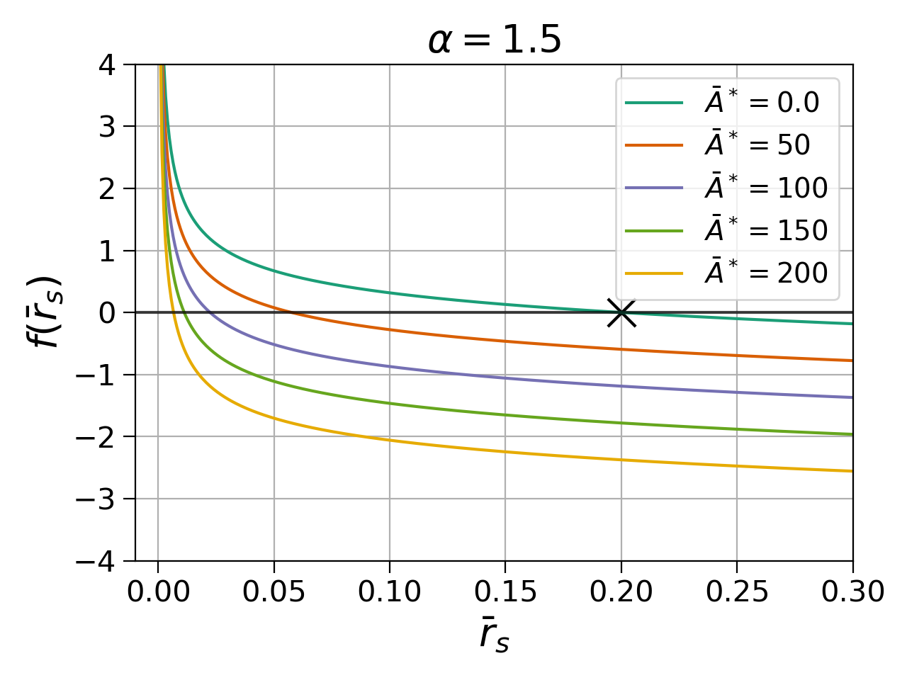
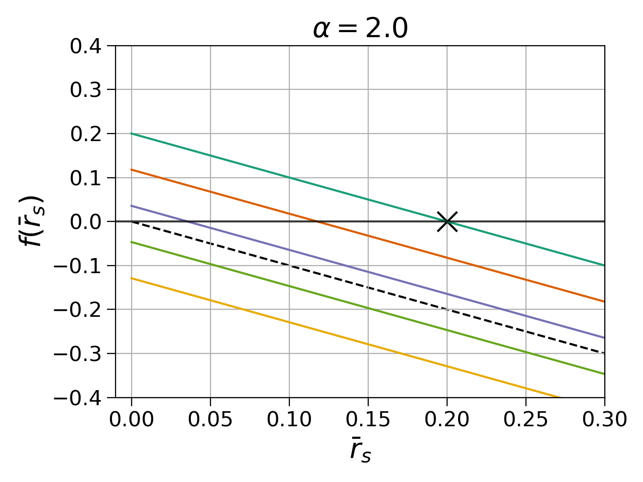
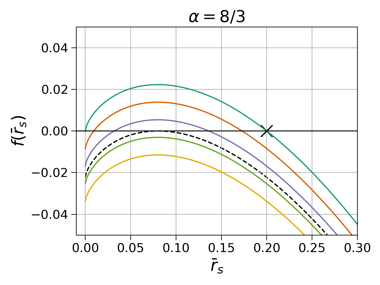
Figure 1: Solutions for $\bar{r}_{s}$ for three examples for cases 1, 2 and 3. In each panel we plot $f(\bar{r}_{s})$, as defined in Eq. (59), for $\gamma=1.4$, and for different values of the nondimensional heating rate parameter $\bar{A}^{*}$ (the labeling is the same in all three panels). Solutions for $\bar{r}_{s}$ correspond to zero-crossings of the functions $f(\bar{r}_{s})$. In case 1, with $1<\alpha<2$, we find one solution for $\bar{r}_{s}$ (see the left panel for $\alpha=1.5$). In case 2, with $\alpha=2$ (middle panel), we find one solution but only up to a maximum heating rate $\bar{A}^{*}_{\rm crit}=121.6$ (marked by the dashed black line), beyond which the solution $\bar{r}_{s}$ becomes negative. Finally, in case 3, for $\alpha>2$, the number of solutions again depends on $\bar{A}^{*}$. For the example of $\alpha=8/3$ (shown in the right panel) we find two solutions for $\bar{r}_{s}$ up to a maximum value $\bar{A}^{*}_{\rm crit}=131.8$ (marked by the dashed black line), and none beyond that value. In all three panels the cross marks the sonic radius $\bar{r}_{s}=0.2$ in the adiabatic limit (see Eq. 38). In all three cases the (outer) sonic radius decreases as the heating rate increases. In case 3 an additional inner sonic radius appears for $\bar{A}^{*}>0$ and increases for increasing heating rate, until both sonic points merge and disappear for the critical value $\bar{A}^{*}=\bar{A}^{*}_{\rm crit}$.

As a first step we will discuss solutions for the sonic radius for different parameter choices. We note that smooth and steady-state heated transonic Bondi solutions do not exist for $\gamma=5/3$, at least in our Newtonian treatment of the problem. This can be seen from Eq. (57), where the first term vanishes for $\gamma=5/3$, leaving us with

$$\bar{r}_{s}^{\alpha-1}=-\beta\bar{A}^{*}\bar{r}_{\rm ann}^{\alpha}.$$ (61)

As we discussed above, $\beta>0$ for $\alpha>1$, so that this equation will not allow real and positive solutions. We therefore conclude that heated transonic solutions are possible only for $\gamma<5/3$, which we will consider in the following. We also find that the behavior depends on the values of $\alpha$, and we therefore distinguish between three different cases, which are illustrated in Fig. 1.

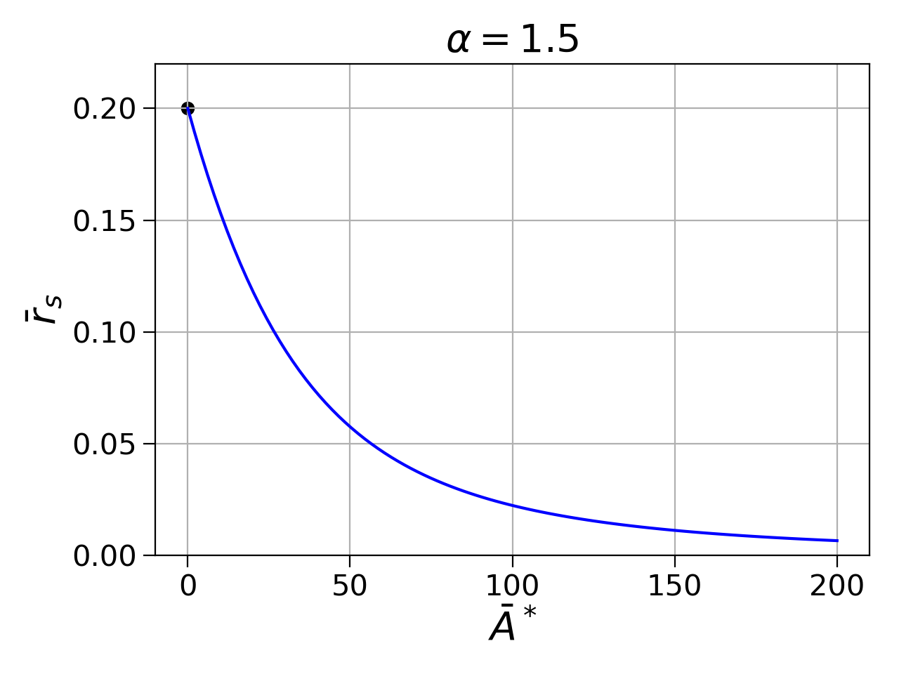
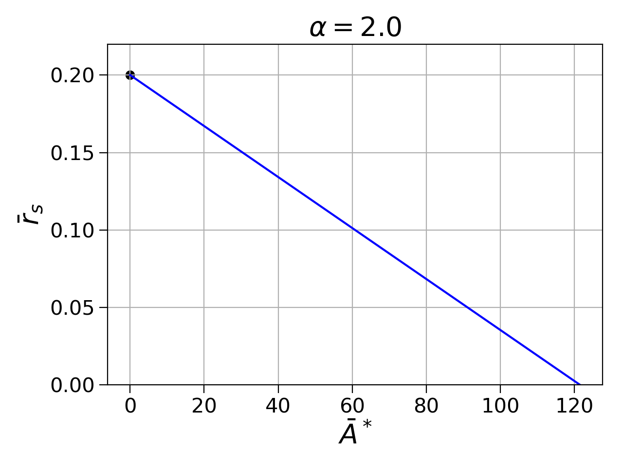
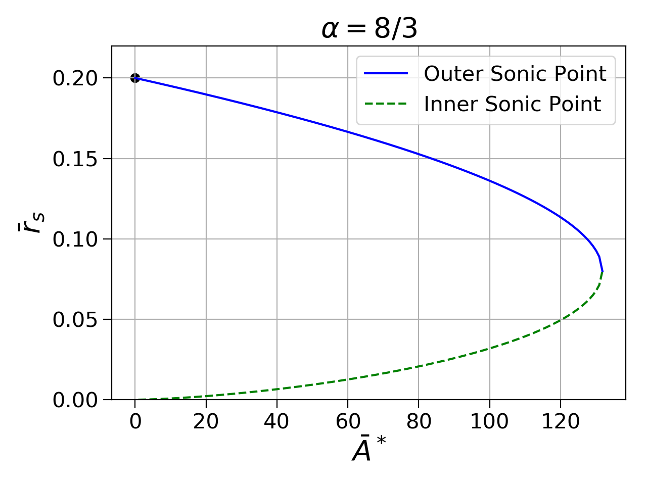
Figure 2: Values of $\bar{r}_{s}$ as a function of $\bar{A}^{*}$ for the same three examples as shown in Fig. 1, namely for $\alpha=1.5$ (left panel), $\alpha=2$ (middle panel) and $\alpha=8/3$ (right panel), and all for $\gamma=1.4$. Note that (i) a solution for $\bar{r}_{s}$ exists for all values of $\bar{A}^{*}$ for $\alpha<2$ (case 1; left panel), (ii) the linear behavior for $\alpha=2$ (case 2; middle panel), and (iii) the existence of two solutions for $\bar{A}^{*}<\bar{A}^{*}_{\rm crit}$ for $\alpha=8/3$ (case 3; right panel).

4.2.1 Case 1: $1<\alpha<2$

In the regime $1<\alpha<2$ we find one single real value for $\bar{r}_{s}$ for suitable combinations of $\bar{A}^{*}$ and $\gamma<5/3$. An example, for $\gamma=1.4$, is shown in the left panel of Fig. 1, where the cross denotes the sonic radius $\bar{r}_{s}=0.2$ in the adiabatic limit (see Eq. 38). Note that the sonic radius decreases with increasing heating parameter $\bar{A}^{*}$, indicating that heating prevents the flow from becoming transonic until it gets closer to the black hole. We also show $\bar{r}_{s}$ as a function of $\bar{A}^{*}$ in the left panel of Fig. 2.

4.2.2 Case 2: $\alpha=2$

In the special case of $\alpha=2$, Eq. (59) reduces to the linear equation

$$\bar{r}_{s}=\frac{5-3\gamma}{4}-\beta\bar{A}^{*}\bar{r}_{\rm ann}^{2}\hfill(\alpha=2)$$ (62)

providing us with a unique value of $\bar{r}_{s}$ (see also the middle panels in Figs. 1 and 2). Evidently, we can find positive solutions for $\bar{r}_{s}$ only for

$$\bar{A}^{*}<\bar{A}^{*}_{\rm crit}=\frac{5-3\gamma}{4}\frac{1}{\beta\bar{r}_{\rm ann}^{2}}.\hfill(\alpha=2)$$ (63)

In particular, we find $\bar{A}^{*}_{\rm crit}=0$ for $\gamma=5/3$, consistent with our discussion above. As in case 1, increasing the heating rate will decrease the sonic radius.

4.2.3 Case 3: $\alpha>2$

An example for the case $\alpha>2$, for $\alpha=8/3$, is shown in the right panel of Fig. 1. The cross again marks the sonic radius $\bar{r}_{s}=0.2$ in the adiabatic limit with $\bar{A}^{*}=0$. For $\bar{A}^{*}>0$ an inner sonic point emerges, suggesting that, as the gas accretes, it becomes supersonic at the outer sonic point, but does not remain supersonic.

To find the critical value $\bar{A}^{*}_{\rm crit}$ above which no transonic radius exists we consider Eq. (59) an equation for $\bar{A}^{*}$ as a function of $\bar{r}_{s}$ rather than the other way around (effectively flipping the axes in the right panel of Fig. 2). The critical value $\bar{A}^{*}_{\rm crit}$ is then given by the point at which the derivative $d\bar{A}^{*}/d\bar{r}_{s}$ vanishes, which yields

$$\bar{r}_{s}^{\rm crit}=\frac{\alpha-2}{\alpha-1}\frac{5-3\gamma}{4}.\hfill(\alpha>2)$$ (64)

Inserting this into (59) and solving for $\bar{A}^{*}_{\rm crit}$ yields

$$\bar{A}^{*}_{\rm crit}=\frac{1}{\alpha-1}\frac{(\bar{r}_{s}^{\rm crit})^{\alpha-1}}{\beta}\frac{1}{\bar{r}_{\rm ann}^{\alpha}}.\hfill(\alpha>2)$$ (65)

We again find that $\bar{A}^{*}_{\rm crit}=0$ for $\gamma=5/3$, consistent with our discussion above. For other suitable values of $\gamma<5/3$ and $\bar{A}^{*}<\bar{A}^{*}_{\rm crit}$, however, we find two solutions for the sonic radius $\bar{r}_{s}$.

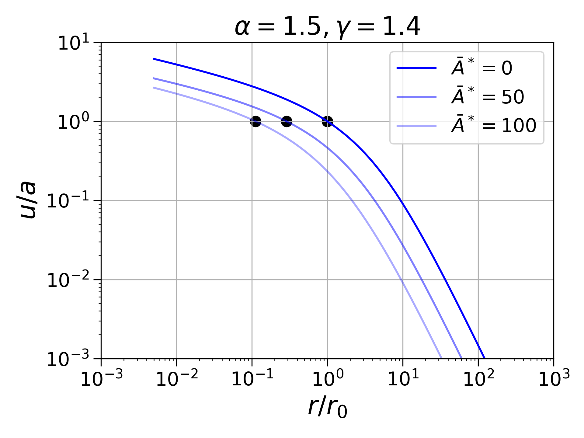
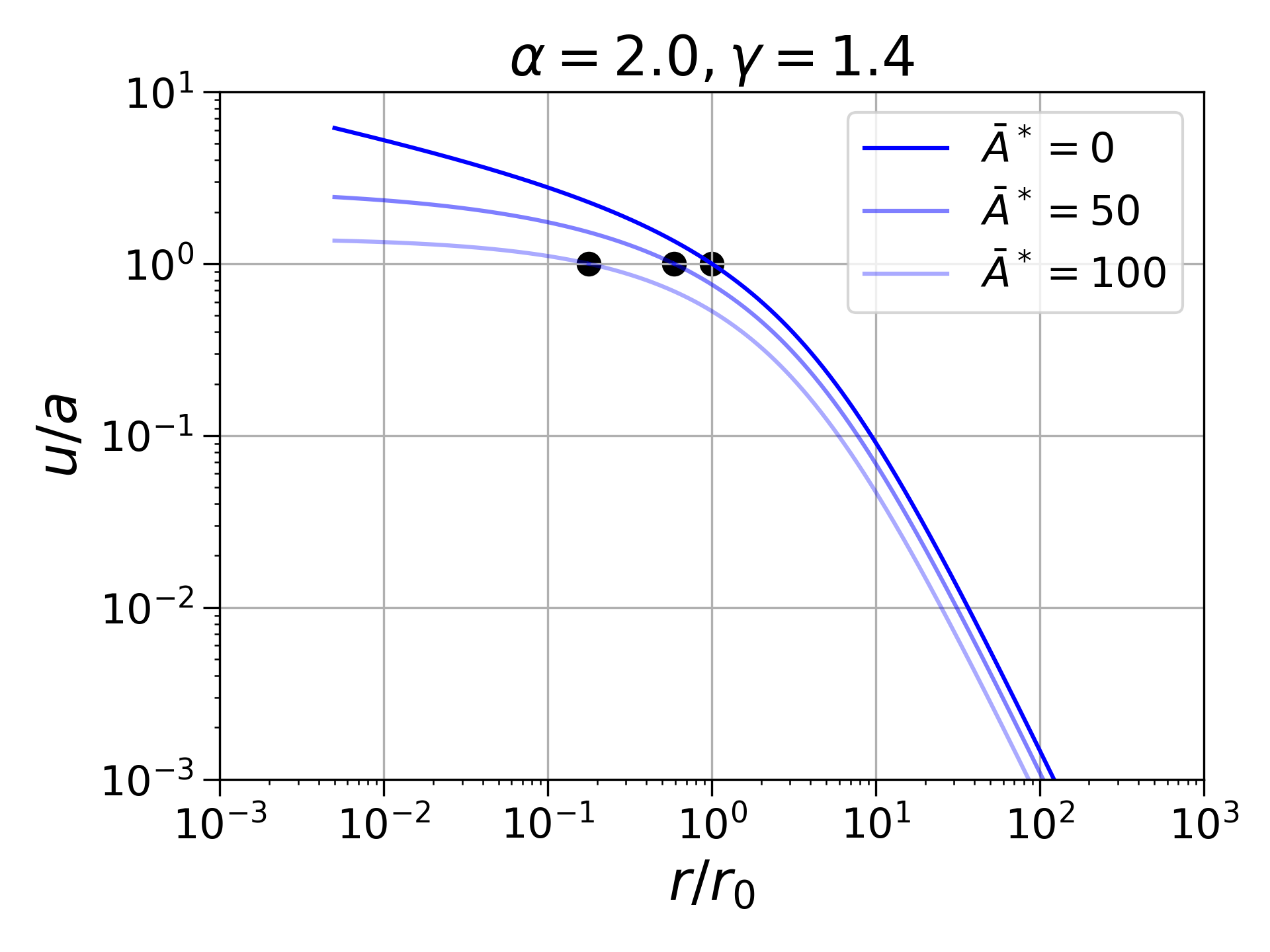
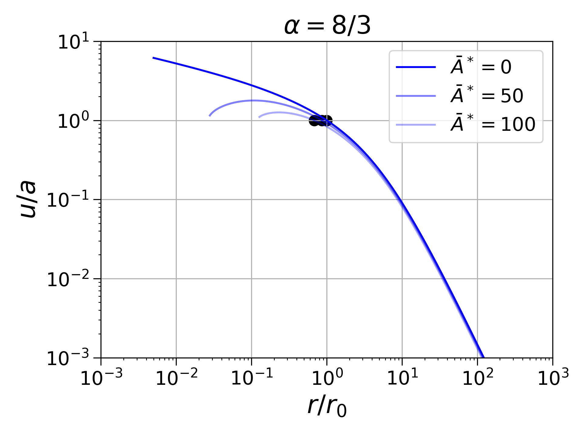
Figure 3: Examples of fluid profiles with $\gamma=1.4$ for the same three examples as shown in Figs. 1 and 2. The left panel shows the fluid velocity $u$ for $\alpha=1.5$, the middle panel for $\alpha=2.0$, and the right panel for $\alpha=8/3$. The (outer) sonic points, at which $u=a$, are marked by dots. For $\alpha=2.0$, the sonic radius $\bar{r}_{s}$ goes to zero as $\bar{A}^{*}$ approaches $\bar{A}^{*}_{\rm crit}$. For $\alpha=8/3$, the fluid approaches a singular inner sonic point.

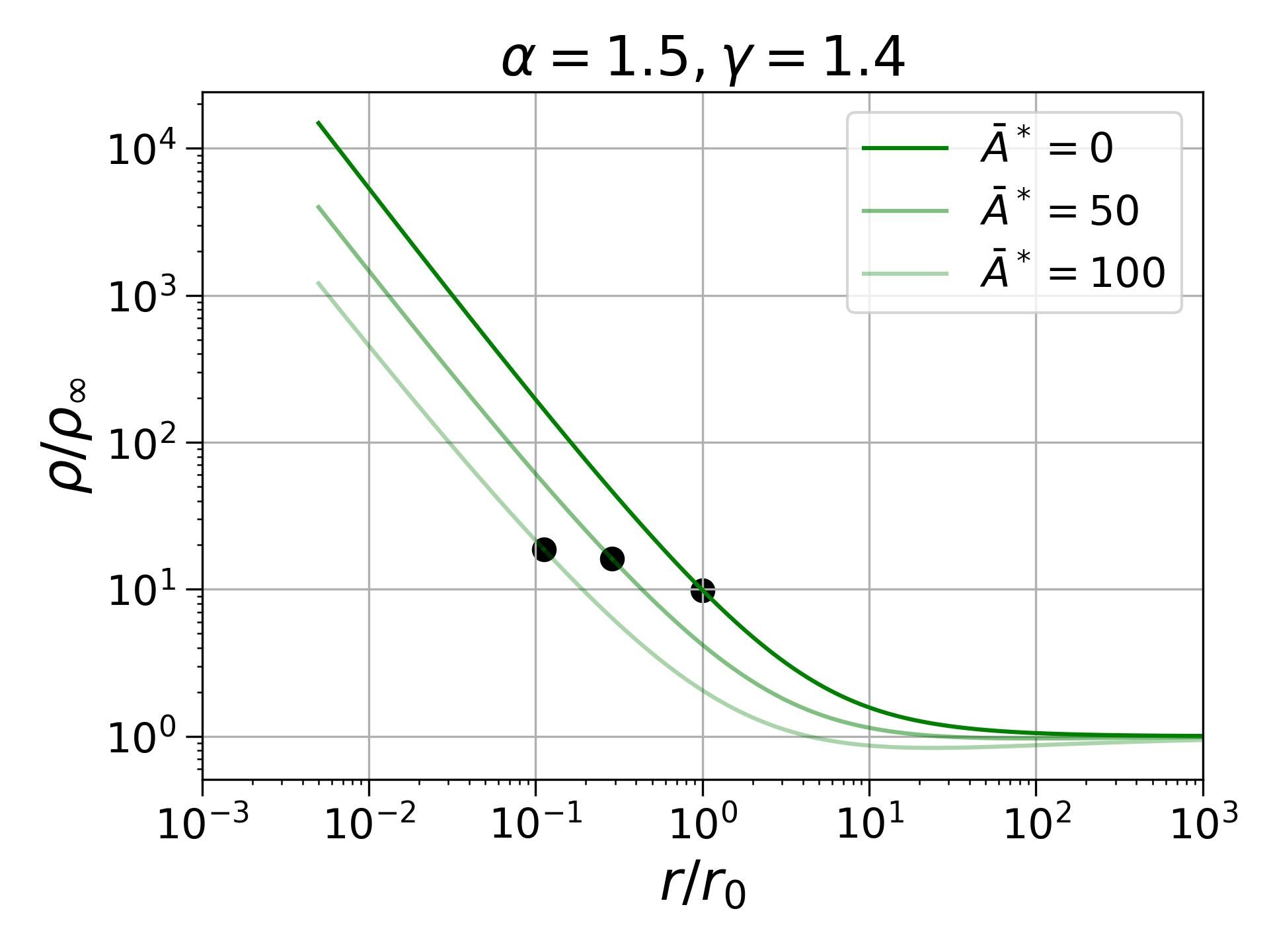
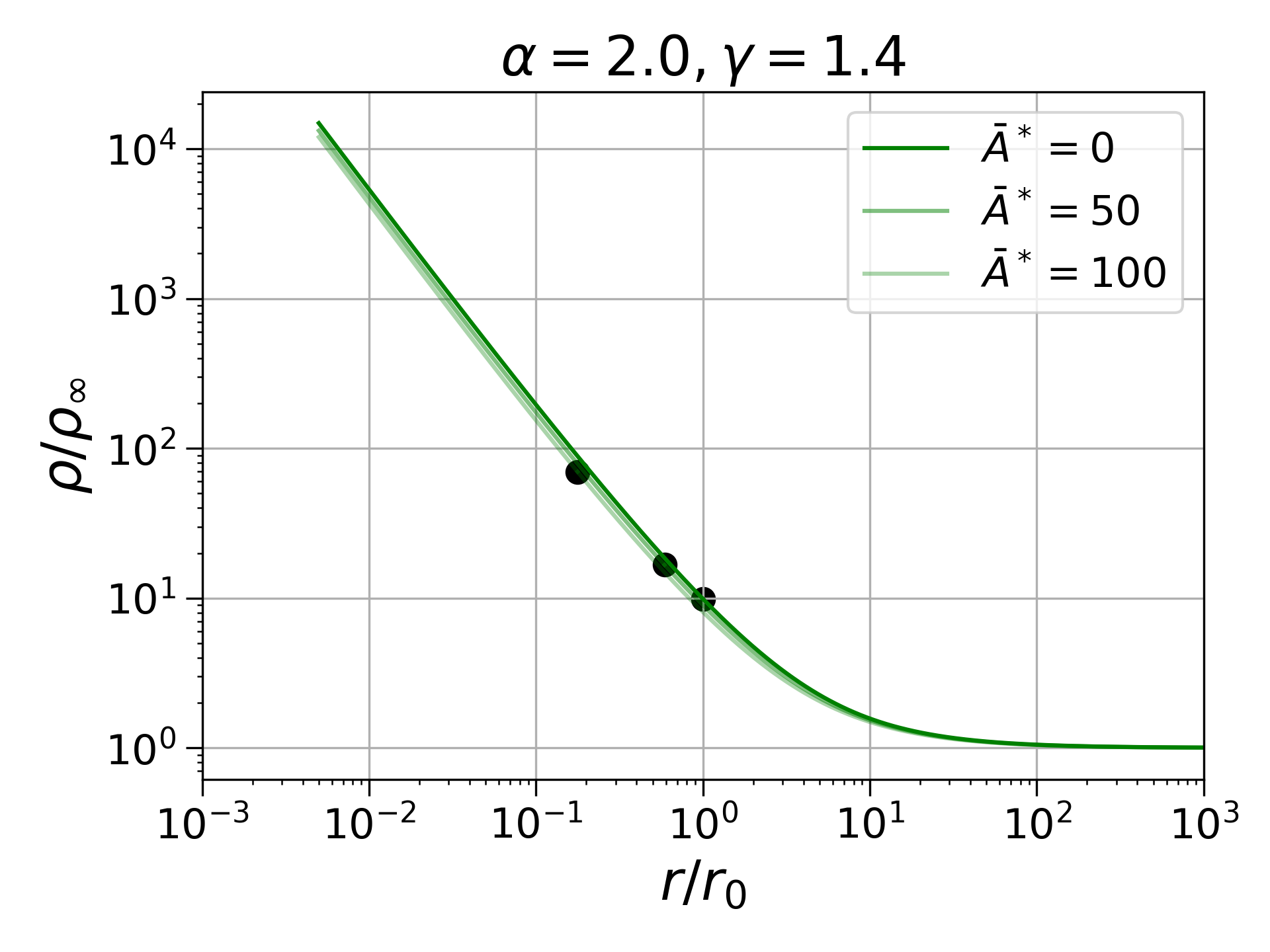
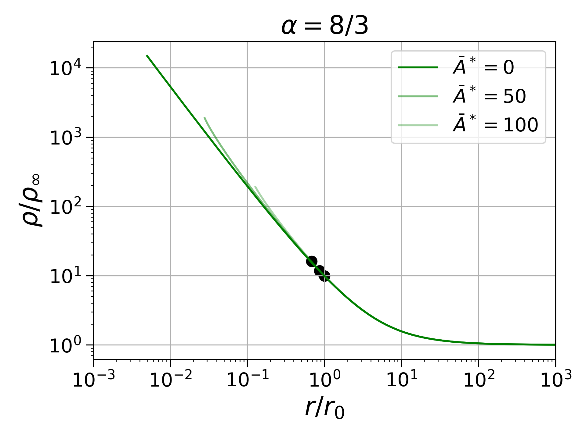
Figure 4: Same as Fig. 3, but for density profiles.

As described in Section 4.1, constructing fluid flow profiles requires an expansion about the sonic radii $\bar{r}_{s}$, since the differential equations (48) and (49) cannot be evaluated directly at those points. Applying l’Hôpital’s rule results in a quadratic equation for $\bar{u}^{\prime}$. In all cases that we have considered, this equation had real solutions at the outer sonic point, allowing for smooth flow there, but only imaginary solutions at the inner sonic point. This is an indication that it is impossible to construct smooth solutions across the inner sonic point, where the fluid’s speed drops from being supersonic to subsonic. Instead, we might expect that shocks, and hence discontinuities in the fluid’s flow, develop at this point (see also Chang & Ostriker, 1985; Park & Ostriker, 1998). As a result, we conclude that in the regime considered, for $\alpha>2$, no smooth, steady-state transonic solutions describing spherical accretion exist.

For $\alpha\geq 3$ we might find even more solutions for $\bar{r}_{s}$, but we do not pursue this possibility in greater detail, since this range of parameters appears less relevant astrophysically.

4.3 Finding fluid profiles and the accretion rate

As outlined in Section 4.1, finding the accretion rate involves an iterative “shooting method" to match to the boundary conditions at $\bar{r}\rightarrow\infty$. This involves integrating the differential equations (48), (49) and (54), which, in turn, involves applying l’Hôpital’s rule at the (outer) sonic radius $\bar{r}_{s}$. Once $\bar{K}_{s}$ has been found, the equations can be integrated both outwards and inwards in order to find the profiles of the fluid flow. We show examples for the three different cases with $\alpha<2$, $\alpha=2$ and $\alpha>2$ in Figs. 3 and 4.

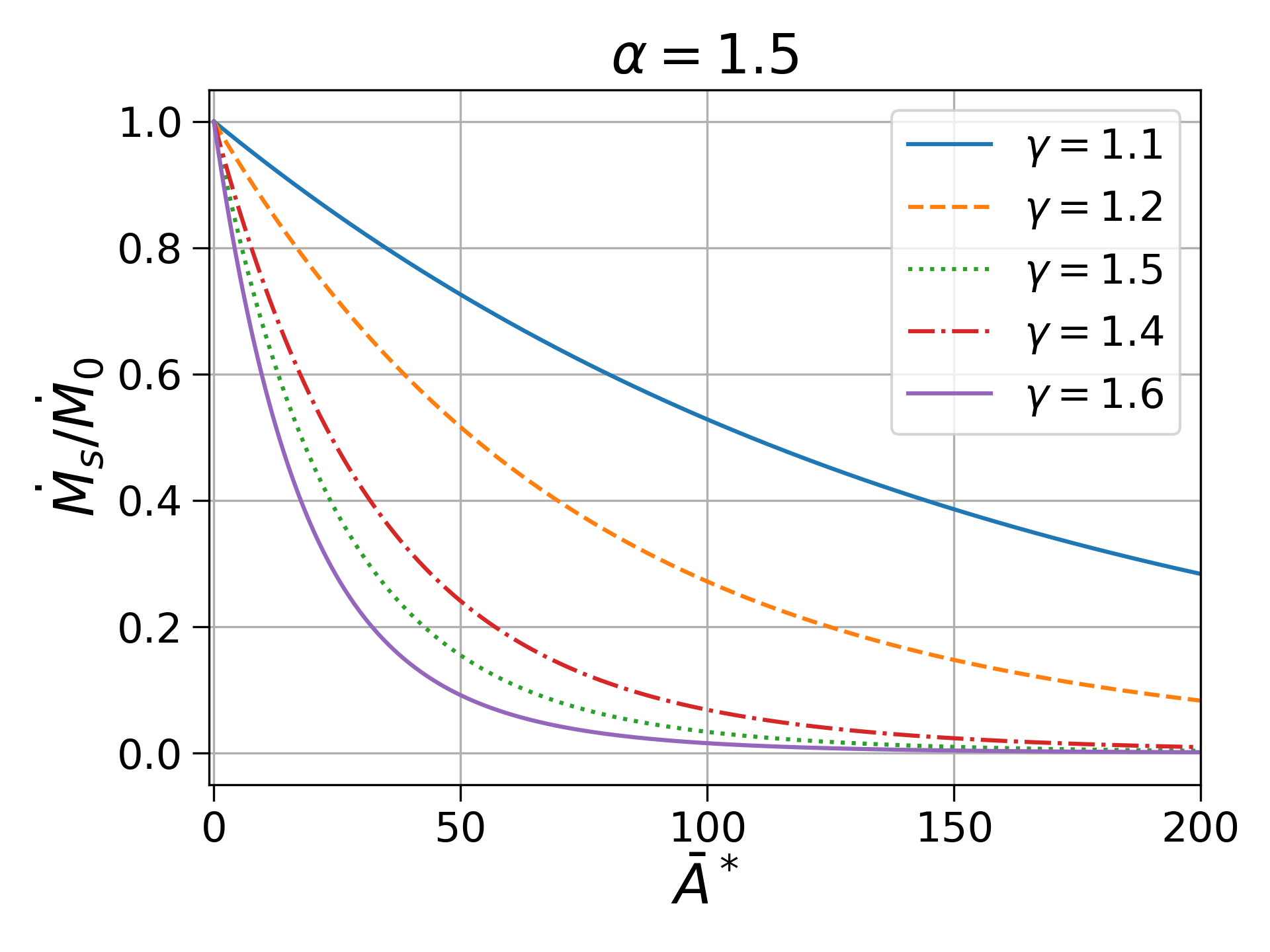
Figure 5: The accretion rate $\dot{M}_{s}/\dot{M}_{0}$ for transonic flow as a function of $\bar{A}^{*}$ for different sets of parameters. The upper panel shows results for fixed $\gamma=1.4$ and varying values of $1<\alpha<2$ while the lower panel shows results for a fixed $\alpha=1.5$ and varying values of $1<\gamma<5/3$. As expected, the accretion rate decreases with increasing heating parameter $\bar{A}^{*}$. We find that the accretion rate decreases more rapidly as the DM power law heating $\alpha$ approaches $1$ and the adiabatic index $\gamma$ approaches $5/3$.

As we discussed above, $\alpha>2$ leads to the existence of a second inner sonic point, across which we cannot find smooth solutions (see also the right panel in Fig. 3). We therefore focus on $\alpha<2$ here. We show examples for different values of $1<\alpha<2$ and $\gamma=1.4$, which we have previously considered in the left panels of Figs. 1 through 4, and show a graph of $\dot{M}/\dot{M}_{0}$ as a function of $\bar{A}^{*}$ in the upper panel of Fig. 5. We also show a graph for $\dot{M}/\dot{M}_{0}$ as a function of $\bar{A}^{*}$ for different values of $1<\gamma<5/3$ and $\alpha=1.5$ in the lower panel of Fig. 5. As anticipated, the heating due to DM annihilation reduces the accretion rate.

5 Heated subsonic flow

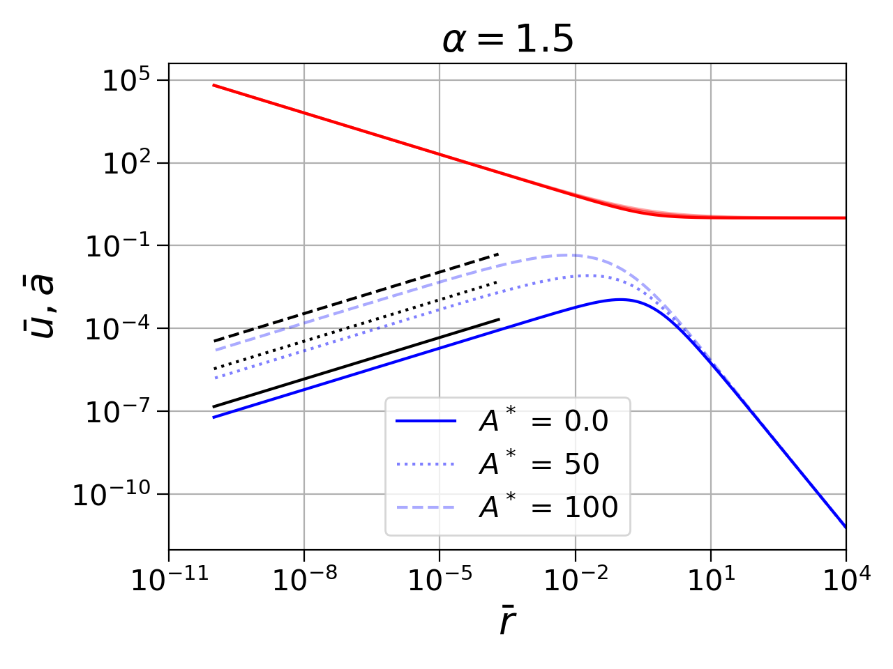
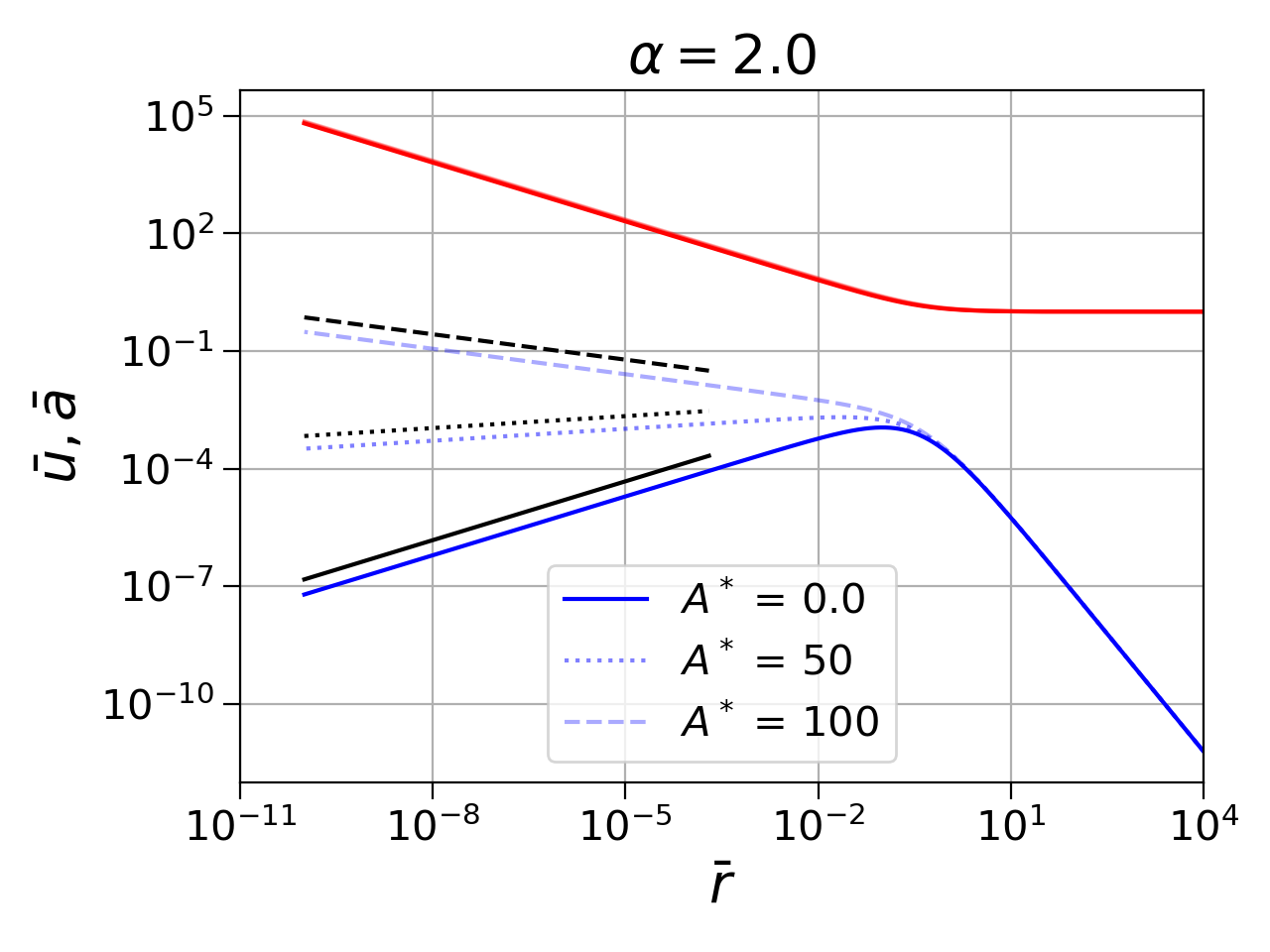
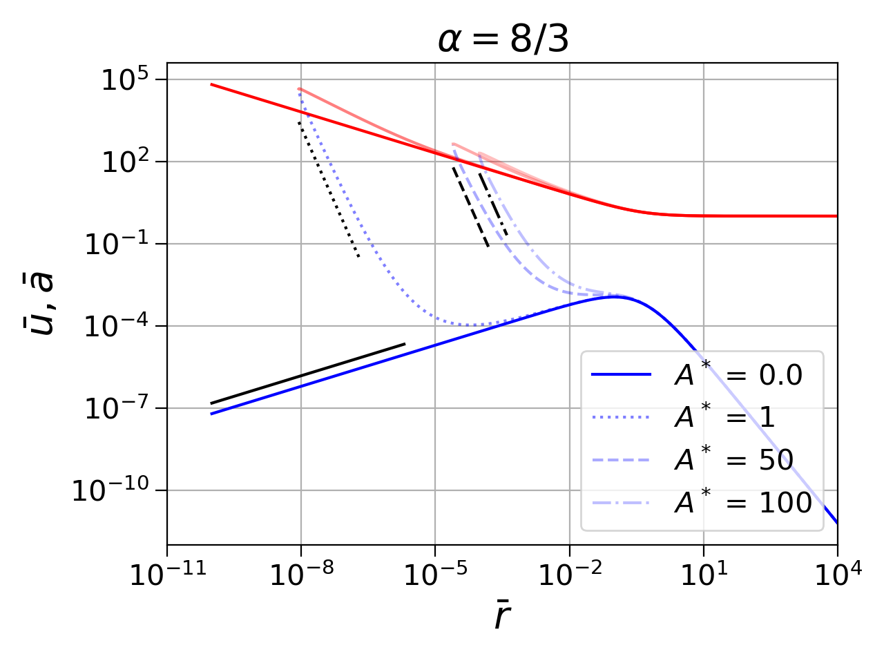
Figure 6: Subsonic flow profiles for $\gamma=1.4$, with $\alpha=1.5$ in the left panel, $\alpha=2$ in the middle panel, and $\alpha=8/3$ in the right panel. We show results for selected values of $\bar{A}^{*}$ in all three cases, with the lower (blue) lines showing the fluid velocity $u$, and the upper (red) lines showing the sound speed $a$. Also included are the expected power laws for the fluid velocity $u$, as given by Eqs. (71), (78) and (86). In case 1 (left panel, Section 5.1) the scaling of the fluid profiles approach the same power laws as their adiabatic counterparts, in case 2 (middle panel, Section 5.2) the power law exponent depends on the heating rate, and in case 3 (left panel, Section 5.3) heating results in the appearance of a singular sonic point at small radii.

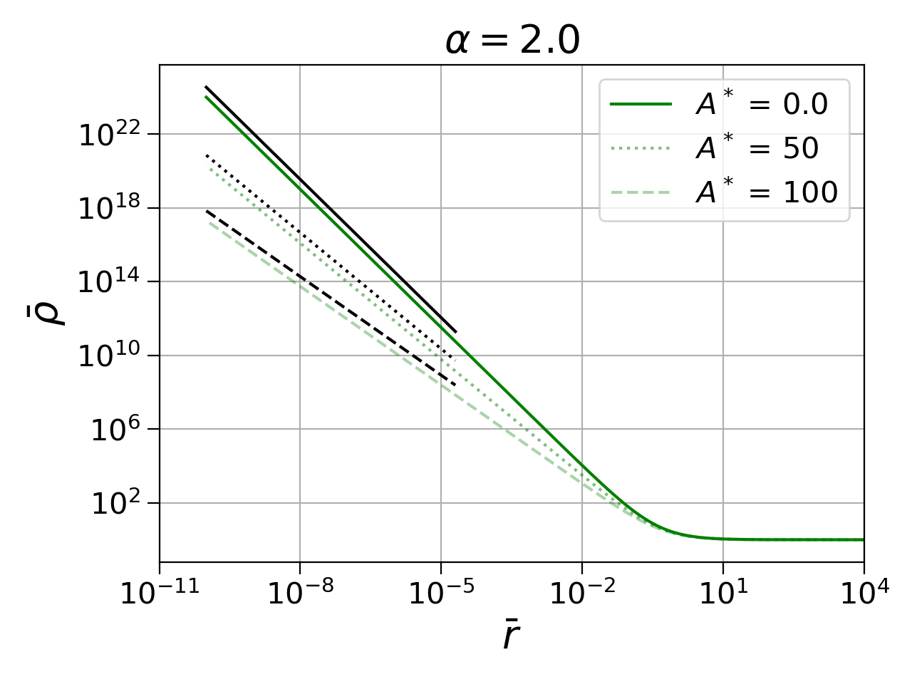
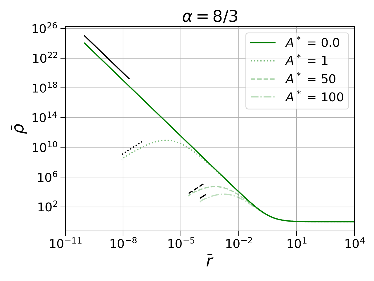
Figure 7: Same as Fig. 6, but for density profiles.

While we believe that, when it exists, supersonic accretion onto black holes is the most likely astrophysically (see, e.g., Appendix G in Shapiro & Teukolsky (1983), which shows that subsonic flow as gas approaches a black hole is ruled out in a general relativistic treatment of the adiabatic problem and that the flow will be driven supersonic), we also consider effects of heating on subsonic flows in this Section. As before, we will treat the cases $\alpha<2$, $\alpha=2$, and $\alpha>2$ separately.

To construct subsonic solutions, we pick an accretion rate less than the corresponding transonic accretion rate, $\dot{\bar{M}}<\dot{\bar{M}}_{s}$. We also pick a large radius $\bar{r}_{\rm init}\gg\bar{r}_{0}$ and assume $\bar{K}\simeq 1$ there. We express $\bar{u}$ in terms of (56), $\bar{a}$ in terms of (46) and insert these into the Bernoulli equation (57), yielding an equation for $\bar{\rho}$ at $\bar{r}_{\rm init}$. With these initial values, we then integrate (48), (49) and (54) inwards from $\bar{r}_{\rm init}$.

5.1 Case 1: $\alpha<2$

We show an example for subsonic flow with $\alpha<2$ in the left panel of Fig. 6. In this case, the fluid profiles appear to approach the same power-law behavior for $\bar{r}\rightarrow 0$ as in the adiabatic case. This behavior can be understood from the following arguments. Starting with the Bernoulli equation (57), we assume subsonic flow with $\bar{u}\ll\bar{a}$ as well as $\bar{a}\gg 1$ (i.e. $a\gg a_{\infty}$). The equation will be dominated by the gravitational term at small $\bar{r}$ when $\alpha<2$, and the heating term can be neglected. We therefore have

$$\bar{a}^{2}\simeq\frac{\gamma-1}{\bar{r}},\hfill(\bar{r}\rightarrow 0,~{}\alpha<2)$$ (66)

just like in the adiabatic case (see Eq. (14.3.28) in ST). Inserting this into (46) we obtain

$$\bar{\rho}=\left(\frac{\bar{a}^{2}}{\bar{K}}\right)^{1/(\gamma-1)}\simeq\left(\frac{\gamma-1}{\bar{K}\bar{r}}\right)^{1/(\gamma-1)},\hfill(\bar{r}\rightarrow 0,~{}\alpha<2)$$ (67)

(compare Eq. (14.3.29) in ST). In order to find an asymptotic scaling for $\bar{K}$ we now insert (67) into (54) to find

$$\bar{K}^{\prime}\simeq-\gamma\frac{\bar{A}^{*}\bar{r}_{\rm ann}^{\alpha}\bar{K}}{\bar{r}^{\alpha-1}}.\hfill(\bar{r}\rightarrow 0,~{}\alpha<2)$$ (68)

Integration yields

$$\bar{K}\propto\exp\left(-\gamma\bar{A}^{*}\bar{r}_{\rm ann}^{\alpha}\bar{r}^{2-\alpha}/(2-\alpha)\right),\hfill(\bar{r}\rightarrow 0,~{}\alpha<2)$$ (69)

so that $\bar{K}$ approaches a (finite) constant as $\bar{r}\rightarrow 0$. Inserting this result back into (67) we now have

$$\bar{\rho}\propto\bar{r}^{-1/(\gamma-1)},\hfill(\bar{r}\rightarrow 0,~{}\alpha<2)$$ (70)

and, using the accretion rate (56),

$$\bar{u}\propto\bar{r}^{-(2\gamma-3)/(\gamma-1)},~{}~{}~{}~{}\hfill~{}~{}(\bar{r}\rightarrow 0,~{}\alpha<2)$$ (71)

(see Eq. (14.3.30) in ST). For $\alpha<2$ we therefore expect the exact same power-law behavior for $\bar{r}\rightarrow 0$ as in the adiabatic case. For $\gamma=5/3$, in particular, we recover the free-fall behavior $\bar{u}\propto\bar{r}^{-1/2}$ and $\bar{\rho}\propto\bar{r}^{-3/2}$. Even in this case, $\bar{u}$ and $\bar{a}$ increase with the same power law, meaning that a solution with $\bar{u}<\bar{a}$ will remain subsonic. We show examples of this behavior in the left panels in Figs. 6 and 7, where the expected power laws are marked by the black lines.

5.2 Case 2: $\alpha=2$

We find very different asymptotic behavior in the special case $\alpha=2$. In this case, the heating term scales with the same power as the gravitational term in the Bernoulli equation (57), so that, considering the same limit as before, we now obtain

$$\bar{a}^{2}\simeq(\gamma-1)\frac{1+\bar{A}^{*}\bar{r}_{\rm ann}^{2}}{\bar{r}}\hfill(\bar{r}\rightarrow 0,~{}\alpha=2)$$ (72)

instead of (66). From (46) we now have

$$\bar{\rho}\approx\left((\gamma-1)\frac{1+\bar{A}^{*}\bar{r}_{\rm ann}^{2}}{\bar{K}\bar{r}}\right)^{1/(\gamma-1)},\hfill(\bar{r}\rightarrow 0,~{}\alpha=2)$$ (73)

which we insert into (54)

$$\bar{K}^{\prime}\simeq-\gamma\frac{\bar{A}^{*}\bar{r}_{\rm ann}^{2}}{1+\bar{A}^{*}\bar{r}_{\rm ann}^{2}}\frac{\bar{K}}{\bar{r}}.\hfill(\bar{r}\rightarrow 0,~{}\alpha=2)$$ (74)

Integration now yields

$$\bar{K}\propto\bar{r}^{-\gamma\delta},\hfill(\bar{r}\rightarrow 0,~{}\alpha=2)$$ (75)

where we have abbreviated

$$\delta\equiv\frac{\bar{A}^{*}\bar{r}_{\rm ann}^{2}}{1+\bar{A}^{*}\bar{r}_{\rm ann}^{2}}.$$ (76)

Inserting (75) into (73) now yields

$$\bar{\rho}\propto\bar{r}^{-(1-\gamma\delta)/(\gamma-1)},\hfill(\bar{r}\rightarrow 0,~{}\alpha=2)$$ (77)

and, using (56) again,

$$\bar{u}\propto\bar{r}^{-(2\gamma-3+\gamma\delta)/(\gamma-1)}.\hfill(\bar{r}\rightarrow 0,~{}\alpha=2)$$ (78)

Interestingly, the power-law scaling now depends on the heating rate $\bar{A}^{*}$ through $\delta$. We show examples for this behavior in the middle panels of Figs. 6 and 7, where we again find excellent agreement between our numerical result and the power-law behavior expected from the above arguments. Note that we have $\delta\rightarrow 0$ in the adiabatic limit, in which case our results above reduce to those of Case 1 in Section 5.1, as expected. For sufficiently small heating rate, and hence sufficiently small $\delta$, the fluid velocity $\bar{u}$ still grows more slowly than the sound speed $\bar{a}$ as $\bar{r}\rightarrow 0$, so that a subsonic solution will remain subsonic. For

$$\delta>\delta_{\rm crit}=\frac{5-3\gamma}{2\gamma},$$ (79)

corresponding to a heating rate

$$\bar{A}^{*}>\bar{A}^{*}_{\rm crit}=\frac{5-3\gamma}{5(\gamma-1)}\,\bar{r}_{\rm ann}^{-2},$$ (80)

however, $\bar{u}$ increases more rapidly than $\bar{a}$ as $\bar{r}\rightarrow 0$, suggesting that this solution will not remain subsonic for arbitrarily small $\bar{r}$. This contradicts our assumption $\bar{u}\ll\bar{a}$, of course, so that our approximations will no longer remain accurate. We also caution that, for DM heating, the exponent $\alpha$ would probably drop to a smaller value at $\bar{r}\sim\bar{r}_{\rm ann}$ (see Section 2), which we ignored in our treatment here. The appearance of a critical heating rate is reminiscent of that for transonic flow with $\alpha=2$ in Section 4.2.2.

5.3 Case 3: $\alpha>2$

Finally we consider the case $\alpha>2$. Making the same assumptions of $\bar{u}\ll\bar{a}$ and $\bar{a}\gg 1$ as before in the Bernoulli equation (57), we now see that the heating term dominates at small $\bar{r}$, so that we may approximate

$$\frac{\bar{a}^{2}}{\gamma-1}\approx\frac{\bar{A}^{*}}{\alpha-1}\frac{\bar{r}_{\rm ann}^{\alpha}}{\bar{r}^{\alpha-1}}\hfill(\bar{r}\rightarrow 0,~{}\alpha>2)$$ (81)

(instead of (66) and (72)). From (46) we then have

$$\bar{\rho}\approx\left(\frac{\gamma-1}{\alpha-1}\frac{\bar{A}^{*}}{\bar{K}}\frac{\bar{r}_{\rm ann}^{\alpha}}{\bar{r}^{\alpha-1}}\right)^{1/(\gamma-1)}.\hfill(\bar{r}\rightarrow 0,~{}\alpha>2)$$ (82)

Inserting (82) into (54) yields

$$\bar{K}^{\prime}\approx-\gamma(\alpha-1)\frac{\bar{K}}{\bar{r}},\hfill(\bar{r}\rightarrow 0,~{}\alpha>2)$$ (83)

which we can integrate to obtain

$$\bar{K}\propto\bar{r}^{-\gamma(\alpha-1)}.\hfill(\bar{r}\rightarrow 0,~{}\alpha>2)$$ (84)

As before, we now insert (84) back into (82) to find

$$\bar{\rho}\propto\bar{r}^{\alpha-1},\hfill(\bar{r}\rightarrow 0,~{}\alpha>2)$$ (85)

and combine this with the accretion rate (56) to find

$$\bar{u}\propto\bar{r}^{-(\alpha+1)}.\hfill(\bar{r}\rightarrow 0,~{}\alpha>2)$$ (86)

Note that the power law exponents for the fluid variables $\bar{a}$, $\bar{\rho}$ and $\bar{u}$ are independent of both $\gamma$ and the heating rate in this case, and instead depend on $\alpha$ only. Also note that, for all $\alpha>2$, $\bar{u}$ increases more rapidly than

$$\bar{a}\propto\bar{r}^{-(\alpha-1)/2}\hfill(\bar{r}\rightarrow 0,~{}\alpha>2)$$ (87)

with decreasing $\bar{r}$. While our estimates assume that $\bar{u}\ll\bar{a}$, they again suggest that this assumption will break down at some sufficiently small $\bar{r}$, once the heating term dominates. In fact, these results suggest that “subsonic" solutions may not remain subsonic to arbitrarily small radii, instead they may encounter a sonic point at some some radius $\bar{r}$, where $\bar{u}=\bar{a}$. This is exactly what our numerical explorations of this regime suggest. We show examples in the right panels of Figs. 6 and 7, where we have also included the expected power-law behavior. As one might expect, for larger values of $\bar{A}^{*}$ the flow will deviate from the adiabatic flow, and be dominated by the heating term, starting at larger values of $\bar{r}$. For small heating we find very good agreement between the numerical results and the expected power law, while for larger heating the assumption $\bar{u}\ll\bar{a}$ appears to be violated before $\bar{u}$ can approach the heating-dominated power law.

For generic accretion rate, the sonic point found in this process will not satisfy the conditions laid out in Section 4.1; in particular the numerators and denominators on the right-hand sides of Eqs. (48) and (49) will not have simultaneous roots, so that these solutions will not describe smooth fluid flow.

Combining this finding with that of Section 4.2.3 we conclude that, for $\alpha>2$, we can find neither supersonic nor subsonic solutions that describe smooth, steady-state spherical accretion for all radii. We will comment on this result, as well as its limitations, in more detail in Section 7. In particular, we remind the reader that we have assumed a constant $\gamma_{\rm sp}$ for all $r$ in the DM density distribution (2), whereas we would expect $\gamma_{\rm sp}$ to switch to $\gamma_{\rm ann}$ at $r_{\rm ann}\sim r_{\rm a}/20$. Clearly, relaxing this assumption will affect the findings for very small $r$ in this section.

6 Applications to Sgr A^∗

Figure 8: The accretion rate $\dot{M}/\dot{M}_{0}$ as a function of the heating parameter $\bar{A}^{*}$, for $\alpha=1.5$ and $\gamma=1.4$. The solid (purple) line represents numerical results for transonic solutions (see Section 4), while the straight lines represent the hyperbolae (90) for efficiencies $\epsilon=$ 0.01, 0.001, 0.003327, and 0.0001. Intersections of the solid line with the hyperbolae represent viable solutions for the DM parameters assumed in (89), and identify the associated accretion rates $\dot{M}/\dot{M}_{0}$. The solutions identified by the solid square and the cross, for example, represent spherically symmetric, steady-state accretion for which the heating by DM annihilation has reduced the accretion rate by a factor of about $0.37$ and about $1\times 10^{-3}$ respectively. For the solution marked by the open square, which corresponds to the same heating efficiency as that marked by the cross, the accretion rate is reduced by a factor of $0.988$ only (see text for a discussion). We show flow profiles for the solutions represented by the cross and the two squares in Fig. 9.

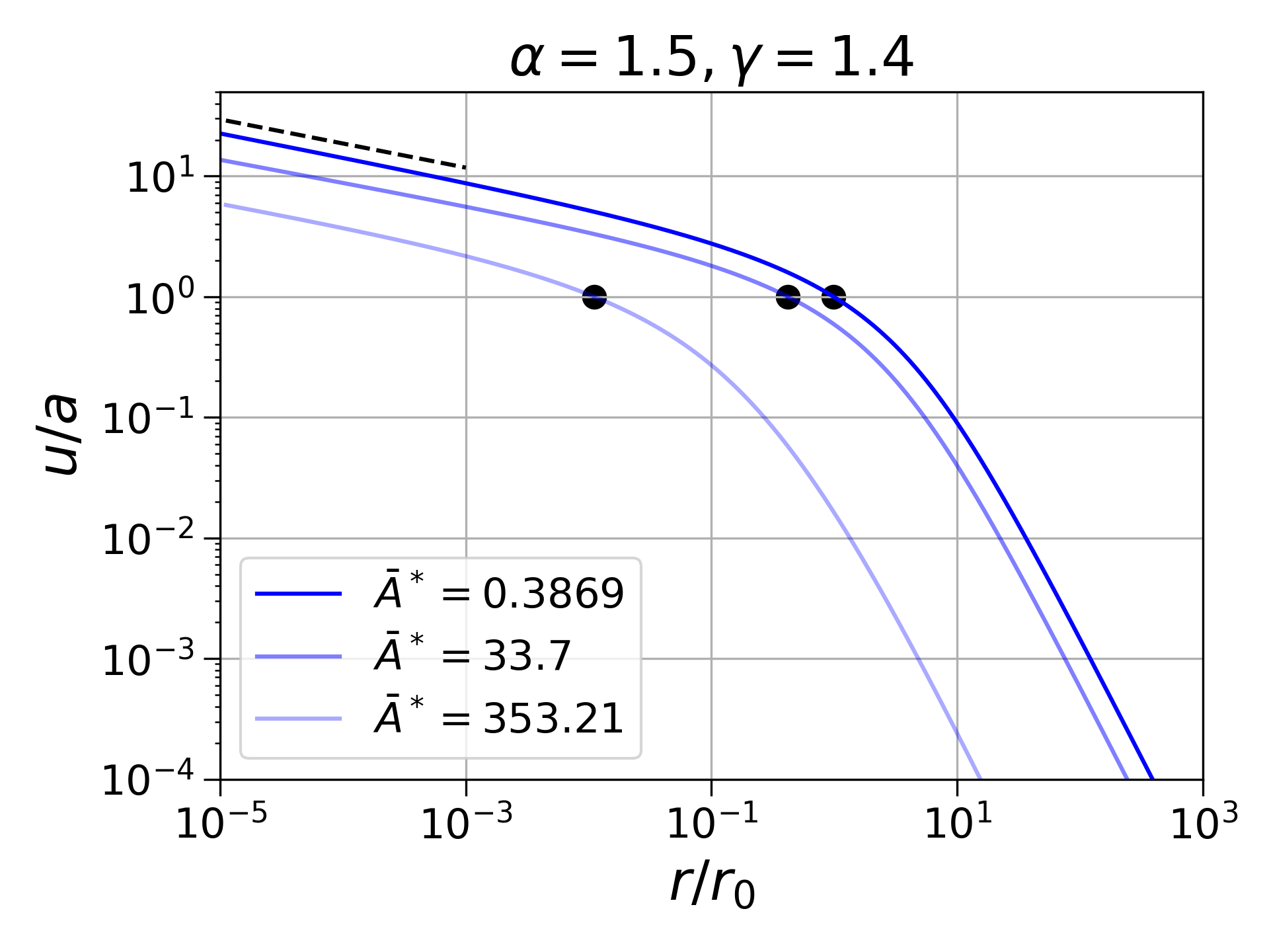
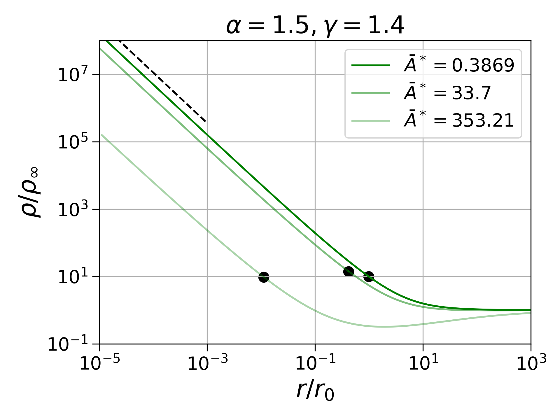
Figure 9: Fluid flow profiles for the heated, transonic accretion solutions for $\gamma=1.4$ and $\alpha=1.5$ and marked by the cross, and the solid and open squares in Fig. 8. For the solution denoted by the cross in Fig. 8 the accretion rate is reduced by a factor of about $1\times 10^{-3}$ below the adiabatic Bondi accretion rate. For this solution, displayed as the lightest solid line, $\bar{A}*=353.21$. For the solution denoted by the solid (open) square in Fig. 8, for which $\bar{A}^{*}=33.7$ ($\bar{A}^{*}=0.3869$), the accretion rate is reduced by a factor of about $0.37$ ($0.988$) below the corresponding adiabatic Bondi accretion rate. For Sgr A^∗, $\rho_{\infty}\approx 3\times 10^{-23}$ g cm^-3, and $r_{s}\approx 0.06$ pc. Included in the fluid profiles are the expected power laws for the transonic fluid velocity, $u$ $\approx r^{-1/2}$, and fluid density, $\rho$ $\approx r^{-3/2}$ (see Eqs. (14.3.24) and (14.3.26) in ST).

In this Section we explore whether, for reasonable choices of DM parameters, heating by DM annihilation could explain the low accretion rates observed for Sgr A^∗ in the GC, with $\dot{M}/\dot{M}_{0}\sim 10^{-3}$. Our estimates in Section 2 suggest that DM annihilation may have an order unity effect, and we will now re-examine these effects in the context of transonic solutions for simple Bondi accretion.

In order to evaluate our results quantitatively for DM parameters considered realistic for the environment of Sgr A^∗ in the GC, we first need to express the heating parameter $\bar{A}^{*}$ in terms of the DM parameters. This is complicated by the fact that $A^{*}$, and hence the nondimensional version $\bar{A}^{*}$, depends on the accretion rate $\dot{M}$ (see eq. (34)), which, in turn, is a result of a calculation for a given value of $\bar{A}^{*}$. In order to disentangle these dependencies we use (47) and (34) to write

$$\bar{A}^{*}=\frac{r_{a}}{a_{\infty}^{2}}A^{*}=\frac{4\pi\Gamma_{0}r_{\rm ann}^{2}r_{a}}{a_{\infty}^{2}\dot{M}}=\frac{4\pi\Gamma_{0}r_{\rm ann}^{2}r_{a}}{a_{\infty}^{2}\dot{M}_{0}}\left(\frac{\dot{M}_{0}}{\dot{M}}\right).$$ (88)

We now define the dimensionless quantity

$${\mathcal{C}}=\frac{4\pi\Gamma_{0}r_{\rm ann}^{2}r_{a}}{a_{\infty}^{2}\dot{M}_{0}}$$ (89)

and evaluate, for the canonical parameters of Section 2, ${\mathcal{C}}\sim\epsilon\times 3.8\times 10^{3}$. We can then solve (88) for $\dot{M}/\dot{M}_{0}$ to find

$$\frac{\dot{M}}{\dot{M}_{0}}=\frac{\mathcal{C}}{\bar{A}^{*}}.$$ (90)

For a given value of ${\mathcal{C}}$, the computed accretion rate $\dot{M}/\dot{M}_{0}$ has to agree with that found from (90). In practice, we look for intersections of the hyperbolae (90) with our computed accretion rates, as shown in Fig. 8. Given our findings in Section 4 we focus on $1<\alpha<2$ and $1<\gamma<5/3$ in Fig. 8.

As an aside, we note that we can also express ${\mathcal{C}}$ as

$${\mathcal{C}}=\frac{4\pi\Gamma_{0}r_{a}^{3}}{a_{\infty}^{2}\dot{M}_{0}}\left(\frac{r_{\rm ann}}{r_{a}}\right)^{2}=\frac{4\pi\Gamma_{0}r_{a}^{3}}{a_{\infty}^{2}\dot{M}_{0}}\left(\frac{r_{\rm ann}}{r_{a}}\right)^{2\gamma_{\rm sp}}\left(\frac{r_{\rm ann}}{r_{a}}\right)^{-\alpha}$$ (91)

and, up to a difference between $a(r_{a})$ and $a_{\infty}$, recognize the first two terms on the right-hand side as the ratio between the heating rate and the rate of thermal energy flow (see eq. (2)) evaluated at $r=r_{a}$, so that

$${\mathcal{C}}\sim{\cal R}(r_{a})\bar{r}_{\rm ann}^{-\alpha}.$$ (92)

Accordingly, we may also write (90) as

$$\frac{\dot{M}}{\dot{M}_{0}}\sim\frac{{\cal R}(r_{a})}{\bar{A}^{*}\bar{r}_{\rm ann}^{\alpha}}.$$ (93)

Returning to Fig. 8, we note that there do indeed exist viable transonic solutions for which DM heating reduces spherical Bondi accretion to small values. A specific example for which the accretion rate is reduced by three orders of magnitude below the corresponding Bondi value is marked by the cross in Fig. 8. In Fig. 9 we explore this solution in more detail, and show the fluid flow profiles as a function of radius.

We caution, however, that our solutions represent equilibrium solutions that may or may not be stable. In Fig. 8 we see that, if the hyperbolae (90) intersect the computed accretion rate for a given efficiency $\epsilon$, then there are two intersections corresponding to two viable equilibrium solutions. For $\epsilon=10^{-4}$, for example, we have marked these two intersections with an open square and a cross in Fig. 8. While this figure shows results for $\alpha=1.5$ and $\gamma=1.4$ only, we have found similar behavior for all parameters that we have considered. It is possible that these two solutions represent members of a stable and an unstable branch of solutions, separated by the point at which the computed accretion rate curve is tangent to the hyperbolae (90). In Fig. 8 we marked this point with the solid square. The two branches behave differently as we reduce the heating efficiency. For the upper branch (on which the open square is located) the accretion rate approaches the Bondi rate when the efficiency is lowered (and hence the heating rate decreases), while for the lower branch (on which the cross is located) the accretion rate decreases. This suggests that the upper branch may represent stable equilibria, while the lower branch may represent unstable equilibria. Establishing the stability properties of these branches would require either a perturbative treatment or dynamical numerical simulations, both of which are beyond the scope of this paper. If indeed only the upper branch of solutions in Fig. 8 were stable, then this stable branch would end with the marginally stable, critical solution marked by the solid square. We have included fluid flow profiles for this (possibly) critical solution in Fig. 9.

We also note that even equilibrium solutions, irrespective of their stability, exist only for a limited range of parameters, and not necessarily for those parameters that are favored on astrophysical grounds. In particular, no such solutions exist for $\gamma=5/3$ (even though the lack of solutions for $\gamma=5/3$ might be an artifact of our Newtonian treatment of the problem, cf. Appendix G in ST), nor can we find regular solutions for $\alpha>2$ ($\gamma_{\rm sp}>2$). Our results nevertheless confirm our expectation, based on the estimates in Section 2, that heating by DM annihilation may play an important role in other more detailed accretion flows.

7 Summary and Discussion

We examined effects of heating by DM annihilation on spherical accretion onto black holes. Adopting plausible values for DM densities, as well as DM masses and annihilation cross-sections within the WIMP model, we estimate that such heating may have an order unity effect on accretion onto Sgr A^∗ in the GC. If indeed present, such heating may therefore play an important role for these accretion processes, and may, in fact, help explain the low accretion rate observed for Sgr A^∗.

Motivated by this observation we studied the effects of heating on the simplest possible accretion model, namely spherically symmetric, steady-state Bondi flow of a gas with adiabatic index $\gamma$. For many choices of the DM density spike power-law parameter $\alpha$ and the parameter $\gamma$, including those that are probably favored on astrophysical grounds, we do not find smooth transonic solutions. For other parameters, however, we do find such solutions. In particular, we present in Section 6 as an “existence proof" some viable solutions with low accretion rates that may model accretion flow onto Sgr A^∗.

Evidently, our discussion is affected by many assumptions, and therefore comes with many caveats. For starters, we have assumed certain canonical values for DM and Galactic parameters. Some of these parameters are based on observational data, but others are very uncertain – including the DM particle mass and cross-sections and the efficiency $\epsilon$ with which energy generated by particle annihilation ends up heating the accreting gas.

Moreover, our treatment of accretion within the Bondi model assumes smooth, spherically symmetric and steady-state flow onto the black hole, which presumably is also not realistic. While we believe that it is useful to explore the effects of heating by DM annihilation within this simple model, its predictability for the GC is, of course, limited. Conservation of angular momentum may change the flow from near-radial infall to disk-like accretion at small radii, so that the singular behavior that we find for radial flow at small radii may not be realized in more realistic situations. On the other hand, our results suggest that, for many values of $\alpha$ and $\gamma$, strictly spherical, smooth steady-state accretion in the presence of heating (described by a single power law) does not exist. Even in these cases, accretion might still be possible, but it would have to violate at least one of the assumptions made: it could be episodic rather than steady-state, it could feature shocks (especially at the inner sonic radius) rather than being smooth, or it may break spherical symmetry. In any case, our results already suggest that the effects of heating by DM annihilation should be considered in future, more detailed hydrodynamic simulations of gas flow onto Sgr A^∗.

References

- Baganoff et al. (2003) Baganoff F. K., et al., 2003, Astrophys. J., 591, 891
- Bondi (1952) Bondi H., 1952, Mon. Not. R. Astron. Soc., 112, 195
- Calore et al. (2015) Calore F., Cholis I., Weniger C., 2015, Journal of Cosmology and Astro-Particle Physics, 2015, 038
- Chael et al. (2018) Chael A., Rowan M., Narayan R., Johnson M., Sironi L., 2018, Mon. Not. R. Astron. Soc., 478, 5209
- Chang & Ostriker (1985) Chang K. M., Ostriker J. P., 1985, Astrophys. J., 288, 428
- Cuadra et al. (2008) Cuadra J., Nayakshin S., Martins F., 2008, Mon. Not. R. Astron. Soc., 383, 458
- Daylan et al. (2016) Daylan T., Finkbeiner D. P., Hooper D., Linden T., Portillo S. K. N., Rodd N. L., Slatyer T. R., 2016, Physics of the Dark Universe, 12, 1
- Event Horizon Telescope Collaboration: K. Akiyama et.al. (2019) Event Horizon Telescope Collaboration: K. Akiyama et.al. 2019, Astrophys. J., 875, L1
- Fermi-LAT Collaboration: M. Ajello et.al. (2016) Fermi-LAT Collaboration: M. Ajello et.al. 2016, Astrophys. J., 819, 44
- Fields et al. (2014) Fields B. D., Shapiro S. L., Shelton J., 2014, Phys. Rev. Lett., 113, 151302
- Genzel et al. (2010) Genzel R., Eisenhauer F., Gillessen S., 2010, Reviews of Modern Physics, 82, 3121
- Ghez et al. (2008) Ghez A. M., et al., 2008, Astrophys. J., 689, 1044
- Gillessen et al. (2017) Gillessen S., et al., 2017, Astrophys. J., 837, 30
- Gnedin & Primack (2004) Gnedin O. Y., Primack J. R., 2004, Phys. Rev. Lett., 93, 061302
- Gondolo & Silk (1999) Gondolo P., Silk J., 1999, Phys. Rev. Lett., 83, 1719
- Johnson & Quataert (2007) Johnson B. M., Quataert E., 2007, Astrophys. J., 660, 1273
- Marrone et al. (2007) Marrone D. P., Moran J. M., Zhao J.-H., Rao R., 2007, Astrophys. J., 654, L57
- Merritt (2004) Merritt D., 2004, Phys. Rev. Lett., 92, 201304
- Michel (1972) Michel F. C., 1972, Ap&SS, 15, 153
- Navarro et al. (1997) Navarro J. F., Frenk C. S., White S. D. M., 1997, Astrophys. J., 490, 493
- Park & Ostriker (1998) Park M. G., Ostriker J. P., 1998, Advances in Space Research, 22, 951
- Peebles (1972) Peebles P. J. E., 1972, General Relativity and Gravitation, 3, 63
- Ressler et al. (2017) Ressler S. M., Tchekhovskoy A., Quataert E., Gammie C. F., 2017, Mon. Not. R. Astron. Soc., 467, 3604
- Ressler et al. (2018) Ressler S. M., Quataert E., Stone J. M., 2018, Mon. Not. R. Astron. Soc., 478, 3544
- Ryan et al. (2017) Ryan B. R., Ressler S. M., Dolence J. C., Tchekhovskoy A., Gammie C., Quataert E., 2017, Astrophys. J., 844, L24
- Sa̧dowski et al. (2017) Sa̧dowski A., Wielgus M., Narayan R., Abarca D., McKinney J. C., Chael A., 2017, Mon. Not. R. Astron. Soc., 466, 705
- Shapiro (1973) Shapiro S. L., 1973, Astrophys. J., 180, 531
- Shapiro & Shelton (2016) Shapiro S. L., Shelton J., 2016, Phys. Rev. D, 93, 123510
- Shapiro & Teukolsky (1983) Shapiro S. L., Teukolsky S. A., 1983, Black Holes, White Dwarfs, and Neutron Stars: the Physics of Compact Objects. Wiley Interscience, New York
- Shcherbakov & Baganoff (2010) Shcherbakov R. V., Baganoff F. K., 2010, Astrophys. J., 716, 504
- Shelton et al. (2015) Shelton J., Shapiro S. L., Fields B. D., 2015, Phys. Rev. Lett., 115, 231302
- Vasiliev (2007) Vasiliev E., 2007, Phys. Rev. D, 76, 103532
- Wanders et al. (2015) Wanders M., Bertone G., Volonteri M., Weniger C., 2015, Journal of Cosmology and Astro-Particle Physics, 2015, 004
- Yuan & Narayan (2014) Yuan F., Narayan R., 2014, ARA&A, 52, 529