Thermodynamic properties of the Shastry-Sutherland model throughout the dimer-product phase

Abstract

The thermodynamic properties of the Shastry-Sutherland model have posed one of the longest-lasting conundrums in frustrated quantum magnetism. Over a wide range on both sides of the quantum phase transition (QPT) from the dimer-product to the plaquette-based ground state, neither analytical nor any available numerical methods have come close to reproducing the physics of the excited states and thermal response. We solve this problem in the dimer-product phase by introducing two qualitative advances in computational physics. One is the use of thermal pure quantum (TPQ) states to augment dramatically the size of clusters amenable to exact diagonalization. The second is the use of tensor-network methods, in the form of infinite projected entangled pair states (iPEPS), for the calculation of finite-temperature quantities. We demonstrate convergence as a function of system size in TPQ calculations and of bond dimension in our iPEPS results, with complete mutual agreement even extremely close to the QPT. Our methods reveal a remarkably sharp and low-lying feature in the magnetic specific heat, whose origin appears to lie in a proliferation of excitations composed of two-triplon bound states. The surprisingly low energy scale and apparently extended spatial nature of these states explain the failure of less refined numerical approaches to capture their physics. Both of our methods will have broad and immediate application in addressing the thermodynamic response of a wide range of highly frustrated magnetic models and materials.

I Introduction

Frustrated quantum spin systems, particularly those forbidding magnetically ordered ground states, provide one of the most important avenues in condensed matter physics for the realization and investigation of phenomena ranging from fractionalization to many-particle bound states, from massive degeneracy to topological order, and from quantum entanglement to quantum criticality Lacroix et al. (2011). Significant progress has been made in describing the ground states of many such quantum magnets in two and three dimensions (2D and 3D), including different types of valence-bond crystal and both gapped and gapless quantum spin liquids Savary and Balents (2016). However, a full understanding of the excitation spectrum and thermodynamic response of frustrated quantum spin models, which is the key to experimental interpretation, has remained elusive in all but a small number of special cases. This is because no unbiased analytical or numerical methods exist by which to study these properties for general systems at low but finite temperatures and on lattices whose sizes approximate the thermodynamic limit.

A case in point is the Shastry-Sutherland model Shastry and Sutherland (1981), which was constructed explicitly to have as its ground state a product state of dimer singlets. Also referred to as the orthogonal dimer model Miyahara and Ueda (2003), it is defined by the Hamiltonian

$$H=J_{D}\sum_{\langle i,j\rangle}\vec{S}_{i}\cdot\vec{S}_{j}+J\sum_{\langle\langle i,j\rangle\rangle}\vec{S}_{i}\cdot\vec{S}_{j},$$ (1)

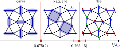
which is represented schematically in Fig. 1. $J_{D}$ is an intra-dimer coupling (denoted by $\langle ij\rangle$) and $J$ a mutually frustrating inter-dimer coupling (denoted $\langle\langle ij\rangle\rangle$). The ground state is clearly a dimer-product phase at small $J/J_{D}$ and a square-lattice antiferromagnet (AF) at large coupling ratios. As intimated above, the ground-state phase diagram is in fact quite well known, with the most quantitatively accurate results provided by the ansatz of infinite projected entangled-pair states (iPEPS, which we will extend here to finite temperatures) Corboz and Mila (2013). As shown in Fig. 1, the singlet dimer-product state is found up to $J/J_{D}=0.675(2)$ and the AF state beyond $J/J_{D}=0.765(15)$, with a gapped, plaquette-based state occurring in the intermediate regime. The lower quantum phase transition (QPT) is of first order; the upper one has also been found numerically to be first-order, but only weakly so Corboz and Mila (2013), and this has also been questioned Lee et al. . Any finite temperature will destroy the magnetic order of the AF phase in this 2D system. By contrast, in the plaquette phase one expects an Ising transition to occur at finite temperatures as the plaquette order, which breaks the lattice symmetry, is lost. In the dimer-product state, no such physics is expected.

Figure 1: Geometry and coupling constants, $J_{D}$ and $J$ (center panel), of the Shastry-Sutherland model [Eq. (1)]. The three panels show schematic representations of the singlet dimer-product state, which is exact, the plaquette state, and the Néel phase. Shaded ellipses and squares denote respectively dimer- and plaquette-singlet states. Phase boundaries are taken from Ref. Corboz and Mila (2013).

Somewhat remarkably, the Shastry-Sutherland model has a faithful realization in the material SrCu₂(BO₃)₂, which has exactly the right geometry and only weak non-Heisenberg (primarily Dzyaloshinskii-Moriya) interactions. Discovered in 1991 Smith and Keszler (1991) and first studied for its magnetic properties 20 years ago this year Kageyama et al. (1999a), SrCu₂(BO₃)₂ lies in the dimer-product phase Miyahara and Ueda (1999) and shows a very flat band of elementary triplet (“triplon”) excitations Kageyama et al. (2000a); Gaulin et al. (2004). Excellent magnetic susceptibility Kageyama et al. (1999a, b) and specific-heat Kageyama et al. (2000b) measurements made at this time were used to estimate the coupling ratio as $J/J_{D}\simeq 0.635$, thereby placing SrCu₂(BO₃)₂ rather close to the dimer-plaquette QPT. Detailed experiments performed in the intervening two decades have revealed a spectacular series of magnetization plateaus Kageyama et al. (1999a); Onizuka et al. (2000); Kodama et al. (2002); Sebastian et al. (2008); Takigawa and Mila (2011); Takigawa et al. (2013); Jaime et al. (2012); Matsuda et al. (2013); Haravifard et al. (2016), as well as a curious redistribution of spectral weight at temperatures very low on the scale of the triplon gap Gaulin et al. (2004); Zayed et al. (2014). Of most interest to our current study is the result Zayed et al. (2017) that an applied pressure makes it possible to increase the ratio $J/J_{D}$ to the extent that, at approximately 1.9 GPa, the material is pushed through the QPT into a plaquette phase. Data for the specific heat under pressure have only appeared Guo et al. concurrently with the present study, and indicate that the low-temperature peak moves to a lower temperature at 1.1 GPa before evidence of an ordered phase appears at 1.8 GPa.

In contrast to the ground state, the excited states and thermodynamics of the Shastry-Sutherland model are not at all well known around the QPT, despite the attention focused on this regime due to SrCu₂(BO₃)₂. Full exact diagonalization (ED) has been limited to systems of up to 20 sites and, as we will demonstrate in detail here, suffer from significant finite-size limitations at $J/J_{D}>0.6$. Quantum Monte Carlo (QMC) methods suffer from extreme sign problems, and despite a recent study by some of us Wessel et al. (2018) that expands the boundaries of what is possible by QMC, the low-temperature behavior in the regime $J/J_{D}>0.6$ remains entirely inaccessible. iPEPS methods work in the thermodynamic limit and are immune to frustration problems, but to date have been limited to ground-state properties. As a consequence, two decades after their measurement, the best interpretation of the thermodynamic properties of SrCu₂(BO₃)₂ Kageyama et al. (1999b, 2000b), and the origin of the estimate $J/J_{D}=0.635$, remain based on ED of 16- and 20-site clusters Miyahara and Ueda (2000, 2003).

Figure 2: (a) Magnetic specific heat, $C(T)$, and (b) magnetic susceptibility, $\chi(T)$, of the Shastry-Sutherland model in the regime of coupling ratios $0.60\leq J/J_{D}\leq 0.66$. The number of sites in the TPQ calculations is $N=36$ and the shaded regions show the standard error of the TPQ method for the respective coupling ratios (Sec. IV). The iPEPS bond dimension is $D=18$.

Here we introduce two qualitative technical advances in numerical methods for computing thermodynamic properties and benchmark them by application to the Shastry-Sutherland model in the dimer-product phase up to the QPT. For a quantum many-body system, a thermal equilibrium state can be represented by a typical pure state, which is known as a thermal pure quantum (TPQ) state Sugiura and Shimizu (2012, 2013). This result can be understood as a consequence of a more general phenomenon, known as quantum typicality Hams and De Raedt (2000); Goldstein et al. (2006). All statistical-mechanical quantities can be obtained from averaging over a few TPQ states. For practical purposes, obtaining TPQ states by ED allows access to thermodynamic quantities without having to perform a full diagonalization, and hence admits a qualitative increase in accessible system sizes Yamaji et al. (2014, 2016). We will exploit TPQ methods to reach system sizes of $N=40$ in the Shastry-Sutherland problem.

iPEPS are a tensor-network ansatz to represent a quantum state on an infinite lattice Verstraete and Cirac ; Jordan et al. (2008); Nishio et al. , here in 2D, whose accuracy is controlled by the bond dimension, $D$, of the tensor. In fact this ansatz provides not only a compact representation for the ground states of gapped local Hamiltonians, but also for representing a purification of the thermal density operator, and hence the thermal states of local Hamiltonians. Here we exploit newly developed algorithms Czarnik et al. (2019) allowing the efficient calculation of imaginary-time evolution processes, which in general require additional truncation to retain the value of $D$ at each time step, to generate thermal states of the Shastry-Sutherland Hamiltonian and hence to compute its thermodynamic properties.

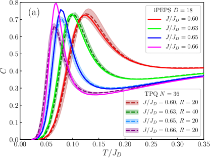
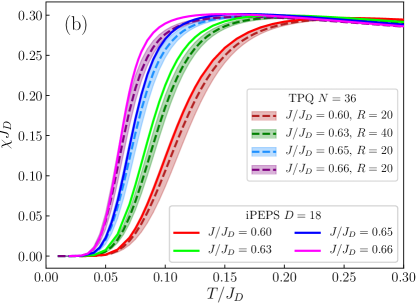
Our TPQ and finite-$T$ iPEPS methods enable us to capture the physics of the Shastry-Sutherland model, and thus of SrCu₂(BO₃)₂, in a way not hitherto possible near the QPT. To illustrate this clearly, in Fig. 2 we show sample results from both methods for the magnetic specific heats and susceptibilities of Shastry-Sutherland models with coupling ratios $J/J_{D}=0.60$, 0.63, 0.65, and 0.66. Over this small range of couplings near the QPT, the specific heat develops a pronounced two-peak form, with a broad higher peak lying just beyond the range of Fig. 2(a). The narrow lower peak, presumably also characteristic of finite-energy excitations in the magnetically disordered dimer-product phase, becomes surprisingly sharp and moves to a remarkably low energy as the QPT is approached. The corresponding susceptibilities rise increasingly abruptly before an increasingly “square” turnover at their maximum. We draw attention to the fact that the results from both our methods are in excellent quantitative agreement, apart from the specific-heat peak heights extremely close to the QPT. These characteristic shapes, and their systematic evolution, have not been obtained before and shed new light both on the thermodynamic quantities themselves and on the underlying excitation spectrum responsible for their form.

The manuscript is organized as follows. In Sec. II we introduce TPQ states and their application to the calculation of thermodynamic quantities. In Sec. III we provide a brief introduction to iPEPS and discuss the generation of thermal states by their imaginary-time evolution. Section IV presents our complete results from both methods for the magnetic specific heat and susceptibility of the Shastry-Sutherland model over the coupling range $0.60\leq J/J_{D}\leq 0.66$, which are summarized in Fig. 2 and which it has not been possible to obtain with any reliability in previous studies. In Sec. V we discuss the physics of the sharp features we observe in the specific heat near the QPT, the limits of our numerical methods in the context of the Shastry-Sutherland model, and the application of our results to the material SrCu₂(BO₃)₂. Section VI contains a brief summary and perspective concerning the impact of our results in frustrated quantum magnetism.

II Thermodynamics from thermal pure quantum states

To evaluate the thermal average of a quantum mechanical observable, $A$, in the canonical ensemble, one computes

$$\langle A\rangle=\operatorname{Tr}({\rm e}^{-\beta H}A)/\mathcal{Z},$$ (2)

where $H$ denotes the Hamiltonian, $\beta=1/(k_{\textrm{B}}T)$ the inverse temperature, $k_{\textrm{B}}$ the Boltzmann constant, and $\mathcal{Z}=\operatorname{Tr}({\rm e}^{-\beta H})$ the canonical partition function. Thermal pure quantum (TPQ) states provide an alternative approach to the evaluation of thermodynamic properties Sugiura and Shimizu (2012, 2013). The trace of any operator, $A$, can be evaluated by taking the average of its expectation values over a set of random vectors,

$$\operatorname{Tr}(A)=d\,\overline{\braket{r}{A}{r}},$$ (3)

where $\ket{r}$ denotes a normalized vector with random normal-distributed components and $d$ denotes the dimension of the Hilbert space. Hence, any thermal average can be estimated by evaluating

$$\langle A\rangle=\frac{\overline{\braket{\beta}{A}{\beta}}}{\overline{\braket{\beta}{\beta}}},$$ (4)

where

$$\ket{\beta}\equiv\textrm{e}^{-\frac{\beta}{2}H}\ket{r}$$ (5)

denotes the “canonical TPQ” state Sugiura and Shimizu (2013) and $\overline{\mbox{\ldots\raisebox{5.69046pt}{}}}$ denotes the average over the random vectors $\ket{r}$. Importantly, the TPQ state, $\ket{\beta}$, is still random. The variance of the estimate in Eq. 4 decreases as $1/\sqrt{d}$, where $d=2^{N}$ for a $S=1/2$ lattice model on $N$ sites, and hence becomes exponentially small as a function of the system size under only mild assumptions about the form of the operator $H$; a precise statement may be found in Ref. Sugiura and Shimizu (2013). For larger system sizes, it is therefore necessary to generate only relatively few random TPQ states, $\ket{\beta}$, in order to achieve small statistical errors. Because the samples in the denominator and the numerator of Eq. 4 are correlated when evaluated from the same set of random vectors, $\ket{r}$, we perform a jackknife analysis Efron and Stein (1981) to estimate the error bars.

The key advantage of using TPQ states, when compared with evaluating statistical averages using the standard formalism of Eq. 2, is that the state $\ket{\beta}$ can be approximated numerically to arbitrary precision without resort to a full diagonalization of the Hamiltonian, $H$. Variants of the TPQ method have been employed in several numerical studies of static and dynamical observables Yamaji et al. (2014, 2016); Steinigeweg et al. (2015, 2016); Shimokawa and Kawamura (2016); Rousochatzakis et al. (2019); Laurell and Okamoto . Whereas Ref. Sugiura and Shimizu (2013) proposed a Taylor-expansion technique, here we improve the speed of convergence by using the Lanczos basis Lanczos (1950) of the Krylov space of $H$ to evaluate the states $\ket{\beta}$.

The $n$th orthonormal basis vector in the Lanczos basis, $\ket{v_{n}}$, is given recursively Allaire and Kaber (2008) by

$$\ket{v_{n}}=\ket{\hat{v}_{n}}/{b_{n}},\text{ with }$$ (6)

$$\ket{\hat{v}_{n}}=H\ket{v_{n-1}}-a_{n-1}\ket{v_{n-1}}-b_{n-1}\ket{v_{n-2}},$$ (7)

where $\ket{v_{1}}=\ket{r}$, $b_{1}=0$, and

$$a_{n}=\braket{v_{n}}{H}{v_{n}},\quad b_{n}=\left\lVert\hat{v}_{n}\right\rVert.$$ (8)

By defining the matrix of Lanczos vectors

$$V_{n}=\left(v_{1}|\dots|v_{n}\right),$$ (9)

the $n$th Lanczos approximation of $H$ can be written as

$$H\approx V_{n}T_{n}V_{n}^{\dagger},$$ (10)

where $T_{n}$ is a tridiagonal matrix given by

$$T_{n}=\begin{pmatrix}a_{1}&b_{2}&0&&\cdots&0\\ b_{2}&a_{2}&b_{3}&0&&\vdots\\ 0&b_{3}&\ddots&&&\\ &&&&\ddots&0\\ \vdots&&&\ddots&a_{n-1}&b_{n}\\ 0&\cdots&&0&b_{n}&a_{n}\\ \end{pmatrix}\!.$$ (11)

We use this approximation to evaluate

$$\begin{split}\braket{\beta}{A}{\beta}&=\braket{r}{\textrm{e}^{-\frac{\beta}{2}H}A\textrm{e}^{-\frac{\beta}{2}H}}{r}\\ &\approx\braket{r}{V_{n}\textrm{e}^{-\frac{\beta}{2}T_{n}}V_{n}^{\dagger}AV_{n}\textrm{e}^{-\frac{\beta}{2}T_{n}}V_{n}^{\dagger}}{r}\\ &=e_{1}\textrm{e}^{-\frac{\beta}{2}T_{n}}V_{n}^{\dagger}AV_{n}\textrm{e}^{-\frac{\beta}{2}T_{n}}e_{1},\end{split}$$ (12)

where $e_{1}=(1,0,\ldots,0)^{\textrm{T}}$. In the case that $A$ is a power of the Hamiltonian, $A=H^{k}$, we have

$$V_{n}^{\dagger}H^{k}V_{n}=T_{n}^{k}.$$ (13)

We stress that the only quantities to be computed are the sequences $a_{n}$ and $b_{n}$. Further, results at all temperatures can be obtained from a single evaluation of the Lanczos basis. The exponentiated tridiagonal matrices, $\textrm{e}^{-\frac{\beta}{2}T_{n}}$, are computed by the eigendecomposition of the matrices $T_{n}$ and exponentiation of the diagonal matrix of eigenvalues. The eigendecomposition of $T_{n}$ is computed using an implicit QR method Demmel (1997); Golub and Van Loan (1996); Parlett (1998) by calling the LAPACK routine dsteqr Anderson et al. (1999); Bai et al. (2000). The dimension, $n$, of the Krylov space is increased until the desired precision is achieved. The computations in this manuscript required a dimension $n<150$ to achieve a precision superior to the statistical errors.

In our computations we use a block-diagonal form of the Hamiltonian,

$$H=\bigoplus_{\rho}H_{\rho},$$ (14)

where the blocks $H_{\rho}$ correspond to the Hamiltonian in different lattice-symmetry and total-$S_{z}$ sectors. Statistical averages are evaluated in each individual block and then summed,

$$\operatorname{Tr}\left({\rm e}^{-\beta H}A\right)=\sum_{\rho}\operatorname{Tr}\left({\rm e}^{-\beta H_{\rho}}A_{\rho}\right).$$ (15)

We employ the techniques proposed in Ref. Wietek and Läuchli (2018) to perform the computations in the individual symmetry sectors.

It has recently become possible to compute Lanczos approximations in particular symmetry sectors for systems of up to $N=50$ $S=1/2$ sites for the Heisenberg model on the square lattice and $N=48$ $S=1/2$ on the kagome lattice Wietek and Läuchli (2018). It is worth noting here that the latter geometry and model are particularly favorable for TPQ Sugiura and Shimizu (2013) because the density of states is high at very low energies Läuchli et al. (2011). However, deriving thermodynamic quantities from the TPQ method requires that these Lanczos approximations be computed multiple times in each symmetry sector for a number, $R$, of random “seeds”, i.e. independent random realizations of the vector $\ket{r}$ in Eq. (5), and it is $R$ that determines the statistical error. Thus restrictions on CPU time currently limit the practical application of the TPQ approach to an upper limit of 40–42 $S=1/2$ spins. More specifically, the calculations in this manuscript were performed with $R=80$ seeds for all coupling ratios $J/J_{D}$ on clusters of $N=32$ spins and $R=20$ for the $N=36$ cluster, except at $J/J_{D}=0.63$, where $R=40$ seeds were evaluated. For the $N=40$ cluster we used $R=5$. In total, the TPQ calculations in this manuscript required approximately 5.5M CPU hours.

We comment that our implementation of the TPQ method is reminiscent of the finite-temperature Lanczos method Jaklič and Prelovšek (1994), which has also recently been pushed to a cluster of $N=42$ $S=1/2$ spins for the kagome lattice Schnack et al. (2018). Although the precise relation between these two different methods remains to be understood, currently we believe that the TPQ approach has a more systematic theoretical foundation and as a consequence that the errors within this approach are better controlled.

For system sizes $N\leq 20$, full diagonalization of the Hamiltonian yields numerically exact results with no statistical errors. An intermediate method is to compute a large number of low-lying eigenstates, for example by using the variant of the Lanczos method outlined in Ref. Honecker and Wessel (2009), and to approximate the low-temperature thermodynamics using these. Despite the significant advantage of also providing results that are entirely free of statistical errors, this method remains restricted by the fact that the required numbers of eigenvalues are large even at the surprisingly low temperatures where the dominant physical processes occur in the present case (Sec. IV). Thus we present benchmarking Lanczos ED results for cluster sizes up to $N=28$, although we comment that $N=32$ would be accessible were we to invest CPU times comparable to those used in our TPQ calculations.

Figure 3: (a) Magnetic specific heat, $C(T)$, and (b) susceptibility, $\chi(T)$, per dimer at coupling ratio $J/J_{D}=0.63$, comparing results obtained from ED and TPQ calculations for system sizes from $N=16$ to 40 sites

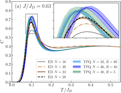
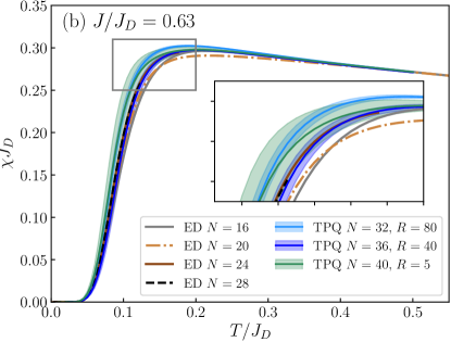
As an illustration of the manner in which TPQ system sizes allow access to the thermodynamic properties of the Shastry-Sutherland model, in Fig. 3(a) we show the specific heat per dimer,

$$C(T)\equiv\frac{2}{N}\,\frac{\partial E}{\partial T}=\frac{2}{N}\,\beta^{2}\left[\braket{H^{2}}-\braket{H}^{2}\right]\!,$$ (16)

where $E\equiv\braket{H}$ is the energy, obtained from our TPQ calculations for coupling ratio $J/J_{D}=0.63$ with $N=32$, 36, and 40. Figure 3(b) shows the corresponding magnetic susceptibility per dimer,

$$\chi(T)\equiv\frac{2}{N}\,\left.\frac{\partial m}{\partial h}\right|_{h=0}=\frac{2}{N}\,\beta\left[\braket{M^{2}}-\braket{M}^{2}\right],$$ (17)

where $h$ is a magnetic field applied along the $z$-axis and $m\equiv\braket{M}$, with

$$M=\sum\limits_{i=1}^{N}S_{i}^{z},$$ (18)

denotes the total magnetization. In both panels of Fig. 3, we compare these TPQ results with ED calculations for systems of sizes $N=16$ and 20, and at low temperatures $N=24$ and 28. The details and context of these results will be discussed in full in Secs. IV and V; for the purposes of this introduction, we stress that both $C(T)$ and $\chi(T)$ have sharp physical features, namely the low-temperature peak in the former and shoulder in the latter, whose shape is manifestly not well reproduced at small $N$ but becomes very much clearer as $N$ is increased. From Fig. 2, this type of access to larger $N$ values becomes increasingly important as the QPT is approached.

III Thermodynamics from iPEPS

An infinite projected entangled-pair state (iPEPS), as a tensor-network ansatz representing a 2D quantum state in the thermodynamic limit Verstraete and Cirac ; Jordan et al. (2008); Nishio et al. , can be seen as a natural generalization of infinite matrix-product states (MPS) to two, or indeed higher, dimensions. While the rank of the tensors used in the representation is determined by the physical problem, the amount of information they contain is determined by their bond dimension, $D$, which is used to control the accuracy of the ansatz. Although iPEPS were introduced originally for representing the ground states of local Hamiltonians, more recently several iPEPS methods have been developed for the representation of thermal states Li et al. (2011); Czarnik et al. (2012); Czarnik and Dziarmaga (2014, 2015a, 2015b); Czarnik et al. (2016a, b, 2017); Dai et al. (2017); Czarnik and Dziarmaga (2018); Kshetrimayum et al. (2019); Czarnik et al. (2019). Here we focus on the approaches discussed in Ref. Czarnik et al. (2019), where an iPEPS is used to represent a purification of the 2D thermal density operator. However, we note that an alternative route to the calculation of finite-temperature properties would be by a direct contraction of the associated (2+1)D tensor network using (higher-order) tensor renormalization-group methods Xie et al. (2012). We comment that MPS-based methods have also been applied recently Bruognolo et al. ; Chen et al. (2018, 2019); Li et al. (2019) to compute the thermal response of finite 2D systems in cylindrical geometries; these approaches provide accurate results for cylinders up to a circumference $W$, which is limited by an exponential increase of the required bond dimension with $W$.

Figure 4: (a) Graphical representation of an iPEPS tensor, $A_{p}^{rtlb}$, in which each leg corresponds to an index of the tensor. The physical index, $p$ (green leg), represents the local Hilbert space of a lattice site (here a dimer) and the other four, $r$, $t$, $l$, and $b$ are auxiliary indices, each with bond dimension $D$, which connect neighboring tensors. (b) A standard iPEPS representing a pure state, shown here for a unit cell containing two different tensors, $A$ and $B$, arranged in a checkerboard pattern on the infinite lattice. A connection between two tensors implies taking the sum over the corresponding index. (c) iPEPS tensor with an extra index, $a$ (blue leg), representing the local Hilbert space of an ancilla site. (d) iPEPS ansatz for the purification, $\ket{\Psi(\beta)}$, of the thermal density operator, $\rho(\beta)$. (e) Representation of $\rho(\beta)=\mathrm{Tr}_{\bf a}\ket{\Psi(\beta)}\bra{\Psi(\beta)}$, where the trace is taken over all ancilla degrees of freedom (shown by the connected blue lines).

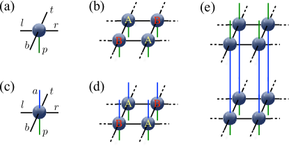
An iPEPS consists of a unit cell of tensors which is repeated periodically on an infinite lattice. For a ground state (pure state), each tensor has one physical index, $p$, describing the local Hilbert space of the dimer and four auxiliary indices, $r$, $t$, $l$, and $b$ [Fig. 4(a)], each with bond dimension $D$, which connect the tensor to its four nearest neighbors on a square lattice. For the Shastry-Sutherland model [Fig. 1] we require one tensor per dimer, arranged in a unit cell with two tensors, A and B, in a checkerboard pattern, as shown in Fig. 4(b).

We represent a thermal density operator, $\rho(\beta)=e^{-\beta\hat{H}}$, at inverse temperature $\beta$ by its “purification,” $\ket{\Psi(\beta)}$, which is a pure state in an enlarged Hilbert space where each physical site, $j$ (here a dimer with local dimension $d=4$), is accompanied by an ancilla site with the same local dimension, described by a local basis $\ket{p,a}_{j}$, where $p$ and $a$ denote respectively the local physical and ancilla basis states. The representation of the thermal state is through its thermal density operator, $\rho(\beta)=\mathrm{Tr}_{\bf a}\ket{\Psi(\beta)}\!\bra{\Psi(\beta)}$, where the trace is taken over all ancilla degrees of freedom, ${\bf a}$. Physically, the ancilla states act as a perfect heat bath, and taking the trace gives exact thermodynamic averages. In tensor-network notation, each ancilla site is incorporated through the additional index $a$ [blue lines in Fig. 4(c)], leading to the diagrammatic representation of $\ket{\Psi(\beta)}$ shown in Fig. 4(d) and of $\rho(\beta)$ in Fig. 4(e) .

At infinite temperature ($\beta=0$), $\ket{\Psi(0)}$ can be represented by the product state, $\ket{\Psi(0)}=\prod_{j}\sum_{k=1}^{d}\ket{k,k}_{j}$ (with bond dimension $D=1$), which for $\rho(0)$ yields the identity operator. The purified state at any given $\beta$ can be obtained as $\ket{\Psi(\beta)}=\hat{U}(\beta/2)\ket{\Psi(0)}$, where the imaginary-time evolution operator $\hat{U}(\beta)=e^{-\beta\hat{H}}$ acts on the physical degrees of freedom of $\ket{\Psi(0)}$. In practice we use a Trotter-Suzuki decomposition of $\hat{U}(\beta)$, meaning it is split into $M$ imaginary-time steps, $\tau=\beta/M$, and approximate the operator for a single time step by a product of nearest-neighbor time-evolution operators, $\hat{U}(\tau)=\prod_{\langle i,j\rangle}\hat{U}_{ij}(\tau)$, with $\hat{U}_{ij}(\tau)=e^{-\tau\hat{H}_{ij}}$, where $\langle i,j\rangle$ denotes all nearest-neighbor site pairs in the unit cell .

Each application of $\hat{U}_{ij}$ increases the bond dimension between the tensors on sites $i$ and $j$ to a larger value, $D^{\prime}>D$, which for reasons of efficiency must be truncated back to $D$ at every step. As in the imaginary-time evolution of ground states, there exist several approaches for the truncation of a bond index, the two most common being the simple- Jiang et al. (2008) and full-update methods Jordan et al. (2008); Corboz et al. (2010). In the simple-update approach, the truncation is performed using a local approximation of the state, which is computationally cheap but does not yield the optimal truncation. In the full-update approach, a bond is truncated in a manner optimal under the method by which the entire state is taken into account; however, this is considerably more computationally expensive and in general it is not possible to reach bond dimensions as large as by the simple-update technique. Below we compare results obtained by these two approaches. Further details concerning the iPEPS ansatz and algorithms for thermal states may be found in Ref. Czarnik et al. (2019).

For contraction of the thermal-state tensor network, which is required to compute all physical expectation values, we use a variant Corboz et al. (2014) of the corner-transfer-matrix (CTM) renormalization-group method Nishino and Okunishi (1996); Orús and Vidal (2009) in which the accuracy is controlled by the boundary bond dimension, $\tilde{\chi}$. To improve the efficiency of the calculations we exploit the global U(1) symmetry Singh et al. (2011); Bauer et al. (2011) of the model of Eq. 1. Further details of the iPEPS methods we employ here may be found in Refs. Corboz et al. (2010); Corboz and Mila (2013); Phien et al. (2015).

Figure 5: Comparison of $D=14$ iPEPS data for (a) the magnetic specific heat and (b) the magnetic susceptibility for the Shastry-Sutherland model with $J/J_{D}=0.63$. The reference line corresponds to a $D=14$ simple-update calculation with time step $\tau=0.04$, boundary bond dimension $\tilde{\chi}=50$, and in panel (b) a field $h/J_{D}=0.01$. For each of the other lines, one parameter has been varied in the calculation with respect to the reference line, as indicated in the legend. The insets magnify the maxima and the minimum.

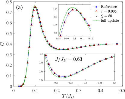
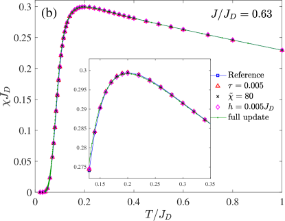
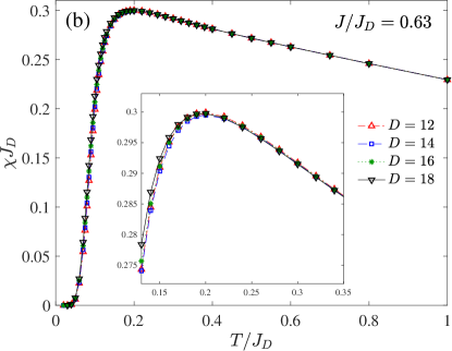
Turning to the evaluation of the thermodynamic properties of the Shastry-Sutherland model with iPEPS, we obtain the magnetic specific heat [Eq. (16)] from the numerical derivative of the energy as a function of the temperature and the magnetic susceptibility [Eq. (17)] from the numerical derivative of the magnetization with respect to a small external magnetic field, $h$. To illustrate the dependence of our results on the parameters $\tau$, $D$, and $\tilde{\chi}$ intrinsic to the iPEPS procedure, in Figs. 5 and 6 we show example data for the coupling ratio $J/J_{D}=0.63$.

Figure 6: iPEPS results for (a) the magnetic specific heat and (b) the magnetic susceptibility of the Shastry-Sutherland model with $J/J_{D}=0.63$, obtained by the simple-update method for different values of the bond dimension, $D$. The insets magnify the maxima and the minimum.

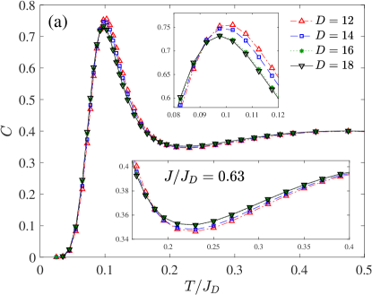
Our primary results are obtained using a second-order Trotter-Suzuki decomposition with a time step $\tau=0.04$. To demonstrate that this value is sufficiently small, meaning that the Trotter discretization error is negligible compared to the finite-$D$ errors (below), in Fig. 5 we show the comparison with results obtained using a time step $\tau=0.005$. Further, it is easy to show that a relatively small boundary bond dimension, such as $\tilde{\chi}=50$ for $D=14$, is large enough for the accurate computation of expectation values. As both panels of Fig. 5 make clear, results obtained using $\tilde{\chi}=80$ are almost identical to $\tilde{\chi}=50$. To compute the magnetic susceptibility we use a field $h/J_{D}=0.01$, which is sufficiently small that the discretization error is not significant; a comparison with $h/J_{D}=0.005$ is shown in Fig. 5(b).

As noted above, the key figure of merit in iPEPS calculations of physical quantities is $D$. Because the “appropriate” value of $D$ to capture the physics of a system varies widely with the problem at hand, we will focus throughout our analysis of the Shastry-Sutherland model on benchmarking our results by comparing $D$ values. To begin the investigation of $D$-dependence, and finite-$D$ convergence, in Fig. 6 we present iPEPS data for $J/J_{D}=0.63$, obtained by the simple-update method for a range of different bond dimensions. We find in Fig. 6(a) that the position of the specific-heat peak shifts slightly ($4\%$) downwards in temperature with increasing $D$, while its height is also reduced ($2\%$). However, these changes take place largely from $D=12$ to $D=16$, whereas changes between the $D=16$ and $D=18$ data are scarcely discernible on the scale of the figure. In the susceptibility [Fig. 6(b)], finite-$D$ effects are clearly very small for $T/J_{D}>0.2$; for $0.05<T/J_{D}<0.2$ a small increase can be observed with increasing $D$.

Finally, to investigate the difference between results by using the simple- and full-update approaches, we return to Fig. 5. At fixed $D=14$, this difference is relatively small in the specific heat, amounting to changes of less than $2\%$ in the position and height of the peak [inset, Fig. 5(a)]. For the susceptibility, differences between the two approaches are minimal [Fig. 5(b)]. Because this difference is small in comparison with the finite-$D$ effects shown in Fig. 6, we focus henceforth on the simple-update approach, which allows us to reach bond dimensions as large as $D=20$ in the present problem, rather than the full-update approach, where $D=14$ represents a practical upper limit.

Figure 7: (a) Magnetic specific heat of the Shastry-Sutherland model at $J/J_{D}=0.50$, computed by TPQ with $N=32$ and 36 and by iPEPS with $D=16$ and 18. Shown for comparison are ED results with $N=20$ and QMC results with $N=32$ and 200. (b) Corresponding magnetic susceptibility.

IV Thermodynamics of the Shastry-Sutherland model with $0.60\leq J/J_{D}\leq 0.66$

We begin the systematic presentation and comparison of our thermodynamic results by making contact with the previous state of the art, as shown in Ref. Wessel et al. (2018). The analysis of these authors, which included ED, QMC, and high-temperature series expansions (HTSEs), terminated at the coupling ratio $J/J_{D}=0.60$, where all three methods were beyond their limits. However, it was shown that QMC remains a highly accurate technique, with only minimal sign problems and thus applicable with large system sizes, for $J/J_{D}<0.526$. Thus we first show, in Fig. 7, the magnetic specific heat and susceptibility for $J/J_{D}=0.50$ computed by TPQ for system sizes $N=32$ and 36 and by iPEPS with $D=16$ and 18. By comparison with the large-system QMC benchmark ($N=200$ sites), we observe that our iPEPS data, arguably a product of the newest and least well-characterized technique, agree precisely for both bond dimensions shown.

For ED-based methods, it was known already Wessel et al. (2018) that clusters of size $N=20$ give an adequate account of the thermodynamics at this coupling ratio, with the exception of the very peak in $C(T)$ [Fig. 7(a)]. Nevertheless, our TPQ results contain two surprises, in the form of the rather large errors and the significant difference between results for the two cluster sizes. Regarding how accurately TPQ reproduces both $C(T)$ and $\chi(T)$ at temperatures around the $C(T)$ peak, we note that our $N=32$ results do indeed lie close to the QMC benchmark for this system size, with the discrepancy being well within the error tube. Quite generally, the origin of these somewhat large errors lies in the very low density of low-lying states in the spectrum, as pointed out in Ref. Sugiura and Shimizu (2013), and this is certainly the case in the Shastry-Sutherland model when the gap is as large as its value at $J/J_{D}=0.5$ (more details may be found in Sec. VA). We will show that our TPQ results become progressively more accurate as the system approaches the QPT, which reduces the gap, until coupling ratios very close to the transition. With regard to the effects of the shape or geometry of the cluster, regrettably the method allows little control beyond the absolute value of $N$.

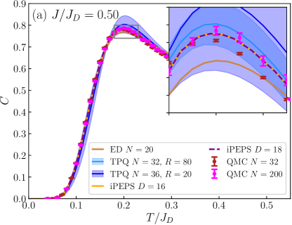
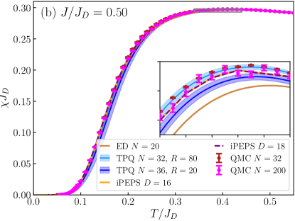
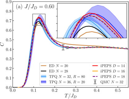
In Fig. 8 we move into the previously intractable parameter regime by showing the specific heat and susceptibility at $J/J_{D}=0.60$ computed by TPQ for system sizes $N=32$ and 36 and by iPEPS with $D=14$, 16, and 18. Focusing first on the specific heat [Fig. 8(a)], we still observe a single peak at low temperatures ($T/J_{D}\simeq 0.12$), but followed by a very flat plateau extending to $T/J_{D}\simeq 0.45$. It is clear that our TPQ results, augmented by an ED calculation with $N=28$ reaching temperatures just above the peak, exhibit finite-size effects in this region. Both the position and the sharpness of the peak show a significant evolution as the system size is augmented, although from $N=32$ to 36 the difference is within the error bars of the method. As expected from Sec. III, the three iPEPS bond dimensions show good convergence, in fact to a peak shape exactly between the two TPQ estimates. Outside the peak region, all methods and sizes agree extremely well, and also converge at high temperatures to the values obtained by QMC, which returns results of acceptably low statistical uncertainty at $T/J_{D}\gtrsim 0.25$ for this coupling ratio Wessel et al. (2018).

Figure 8: (a) Magnetic specific heat of the Shastry-Sutherland model at $J/J_{D}=0.60$, computed by TPQ with $N=32$ and 36 and by iPEPS with $D=14$, 16, and 18. Shown for comparison are ED results with $N=20$ and with $N=28$ at temperatures $T/J_{D}\leq 0.14$, as well as QMC results with $N=32$ from Ref. Wessel et al. (2018). (b) Corresponding magnetic susceptibility.

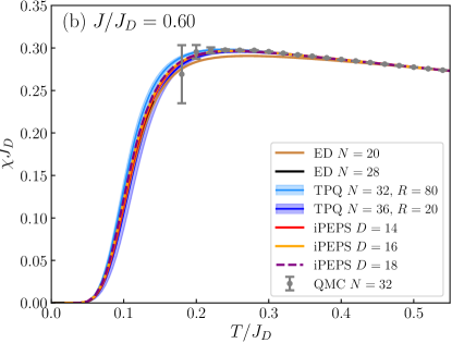
The corresponding susceptibility [Fig. 8(b)] is less sensitive to differences in either system size or bond dimension. Indeed, only an ED calculation with $N=20$ is not capable of capturing the maximum of $\chi(T)$ for this coupling ratio. However, the two TPQ results do differ concerning the exact location in temperature of the rapid rise in $\chi(T)$, and the fully convergent iPEPS results appear to offer the benchmark. All of our calculations agree closely on the location of the broad maximum. We comment that the characteristic temperature of $\chi(T)$ need not match that of $C(T)$, given that the former has contributions only from magnetic states but the latter includes the contributions of singlets. However, at this coupling ratio, where the one-triplon excitations of the system lie below all two-triplon bound states Wessel et al. (2018), the peak in $C(T)$ and the rise of $\chi(T)$ do indeed coincide. We discuss the excitation spectrum of the model in detail in Sec. VA.

Figure 9: (a) Magnetic specific heat of the Shastry-Sutherland model at $J/J_{D}=0.63$, computed by TPQ with $N=32$, 36, and 40 and by iPEPS with $D=14$, 16, and 18. Shown for comparison are ED results with $N=20$ and with $N=28$ at temperatures $T/J_{D}\leq 0.125$, as well as QMC results with $N=32$. (b) Corresponding magnetic susceptibility.

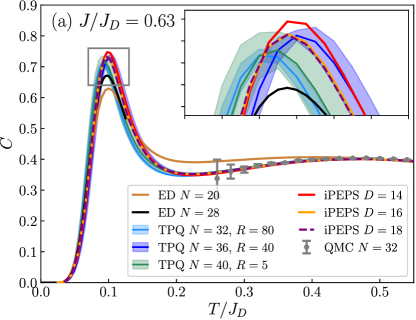
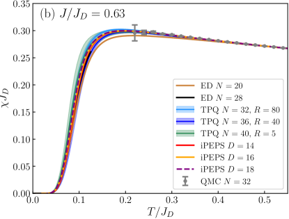
As noted in Sec. I, the coupling ratio $J/J_{D}=0.63$ has special significance in the Shastry-Sutherland model because of its proposed connection to the material SrCu₂(BO₃)₂, and for this reason we have already used it for benchmarking purposes in Secs. II and III. In Fig. 9 we compare our TPQ and iPEPS results for $C(T)$ and $\chi(T)$. Independent of either method, we observe that the specific-heat peak has become sharper, although not any taller, and that the drop on its high-$T$ side has turned into a true minimum, before $C(T)$ recovers to a broad maximum around $T/J_{D}=0.45$. The position of the sharp peak has moved down to $T/J_{D}\simeq 0.10$, which is a remarkably large shift for such a small change in coupling ratio. Although the corresponding features are far less pronounced in $\chi(T)$, it it clear that onset is considerably steeper than at $J/J_{D}=0.60$ and that the temperature scales both for it and for the flat maximum are lower.

Focusing on the details of $C(T)$ [Fig. 9(a)], once again our TPQ results for $N=32$ and 36, particularly in combination with $N=28$ ED, show nontrivial changes around the peak, both in its position and its height. However, the $N=40$ data appear to offer a systematic interpolation of both quantities. In our iPEPS results, $D=14$ no longer appears representative of the large-$D$ limit at this coupling ratio, but finite-$D$ effects seem to become very small at higher $D$. Qualitatively, our optimal iPEPS peak appears to be very close to the form at which one might expect the TPQ results to converge with system size, and we will quantify this statement below. In $\chi(T)$ [Fig. 9(b)], the two methods achieve full convergence for all $N$ and $D$, despite the lowering effective temperature scales, and we draw attention to the fact that previous ED and QMC studies at this coupling ratio could not capture this low-temperature behavior with any accuracy; we revisit this point in the context of SrCu₂(BO₃)₂ in Sec. VC.

Figure 10: (a) Magnetic specific heat of the Shastry-Sutherland model at $J/J_{D}=0.65$, computed by TPQ with $N=32$ and 36 and by iPEPS with $D=14$, 16, and 18. Shown for comparison are ED results with $N=20$ and with $N=28$ at temperatures $T/J_{D}\leq 0.11$, as well as QMC results with $N=32$. (b) Corresponding magnetic susceptibility.

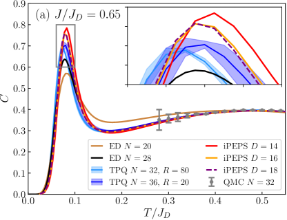
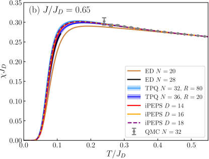
Proceeding yet closer to the QPT, Fig. 10 shows the specific heat and susceptibility at the coupling ratio $J/J_{D}=0.65$. Clearly the “peak-dip-hump” shape of $C(T)$ has become significantly more pronounced in all respects than at $J/J_{D}=0.63$; the peak is sharper, the dip is deeper, and the separation of the peak and the broad hump has increased, with the peak moving below $T/J_{D}=0.09$ and the high-$T$ maximum centered around $T/J_{D}=0.5$. Once again the progression from our ED data at $N=28$ to TPQ with $N=32$ and then 36 shows an increasing ability to capture the tip of the peak, but it cannot be said that convergence has been reached [inset, Fig. 10(a)]. As at $J/J_{D}=0.63$, our iPEPS data for $D=16$ and 18 are in essence indistinguishable and do suggest the peak to which the TPQ results are converging. At all other parts of the $C(T)$ curve, convergence is complete by all methods. In the corresponding susceptibility, again the ED and TPQ size sequence provides a systematic convergence towards the “squareness” of the turnover from rapid rise to broad maximum, while the higher iPEPS bond dimensions have converged to the shape of this feature.

Figure 11: (a) Magnetic specific heat of the Shastry-Sutherland model at $J/J_{D}=0.66$, computed by TPQ with $N=32$ and 36 and by iPEPS with $D=14$, 16, and 18. Shown for comparison are ED results with $N=20$ and with $N=28$ at temperatures $T/J_{D}\leq 0.10$. (b) Corresponding magnetic susceptibility.

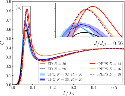
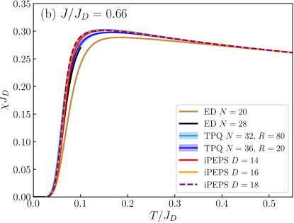
We take the coupling ratio $J/J_{D}=0.66$, shown in Fig. 11, as the upper limit to the validity of comparing our methods. Physically, it is obvious that the peak-dip-hump shape of $C(T)$ becomes yet more pronounced, that the dip is deeper, and that the peak is even lower-lying and sharper than at $J/J_{D}=0.65$ [Fig. 11(a)]. Numerically, it appears that both our methods show slower convergence, not only around the peak but also in the dip. In more detail, our $N=32$ and 36 TPQ results, and our $D=16$ and 18 iPEPS results, do both offer internally consistent peak shapes. However, it is no longer clear that TPQ and iPEPS might extrapolate to the same limit, although this could be because the effective location of the QPT differs for the two methods due to finite-$D$ and -$N$ corrections, implying closer proximity to a competing phase in one than in the other. On the overall shape of $C(T)$, we comment that the hump can be understood as the energy scale of local spin-flipping processes on the scale of $J_{D}$, while the low-$T$ peak is the focus of our discussions in Sec. VA. Concluding with the susceptibility at $J/J_{D}=0.66$ [Fig. 11(b)], again our iPEPS results offer a consistent picture of the very steep onset and square maximum, while our TPQ results suggest better agreement with iPEPS at $N=32$ than at $N=36$.

The results in Figs. 8 to 11 capture the thermodynamic properties of the Shastry-Sutherland model with a degree of precision that was entirely unattainable by all previous techniques. It is safe to say that no prior numerical studies had even identified the peak-dip-hump form of the purely magnetic specific heat with any reliability, let alone given an indication of how narrow the low-$T$ peak becomes in the regime near the QPT. While the square shape of $\chi(T)$ has been known since the early measurements on SrCu₂(BO₃)₂ Kageyama et al. (1999a, b), again no numerical approaches had reproduced this form. We discuss both the physics underlying these features and the experimental comparison in Sec. V.

The thermodynamic properties of the Shastry-Sutherland model nevertheless set an extremely challenging problem in the regime close to the QPT, even in the dimer-product phase where the ground state is exact and no finite-temperature transition is expected. It is clear in Figs. 8 to 11 that neither our TPQ nor our iPEPS calculations can be judged to be fully convergent, and thus accurate, as $J/J_{D}$ approaches the presumed critical value of 0.675. Because both are limited by their control parameters, $N$ for TPQ and $D$ for iPEPS, an optimal reproduction of the exact thermodynamics would be obtained by extrapolating both sets of results to infinite $N$ or $D$.

Figure 12: Characteristic position and height of the low-$T$ peak in the magnetic specific heat of the Shastry-Sutherland model, shown for our ED and TPQ results as functions of $1/N$ and for our iPEPS results as functions of $1/D$. (a,b) $J/J_{D}=0.60$. (c,d) $J/J_{D}=0.63$. (e,f) $J/J_{D}=0.65$. (g,h) $J/J_{D}=0.66$.

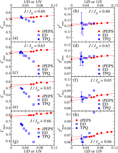
By inspection of the full peak shape in $C(T)$, our TPQ results can only be said to have reached convergence at $N\leq 40$ for $J/J_{D}\leq 0.63$. Similarly, it is not clear that our iPEPS results for the largest available $D$ values (we have performed calculations with $D=18$ at all temperatures and with $D=20$ for temperatures around the peak) can be said to have converged to the shape of the peak at $J/J_{D}=0.66$. For extrapolation purposes, we first extract the primary characteristic features of this low-$T$ peak, namely its position and height. In Fig. 12 we show the convergence of both quantities as functions respectively of $1/N$ in our ED and TPQ calculations and of $1/D$ in our iPEPS calculations, for each of the coupling ratios $J/J_{D}=0.60$, 0.63, 0.65, and 0.66.

Focusing first on our iPEPS results, it is evident that the values we have obtained for both the position and the height of the $C(T)$ peak show an excellent linear convergence with $1/D$ for all coupling ratios. Both quantities decrease with increasing $D$ and in fact their slopes are remarkably insensitive to $J/J_{D}$. Thus we estimate the putative infinite-$D$ limit of the peak characteristics (shown by a filled triangle) by linear extrapolation in $1/D$ and we take the difference of this limit from the result at the largest computed $D$ value as an estimate of the (one-sided) error bar. While all of the iPEPS estimates decrease monotonically with increasing $D$, in the large-$D$ limit one does anticipate exponential convergence in $D$ rather than linear convergence in $1/D$. Thus we expect the true $D=\infty$ limit to lie within the interval indicated by the error bar.

Turning to the ED and TPQ results in Fig. 12, the peak heights at all coupling ratios show a quite systematic convergence, from below and with changing slopes, towards values fully consistent with our iPEPS estimates. By contrast, the finite-size evolution of the peak positions is less clear, but it is true to state for every coupling ratio that their values for all system sizes are either clustered closely around the extrapolated iPEPS values or are trending towards these.

Thus we may conclude that our TPQ and iPEPS results are consistent and convergent for even the most challenging features of the most challenging region of the Shastry-Sutherland phase diagram. As such they may be used as a reliable statement of the excitation spectrum as a function of the coupling ratio, which is the topic of Sec. VA. We discuss the implications of the convergence details in Fig. 12 for future numerical development in Sec. VB.

V Discussion

V.1 Spectrum of the Shastry-Sutherland Model

In Fig. 2(a) we showed our collected results for the specific heat of the Shastry-Sutherland model across the range of coupling ratios $0.60\leq J/J_{D}\leq 0.66$. As the system approaches the QPT from the dimer-product to the plaquette state, one observes the systematic emergence of a narrow low-energy peak, followed at higher temperatures by a deepening dip before a second broad maximum on the scale of $J_{D}/2$. The energy scale of the concentration of low-lying states contributing to the peak falls steeply as the QPT is approached. From the corresponding susceptibilities, shown in Fig. 2(b), it is clear that the decreasing energy scale is largely similar for triplet (and higher spinful) excitations, and hence at minimum that it is not a special property of singlets; the physics of the approach to the QPT seems to affect all excitations in the same general manner.

Figure 13: (a) Position, $T_{\max}^{C}$, and (b) height, $C_{\max}$, of the peak in the specific heat of the Shastry-Sutherland model in the regime of coupling ratios $0.50\leq J/J_{D}\leq 0.66$, as determined from our ED, TPQ, and iPEPS calculations. Also shown in panel (a) is the half-height, $T_{1/2}^{C}$, on the low side of the peak, from which one may deduce an effective peak width (shaded grey region). iPEPS error-bar conventions are as in Fig. 12. At $J/J_{D}=0.50$ we compare in addition with the large-$N$ QMC result. Shown for reference in panel (a) is the function $c\,\Delta_{\rm m}(J/J_{D})$, where $\Delta_{\rm m}={\rm min}[\Delta_{S},\Delta_{T}]$, with $\Delta_{S}$ and $\Delta_{T}$ respectively the gaps of the lowest singlet and triplet excitations obtained for a system of size $N=36$, is the minimal gap in the system; the constant of proportionality is $c=0.28$. (c) Positions of the peak, $T_{\max}^{\chi}$, and of the half-height, $T_{1/2}^{\chi}$, in the susceptibility of the Shastry-Sutherland model in the same range of coupling ratios. Again the shaded region may be considered as an effective width. Shown for reference is the function $d\,\Delta_{T}$, again obtained for $N=36$, with constant of proportionality $d=0.22$.

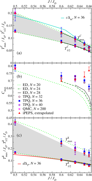
Before discussing the nature of the low-lying spectrum, we characterize the height and temperature scale of the specific-heat peak, and the temperature scale of the susceptibility onset, as the coupling ratio approaches the QPT. The peak position, $T_{\max}^{C}$, shown in Fig. 13(a), clearly falls faster than linearly in $J/J_{D}$, but does not approach zero at the QPT. Based on the expectation that the peak position as a function of $J/J_{D}$ should follow the gap, $\Delta_{\rm m}$, of the system, in Fig. 13(a) we show this quantity based on ED data from the $N=36$ cluster Wessel et al. (2018), and with a multiplicative prefactor of 0.28. The fact that these falling energy scales do not vanish at the QPT is consistent with the first-order nature of this transition Corboz and Mila (2013). The behavior of the peak height [Fig. 13(b)] is less evident, in that it falls on approach to the QPT in our TPQ calculations but increases in our iPEPS ones, the rate of change accelerating with $J/J_{D}$ in both cases. Given the strong finite-size effects visible in our ED and TPQ calculations for $J/J_{D}>0.63$ [Fig. 12], here it appears that our iPEPS results are more representative of the large-$N$ limit. The final piece of information one may wish to extract about the peak is its width, for which we show in addition the temperature $T_{1/2}^{C}$, at which the specific heat attains half its peak height [Fig. 13(a)]; because of the dip and hump on the high-$T$ side, we focus only on the low-$T$ side. We obtain a characteristic width from the quantity $T_{\max}^{C}-T_{1/2}^{C}$, shown as the shaded grey region. We observe that the half-height and full-height positions, and hence the width, scale to a good approximation in the same way with $J/J_{D}$, separated only by constant factors, and conclude that all the peak shapes are actually self-similar on the low-temperature side, with only one characteristic $J/J_{D}$-dependent energy scale.

Figure 14: Low-lying energy spectrum of the Shastry-Sutherland model in the $S=0$ and $S=1$ sectors, computed by ED using clusters of sizes $N=28$ (to ${\tilde{E}}=2.6J_{D}$), $N=24$ (to $3.75J_{D}$), and $N=20$ (to $4.2J_{D}$) and shown over the full range of coupling ratios, $J/J_{D}$, in the dimer-product phase. The excitation energy is denoted by ${\tilde{E}}=E-E_{\rm GS}$, where $E_{\rm GS}$ is the energy of the ground state. The shading represents regions with discrete but dense singlet (blue) and triplet excitations (pink). The lowest pink line shows the one-triplon sector, whose lower edge is $\Delta_{T}(J/J_{D})$; the yellow line shows the two-triplon scattering threshold, $2\Delta_{T}(J/J_{D})$. The lower edge of the lower blue sector, which consists of singlet bound states of two triplons, is $\Delta_{S}(J/J_{D})$. We draw attention to how few states in the three-triplon sector fall below the green line ($\Delta_{S}+\Delta_{T}$) and in the four-triplon sector below the black line ($2\Delta_{S}$).

Because the maximum of $\chi(T)$ is broad and flat, for an accurate characterization of the susceptibility we focus not on its position ($T_{\rm max}^{\chi}$) but on the temperature, $T_{1/2}^{\chi}$ Honecker et al. (2016a), at which $\chi(T)$ reaches half its maximum value during its rapid onset. Both quantities are shown in Fig. 13(c), which indeed confirms significantly larger uncertainties in $T_{\rm max}^{\chi}$ than in $T_{1/2}^{\chi}$. $T_{1/2}^{\chi}$ tracks both $T_{\max}^{C}$ and $T_{1/2}^{C}$ rather closely throughout the range of Fig. 13, albeit with a slightly slower decline very near the QPT. In this sense it functions as a comparable diagnostic of the falling energy scale in the system. Following the expectation that $\chi(T)$ depends on the gap to spinful excitations, in Fig. 13(c) we compare this scale with the triplet gap, $\Delta_{T}(J/J_{D})$, finding a constant of proportionality of approximately 0.22.

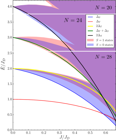
Figure 13 is a very specific diagnostic for the nature of the spectrum of low-lying energy levels, reflecting in particular a large number of states that become more nearly degenerate and are characterized by an ever-smaller (but always finite) gap as the system approaches the QPT. In Ref. Wessel et al. (2018) we showed a schematic illustration of the energy spectrum of the Shastry-Sutherland model as a function of the coupling ratio $J/J_{D}$, based on Lanczos ED calculations to obtain the lowest levels of a cluster of size $N=36$ sites. For more specific insight into the nature of the states revealed by the Lanczos procedure, here we have computed a much larger number of low-energy states, but for smaller clusters (of sizes up to $N=28$). In Fig. 14 we gather these results to show the low-lying spectrum of the system in the $S=0$ and $S=1$ sectors over the full range of coupling ratios. We stress that, given the large number of states in these calculations, it is not easy to observe the discrete structure of the spectrum even in its lowest-lying regions, and as in Ref. Wessel et al. (2018) we use shading to indicate the support of these excitations.

In Fig. 14, the thin red line at the bottom of the triplet spectrum is the elementary “triplon” excitation, which has energy ${\tilde{E}}=J_{D}$ at $J=0$ and remains extremely narrow (non-dispersive) throughout the dimer-product phase due to the perfect frustration (Fig. 1). It is clear that significant numbers of two- and other multi-triplon states, in both the spin sectors shown, move to very low energies as the system approaches the QPT. Because the lowest states in the singlet sector must be of two-triplon origin, and these cross below the one-triplon energy around $J/J_{D}=0.60$ (the exact value depends on $N$), it is equally clear that the physics of the Shastry-Sutherland model in the regime near the QPT is dominated by states one may classify as “strongly bound.” To specify the meaning of this term, the yellow line shows the quantity $2\Delta_{T}(J/J_{D})$, i.e. twice the single-particle gap, which corresponds to the two-triplon scattering threshold, and near the QPT many states lie significantly below this energy. We comment that the separate “families” of excitations that can be traced back to independent two-triplon states at energy ${\tilde{E}}=2J_{D}$ at $J=0$, and similarly for higher triplon numbers [Fig. 14], exhibit a much larger dispersion across the Brillouin zone than do the one-triplon states, due to the smaller effects of geometric frustration on the propagation of bound states Knetter et al. (2000); Totsuka et al. (2001); Miyahara and Ueda (2003). Although some authors have performed perturbative studies of the lowest-lying bound states of the Shastry-Sutherland model Knetter et al. (2000), we are not aware of previous attempts to count them systematically for comparison with thermodynamic properties, as we do next.

Figure 15: Numbers of low-lying singlet and triplet states on an $N=28$ lattice, shown as functions of $J/J_{D}$ in the dimer-product phase. Symbols show ED data while connecting lines are guides to the eye. The horizontal green line shows the number of independent two-triplon scattering states.

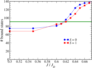
Beyond illustrating significant binding-energy effects in the two- and higher-triplon sectors, Fig. 14 does not provide further information about the structure of the spectrum. As a step in this direction, Fig. 15 shows the numbers of singlet and triplet states lying below the threshold given by the yellow line in Fig. 14. The number of triplet states excludes the $N/2$ states of the one-triplon band. For comparison, the expected number of two-triplon scattering states, ${\textstyle\frac{1}{4}}N({\textstyle\frac{1}{2}}N-1)$, is shown by the green line. Clearly the numbers of “bound” states in both sectors are significant fractions of the number of scattering states throughout the region $J/J_{D}\lesssim 0.55$. Further, the number of $S=1$ states is comparable to that in the $S=0$ sector, despite the fact that the energy gain is greater in the latter. As the QPT is approached, specifically once $J/J_{D}>0.62$ for $N=28$ [Fig. 15], the numbers of low-lying states in both sectors increase well beyond the number of independent two-triplon states.

Figure 16: Total number of excited states lying below the energy $\tilde{E}$ at coupling ratios (a) $J/J_{D}=0.60$, (b) $J/J_{D}=0.63$, and (c) $J/J_{D}=0.66$. Blue lines indicate $S=0$ excitations, red lines $S=1$. Increasing line widths indicate increasing system sizes, $N$, on which ED calculations were performed. Vertical green lines denote the two-triplon scattering thresholds for the corresponding system sizes.

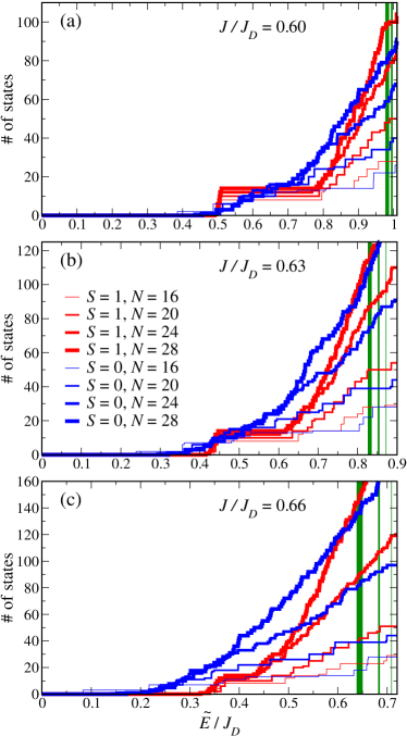
Before discussing the nature of these states, for further information about the low-lying spectra we show in Fig. 16 the total numbers of singlet (blue) and of triplet states (red) lying below a given energy, ${\tilde{E}}$, in ED calculations performed with four different system sizes for three fixed values of $J/J_{D}$ in the interval near the QPT. Here the $N/2$ one-triplon excitations are included in the triplet count, appearing as the plateau region in all the red lines directly above their onset. We note that all excitations with higher spin, $S\geq 2$, lie above the two-triplon scattering threshold for all $J/J_{D}$ values shown; while binding effects have also been observed in the $S=2$ sector Corboz and Mila (2014), these are extremely small and are not detectable in clusters up to $N=28$ due to finite-size effects.

The evolution of this spectrum as a function of the coupling ratio contains two new messages beyond the ever-increasing number of very low-lying states shown in Fig. 15. First, the steadily decreasing gap in the one-triplon sector can be expected to control the response to $\Delta S\neq 0$ processes over most of regime $0.60\leq J/J_{D}\leq 0.66$, but very near the QPT it is overwhelmed by the high density of other triplet states that finally fall to this gap. Second, the dominant feature of the spectrum in this regime is the large number of low-lying singlet states, which are governed by an energy scale that in turn falls significantly more quickly with $J/J_{D}$ than the triplet gap.

To discuss the nature of these states, and hence the consequences of our calculated spectra for the thermodynamic response functions computed in Sec. IV, it is helpful to compare and contrast the Shastry-Sutherland model with the fully frustrated two-leg spin ladder. In this 1D model, some of us Honecker et al. (2016b, a) also found a striking thermodynamic response at low temperatures, which could be traced to a proliferation of low-energy multi-magnon bound states upon approaching a first-order QPT. While it is clear that the proliferation of low-lying states is the origin of the low-temperature properties of the Shastry-Sutherland model, there are some important differences between the 1D and 2D systems, most notably concerning the mechanism behind the formation of these states.

First, in the fully frustrated two-leg ladder, it was clear that these states were truly bound, meaning that they were intrinsic combinations of $n$ contributing triplons, with $n\geq 2$ becoming very large near the QPT. By contrast, in the Shastry-Sutherland system one may identify essentially all of the additional low-lying states, whose origin clearly lies in $n\geq 3$ triplons, with the expected scattering states of two singlet two-triplon bound states or of a singlet bound state and an elementary triplon. It is self-evident that when the energy of a singlet bound state of two triplons falls beyond the one-triplon gap, the lowest-lying scattering states of a pair of singlet bound states must fall below the two-triplon scattering threshold in the $S=0$ sector, shown by the black line in Fig. 14, and so does the scattering state of a singlet bound state and an elementary triplon in the $S=1$ sector, shown by the green line in the same figure. Thus the proliferation of low-lying excitations in the regime $J/J_{D}>0.6$ can, due to the differences in state-counting in 2D, be driven (almost) completely by the strength of the two-triplon binding effect in the singlet sector. It is for this reason that we do not refer to all of the low-lying states we observe here as “bound states.” Concerning the possibility of true multi-triplon binding effects, as noted above we may comment only that, if present, these are sufficiently weak that we are unable to detect them.

Second, at the QPT in the fully frustrated ladder, the bound states cluster strongly at a single energy value of approximately 85% of the one-triplon gap Honecker et al. (2016b, a), but in the Shastry-Sutherland model we observe no such sharp structures in the density of states. Specifically, although we find for $J/J_{D}=0.66$ that low-lying singlet states far outnumber the triplets at any energy $\tilde{E}<0.5J_{D}$ [Fig. 16(c)], there is no sign of a discrete set of degenerate levels, at any energy, that could be related directly to the specific-heat peak. Instead the number of excited states continues to rise with ${\tilde{E}}$, in fact at an increasing rate, such that some very high densities of states may be found at energies of order $0.5J_{D}$ above the lowest ones in each panel of Fig. 16. The distinguishing feature of these broadly distributed states, at least in the singlet sector, is that their binding effects are energetically stronger than in the 1D system. Although finite-size effects prevent us from reaching the QPT ($J/J_{D}=0.675$), at $J/J_{D}=0.66$ the singlet two-triplon bound states have already descended to only 54% of the one-triplon gap (on the $N=28$ cluster). Thus the low-temperature peak in $C(T)$ observed in Sec. IV emerges at a relatively lower energy scale than in the fully frustrated ladder. Certainly the possibility of ascribing our results to only one energy scale is consistent with our discovery in Fig. 13(a) that the peak shapes are identical. In this regard, the strikingly narrow specific-heat peaks near the QPT are not in fact anomalous, in that their relative width is constant and their appearance is a consequence of this one decreasing energy scale. Regarding the susceptibility, the decrease of the one-triplon energy scale in Fig. 16 appears to provide a reasonable account of the decrease in the “onset” temperature indicator $T_{1/2}^{\chi}$ [Fig. 13(c)] over the entire range of $J/J_{D}$, while the steep fall in energy of the other low-lying triplet states may be responsible for the increasingly abrupt (“square”) turnover at the maximum in $\chi(T)$.

In summary, our detailed ED investigation of the low-energy spectrum [Figs. 14, 15, and 16] reveals the rapid descent in energy of a multitude of singlet and triplet states as the QPT is approached. Despite the narrow nature of the $C(T)$ peak, these states do not converge to a single characteristic energy in either sector. In contrast to the $n$-triplon bound states of the fully frustrated ladder near its QPT, the energetics of the low-lying states of the Shastry-Sutherland model are dominated by the binding energy of two triplons into a net singlet. Because this local bound state involves two neighboring orthogonal dimers Knetter et al. (2000); Totsuka et al. (2001), it has little or no relation with the plaquette singlets that control the physics on the other side of the QPT (Fig. 1), and hence one may conclude that the first-order transition involves a complete rearrangement of spin correlations in the system.

V.2 Numerical Methods

We comment only briefly on the limitations and prospects for improvement of our numerical techniques. In a sense the Shastry-Sutherland model near the QPT presents an ideal test-bed for any method, in that the low-$T$ peak in the specific heat becomes progressively narrower, and thus more challenging to reproduce, as the QPT is approached. In our ED and TPQ calculations, it is both clear and completely unsurprising that larger cluster sizes improve the ability of both methods to capture this peak (and the corresponding susceptibility shoulder). Whereas the thermodynamic response at coupling ratio $J/J_{D}=0.60$ could not be reproduced with complete accuracy by $N=20$ ED, or indeed $N=28$ Lanczos ED (Fig. 8), we may assert that $J/J_{D}=0.63$ can be treated accurately by TPQ with $N\leq 40$ (Fig. 9).

However, the limits to TPQ appear to be reached at $J/J_{D}>0.65$, where our calculations are no longer able to capture the anomalously narrow $C(T)$ peak that forms in this regime (Fig. 11). With reference to our discussion of Sec. VA, one may only speculate that the physics of this peak resides in scattering states of the singlet two-triplon bound states whose fully developed real-space extent begins to exceed this cluster size very close to the QPT. As noted in Sec. II, reaching larger cluster sizes with acceptable statistical errors is not possible with present computing power. Similarly TPQ, like ED, is not limited by algorithmic complexity, and indeed our present calculations already exploit all available spin and spatial (cluster) symmetries, implying that more complex Hamiltonians would be subject to stricter limits on $N$.

By contrast, our iPEPS calculations have relatively modest CPU and memory requirements. To date they have been run only on a single node, and thus larger-scale computations would certainly become feasible through the future development of a highly parallelized code. In comparison with more mature numerical methods, tensor-network calculations remain in their relative infancy, and as a result retain significant scope for algorithmic improvement. In current implementations, both CPU and memory requirements increase as high powers of the bond dimension, $D$; although most developments focus on reducing these exponents, it is not proven beyond doubt that large $D$ is the only route to an accurate tensor-network description. As one example, we comment that higher accuracies can be achieved for the same $D$ value within our present calculations by the use of disentangling gates acting on the ancillas Hauschild et al. (2018); Czarnik et al. (2019).

Nevertheless, as demonstrated in Sec. III, the influence of the other variables in the iPEPS method (Trotter step, CTM boundary bond dimension, type of update) is small in comparison with the effects of $D$. Physically, there is at present no known means of relating $D$ as a figure of merit in finite-$T$ (i.e. thermal-state purification) iPEPS implementations with $D$ in a ground-state iPEPS calculation. As with the problem of which absolute value of $D$ is able to capture the physics of any given Hamiltonian (Sec. III), the most reliable approach to date is the empirical one of increasing $D$ and monitoring changes and convergence. As we have shown in Secs. III and IV (Fig. 12), for the present problem we have indeed reached a well-defined limiting regime of $D$, even at $J/J_{D}=0.66$. Thus one may conclude that the Shastry-Sutherland model does not present a physical system where calculations are limited by the ability to capture long-ranged entanglement, as may perhaps be expected when the ground state is a product state, all the excitations are gapped, and the nearby QPT is first-order.

V.3 Experiment

In the light of the data and insight obtained from applying our two advanced numerical methods to the thermodynamics of the Shastry-Sutherland model, we revisit the experimental situation in SrCu₂(BO₃)₂. We note that low-lying singlet excitations in SrCu₂(BO₃)₂ were documented by Raman scattering soon after the discovery of the material Lemmens et al. (2000), and later that the same method was used to study the low-lying spectrum in an applied magnetic field Gozar et al. (2005). The triplet excitations were studied at first by electron spin resonance (ESR) Nojiri et al. (1999) and inelastic neutron scattering Kageyama et al. (2000a). Subsequent high-field ESR measurements were used to demonstrate the presence of two-triplon bound states Nojiri et al. (2003), while a recent application of modern neutron spectroscopy instrumentation studied the lowest bound triplet mode, and its response in a magnetic field, in unprecedented detail McClarty et al. (2017). The evolution of the triplet spectrum has been studied under pressure Zayed et al. (2017), which as noted in Sec. I acts to increase the ratio $J/J_{D}$ through the first-order QPT out of the dimer-product phase. Although an analogous study of the thermodynamic properties has appeared in parallel with the completion of the present study Guo et al. , only one dataset for $C(T)/T$ is shown at a pressure between ambient and the QPT; the low-$T$ peak moves down by approximately 25% at this pressure and undergoes a definite increase in sharpness. Around the QPT, extremely sharp $C(T)/T$ peaks are found in some, but not all, samples. We observe that the numerical modeling that accompanies these measurements does not advance the state of the art beyond that of Ref. Miyahara and Ueda (2000).

We comment first that a rather accurate understanding of the high-temperature, and indeed high-field, properties of SrCu₂(BO₃)₂ can be obtained using the Shastry-Sutherland model with a coupling ratio close to $J/J_{D}=0.63$, and it is the remaining mystery surrounding the low-$T$ response that we address here. We use our $D=18$ iPEPS results as a consistent indicator of the evolution of the specific heat and susceptibility with the coupling ratio, and in Fig. 17 we show both quantities for all $J/J_{D}=0.60$, 0.61, …, 0.66. For the specific heat [Fig. 17(a)] we compare our results with the data of Ref. Kageyama et al. (2000b) for SrCu₂(BO₃)₂, from which we have subtracted a phonon contribution $C_{\rm ph}=\gamma\,T^{3}$ with $\gamma=0.5$ mJ/(mol K⁴). For the susceptibility [Fig. 17(b)] we compare our results with the data of Ref. Kageyama et al. (1999b), using a $g$-factor of $g_{c}=2.28$ Nojiri et al. (1999). The optimal values of $J_{D}$ required to reproduce the position and shape of the low-$T$ peak in $C(T)$ and to reproduce the rapid upturn and maximum height of $\chi(T)$ are determined separately; in both cases they turn out to be strong functions of the coupling ratio, and hence can be used for accurate estimation of this energy scale.

Figure 17: $D=18$ iPEPS calculations of the magnetic specific heat (a) and susceptibility (b) performed for coupling ratios 0.60, 0.61, …, 0.66 and for $J_{D}$ values dictated by experiment. Specific-heat data in panel (a) were taken from Ref. Kageyama et al. (2000b) and a phonon contribution of $0.5\,T^{3}\,{\rm mJ}/({\rm mol}\,{\rm K}^{4})$ was subtracted. Susceptibility data in panel (b) were taken from Ref. Kageyama et al. (1999b) and a $g$-factor of 2.28 was used.

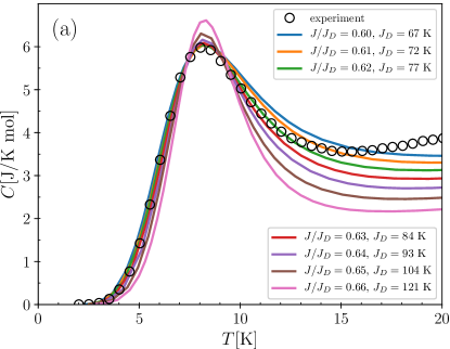
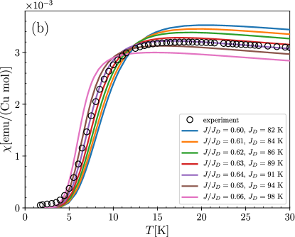
In Fig. 17(a) it is safe to say that the best account of the low-$T$ peak in $C(T)$ is given by $J/J_{D}=0.62$, with $J_{D}=77$ K. Somewhat surprisingly, it is not necessary to exploit to its limits our abilities to resolve a very narrow peak in $C(T)$, as would be the case at higher coupling ratios. Because $J_{D}$ is constrained by many other aspects of the experimental data for SrCu₂(BO₃)₂, its strong dependence on $J/J_{D}$ serves as a strict constraint on the coupling ratio. Turning to Fig. 17(b), the best account of $\chi(T)$ is given by $J/J_{D}=0.64$, with $J_{D}=91$ K. Here it is safe to say that the fits in both panels of Fig. 17 are difficult to reconcile, certainly at the experimentally determined value of $g_{c}$, and as a result we can conclude that we have found the limits of the Shastry-Sutherland model when applied to the SrCu₂(BO₃)₂ problem. It is known that the appropriate spin Hamiltonian for this material contains additional terms, most notably an interlayer coupling, whose magnitude has been estimated at 9% of $J_{D}$ Miyahara and Ueda (2003), and Dzyaloshinskii-Moriya interactions both within and normal to the plane of the system, whose magnitudes have been estimated Nojiri et al. (2003) for both components at 3% of $J_{D}$. Because it is not the purpose of our present analysis to address these details, for further comparison in the present context we restrict our attention to establishing the optimal Shastry-Sutherland fit for SrCu₂(BO₃)₂, to which end we adopt the compromise coupling ratio $J/J_{D}=0.63$ and find that the corresponding optimal $J_{D}$ is 87 K.

Figure 18: Comparison of experimental measurements of the magnetic specific heat, taken from Ref. Kageyama et al. (2000b) and with a phonon contribution $0.5\,T^{3}\,{\rm mJ}/({\rm mol}\,{\rm K}^{4})$ subtracted, to numerical calculations performed by ED, TPQ, and $D=18$ iPEPS for $J/J_{D}=0.63$ with $J_{D}=87$ K.

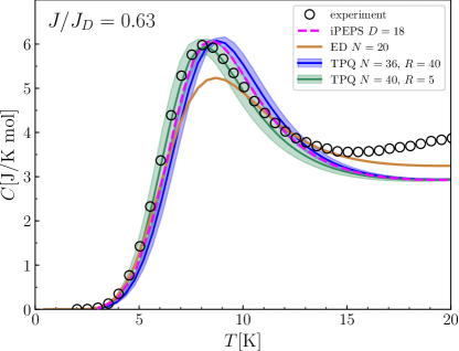
In Fig. 18 we show a quantitative comparison between the results of Sec. IV, specifically Fig. 9, and the $C(T)$ data of Ref. Kageyama et al. (2000b). We observe that our best TPQ results ($N=40$) and our iPEPS results separately provide quantitatively excellent fits to the measured data. Our conclusion that such a fit is optimized with the coupling ratio $J/J_{D}=0.63$ is in accordance with the suggestion, made on the basis of small-system ED calculations, of Ref. Miyahara and Ueda (2000). Further, our determination of the coupling constant, $J_{D}=87$ K, from the precisely known position, $T^{C}_{\max}$ [Fig. 17(a)], of the $C(T)$ peak, is also close to the parameters deduced 20 years ago. As noted above, while these constants may also be constrained from high-$T$ and magnetization information, our results demonstrate finally that they are consistent with the hitherto mysterious low-$T$ behavior.

Figure 19: (a) Comparison of experimental measurements of the magnetic susceptibility, taken from Ref. Kageyama et al. (1999b), to numerical calculations performed by ED, TPQ, and $D=18$ iPEPS for $J/J_{D}=0.63$. We use $g=2.28$ and $J_{D}=87$ K. (b) Detail of the comparison at low temperatures.

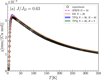
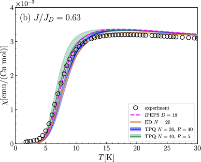
We stress that, despite reaching the previously unattainable goal of reproducing the true shape of the low-$T$ peak in $C(T)$, indeed for coupling ratios even higher than $J/J_{D}=0.63$, we do not find that a sharper peak is required to explain experiment (our results at $J/J_{D}\geq 0.64$ tend to exceed the experimental peak height). Thus we deduce that, to the extent that the Shastry-Sutherland model offers an acceptable account of the physics of SrCu₂(BO₃)₂ (i.e. to the extent that 3D and Dzyaloshinskii-Moriya interactions may be neglected), the coupling ratio is $J/J_{D}=0.63\pm 0.01$. We have based this estimate on reproducing the shape of the low-$T$ peak in $C(T)$; if we consider the dip region at higher temperatures, Fig. 18 shows a significant discrepancy between experiment and our best peak fits, but because the question of subtracting the phonon contribution becomes more important here it is difficult to ascribe the same quantitative reliability to our fits.

In Fig. 19, we perform the same exercise by showing a quantitative comparison between our results (Sec. IV) and the data of Ref. Kageyama et al. (1999b) for the magnetic susceptibility of SrCu₂(BO₃)₂. Again we use the value $J_{D}=87$ K along with the $g$-factor $g_{c}=2.28$ noted above. We show the entire temperature range in Fig. 19(a), which emphasizes the very abrupt peak and the reliability of our model at all high temperatures. In Fig. 19(b) we focus on the low-temperature regime, where again the half-height, $T_{1/2}^{\chi}$, admits only a rather narrow range of coupling ratios. Thus our improved computational methods confirm both the extent to which SrCu₂(BO₃)₂ can be approximated by a pure Shastry-Sutherland model and the efficacy of the parameter estimates made two decades ago on the basis of significantly inferior numerical technology.

VI Summary and Perspectives

We have introduced two advanced numerical techniques, the methods of typical pure quantum (TPQ) states and infinite projected entangled-pair states (iPEPS), for computing the thermodynamic properties of quantum magnets. Both approaches are unaffected by frustration and we apply them to compute the magnetic specific heat and susceptibility of the Shastry-Sutherland model in its dimer-product phase near the first-order quantum phase transition (QPT) to a plaquette phase. This challenging region of coupling ratios has remained entirely impervious to meaningful analysis by any previous numerical techniques, and now we are able to reveal why. The specific heat develops an increasingly narrow low-temperature peak, which is separated from the broad hump due to local processes by an emerging dip. This peak is caused by a proliferation of low-lying energy levels whose origin lies in scattering states of multiple two-triplon bound states, and its anomalously low energy scale moves ever lower (albeit not to zero) as the QPT is approached. The analogous feature in the magnetic susceptibility is an increasingly rapid rise at an ever-lower temperature, followed by an abrupt maximum. This physics is a consequence of both high frustration and the proximity to a QPT, and its manifestations have been discussed previously in highly frustrated 1D systems, but now we have captured its realization in 2D.

Our methods and benchmarks offer very wide scope for immediate application. The list of open problems in frustrated quantum magnetism is long, and we await with interest definitive results, meaning for extended or spatially infinite systems, for the thermodynamic response of the triangular, kagome, and $J_{1}$-$J_{2}$ square lattices. The ability to fingerprint the energy spectrum at the level of thermodynamic properties will provide a new dimension of physical understanding, and in some cases may even yield new insight into the ground state. Away from the classic problems of geometrical frustration in Heisenberg models, there is a pressing need for thermodynamic information to characterize many other types of frustrated system, including spin-ice materials, candidate Kitaev materials, coupled anisotropic (Ising and XY) chain and planar materials, candidate chiral spin liquids, materials with Dzyaloshinskii-Moriya interactions, topological magnets, and certain skyrmion systems.

Technically, neither of our methods presents any barrier to the application of a magnetic field, which could be used to control the relative singlet and triplet gaps and create qualitative changes in the thermodynamic response in many of the above types of system. For the SrCu₂(BO₃)₂ problem, the next step enabled by the capabilities developed here is clearly to follow the evolution of the system to and through the pressure-induced QPT into the plaquette phase Zayed et al. (2017); Guo et al. . This process presents a clear need for the investigation of thermodynamic properties, even if the physics of the material beyond the dimer-product phase is critically dependent on additional Hamiltonian terms beyond the Shastry-Sutherland model.