Abstract

We study rectangular timelike Wilson loops at long distances in the exact renormalization group flow in the context of the holographic duality. We consider the 5d holographic model with an exponential dilaton potential constructed in [arXiv:1803.06764]. To probe the RG flow backgrounds at zero and finite temperatures we calculate the minimal surfaces of the corresponding string worldsheets. We show that a holographic RG flow at $T=0$,that mimics QCD behaviour of the running coupling, has a confining phase at long distances, while the RG flow with an AdS UV fixed point is non-confining.

1 Introduction

In the recent years the holographic correspondence [1]-[3] has been shown to be a very useful tool to get theoretical insight into systems in the strongly coupling regime [4, 5]. In the holographic prescription renormalization group flows of field theories are realized as gravitational domain-wall solutions interpolating between boundaries [6]-[9]. These boundaries of the solutions are supposed to be related to fixed points of a dual field theory and should have particular properties. The radial position in the bulk geometry corresponds to the energy scale, while the dilaton is related to the running coupling[10]. Various non-perturbative phenomena that are inaccessible in the dual field theory can be captured by the holographic RG flow [11, 12]. There is a class of useful bottom-up holographic models [14]-[16], that are of interest because they can be studied analytically resembling features of the real QCD, in particular the running coupling [17, 18].

In [18] exact holographic RG flows for a model with the dilaton potential which represents a sum of two exponential functions were constructed. From one side the choice of the potential is motivated by applications to studies of late-time behaviour of the quark-gluon plasma [19]. Particularly, a single exponential potential, used in [19], corresponds to the IR limit of the improved holographic QCD potentials [11, 12]. The case of the dilaton potential with two exponential terms was also considered in [13].

Secondly, the motivation for the model comes from a possible supergravity embedding where exponential terms can be related with the contribution of $0$-th forms [20]. In the context of the holographic RG flow the gravity model with simple exponential was discussed in [21]. The model in [18] appears to be solvable and can be reduced to $A_{1}\times A_{1}$ Toda chain. It was shown that the behaviour of the running coupling $\lambda$ built on the analytic solutions can mimic that one we see in QCD. Namely, one can observe an infinite value of $\lambda$ in the IR region and an asymptotic freedom in the UV limit. Moreover, for the finite temperature case the dependence of the free energy on the temperature signalized the Hawking-Page phase transition. Hereby it is of interest to perform a check if the confinement takes place for the backgrounds found in [18].

The Wilson loop represents one of criteria for studies of the IR region and manifests an area law behaviour in the case of the confinement. Via the holographic approach Wilson loops has been widely used to consider in different settings. Following [22]-[25] the holographic Wilson loops can be obtained minimising the world-sheet action of a string living in the gravity background with endpoints on the boundary contour. Wilson loops in various holographic RG flows were studied in [26]-[31]. In [26]-[29] Wilson loops were discussed in holographic renormalization group flows in the framework of 5d gauged supergravities. In [17, 30] holographic Wilson loops with different orientations were studied in the holographic RG flows constructed for the spatially anisotropic model with quadratic dilaton and Maxwell fields [17]. It was shown in [30] that the holographic model has a confinement phase and the phase diagram includes both the Wilson transition and Hawking-Page phase transition lines, which can have a common point. It is interesting to note that the dilaton potential from [17], which is restored for their solutions, has the same shape as the dilaton potential considered in [18]. In [31] it was proposed a general method of Wilsonian renormalization to a string stretched in the holographic RG flow background.

In this work we shall consider holographic time-like rectangular Wilson loops for the backgrounds found in [18] that can be associated with the holographic RG flows. We consider both the case of zero and finite temperature. Using the method developed in [18, 32], based on introducing a so-called effective potential $V_{eff}$, we estimate the behaviour of holographic Wilson loops at long distances. It is supposed that the confinement phase takes place when $V_{eff}$ has a critical point. We show that $V_{eff}$ corresponding to the holographic RG flow at $T=0$, which running coupling mimics the QCD behaviour, can indeed have a critical point under certain constraints, i.e. this background has a confinement phase in the IR region.

The structure of the paper is organized as follows. In Sec. 2 we give an overview of the model and the corresponding generic solutions. We also briefly discuss the asymptotic behavior of the solutions at $T=0$. In Sec. 3 we explore holographic Wilson loops at zero temperature. In Sec. 4 we describe the black hole solution in short and estimate the behaviour of the Wilson loops in the holographic RG flows at finite temperature. In Appendix A we present the useful relations for extremal points of $V_{eff}$ in the confining background at $T=0$.

2 The setup

2.1 The holographic model

Our starting point is a 5d holographic model [18] governed by an action of the form

$$\mathcal{S}=\frac{1}{16\pi G_{5}}\int d^{5}x\sqrt{|g|}\left(R-\frac{4}{3}\left(\partial\phi\right)^{2}-C_{1}e^{2k_{1}\phi}-C_{2}e^{2k_{2}\phi}\right)+G.H.,$$ (2.1)

where $C_{i}$, $k_{i}$ with $i=1,2$ are constants. We choose the constants $C_{1}$ and $C_{2}$ as follows

$$C_{1}<0,\quad C_{2}>0.$$ (2.2)

Putting the constraint on the dilatonic constants as $k_{1}=k$, $k_{2}=\frac{16}{9k}$, with $0<k<4/3$, one can reduce the model (2.1) to the $A_{1}\times A_{1}$ Toda chain [18]. The general form of the solutions for EOM following from (2.1) is given by the metric

$$ds^{2}=F^{\frac{8}{9k^{2}-16}}_{1}F^{\frac{9k^{2}}{2(16-9k^{2})}}_{2}\left(-e^{2\alpha^{1}u}dt^{2}+e^{-\frac{2\alpha^{1}}{3}u}d\vec{x}^{\leavevmode\nobreak\ 2}\right)+F^{\frac{32}{9k^{2}-16}}_{1}F^{\frac{18k^{2}}{16-9k^{2}}}_{2}du^{2},$$ (2.3)

where $\vec{x}=(x_{1},x_{2},x_{3})$ and the corresponding dilaton

$$\phi=-\frac{9k}{9k^{2}-16}\log{F_{1}}+\frac{9k}{9k^{2}-16}\log{F_{2}}.$$ (2.4)

The functions $F_{1}$ and $F_{2}$ in (2.3)-(2.4) are given by

$$F_{1} = \sqrt{\left|\frac{C_{1}}{2E_{1}}\right|}\sinh(\mu_{1}\,|u-u_{01}|),\,\mu_{1}=\sqrt{\left|\frac{3E_{1}}{2}\left(k^{2}-\frac{16}{9}\right)\right|},$$ (2.5)

$$F_{2} = \sqrt{\left|\frac{C_{2}}{2E_{2}}\right|}\sinh(\mu_{2}\,|u-u_{02}|),\,\mu_{2}=\sqrt{\left|\frac{3E_{2}}{2}\left(\left(\frac{16}{9}\right)^{2}\frac{1}{k^{2}}-\frac{16}{9}\right)\right|},$$ (2.6)

where $0<k<4/3$, $C_{1}$ and $C_{2}$ are given by (2.2).

We note that the constants of integration are related by the zero energy constraint

$$E_{1}+E_{2}+\frac{2(\alpha^{1})^{2}}{3}=0,$$ (2.7)

with $E_{1}<0$, $E_{2}>0$.

So the general case gives two classes of the solutions, namely, the solutions that possess the Poincaré invariance with the parameter $\alpha^{1}=0$ and those solutions with $\alpha^{1}\neq 0$, i .e. that doesn’t have the Poincaré symmetry. From the solutions with the broken Poincaré symmetry we can construct regular black holes, that the parameter $\alpha^{1}$ can be related to the Hawking temperature.

Moreover, we also have constants of integration $u_{01}$, $u_{02}$, that split our solutions into three charts : a)$u<u_{02}$; b)$u_{02}<u<u_{01}$; c)$u>u_{01}$; we also aim to consider the degenerate case with $u_{01}=u_{02}=u_{0}$. This special case leads to the vacua with the AdS boundary in the UV limit.

We note that all branches of solutions with $\alpha^{1}=0$ are the Poincaré invariant domain walls, but not all of them can be interpreted as holographic RG flows. This can be seen from the behaviour of a scale factor of a certain background. Here it’s convenient to come to the domain wall coordinates, thus the generic metric takes the form

$$ds^{2}=e^{2\mathcal{A}(w)}\left(-dt^{2}+d\vec{x}^{2}\right)+dw^{2}.$$ (2.8)

We note that the change of the coordinates is given by

$$dw = F^{\frac{16}{9k^{2}-16}}_{1}F^{\frac{9k^{2}}{16-9k^{2}}}_{2}du,$$ (2.9)

so the scale factor is

$${\cal A} = \frac{4}{9k^{2}-16}\,\log F_{1}+\frac{9k^{2}}{4(16-9k^{2})}\,\log F_{2}.$$ (2.10)

The quantity $e^{\mathcal{A}}$ is supposed to be associated with the energy scale of the dual theory, while $e^{\phi}$ is related to running coupling. So it supposed that $e^{\mathcal{A}}$ should be monotonic.

a   b   c  

Figure 1: The behaviour of $e^{\mathcal{A}}$ as a function on $\phi$ for solutions defined: a) on the region $(-\infty,u_{02})$ with $u_{02}=-1$; b) $(u_{02},u_{01})$ with $u_{01}=0,u_{02}=-1$; c) $(u_{01},+\infty)$ with $u_{01}=0$ by solid curves, the solution with $u_{01}=u_{02}=0$ by the dashed curve for $E_{1}=-E_{2}=0.01$. For all plots we fix the potential $k=1$, $C_{1}=-C_{2}=1$, varying values of $E_{1}=-E_{2}$ (labeled as $E$ on the plot), except the solution c) defined on $(u_{0};+\infty)$.

From figure 1 a) we see that $e^{\mathcal{A}}$ plotted for the left solution is non-monotonic, and therefore it cannot be interpreted as a holographic RG flow. In what follows we skip the discussion of this solution and its application. At the same time, one can observe from figs. 1 b) and c) that $e^{\mathcal{A}}$ behaves monotonically both for the middle and the right solutions. The case with an AdS boundary has also the monotonic scale factor as it can be seen from Fig. 1 c).

2.2 Boundaries of the holographic RG flows at zero temperature

Here we give a review of the asymptotics of the middle and right solutions with $\alpha^{1}=0$. As we said before, these are Poincaré invariant domain wall solutions, that can be considered as holographic renormalization group flows at zero temperature.

The middle solution is defined on the region $(u_{02},u_{01})$. The metric and the dilaton near the boundary with $u\to u_{02}+\epsilon$ are

$$ds^{2} \sim (\mu_{2}(u-u_{02}))^{\frac{9k^{2}}{2(16-9k^{2})}}(-dt^{2}+d\vec{x}^{2})+(\mu_{2}(u-u_{02}))^{\frac{18k^{2}}{16-9k^{2}}}du^{2},$$ (2.11)

$$\lim_{u\to u_{02}-\epsilon}\phi \sim -\frac{9k}{16-9k^{2}}\log\left(\sqrt{\frac{C_{2}}{C_{1}}}\frac{\mu_{2}\,\epsilon}{\sinh(\mu_{1}\,(u_{01}-u_{02}))}\right)\to+\infty.$$ (2.12)

Taking into account the plot  1 b) we see that with the dilaton going to $+\infty$ the energy scale $e^{\mathcal{A}}$ tends to $0$, so one can associate this boundary with the IR region. We note that this boundary is a conformally flat spacetime, the sign of the scalar curvature depends on the choice of the shape of the potential, i.e. the value of the dilaton coupling $k$ [18].
Another boundary of the middle solution is this one near $u_{01}$. Here the metric reads

$$ds^{2} \sim (\mu_{1}(u-u_{01}))^{\frac{8}{9k^{2}-16}}(-dt^{2}+d\vec{x}^{2})+(\mu_{1}(u-u_{01}))^{\frac{32}{9k^{2}-16}}du^{2},$$ (2.13)

and the dilaton is

$$\phi_{u\to u_{01}+\epsilon} \sim -\frac{9k}{16-9k^{2}}\log\left(\sqrt{\left|\frac{C_{2}}{C_{1}}\right|}\frac{\sinh(\mu_{2}\,(u_{01}-u_{02}))}{\mu_{1}\,\epsilon}\right)\to-\infty.$$ (2.14)

This boundary is also conformally flat spacetime spacetime with the sign of the scalar curvature depending on the value $k$. Looking on the plot 1 b) we see that the energy scale corresponding to the middle solution goes to $+\infty$ as the dilaton tends to $-\infty$. Thus, one can say that the boundary near $u_{01}$ is the UV limit and we see the asymptotic freedom near it.

Now we turn to the right solution that is defined for the region $(u_{01},+\infty)$. The first boundary of the right solution is near $u_{01}$ point and the asymptotics of the metric and the dilaton coincide with those for the middle solution (2.13)-(2.14). With respect to Fig. 1 c) we can also say that this boundary corresponds to the UV region.
For the other boundary with $u\to+\infty$ the metric reads

$$ds^{2} \sim e^{-\frac{2\mu_{1}u}{4+3k}}\left(-dt^{2}+d\vec{x}^{2}\right)+e^{-\frac{8\mu_{1}u}{4+3k}}du^{2},$$ (2.15)

and the dilaton

$$\phi_{u\to+\infty} \sim -\frac{9k}{16-9k^{2}}\Big{[}(\mu_{2}-\mu_{1})\,u+\frac{1}{2}\log|\frac{C_{2}}{C_{1}}|\Big{]}\to-\infty.$$ (2.16)

From Fig. 1c) we see that the scale factor goes to $-\infty$ as the dilaton tends to $-\infty$ and we observe the IR free theory. We remind that the dilaton tends to $-\infty$ near the other boundary is well so the dilaton is bouncing. We note that the boundary of the right solution with $u\to+\infty$ is also a conformally flat spacetime with the positive curvature.

The special case of the solution defined on the region $(u_{0},+\infty)$ with the points $u_{01}=u_{02}=u_{0}$ is of particular interest.

The metric near the boundary with $u\to u_{0}+\epsilon$ tends to be a 5d AdS spacetime

$$\begin{split}ds^{2}&\sim\left(\frac{4}{3k}\right)^{\frac{9k^{2}-16}{2(16-9k^{2})}}[\mu_{1}(u-u_{0})]^{-\frac{1}{2}}(-dt^{2}+d\vec{x}^{2})+\left(\frac{4}{3k}\right)^{\frac{18k^{2}}{16-9k^{2}}}[\mu_{1}(u-u_{0})]^{-2}du^{2}.\end{split}$$ (2.17)

In (2.17) one can easily recognize the 5d AdS metric supported by the constant dilaton

$$\phi_{u\to u_{0}}\sim\frac{9k}{(16-9k^{2})}\log\frac{3k}{4}+\frac{9k}{2(16-9k^{2})}\log\Big{|}\frac{C_{1}}{C_{2}}\Big{|},$$ (2.18)

which coincides with the minimum of the potential.
Introducing a new conformal ”radial” coordinate as $z=4(u-u_{0})^{1/4}$ one represents the solution in the Poincare patch

$$ds^{2}\sim\frac{1}{z^{2}}(-dt^{2}+dx^{2}_{1}+dx^{2}_{2}+dx^{2}_{3}+dz^{2}),$$ (2.19)

where $z\to 0$ as $u\to u_{0}$. The energy scale $e^{\mathcal{A}}$ takes big values with constant dilaton, see fig. 1 c), so this boundary is related to the UV fixed point.

The asymptotics of the metric and the dilaton with $u\to+\infty$ coincide with those relations for the ”right” solution and correspond to the IR-region.

To summarize, we have three holographic RG flows at zero temperature, namely:

1. the middle solution defined for $u\in(u_{02},u_{01})$ interpolates between two different hyperscaling violating boundaries that can be associated with the weakly coupled UV fixed point and the IR fixed point at strong coupling;

2. the right solution defined for $u\in(u_{01},+\infty)$ represents an RG flow with UV and IR fixed points corresponding to a free theory. It also has two different hyperscaling violating boundaries;

3. the special case defined for $u\in(u_{02},u_{01})$ with $u_{02}=u_{01}=u_{0}$, when the solution interpolates between AdS-boundary in the UV limit and hyperscaling violating boundary in the IR limit.

We would like to note that the boundary near $u_{01}$ corresponds to the UV region both holographic RG flows defined on $(u_{01},u_{02})$ and $(u_{0},+\infty)$.

3 Wilson loops in holographic RG flow at zero T

The expectation value of the rectangular temporal Wilson loop of size $T\times\ell$ is related with the potential between a quark and an antiquark on a distance $\ell$ as

$$\Braket{W}\sim e^{-V_{q\bar{q}}(\ell)T}.$$ (3.1)

At the same time the holographic Wilson loop can be defined through the Nambu-Goto action $\mathcal{S}_{NG}$ of a string in a considered background [22, 23]

$$\Braket{W(\mathcal{C})}\sim e^{-\mathcal{S}_{NG}}.$$ (3.2)

So one can estimate the potential of the quark-antiquark interaction as

$$V_{q\bar{q}}=\frac{1}{T}\mathcal{S}_{NG}.$$ (3.3)

The Nambu-Goto action is defined as

$$\mathcal{S}_{NG}=-\frac{1}{2\pi\alpha^{\prime}}\int d^{2}\sigma\sqrt{-\det{h}},$$ (3.4)

where we use the string frame for the induced metric

$$h_{\alpha\beta}=e^{\frac{4}{3}\phi}G_{\mu\nu}\partial_{\alpha}X^{\mu}\partial_{\beta}X^{\nu},$$ (3.5)

with the world-sheet coordinated $\sigma^{\alpha}$, $\alpha=0,1$, and the embedding functions $X^{\mu}=X^{\mu}(\sigma^{\alpha})$.

In this section we discuss the Nambu-Goto action for the general solution (2.3) with $\alpha^{1}=0$ in the domain wall coordinates (2.8). This corresponds to consideration of Wilson loops in the holographic RG flows. For the string configuration we choose the following gauge [22]

$$\sigma^{0}=t,\quad\sigma^{1}=x_{1},\quad w=w(x_{1}),$$ (3.6)

supposing that $w(0)=w(\ell)=0$, $w\left(\frac{\ell}{2}\right)=w_{*}$.

Then the induced metric has the following form

$$ds^{2}=e^{\frac{4}{3}\phi}\left(-e^{2\mathcal{A}}dt^{2}+(e^{2\mathcal{A}}+w^{\prime 2})dx^{2}_{1}\right).$$ (3.7)

The Nambu-Goto action in the string frame is related to introducing the dilaton multiplier in the following way

$$\begin{split}\mathcal{S}_{NG}&=-\frac{1}{2\pi\alpha^{\prime}}\int dx_{1}dte^{\frac{4\phi}{3}}\sqrt{e^{2\mathcal{A}}(e^{2\mathcal{A}}+w^{\prime 2})}.\end{split}$$ (3.8)

The equation for the turning point following from (3.8) reads

$$x^{\prime}_{1}=\frac{c}{e^{\mathcal{A}}\sqrt{e^{4\mathcal{A}+\frac{8}{3}\phi}-c^{2}}},$$ (3.9)

where $x^{\prime}_{1}=\frac{dx_{1}}{dw}$ and $c$ is a constant, i.e. $c=e^{2\mathcal{A}(w_{*})}$. Now it’s convenient to come to the original $u$-coordinate using

$$\begin{split}x^{\prime}_{1}&=\frac{dx_{1}}{dw}=\frac{dx_{1}}{du}\frac{du}{dw}=e^{-4\mathcal{A}}\dot{x}_{1},\end{split}$$ (3.10)

where we take into account (2.9)-(2.10) and denote $\dot{x}_{1}=\frac{dx_{1}}{du}$.

From (3.9)-(3.10) one can find the distance between quarks as

$$\begin{split}\frac{\ell}{2}&=\int du\frac{ce^{3\mathcal{A}}}{\sqrt{e^{4\mathcal{A}+\frac{8}{3}\phi}-c^{2}}}\end{split}$$ (3.11)

and for the Nambu-Goto action we have the following relation

$$\begin{split}\frac{\mathcal{S}_{NG}}{2}&=\frac{T}{2\pi\alpha^{\prime}}\int{du}\frac{e^{7\mathcal{A}+\frac{8\phi}{3}}}{\sqrt{e^{4\mathcal{A}+\frac{8\phi}{3}}-c^{2}}}.\end{split}$$ (3.12)

Let us define the so-called effective potential with $u^{\prime}=0$ [30, 32] as

$$V_{eff}=e^{2\mathcal{A}+\frac{4}{3}\phi}=F_{1}^{\frac{4(2-3k)}{9k^{2}-16}}F_{2}^{\frac{3k(3k-8)}{2(16-9k^{2})}}.$$ (3.13)

a   b
 
c   d   e 

Figure 2: $V_{eff}$ as a function of $u$ for the holographic RG flows: a),b) defined on $(u_{02};u_{01})$ with $u_{02}=-1$, $u_{01}=0$ for small and big $k$, correspondingly; c),d) defined on $(u_{01};+\infty)$ with $u_{01}=0$ for small and big $k$, correspondingly; e) with coinciding points $u_{01}=u_{02}=0$. For all $E_{1}=E_{2}=-1$, $C_{1}=-C_{2}=-1$.

In terms of $V_{eff}$ the quark-antiquark distance can be presented as

$$\frac{\ell}{2}=\int du\,e^{-2\phi}\frac{V_{eff}(u)\sqrt{V_{eff}(u)}}{\sqrt{\frac{V^{2}_{eff}(u)}{V^{2}_{eff}(u_{*})}-1}}$$ (3.14)

and the string action is given by

$$\frac{\mathcal{S}_{NG}}{2} = \frac{T}{2\pi\alpha^{\prime}}\int{du}\frac{e^{-2\phi}V^{3}_{eff}(u)\sqrt{V_{eff}(u)}}{\sqrt{V^{2}_{eff}(u)-V^{2}_{eff}(u_{*})}}.$$ (3.15)

One can see from (3.14)-(3.15) that we have to require the function $V_{eff}$ to be decreasing on the region $(u_{01},u_{*})$. It can be also seen from (3.14)-(3.15) that to observe a confinement in the IR region, that implies $\ell\to+\infty$ with $\mathcal{S}_{NG}\to+\infty$, $V_{eff}$ needs have a local minimum. Let’s suppose that

$$V^{\prime}_{eff}(u)|_{u=u_{min}}=0,\quad V^{{}^{\prime\prime}}_{eff}(u_{min})>0.$$ (3.16)

Then, expanding in the Taylor series at the point $u_{min}$, with $u_{min}=u_{*}$ one has

$$\frac{V^{2}_{eff}(u)}{V^{2}_{eff}(u_{min})}=1+\frac{V^{\prime\prime}(u_{min})}{V_{eff}(u_{min})}(u-u_{min})^{2}+\mathcal{O}(u-u_{min})^{2}.$$ (3.17)

We note that the constraint $V^{\prime}_{eff}=0$ leads to the equation

$$2(2-3k)\frac{\cosh(\mu_{1}(u-u_{01}))}{\sinh(\mu_{1}(u-u_{01}))}-(3k-8)\frac{\cosh(\mu_{2}(u-u_{02}))}{\sinh(\mu_{2}(u-u_{02}))}=0,$$ (3.18)

which we need to study separately for each holographic RG flow.

Remembering that the holographic RG flow is splitted into 3 branches one has to analyze the behaviour of (3.13)-(3.18) for each case of the holographic RG flows.

1. For holographic RG flow defined on $(u_{02};u_{01})$ (the middle solution ) the worldsheet boundary is attached at $u_{01}$. The distance between quarks reads

   $$\frac{\ell}{2}=\int^{u_{01}}_{u_{*}}du\,\frac{c\,e^{-2\phi}V^{3/2}_{eff}}{\sqrt{V^{2}_{eff}-V^{2}_{eff}(u_{*})}}.$$ (3.19)

   The string action is divergent at the UV boundary, the renormalized Nambu-Goto action takes the form

   $$\mathcal{S}^{\,\,\,ren}_{NG}=\frac{T}{\pi\alpha^{\prime}}\int^{u_{01}}_{u_{*}}du\,\left(\frac{e^{-2\phi}V^{7/2}_{eff}}{\sqrt{V^{2}_{eff}-V^{2}_{eff}(u_{*})}}-e^{-2\phi}V^{5/2}_{eff}\right)+\frac{T}{\pi\alpha^{\prime}}\int^{u_{01}-u_{(\Lambda)}}_{u_{*}}du\,e^{-2\phi}V^{5/2}_{eff},$$

   where $u_{(\Lambda)}<0$ and the singular term at the boundary $u_{01}$ reads

   $$\lim_{u\to u_{01}-\epsilon}e^{-2\phi}V^{5/2}_{eff}\sim(\sqrt{\left|\frac{C_{2}}{2E_{2}}\right|}\sinh(\mu_{2}(u_{01}-u_{02})))^{\frac{3k(15k-16)}{4(16-9k^{2})}}(\sqrt{\left|\frac{C_{1}}{2E_{1}}\right|}(\mu_{1}(u-u_{01}))^{\frac{4(5-3k)}{9k^{2}-16}}.$$

   

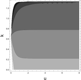
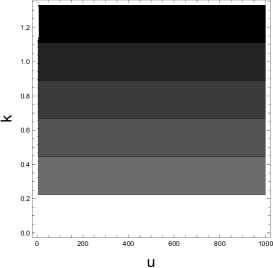
   a  b  c

   Figure 3: The solutions to the equation (3.18) defined on different regions: a) $(u_{02},u_{01})$ with $u_{02}=-1$, $u_{01}=0$; b) $(u_{01},+\infty)$, $u_{01}=0$; c) $u_{01}=u_{02}=0$.

   By virtue of (1) one can represent (1) in the following form

   $$\mathcal{S}^{ren}_{NG}=\frac{T}{\pi\alpha^{\prime}}\int^{u_{01}}_{u_{*}}du\,\Bigl{(}\frac{e^{-2\phi}V^{7/2}_{eff}}{\sqrt{V^{2}_{eff}-V^{2}_{eff}(u_{*})}}-e^{-2\phi}V^{5/2}_{eff}\Bigr{)}$$

   $$- \frac{T}{\pi\alpha^{\prime}}\frac{2\sqrt{3}}{(2-3k)^{2}\sqrt{|C_{1}|}}(\sqrt{\frac{|C_{2}|}{2|E_{2}|}}\sinh(\mu_{2}(u_{01}-u_{02})))^{\frac{3k(15k-16)}{4(16-9k^{2})}}(\sqrt{\frac{|C_{1}|}{2|E_{1}|}}(\mu_{1}|u_{*}-u_{01}|)^{\frac{(3k-2)^{2}}{9k^{2}-16}}.$$

   We note that in the UV limit $V_{eff}|_{u\to u_{01}-\epsilon}$ tends $+\infty$ for $k<2/3$ and goes to $0$ for $k>2/3$, while in the IR limit ($u\to u_{02}+\epsilon$) it always tends to $+\infty$ for all $k$. From figure 2 a) we see that the function $V_{eff}$ has one minimum, for small values $k$ ($k<\frac{2}{3}$). At the same time from figure 2 b) one can observe that for the same RG flow with $k>\frac{2}{3}$ $V_{eff}$ doesn’t have any extremal point, so $V^{\prime}_{eff}\neq 0$. Indeed from figure 3 a) one can see that equation (3.18), corresponding to the RG flow on the region $(u_{02};u_{01})$, has a solution for $k<2/3$, while for $k>\frac{2}{3}$ it does not have solutions. Hereby,

   • for $k<2/3$ taking into account $V^{\prime}_{eff}(u_{min})=0$ and plugging (3.17) in (3.14)-(3.15) the quark-antiquark distance reads

     $$\frac{\ell}{2}=\int^{u_{01}}_{u_{min}}\frac{e^{-2\phi}V^{2}_{eff}(u_{min})du}{\sqrt{V^{\prime\prime}_{eff}(u_{min})}(u_{min}-u)}\sim\frac{e^{-2\phi(u_{min})}V^{2}_{eff}(u_{min})}{\sqrt{V^{\prime\prime}_{eff}(u_{min})}}\log(u_{min}-u),$$ (3.23)

     and the Nambu-Goto action is given by

     $$\mathcal{S}_{NG}=\int^{u_{(\Lambda)}}_{u_{min}}\frac{e^{-2\phi}V^{3}_{eff}(u_{min})du}{\sqrt{V^{\prime\prime}_{eff}(u_{min})}(u_{min}-u)}\sim\frac{e^{-2\phi(u_{min})}V^{3}_{eff}(u_{min})}{\sqrt{V^{\prime\prime}_{eff}(u_{min})}}\log(u_{min}-u),$$

     so $\ell\to+\infty$ with $\mathcal{S}_{NG}\to+\infty$ as $u\to u_{min}$. From (3.23)-(• ‣ 1) we have

     $$\mathcal{S}_{NG}\sim\sigma\ell,$$ (3.25)

     with $\sigma=V_{eff}(u_{min})$. So at large distances one has a linear growth of the heavy quark potential;

   • if $k>2/3$ we have $V^{\prime}_{eff}\neq 0$ according to figure 2 b) and we can not reach the regime of large $\ell$.

   Therefore, one has a confinement phase for $k<\frac{2}{3}$ and deconfinement phase for $k>\frac{2}{3}$. We note that in [18] it was shown that the holographic RG flow defined on the region $(u_{02};u_{01})$ reproduces the QCD behaviour of the running coupling.

2. For the holographic RG flow defined on $(u_{01};+\infty)$ (the right solution) the worldsheet boundary is attached at $u_{01}$ again. The distance between quarks reads

   $$\frac{\ell}{2}=\int^{u_{*}}_{u_{01}}du\,\frac{c\,e^{-2\phi}V^{3/2}_{eff}}{\sqrt{V^{2}_{eff}-V^{2}_{eff}(u_{*})}}.$$ (3.26)

   The Nambu-Goto action is divergent near $u_{01}$ boundary, after the renormalization one has

   $$\mathcal{S}^{\,\,ren}_{NG}=\frac{T}{\pi\alpha^{\prime}}\int^{u_{*}}_{u_{01}}du\,\left(\frac{e^{-2\phi}V^{7/2}_{eff}}{\sqrt{V^{2}_{eff}-V^{2}_{eff}(u_{*})}}-e^{-2\phi}V^{5/2}_{eff}\right)$$

   $$+\frac{T}{\pi\alpha^{\prime}}\frac{2\sqrt{3}}{(2-3k)^{2}\sqrt{|C_{1}|}}(\sqrt{\frac{C_{2}}{2E_{2}}}\sinh(\mu_{2}(u_{01}-u_{02})))^{\frac{3k(15k-16)}{4(16-9k^{2})}}(\sqrt{\frac{|C_{1}|}{2|E_{1}|}}(\mu_{1}|u_{*}-u_{01}|)^{\frac{(3k-2)^{2}}{9k^{2}-16}}.$$

   $V_{eff}|_{u\to u_{01}+\epsilon}$ tends to $+\infty$ for $k<2/3$ and to $0$ for $k>2/3$ near the $UV$ fixed point. In the IR limit $V_{eff}$ goes to $0$ for all k. In figure 2 c) we observe that $V_{eff}$ doesn’t have any extremal points with $k<\frac{2}{3}$ , i.e. $V^{\prime}_{eff}\neq 0$. For $k>\frac{2}{3}$ figure 2 d) shows that $V_{eff}$ has a maximum, so $V^{\prime}_{eff}=0$ and $V^{\prime\prime}_{eff}<0$. In figure  3 b) we present the solution to eq.(3.18) on the region $(u_{01},+\infty)$. One can see that there is no solutions for $k<2/3$, while for $k>2/3$ there is a solution, corresponding to maximum of $V_{eff}$. So, one have the background is non-confining for all values of $0<k<4/3$. This is in agreement with [18],where we have seen that the RG flow defined on $(u_{01},+\infty)$ corresponds to the UV and IR free theory.

3. The special case (holographic RG flow with AdS boundary), $u_{01}=u_{02}=u_{0}$. The worldsheet boundary is attached at $u_{0}$. The distance between quarks reads

   $$\frac{\ell}{2}=\int^{u_{*}}_{u_{0}}du\,\frac{c\,e^{-2\phi}V^{3/2}_{eff}}{\sqrt{V^{2}_{eff}-V^{2}_{eff}(u_{*})}}.$$ (3.28)

   The string action is divergent at the UV boundary, the renormalized Nambu-Goto action takes the form

   $$\mathcal{S}^{ren}_{NG}=\frac{T}{\pi\alpha^{\prime}}\int^{u_{*}}_{u_{0}}du\,\left(\frac{e^{-2\phi}V^{7/2}_{eff}}{\sqrt{V^{2}_{eff}-V^{2}_{eff}(u_{*})}}-e^{-2\phi}V^{5/2}_{eff}\right)+\frac{T}{\pi\alpha^{\prime}}\int^{u_{*}}_{u_{0}-u_{(\Lambda)}}du\,e^{-2\phi}V^{5/2}_{eff}.$$

   Since we have

   $$\lim_{u\to u_{0}+\epsilon}e^{-2\phi}V^{5/2}_{eff}\sim|C_{1}|^{\frac{2(5-3k)}{9k^{2}-16}}\left(\frac{4}{3k}\sqrt{C_{2}}\right)^{\frac{3k(15k-16)}{4(16-9k^{2})}}(2E_{1})^{\frac{5}{8}}(\mu_{1}(u-u_{0}))^{-\frac{5}{4}},$$ (3.30)

   so one can represent the remormalized Nambu-Goto action in the following form

   $$\mathcal{S}^{\,\,ren}_{NG} = \frac{T}{\pi\alpha^{\prime}}\int^{u_{*}}_{u_{0}}du\,\left(\frac{e^{-2\phi}V^{7/2}_{eff}}{\sqrt{V^{2}_{eff}-V^{2}_{eff}(u_{*})}}-e^{-2\phi}V^{5/2}_{eff}\right)$$ (3.31)

   $$- \frac{T}{\pi\alpha^{\prime}}|C_{1}|^{\frac{2(5-3k)}{9k^{2}-16}}\left(\frac{4}{3k}\sqrt{C_{2}}\right)^{\frac{3k(15k-16)}{4(16-9k^{2})}}(2E_{1})^{\frac{5}{8}}\frac{4\mu^{-\frac{5}{4}}_{1}}{(u_{*}-u_{0})^{1/4}}.$$

   We note that $V_{eff}$ tends to $+\infty$ as $u\to u_{0}+\epsilon$ and to $0$ with $u\to+\infty$ for all $k$.

   Figure 2  e) shows that $V_{eff}$ corresponding to this RG flow doesn’t have any extremal points defined on $(u_{0};+\infty)$ for all values of $0<k<4/3$. This is confirmed by solutions to eq. (3.18) in figure 3 c). So the holographic RG flow with an AdS UV fixed point is also non-confining. It is consistent with an observation from [18], where it was shown that the running coupling corresponding to this RG flow tends to some finite value in the UV limit and to $0$ in the IR region.

4 Wilson loops in the holographic RG flow at finite temperature.

Now we turn to the discussion of the Wilson loops in the non-zero temperature background found in [18]. It was shown that one can derive the black brane metric from the generic non-Poincaré invariant solutions with non-zero $\alpha^{1}$ (2.3)-(2.7) defined on the region $(u_{01};+\infty)$. It is reached taking $\mu_{1}=\mu_{2}=-\frac{4}{3}\alpha^{1}$, that is possible for the non-Poincaré invariant solutions by virtue of the constraint (2.7). The black hole metric reads

$$ds^{2} = \mathcal{C}\,\mathcal{X}(u)\Big{(}-e^{-2\mu u}dt^{2}+d\vec{x}^{2}\Big{)}+\mathcal{C}^{4}\,\mathcal{X}(u)^{4}e^{-2\mu u}du^{2},$$ (4.1)

where $\mathcal{X}$ and $\mathcal{C}$ are given by

$$\mathcal{X} = (1-e^{-2\mu u})^{-\frac{8}{16-9k^{2}}}(1-e^{-2\mu(u-u_{02})})^{\frac{9k^{2}}{2(16-9k^{2})}},$$ (4.2)

$$\mathcal{C} \equiv 2^{\frac{16}{(16-9k^{2})}}(3\mu)^{\frac{1}{2}}\left|C_{1}\right|^{\frac{8}{2(9k^{2}-16)}}\Big{(}\frac{C_{2}}{k}e^{-2\mu u_{02}}\Big{)}^{\frac{9k^{2}}{4(16-9k^{2})}}(16-9k^{2})^{-\frac{1}{4}}$$ (4.3)

and the corresponding dilaton is

$$\phi=\frac{9k}{9k^{2}-16}\log{\left[\frac{4}{3k}\sqrt{\left|\frac{C_{2}}{C_{1}}\right|}\frac{\sinh(\mu(u-u_{02}))}{\sinh(\mu u)}\right]},$$ (4.4)

which is convenient to represent in the following form

$$e^{\phi}=\left(\frac{4e^{-\mu u_{02}}}{3k}\sqrt{\frac{C_{2}}{|C_{1}|}}\right)^{\frac{9k}{9k^{2}-16}}\left(1-e^{-2\mu(u-u_{02})}\right)^{\frac{9k}{9k^{2}-16}}\left(1-e^{-2\mu u}\right)^{-\frac{9k}{9k^{2}-16}}.$$ (4.5)

The horizon of this black brane is located at $u=+\infty$ and we reach the boundary at $u=0$ with $f=1$, i.e. the black brane is defined for $u\in(0;+\infty)$ with $u_{01}=0$.
The Hawking temperature is given by

$$T=\frac{1}{2\pi}\frac{\mu}{\mathcal{C}^{3/2}}.$$ (4.6)

It is worth to be noting that the finite temperature generalization of the holographic RG flow with an AdS boundary leads to the 5d AdS black hole [18].

In [18] it was shown that the solution (4.1)-(4.4) respects the Gubser bound [34]. We see in figure 4 that $e^{\mathcal{A}}$ is monotonic on $\phi$ and, hereby, it can be considered as a holographic RG flow at finite temperature. From fig. 4 one can read that $e^{\mathcal{A}}$ tends to $+\infty$ at some some small value of the dilaton corresponding the value of the dilaton on the boundary $u=0$. So $u=0$ is associated with the UV fixed point. In fig. 4 we see that we can not reach the deep infrared region.

  a     b  

Figure 4: The behaviour of $e^{\mathcal{A}}$ as a function on $\phi$ for black holes defined on $(u_{0},+\infty)$: a) $k<2/3$ is fixed ($k=0.4$) and $\alpha^{1}=-\frac{3}{4}\mu$ is varying; b) $k>2/3$ is fixed ($k=0.68$) and $\alpha^{1}$ is varying. For both plots we take $C_{1}=-C_{2}=1$.

Now let us turn to the discussion of holographic Wilson loops in the background (4.1)-(4.4). As for the zero-temperature case we consider the rectangular time-like Wilson loop of size $T\times\ell$. The world-sheet boundary is attached at $u=0$. We choose the following gauge for the string

$$\sigma^{0}=t,\quad\sigma^{1}=x_{1},\quad u=u(x_{1}).$$ (4.7)

The induced metric calculated with respect to (3.5) reads

$$\begin{split}ds^{2}=e^{\frac{4}{3}\phi}\left(-\mathcal{C}\mathcal{X}e^{-2\mu u}dt^{2}+\mathcal{C}\mathcal{X}(1+\mathcal{C}^{3}\mathcal{X}^{3}e^{-2\mu u}u^{\prime 2})dx^{2}_{1}\right),\end{split}$$ (4.8)

where we denote $u^{\prime}=\frac{du}{dx_{1}}$.

With (4.7-4.8) the Nambu-Goto action (3.4) can be represented as

$$\mathcal{S}_{NG}=-\frac{T}{2\pi\alpha^{\prime}}\int{dx_{1}}e^{\frac{4\phi}{3}}\mathcal{C}\mathcal{X}e^{-\mu u}\sqrt{1+\mathcal{C}^{3}\mathcal{X}^{3}e^{-2\mu u}u^{\prime 2}}.$$ (4.9)

The equation of motion for the turning point that follows from (4.9) reads

$$u^{\prime}=\pm\frac{\sqrt{\mathcal{C}^{2}\mathcal{X}^{2}e^{\frac{8\phi}{3}}e^{-2\mu u}-c^{2}}}{c\mathcal{C}^{3/2}\mathcal{X}^{3/2}e^{-\mu u}}.$$ (4.10)

The distance between two quarks is

$$\frac{\ell}{2}=\int^{u_{*}}_{0}du\frac{c\mathcal{C}^{3/2}\mathcal{X}^{3/2}e^{-\mu u}}{\sqrt{\mathcal{C}^{2}\mathcal{X}^{2}e^{\frac{8\phi}{3}}e^{-2\mu u}-c^{2}}}.$$ (4.11)

We consider the case when the turning point $u_{*}<u_{h}$.

The effective potential can be introduced as follows

$$V_{eff} = \mathcal{C}\mathcal{X}e^{-\mu u}e^{\frac{4}{3}\phi}$$

$$= \mathcal{C}e^{-\mu u}\left(\frac{4}{3k}\sqrt{\frac{C_{2}}{|C_{1}|}}\right)^{\frac{12k}{9k^{2}-16}}\left(e^{-\mu u_{02}}\right)^{\frac{12k}{9k^{2}-16}}\left(1-e^{-2\mu(u-u_{02})}\right)^{\frac{3k(8-3k)}{2(9k^{2}-16)}}\left(1-e^{-2\mu u}\right)^{\frac{4(2-3k)}{9k^{2}-16}}.$$

The distance between quarks and the Nambu-Goto action can represented in terms of $V_{eff}$ as

$$\frac{\ell}{2}=\int^{u_{*}}_{0}du\,\frac{e^{-2\phi}e^{\frac{\mu}{2}u}V_{eff}\sqrt{V_{eff}}}{\sqrt{\frac{V^{2}_{eff}(u)}{V^{2}_{eff}(u_{*})}-1}}$$ (4.13)

and

$$\mathcal{S}_{NG}=\frac{T}{\pi\alpha^{\prime}}\int^{u_{*}}_{0}du\,\frac{e^{-2\phi}e^{\frac{\mu}{2}u}V^{3}_{eff}\sqrt{V_{eff}}}{\sqrt{V^{2}_{eff}(u)-V^{2}_{eff}(u_{*})}},$$ (4.14)

correspondingly. The string action (4.14) is divergent near the UV fixed point $u=0$. The singular term near $0$ reads

$$\lim_{u\to 0}\mathcal{C}^{5/2}\mathcal{X}^{5/2}e^{\frac{4}{3}\phi}f\sim\mathcal{C}^{5/2}\left(\frac{4}{3k}\sqrt{\frac{C_{2}}{|C_{1}|}}e^{-\mu u_{02}}\right)^{\frac{12k}{9k^{2}-16}}\left(1-e^{2\mu u_{02}}\right)^{\frac{3k(15k-16)}{4(16-9k^{2})}}(2\mu u)^{\frac{4(3k-5)}{16-9k^{2}}},$$ (4.15)

so one can represent the renormalized Nambu-Goto action in the following form

$$\mathcal{S}^{ren}_{NG} = \frac{T}{\pi\alpha^{\prime}}\int^{u_{*}}_{0}du\,\left(\frac{e^{-2\phi}e^{\frac{\mu}{2}u}V^{3}_{eff}\sqrt{V_{eff}}}{\sqrt{V^{2}_{eff}(u)-V^{2}_{eff}(u_{*})}}-e^{-2\phi}V^{5/2}_{eff}f\right)$$

$$+ \frac{T}{\pi\alpha^{\prime}}\frac{\mathcal{C}^{5/2}}{2\mu}\frac{9k^{2}-16}{(2-3k)^{2}}\left(\frac{4}{3k}\sqrt{\frac{C_{2}}{|C_{1}|}}e^{-\mu u_{02}}\right)^{\frac{12k}{9k^{2}-16}}\left(1-e^{2\mu u_{02}}\right)^{\frac{3k(15k-16)}{4(16-9k^{2})}}(2\mu u_{*})^{\frac{(3k-2)^{2}}{9k^{2}-16}}.$$

As for the case of zero temperature, one can see from (4.13)-(4.14) that $V_{eff}$ should be a decreasing function on $0<u<u_{*}$. To guarantee the presence of the confinement phase one needs $V^{\prime}_{eff}=0$ at the point $u_{min}$. This condition gives rise to the following equation

$$\left(\frac{4(2-3k)}{\sinh(\mu u)}+\frac{3k(8-3k)}{2\sinh(\mu(u-u_{02}))}+16-9k^{2}\right)V_{eff}=0,$$ (4.17)

for $u\in(0,+\infty)$.

We also note that near the UV boundary $V_{eff}|_{u\to 0+\epsilon}\to+\infty$ with $k<2/3$ and tends to $0$ with $k>2/3$, at the same $V_{eff}$ goes to $0$ as $u\to+\infty$ (the IR boundary).

a     b               
c      d               

Figure 5: $V_{eff}$ as a function of $u$ for the holographic RG flows at finite temperature: a),c) we fix $k$ varying $\alpha^{1}=-\frac{3}{4}\mu$, b),d) we fix $\alpha^{1}=-\frac{3}{4}\mu$ varying $k$. For the left panel we put $k<2/3$ and for the right panel $k>2/3$. For all we take $C_{1}=-C_{2}=-1$.

In figures 5 a),b) we show the dependence of $V_{eff}$ on $u$ for the thermal case for values of $k<\frac{2}{3}$. In fig. 5 a) we keep the dilaton coupling as $k=0.4$ and vary the value of the parameter $\alpha^{1}=-\frac{3}{4}\mu$ related to the temperature, while in fig. 5 b) we change the shape of the dilaton potential at fixed temperature related to the parameter $\alpha^{1}$. For both figures 5 a) and b) we see that $V_{eff}$ is monotonically decreasing function and doesn’t have any minimum. In figures 5 c),d) the behaviour of $V_{eff}$ for the thermal case with $k>\frac{2}{3}$ is presented. Again, we fix the parameter $k$ changing $\alpha^{1}$ in fig. c) and, vise versa, in fig. d) one varies $k$ at fixed $\alpha^{1}$. We observe that $V_{eff}$ for $k>2/3$ has a maximum, i.e. $V^{\prime\prime}_{eff}<0$. In figure 6 we present solutions to eq. (4.17). We see that there is a solution for $k>\frac{2}{3}$ corresponding to a maximum of $V_{eff}$. We also see that at high temperatures and $k\sim 1$ the function $V_{eff}$ is almost flat as it can be seen from fig. 5 c). So, the behaviour of $V_{eff}$ demonstrates that the thermal RG flow is non-confining. It is interesting to note that in [18] we observed the Hawking-Page phase transition for $k>\frac{2}{3}$. However, the phase diagram $(\mathcal{F},T)$ cannot be completed since the free energy would be discontinuous at $T_{max}$.

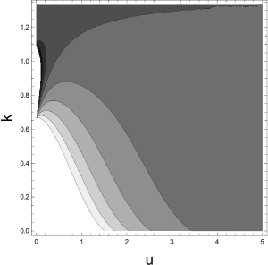
Figure 6: The solutions to the equation (4.17) defined on the region $(0;+\infty)$.

5 Conclusion

In this paper we have analyzed the behaviour of Wilson loops at long distances in the holographic renormalization group flows constructed in [18]. These backgrounds are domain wall and black hole solutions to a 5d dilaton gravity model with an exponential potential. The solutions depend on the parameters $u_{01}$ and $u_{02}$, that yield to different RG flows defined on regions $(u_{01},u_{02})$, $(u_{01},+\infty)$, interpolating between boundaries with hyperscaling violation, and a special case defined on $(u_{0},+\infty)$ ($u_{01}=u_{02}$) with an AdS boundary. We have analyzed holographic rectangular time-like Wilson loops at zero and finite temperatures.

In the case of $T=0$ we have shown that the quark-antiquark potential grows linearly at large $\ell$ for the holographic RG flow defined on domain $(u_{01},u_{02})$, so there is a confinement phase for certain values of the dilaton coupling constant. This is consistent with the observation from [18], where it was seen that the dependence of the running coupling $\lambda=e^{\phi}$ on the energy scale $e^{\mathcal{A}}$ for this RG flow mimics the QCD behaviour. The long distance Wilson loops calculated in two others holographic RG flows at zero temperature have shown that these backgrounds are non-confining. It confirms the observations from [18] where it was pointed the corresponding running couplings of these theories are both UV and IR free.

In the thermal case we have shown that the corresponding RG flow background is in deconfined phase. However, it should be noted that the dependence of the energy scale on the dilaton (see fig. 4) has been indicated that we can not achieve the deep IR.

It would be interesting to perform more careful analysis of the quark-antiquark potential for the confining case. In particular, it is relevant to find out if there any possibility for tuning of the background to reproduce the Cornell potential. Another relevant issue is to compute the Regge spectrum of the holographic mesons. It is also interesting to apply stability analysis to Wilson loop configurations as it was done in [35].

Appendix A Expansion near $u_{02}$ and $u_{01}$

Here we discuss the holographic RG flow (2.3)-(2.4) with $\alpha^{1}=0$ defined on the region $(u_{02},u_{01})$.

$\bullet$ Let us perform expansion of $\mathcal{A}$ end $\phi$ near $u_{02}$.
The scale factor $\mathcal{A}$ (2.10) near $u_{02}$ is

$$\mathcal{A} \sim \frac{4}{(9k^{2}-16)}\log a_{0}-\frac{9k^{2}}{4(9k^{2}-16)}\log(a_{1}(u-u_{02}))+\mathcal{O}((u-u_{02})^{2}),$$ (A.1)

with

$$a_{0}=\sqrt{|\frac{C_{1}}{2E_{1}}|}\sinh(\sqrt{|\frac{3E_{1}}{2}(k^{2}-\frac{16}{9})|}(u_{01}-u_{02})),\quad a_{1}=\frac{2}{3}\sqrt{|C_{2}\frac{9k^{2}-16}{3k^{2}}|}.$$ (A.2)

For the expansion of the dilaton near the point $u_{02}$ we have

$$\phi \sim -\frac{9k}{9k^{2}-16}\log a_{0}+\frac{9k}{9k^{2}-16}\log(a_{1}(u-u_{02}))+\mathcal{O}((u-u_{02})^{2}).$$ (A.3)

Combing the expression for $\mathcal{A}$ and $\phi$ one has

$$e^{3\mathcal{A}} \sim a^{\frac{12}{9k^{2}-16}}_{0}(a_{1}(u-u_{02}))^{-\frac{27k^{2}}{4(9k^{2}-16)}},$$ (A.4)

$$e^{4\mathcal{A}+\frac{8}{3}\phi} \sim a^{\frac{8(2-3k)}{9k^{2}-16}}_{0}\left(a_{1}(u-u_{02})\right)^{\frac{3k(8-3k)}{9k^{2}-16}},$$ (A.5)

$$e^{7\mathcal{A}+\frac{8}{3}\phi} \sim a^{\frac{4(7-6k)}{9k^{2}-16}}_{0}(a_{1}(u-u_{02}))^{\frac{3k(32-21k)}{4(9k^{2}-16)}}.$$ (A.6)

Plugging (A.4)-(A.6) in (3.19)-(1) and integrating one obtains

$$\frac{\mathcal{S}_{NG}}{2} = \frac{a^{\frac{4(7-6k)}{9k^{2}-16}}_{0}(9k^{2}-16)(a_{1}(u_{*}-u_{02}))^{\frac{3(32-21k)k}{36k^{2}-64}+1}\sqrt{a^{\frac{8(2-3k)}{9k^{2}-16}}_{0}(a_{1}(u_{*}-u_{02}))^{\frac{3(8-3k)k}{9k^{2}-16}}-c}\,}{c^{2}(3k-8)(9k-8)}$$ (A.7)

$$\times {\bf{}_{2}F_{1}}\left(1,\frac{5}{4}-\frac{2}{3k};\frac{7}{4}-\frac{2}{3k};\frac{1}{c}a^{\frac{8(2-3k)}{9k^{2}-16}}_{0}(a_{1}(u_{*}-u_{02}))^{\frac{3(8-3k)k}{9k^{2}-16}}\right),$$

while the quark-antiquark distance reads

$$\frac{\ell}{2} = \frac{4(9k^{2}-16)}{c(9k^{2}-64)}a^{\frac{12}{9k^{2}-16}}_{0}(a_{1}(u_{*}-u_{02}))^{\frac{27k^{2}}{64-36k^{2}}+1}\sqrt{a^{\frac{8(2-3k)}{9k^{2}-16}}_{0}(a_{1}(u_{*}-u_{02}))^{\frac{3(8-3k)k}{9k^{2}-16}}-c}\,$$ (A.8)

$$\times {\bf{}_{2}F_{1}}\left(1,\frac{1}{4}-\frac{2}{3k};\frac{3}{4}-\frac{2}{3k};\frac{a^{\frac{8(2-3k)}{9k^{2}-16}}_{0}}{c}(a_{1}(u_{*}-u_{02}))^{\frac{3(8-3k)k}{9k^{2}-16}}\right).$$

$\bullet$ The expansion near $u_{01}$ of the scale factor and the dilaton read

$$\mathcal{A} \sim \frac{4}{(9k^{2}-16)}\log(b_{0}(u-u_{01}))-\frac{9k^{2}}{4(9k^{2}-16)}\log b_{1}+\mathcal{O}((u-u_{01})^{2}),$$ (A.9)

$$\mathcal{\phi} \sim -\frac{9k}{9k^{2}-16}\log(b_{0}(u-u_{01}))+\frac{9k}{9k^{2}-16}\log b_{1}+\mathcal{O}((u-u_{01})^{2}),$$ (A.10)

where

$$b_{0}=\frac{1}{2}\sqrt{3|C_{1}(k^{2}-\frac{16}{9})|},\quad b_{1}=\sqrt{|\frac{C_{2}}{2E_{2}}|}\sinh(\frac{2}{3}\sqrt{\frac{2}{3}}u_{02}\sqrt{|E_{2}(\frac{16}{k^{2}}-9)|}).$$ (A.11)

Then we have

$$e^{3\mathcal{A}} \sim (b_{0}(u-u_{01}))^{\frac{12}{9k^{2}-16}}b_{1}^{-\frac{27k^{2}}{4(9k^{2}-16)}},$$ (A.12)

$$e^{4\mathcal{A}+\frac{8}{3}\phi} \sim (b_{0}(u-u_{01}))^{\frac{8(2-3k)}{9k^{2}-16}}b_{1}^{\frac{3k(8-3k)}{9k^{2}-16}},$$ (A.13)

$$e^{7\mathcal{A}+\frac{8}{3}\phi} \sim (b_{0}(u-u_{01}))^{\frac{4(7-6k)}{9k^{2}-16}}b_{1}^{\frac{3k(32-21k)}{4(9k^{2}-16)}}.$$ (A.14)

Inserting (A.12)-(A.14) in the expression for $\ell$ and integrating one gets (3.19)

$$\frac{\ell}{2} = -\frac{9k^{2}-16}{(9k^{2}-4)b_{0}}b_{1}^{-\frac{27k^{2}}{4(9k^{2}-16)}}(b_{0}(u_{*}-u_{01}))^{\frac{12}{9k^{2}-16}+1}\sqrt{b_{1}^{\frac{3k(8-3k)}{9k^{2}-16}}(b_{0}(u_{*}-u_{01}))^{-\frac{8(3k-2)}{9k^{2}-16}}-1}$$ (A.15)

$$\times {\bf{}_{2}F_{1}}\left(1,\frac{(2-3k)}{8};-\frac{3(k-2)}{8};\frac{1}{c^{2}}b_{1}^{\frac{3k(8-3k)}{9k^{2}-16}}(b_{0}(u_{*}-u_{01}))^{\frac{8(2-3k)}{9k^{2}-16}}\right).$$

Doing the same for the string action $\mathcal{S}_{NG}$ (1) we have

$$\mathcal{S}_{NG} = -\frac{(9k^{2}-16)b_{0}^{\frac{4(7-6k)}{9k^{2}-16}}b_{1}^{\frac{3k(32-21k)}{4(9k^{2}-16)}}}{3(k-2)(3k-2)c}(u_{*}-u_{01})^{\frac{3(k-2)(3k-2)}{9k^{2}-16}}\sqrt{\frac{1}{c^{2}}b_{1}^{\frac{3k(8-3k)}{9k^{2}-16}}(b_{0}(u_{*}-u_{01}))^{-\frac{8(3k-2)}{9k^{2}-16}}-1}\,$$ (A.16)

$$\times {\bf{}_{2}F_{1}}\left(1,\frac{5}{4}-\frac{3k}{8};\frac{7}{4}-\frac{3k}{8};\frac{1}{c^{2}}b_{1}^{\frac{3k(8-3k)}{9k^{2}-16}}(b_{0}(u_{*}-u_{01}))^{\frac{8(2-3k)}{9k^{2}-16}}\right).$$

References

- [1] J.M. Maldacena, The Large limit of superconformal field theories and supergravity, Int. J. Theor. Phys. 38 (1999) 1113, Adv. Theor. Math. Phys. 2 (1998) 23 [hep-th/9711200].
- [2] S.S. Gubser, I.R. Klebanov and A.M. Polyakov, Gauge theory correlators from non-critical string theory, Phys. Lett. B 428 (1998) 105 [hep-th/9802109].
- [3] E. Witten, Anti-de Sitter space and holography, Adv. Theor. Math. Phys. 2 (1998) 253 [hep-th/9802150].
- [4] J. Casalderrey-Solana, H. Liu, D. Mateos, K. Rajagopal, U.A. Wiedemann, Gauge/String Duality, Hot QCD and Heavy Ion Collisions, Cambridge University Press, 2014, [1101.0618[hep-th]].
- [5] I.Ya. Aref’eva, Holographic approach to quark-gluon plasma in heavy ion collisions, Phys. Usp. 57 (2014) 527.
- [6] J. de Boer, E. P. Verlinde and H. L. Verlinde, On the holographic renormalization group, JHEP 0008 (2000) 003; [hep-th/9912012].
- [7] H. J. Boonstra, K. Skenderis and P. K. Townsend, The domain wall/QFT correspondence, JHEP 9901, 003 (1999); [hep-th/9807137].
- [8] M. Bianchi, D. Z. Freedman and K. Skenderis, Holographic renormalization, Nucl. Phys. B 631, 159 (2002); [hep-th/0112119].
- [9] K. Skenderis, Lecture notes on holographic renormalization, Class. Quant. Grav. 19, 5849 (2002); [hep-th/0209067].
- [10] E. T. Akhmedov, A remark on the AdS / CFT correspondence and the renormalization group flow, Phys.Lett. B442 (1998) 152-158;[hep-th/9806217].
- [11] U. Gürsoy, E. Kiritsis, Exploring improved holographic theories for QCD: Part I, JHEP 02 (2008) 032; [0707.1324[hep-th]].
- [12] U. Gürsoy, E. Kiritsis and F. Nitti, Exploring improved holographic theories for QCD: Part II, JHEP 02 (2008) 019; [0707.1349[hep-th]].
- [13] U. Gürsoy, Continuous Hawking-Page transitions in Einstein-scalar gravity, JHEP 01 (2011) 086; [1007.0500[hep-th]].
- [14] M. Järvinen and E. Kiritsis, Holographic Models for QCD in the Veneziano Limit, JHEP 1203 (2012) 002; [1112.1261[hep-th]].
- [15] D. Giataganas, U. Gürsoy and J. F. Pedraza, Strongly-coupled anisotropic gauge theories and holography, Phys. Rev. Lett. 121 (2018) 121601; [1708.05691[hep-th]].
- [16] U. Gürsoy, M. Järvinen, G. Nijs, J. F. Pedraza, Inverse Anisotropic Catalysis in Holographic QCD, JHEP 1904 (2019) 071; [1811.11724[hep-th]].
- [17] I.Ya. Aref’eva, K. Rannu, Holographic anisotropic background with confinement-deconfinement phase transition, JHEP 5 (2018) 206; [arXiv:1802.05652[hep-th]].
- [18] I. Ya. Aref’eva, A.A. Golubtsova and G. Policastro, Exact holographic RG flows and the Toda chain, JHEP 05 (2019) 117 [1803.06764[hep-th]].
- [19] U. Gürsoy, M. Järvinen and G, Policastro, Late time behavior of non-conformal plasmas, JHEP01 (2016) 134 [1507.08628[hep-th]].
- [20] H. Lu, C. N. Pope, E. Sezgin and K. S. Stelle, Dilatonic p-brane solitons, Phys. Lett. B 371, 46 (1996); [/hep-th/9511203].
- [21] E. Kiritsis, W. Li and F. Nitti, Holographic RG flow and the Quantum Effective Action, Fortsch.Phys. 62 (2014) 389-454 (2014); [arXiv:1401.0888[hep-th]].
- [22] J. M. Maldacena, Wilson loops in large field theories, Phys. Rev. Lett. 80 (1998) 4859-4862; [hep-th/9803002].
- [23] S.-J. Rey and J.-T. Yee, Macroscopic strings as heavy quarks in large N gauge theory and anti-de Sitter supergravity, Eur. Phys. J.C 22 (2001) 379-394; [hep-th/9803001].
- [24] S.-J, Rey, S. Theisen, J.-T, Yee, Wilson-Polyakov loop at finite temperature in large N gauge theory and anti-de Sitter supergravity, Nucl.Phys.B 527 (1998) 171-186; [hep-th/9803135].
- [25] A. Brandhuber, N. Itzhaki, J. Sonnenschein, S. Yankielowicz, Wilson loops, confinement, and phase transitions in large N gauge theories from supergravity, JHEP 9806 (1998) 001; [hep-th/9803263].
- [26] J. Distler and F. Zamora, Non-Supersymmetric Conformal Field Theories from Stable Anti-de Sitter Spaces,Adv. Theor. Math. Phys.2 (1999) 1405; [hep-th/9810206].
- [27] L. Girardello, M. Petrini, M. Porrati and A. Zaffaroni, Confinement and Condensates Without Fine Tuning in Supergravity Duals of Gauge Theories, JHEP 9905 (1999) 026; [hep-th/9903026].
- [28] L. Girandello, M. Petrini, M. Poratti and A. Zaffaroni, The Supergravity dual of N=1 superYang-Mills theory, Nucl.Phys. B569 (2000) 451-469; [hep-th/9909047].
- [29] M. Petrini, A. Zaffaroni, The Holographic RG flow to conformal and nonconformal theory, PoS tmr99 (1999) 053; [hep-th/0002172].
- [30] I.Ya. Aref’eva, K. Rannu, P. Slepov, Orientation Dependence of Confinement-Deconfinement Phase Transition in Anisotropic Media, Phys. Lett. B 792 (2019) 470-475; [arXiv:1808.05596[hep-th]].
- [31] J. Casalderrey-Solana, D. Gutiez, C. Hoyos, Effective long distance potential in holographic RG flows, JHEP 04 (2019)134; [arXiv:1902.04279[hep-th]].
- [32] I.Ya. Aref’eva, Holography for Heavy Ions Collisions at LHC and NICA, EPJ Web Conf. 164 (2017) 01014 (2017); [1612.08928[hep-th]].
- [33] D. Giataganas, Probing strongly coupled anisotropic plasma, JHEP 1207 (2012) 031; [arXiv:1202.4436[hep-th]].
- [34] S.S. Gubser, Curvature singularities: The Good, the bad and the naked,Adv. Theor. Math. Phys. 4 (2000) 679 ; [arXiv:0002160[hep-th]].
- [35] Raúl E. Aria and Guillermo A. Silva, Wilson loops stability in the gauge/string correspondence, JHEP 01(2010) 023; [arXiv: 0911.0662[hep-th]].