Consensus Monte Carlo for Random Subsets using Shared Anchors

Abstract

We present a consensus Monte Carlo algorithm that scales existing Bayesian nonparametric models for clustering and feature allocation to big data. The algorithm is valid for any prior on random subsets such as partitions and latent feature allocation, under essentially any sampling model. Motivated by three case studies, we focus on clustering induced by a Dirichlet process mixture sampling model, inference under an Indian buffet process prior with a binomial sampling model, and with a categorical sampling model. We assess the proposed algorithm with simulation studies and show results for inference with three datasets: an MNIST image dataset, a dataset of pancreatic cancer mutations, and a large set of electronic health records (EHR). Supplementary materials for this article are available online.

Keywords: Big data, electronic health records, image cluster, parallel computing, tumor heterogeneity,

1 Introduction

We develop a consensus Monte Carlo (CMC) algorithm for Bayesian nonparametric (BNP) inference with large datasets that are too big for full posterior simulation on a single machine, due to CPU or memory limitations. The proposed algorithm is for inference under BNP models for random subsets, including clustering, feature allocation (FA), and related models. We distribute a large dataset to multiple machines, run separate instances of Markov chain Monte Carlo (MCMC) simulations in parallel and then aggregate the Monte Carlo samples across machines. The idea of the proposed CMC hinges on choosing a portion of observations as anchor points (Kunkel and Peruggia, , 2018) which are distributed to every machine along with other observations that are only available to one machine. Those anchor points then serve as anchors to merge Monte Carlo draws of clusters or features across machines.

Clustering is an unsupervised learning method that partitions observations into non-overlapping subsets (clusters) with the aim of creating homogeneous groups. A widely used approaches for model-based inference on random partitions is based on mixtures, with each mixture component being a cluster. Bayesian finite mixture models with a random number of terms that allow for inference with an a priori unknown number of clusters, is first discussed in Richardson and Green, (1997). A natural generalization of such models are infinite mixtures with respect to discrete random probability measures. In fact, any exchangeable random partition can be represented this way (Kingman, , 1978). Prior probability models for random probability measures, such as the mixing measure in this representation, are known as BNP models. Examples include Dirichlet process mixtures (DPM, Lo, 1984; MacEachern, 2000; Lau and Green, 2007), Pitman-Yor process mixtures (Pitman and Yor, , 1997) and variations with different data structures, such as Rodriguez et al., (2011) for mixtures of graphical models, normalized inverse Gaussian process mixtures (Lijoi et al., , 2005), normalized generalized Gamma process mixtures (Lijoi et al., , 2007), and more general classes of BNP mixture models (Barrios et al., , 2013; Favaro and Teh, , 2013; Argiento et al., , 2010). For a more general discussion of BNP priors on random partitions see also de Blasi et al. (2015).

Feature allocation, also known as overlapping clustering, relaxes the restriction to mutually exclusive and non-overlapping subsets and allocates each observation to possibly more than one subset (“feature”). The most commonly used feature allocation model is the Indian buffet process (IBP, Ghahramani and Griffiths, 2006; Broderick et al., 2013a ; Broderick et al., 2013c ).

A convenient way to represent random subsets, in clustering as well as in feature allocation, is as a binary matrix $\bm{A}$ with $A_{ik}=1$ indicating that experimental unit $i$ is a member in the $k$-th random subset. Feature allocation for $n$ experimental units into an unknown number $K$ of subsets then takes the form of a prior $p(\bm{A})$ for a random binary $(n\times K$) matrix $\bm{A}$ with a random number of columns. Similarly, a random partition becomes a prior $p(\bm{A})$ with exactly one non-zero element in each row, and a random number $K$ of columns, $1\leq K\leq n$. An important feature of BNP clustering and feature allocation models is that they do not require an a prior specification of the number of subsets, (clusters or features). An important limitation is the requirement for intensive posterior simulation. Implementation of posterior inference by MCMC simulation is usually not scalable to large datasets.

Several approaches have been proposed to overcome these computational limitations in general big-data problems, not necessarily restricted to BNP models. Huang and Gelman, (2005) proposed CMC algorithms that distribute data to multiple machines, each of which runs a separate MCMC simulation in parallel. Various ways of consolidating simulations from these local posteriors have been proposed. Scott et al., (2016) combined the local posterior draws by weighted averages. Neiswanger et al., (2013) and White et al., (2015) proposed parametric, semiparametric and nonparametric approaches to approximate the full posterior density as the product of local posterior densities. Wang and Dunson, (2013) introduced the Weierstrass sampler which applies a Weierstrass transform to each local posterior. Minsker et al., (2014) found the geometric median of local posterior distributions using a reproducing kernel Hilbert space embedding. Rabinovich et al., (2015) proposed a variational Bayes algorithm that optimizes over aggregation functions to achieve a better approximation to the full posterior. Recently, Entezari et al., (2018) introduced the likelihood inflating sampling algorithm (LISA) as a clever alternative to CMC. Instead of raising the prior to a fractional power as in CMC, LISA inflates the likelihood so that each local posterior is a close representation of the whole-data posterior. All but the method by Rabinovich et al., (2015) are specifically designed to aggregate global parameters. However, local parameters i.e., parameters that are indexed by experimental units, such as cluster assignment and latent feature allocation are also of great importance in big data analytics. Even though the method by Rabinovich et al., (2015) can be used to aggregate local structures such as cluster assignment, it assumes the number of clusters is fixed a priori, which limits it applicability. Our contribution is to bridge this gap in the literature.

Blei et al., (2006) developed the first variational Bayes algorithm for posterior inference of DPM which was later extended to several variational algorithms by Kurihara et al., (2007). A similar variational Bayes algorithm for posterior inference under an IBP prior was derived by Doshi-Velez et al., 2009a . Doshi-Velez et al., 2009b propose a parallel MCMC algorithm which relies on efficient message passing between the root and worker processors. Wang and Dunson, (2011) developed a single-pass sequential algorithm for conjugate DPM models. In each iteration, they deterministically assign the next subject to the cluster with the highest probability conditional on past cluster assignments and data up to the current observation. Rai and Daume, (2011) developed a beam-search heuristic to perform approximate maximum a posteriori inference for linear-Gaussian models with IBP prior. Under the same model, Reed and Ghahramani, (2013) proposed a greedy maximization-expectation algorithm, a special case of variational Bayes algorithm, which exploits the submodularity of the evidence lower bound. Broderick et al., 2013b and Xu et al., (2015) develop small-variance asymptotics for approximate posterior inference under an IBP prior. Lin, (2013) proposed a one-pass sequential algorithm for DPM models. The algorithm utilizes a constructive characterization of the posterior distribution of the mixing distribution given data and a partition. Variational inference is adopted to sequentially approximate the marginalization. Williamson et al., (2013) introduced a parallel MCMC for DPM models which involves iteration over local updates and a global update. For the local update, they exploit the fact that a Dirichlet mixtures of Dirichlet processes (DP) again defines a DP, if the parameters of Dirichlet mixture are suitably chosen. Ge et al., (2015) used a similar characterization of the DP as in Lin, (2013). But instead of a variational approximation, they adapted the slice sampler for parallel computing under a MapReduce framework. Tank et al., (2015) developed two variational inference algorithms for general BNP mixture models. Recently, Zuanetti et al., (2019) suggested two efficient alternatives using DPM with conjugate priors. The first approach is based on a predictive recursion algorithm (Newton et al., , 1998) which requires only a single scan of all observations and avoids expensive MCMC. The second approach is a two-step MCMC algorithm. It first distributes data onto different machines and computes clusters locally in parallel. A second step combines the local clusters into global clusters. All steps are carried out using MCMC simulation under a common DPM model. Ni et al., 2019a extended the second approach to non-conjugate models.

We propose a new CMC algorithm specifically for aggregating subject-specific latent combinatorial structures that often arise from BNP models. The proposed CMC algorithm is applicable to both clustering and feature allocation problems. It uses a similar notion, anchor points, as in Kunkel and Peruggia, (2018) but with a completely different purpose. In Kunkel and Peruggia, (2018), they used anchor points to address label switching in finite Gaussian mixture models whereas in this paper, we use anchor points to combine posterior draws of random clusters or features across different shards of the original data. The proposed CMC can reduce the computation cost by at least a factor of $S$ where $S$ is the number of computing cores at disposal. Since modern high performance computing centers typically have tens of thousands to hundreds of thousands computing cores in total, $S$ is easily in the order of thousands.

The rest of this article is organized as follows. We provide relevant background for CMC and two BNP models in Section 2. The proposed CMC is introduced in Section 3. The utility of the proposed CMC is demonstrated with simulation studies in Section 4 and three real applications in Section 5. We conclude the paper by a brief discussion in Section 6.

2 Background

CMC schemes are algorithms to generate approximate posterior Monte Carlo samples given a large dataset. The idea of CMC can be summarized in three steps: (i) distribute a large dataset to multiple machines (shards); (ii) run separate MCMC algorithm on each machine without any inter-machine communication; and (iii) aggregate Monte Carlo samples across machines to construct consensus posterior samples. Step (iii) is non-trivial.

Let $\bm{y}$ denote the full dataset and let $\bm{y}_{s}$ denote shard $s$ for $s=1,\dots,S$. And let $\bm{\theta}$ denote the global parameters. Assuming $\bm{y}$ to be exchangeable, the posterior distribution can be written as

$$p(\bm{\theta}\mid\bm{y})\propto p(\bm{y}\mid\bm{\theta})p(\bm{\theta})=\prod_{s=1}^{S}p(\bm{y}_{s}\mid\bm{\theta})p(\bm{\theta})^{1/S}$$ (1)

where the fractional prior preserves the total amount of prior information. Expression (1) is exact and involves no approximation. Ideally, if one can compute $p(\bm{y}_{s}\mid\bm{\theta})p(\bm{\theta})^{1/S}$ analytically for each shard $s$, then (1) can be directly used to obtain the posterior distribution based on the entire dataset. However, $p(\bm{y}_{s}\mid\bm{\theta})p(\bm{\theta})^{1/S}$ is usually not analytically available and only Monte Carlo samples are returned from step (ii), which necessitates step (iii).

Various methods have been proposed to aggregate Monte Carlo samples such as weighted averaging (Scott et al., , 2016), density estimation (Neiswanger et al., , 2013; White et al., , 2015), geometric median (Minsker et al., , 2014) and a variational algorithm (Rabinovich et al., , 2015). One common limitation of existing approaches is that they cannot aggregate Monte Carlo samples of subject-specific latent structure (e.g. cluster assignment and feature allocation) that often arise in posterior inference under BNP models. For example, in a feature allocation problem each shard introduces new, additional feature memberships. That is, $\bm{\theta}$ could be partitioned as $\bm{\theta}=(\bm{\theta}_{s},s=1,\ldots,S)$, with each shard adding an additional set of parameters $\bm{\theta}_{s}$.

BNP models are Bayesian models defined on an infinite-dimensional parameter space. Common examples of BNP models include the DPM model for clustering and the IBP prior for feature allocation. The main attraction of BNP models are flexible modeling and the full prior support in many models. For example, DP and IBP can automatically select the number of clusters and features based on available data. As examples illustrating the proposed CMC algorithm, we consider applications of the DPM model and the IBP model in three different inference problems. The inference problems are clustering, using a DP prior; FA, using an IBP prior; and double feature allocation (DFA, Ni et al., 2019), using an IBP prior. For the implementation we use the R packages DPpackage and dfa. Next we introduce some notations by way of a brief review of the three models and the inference problems.

2.1 Dirichlet process mixtures and random partitions

Let $\bm{y}_{1},\dots,\bm{y}_{n}$ denote data observed on experimental units $i=1,\ldots,n$. Some applications call for clustering, i.e., a partition of $[n]\equiv\{1,\ldots,n\}$ into $[n]=\bigcup_{k=1}^{K}F_{k}$, with $F_{k}\cap F_{k^{\prime}}=\emptyset$ for $k\not=k^{\prime}$. A widely used model-based approach to implement inference on the unknown partition is to assume i.i.d. sampling from a mixture model, $\bm{y}_{i}\sim\int f(\bm{y}_{i}\mid\bm{\theta})\;dG(\bm{\theta})$. Here $f(\bm{y}\mid\bm{\theta})$ is, for example, a normal distribution with location $\bm{\theta}$ (leaving the scale parameter as an additional hyperparameter), and $G(\cdot)=\sum_{h}w_{h}\delta_{m_{h}}(\cdot)$ is a discrete mixing measure. Introducing latent variables $\bm{\theta}_{i}$, the model can equivalently be written as a hierarchical model

$$\bm{y}_{i}\mid\bm{\theta}_{i}\sim f(\bm{y}_{i}\mid\bm{\theta}_{i})\mbox{ and }\bm{\theta}_{i}\sim G.$$ (2)

The discrete nature of $G$ gives rise to ties among the $\bm{\theta}_{i}$, which in turn naturally define the desired partition of $[n]$. Assume there are $K$ unique values, denoted by $\bm{\theta^{\star}}=\{\bm{\theta^{\star}}_{1},\ldots,\bm{\theta^{\star}}_{K}\}$, and define clusters $F_{k}=\{i:\;\bm{\theta}_{i}=\bm{\theta^{\star}}_{k}\}$. Sometimes it is more convenient to alternatively represent the partition using cluster membership indicators $s_{i}=k$ if $i\in F_{k}$. Yet another alternative representation, that will be useful later, is using binary indicators $A_{ik}$ with $A_{ik}=1$ if $i\in F_{k}$. Collecting all indicators in an $(n\times K)$ binary matrix $\bm{A}=[A_{ik}]$, the constraint to non-overlapping subsets becomes $\sum_{k}A_{ik}=1$ for all rows $i=1,\ldots,n$.

Model (2) is completed with a BNP prior on $G$, for example, $G\sim\mbox{DP}(m,G_{0}),$ where $\mbox{DP}(m,G_{0})$ denotes a DP prior with concentration parameter $m$ and base measure $G_{0}$. Model (2) with the DP hyperprior on $G$ defines the DPM model. See, for example, Ghoshal, (2010) for a good review. The implied distribution $p(\bm{F})$ over partitions $\bm{F}=\{F_{1},\ldots,F_{K}\}$ under a DPM model is known as the Chinese restaurant process. Inference on the random partition is straightforward to implement through, for example, Algorithm 8 in Neal, (2000). Neal’s algorithm 8 iterates between two steps: (i) For $i=1,\dots,n$, sample $s_{i}$ given the $i$th observations $\bm{y}_{i}$, cluster-specific parameters $\bm{\theta}_{1}^{\star},\dots,\bm{\theta}_{K}^{\star}$, and cluster assignments $\bm{s}_{-i}$ for the rest of the observations. (ii) For $k=1,\dots,K$, sample $\bm{\theta}_{k}^{\star}$ given data $\bm{y}_{1},\dots,\bm{y}_{n}$ and cluster assignments $s_{1},\dots,s_{n}$.

2.2 Indian buffet process and feature allocation

The IBP is a BNP prior for random subsets $\bm{F}=\{F_{k}\subseteq[n];\;k=1,\ldots,K\}$ that can possibly overlap and need not be exhaustive, i.e, without the restrictions of a partition. Again, the number $K$ of random subsets is random. The subsets are known as features. A prior $p(\bm{F})$ defines a random feature allocation model (Broderick et al., 2013a, ). Similar to before, we can alternatively represent the feature allocation with feature membership indicators, $A_{ik}=1$ if $i\in F_{k}$, now without the constraint to unit row sums. The columns of $\bm{A}=[A_{ik}]$ represent the features $F_{1},\ldots,F_{K}$.

Xu et al., (2015) use random feature allocation to develop inference for tumor heterogeneity, i.e., the deconvolution of a heterogeneous population of tumor cells into latent homogeneous subclones (i.e. cell subtypes). The experiment records short reads counts of $n$ single nucleotide variants (SNVs) (essentially, mutations relative to a given reference) in tumor tissues $j=1,\ldots,p$. The hypothesized homogeneous subclones are charecterized by the presence or absence of these SNVs. In this application, $A_{ik}=1$ if SNV $i$ is present in subclone $k$. Let $y_{ij}$ denote the observed counts of SNV $i$ in sample $j$ and let $N_{ij}$ denote the total counts at locus $i$. Let $\theta^{\star}_{jk}$ denote the unknown proportion of subclone $k$ in tumor $j$. The experimental setup implies independent binomial sampling, for $i=1,\dots,n$ and $j=1,\dots,p$,

$$y_{ij}\sim\mbox{Bin}(N_{ij},p_{ij})\mbox{~{}~{}with~{}~{}}p_{ij}=b_{j}p_{0}+\sum_{k=1}^{K}\theta^{\star}_{jk}A_{ik},$$ (3)

where $p_{0}$ is the relative frequency of a SNV in the background and $\bm{\theta^{\star}}_{k}=(\theta^{\star}_{jk},\;j=1,\ldots,p)$ are feature-specific parameters. The model is completed with a Dirichlet prior on $(b_{j},\theta^{\star}_{j1},\ldots,\theta^{\star}_{jK})$, a beta prior on $p_{0}$ and a prior on the feature allocation $p(\bm{A})$.

The most widely used prior $p(\bm{A})$ for feature allocation is the IBP. It defines a prior distribution for an $(n\times K)$ binary matrix $\bm{A}=[A_{ik}]$ with a random number of columns. We start the model construction assuming a fixed number $K$ of features, to be relaxed later. Conditional on $K$, $A_{ik}$’s are assumed to be independent Bernoulli random variables, $A_{ik}\mid\pi_{k}\sim Ber(\pi_{k})$ with $\pi_{k}$ following a conjugate beta prior, $\pi_{k}\sim Beta(m/K,1)$. Here $m$ is a fixed hyperparameter. Marginalizing out $\pi_{k}$,

$$p(\bm{A})=\prod_{k=1}^{K}\frac{m\Gamma(c_{k}+\frac{m}{K})\Gamma(n-c_{k}+1)}{K\,\Gamma(n+1+\frac{m}{K})},$$

where $c_{k}=\sum_{i=1}^{n}A_{ik}$ is the sum of the $k$th column of $\bm{A}$.

Let $H_{n}=\sum_{i=1}^{n}1/i$ be the $n$-th harmonic number. Next, take the limit $K\rightarrow\infty$ and remove columns of $\bm{A}$ with all zeros. Let $K^{+}$ denote the number of non-empty columns. The resulting matrix $\bm{A}$ follows an $\mbox{IBP}(m)$ prior (without a specific column ordering), with probability

$$p(\bm{A})=\frac{m^{K^{+}}\exp\{-mH_{n}\}}{K^{+}!}\prod_{k=1}^{K^{+}}\frac{\Gamma(c_{k})\Gamma(n-c_{k}+1)}{\Gamma(n+1)}.$$ (4)

With a finite sample size, the number $K^{+}$ of non-empty columns is finite almost surely. Let $r_{-i,k}$ denote the sum in column $k$, excluding row $i$. Then the conditional probability for $A_{ik}=1$ is

$$p(A_{ik}=1\mid\bm{A}_{-i,k})=r_{-i,k}/n,$$ (5)

provided $r_{-i,k}>0$, where $\bm{A}_{-i,k}$ is the $k$-th column of $\bm{A}$ excluding $i$-th row. And the distribution of the number of new features (non-empty columns) for each row is $\mbox{Poi}(m/n)$. Posterior inference can be carried out using an algorithm similarly to Neal’s algorithm 8. The posterior distribution may present many peaked modes for moderate to large total counts $N_{ij}$, which makes MCMC inefficient. To improve mixing, Ni et al., 2019b used parallel tempering to flatten the posterior while still targeting the right posterior distribution. We will follow their strategy in MCMC.

2.3 Double feature allocation

Some applications call for simultaneous clustering of rows and columns of a data matrix. This is known as bi-clustering (Hartigan, , 1972). Ni et al., (2019) introduces a similar prior model for random row and column subsets, but now without the restrictions of a partition, i.e., random feature allocation on rows and columns simultaneously. Figure 1 illustrates how matching pairs $(F_{k},R_{k})$ of subsets $F_{k}\subseteq[n]$ and $R_{k}\subseteq[p]$ define a disease in electronic health records (EHR) data. The data is an $(n\times p)$ matrix $\bm{Y}=[y_{ij}]$ of recorded symptoms, $j=1,\ldots,p$, on patients $i=1,\ldots,n$.

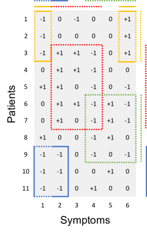
Figure 1: Double feature allocation: simultaneous feature allocation on rows (patients) and columns (symptoms) defines diseases. The data are recorded symptoms, $j=1,\ldots,p$, for patients, $i=1,\ldots,n$, in electronic health records (EHR) data. Each subset $F_{k}$ of patients and matching subset $R_{k}$ of symptoms is a different disease, marked by different boxes. The data $(n\times p)$ matrix $\bm{Y}=[y_{ij}]$ records trinary symptoms with possible outcomes $\{-1,0,1\}$.

A prior on random pairs $(F_{k},R_{k})$ of matching subsets defines a double feature allocation (DFA, Ni et al., 2019). A simple extension of a feature allocation model, such as the IBP, can be used to define a DFA. Let $\bm{A}$ denote a matrix of feature membership indicators for the subsets $F_{k}\subseteq[n]$, as before. We first assume $\bm{A}\sim\mbox{IBP}(m)$. In particular, $p(\bm{A})$ induces a prior on the number of subsets $K$. Conditional on $\bm{A}$ we then define a second membership matrix $\bm{C}$, for membership in matched subsets $R_{k}\subseteq[p]$. Here $\bm{C}=[C_{jk}]$ with $C_{jk}$ recording membership of column $j$ in $R_{k}$. In anticipation of the upcoming sampling model for trinary symptoms, $y_{ij}\in\{-1,0,1\}$, we allow for membership $C_{jk}\in\{-1,0,1\}$, with $-1$ indicating that disease $k$ favors symptom $j$ at level $-1$ (e.g., low blood pressure), $1$ indicating that the symptom is favored at level $1$ (e.g., high blood pressure), and $0$ indicating that the symptom is not related to disease $k$. Let $\bm{\pi}=(\pi_{-1},\pi_{0},\pi_{1})$ denote a probability vector. We assume $p(C_{jk}=c)=\pi_{c}$, with a conjugate hyperprior $\bm{\pi}\sim Dir(a_{-1},a_{0},a_{1})$. We assume conditionally independent trinary latent logistic regression as a sampling model for the observed symptoms $y_{ij}\in\{-1,0,1\}$ for patient $i$,

$$p(y_{ij}=y\mid\bm{A},\bm{\theta^{\star}},\bm{\eta})\propto\begin{cases}e^{\eta_{j}^{-}+\sum_{k=1}^{K}w_{jk}^{-}\,I(A_{ik}=1,C_{jk}=-1)}&\mbox{if~{}~{}}y=-1\\ 1&\mbox{if~{}~{}}y=0\\ e^{\eta_{j}^{+}+\sum_{k=1}^{K}w_{jk}^{+}\,I(A_{ik}=1,C_{jk}=1)}&\mbox{if~{}~{}}y=1\end{cases}$$ (6)

where $(w_{jk}^{+},w_{jk}^{-},\;j=1,\ldots,p)$ are feature-specific weights, and $\bm{\eta}=(\eta_{j}^{-},\eta_{j}^{+})$ are symptom-specific offsets. The model is completed with priors for the hyperparameters, $\eta_{j}^{-}$, $\eta_{j}^{+}\sim N(0,\tau^{2})$ and $w_{jk}^{-}$, $w_{jk}^{+}\sim Ga(1,\tau_{w})$. In model (6) the feature-specific parameters are $\bm{\theta^{\star}}_{k}=(C_{jk},w_{jk}^{+},w_{jk}^{-};\;j=1,\ldots,p)$ for feature $F_{k}$. Recognizing the columns of $\bm{C}$ as just another part of feature-specific parameters $\bm{\theta^{\star}}_{k}$ reveals the nature of the DFA model as a special case of a feature allocation, with one of the feature-specific parameters selecting a matching subset of the columns in the data matrix.

Straightforward modifications define similar models for categorical data with fewer or more categories. Posterior inference can be carried out using an algorithm similarly to Neal’s algorithm 8; see Ni et al., (2019) for implementation details.

3 A consensus Monte Carlo algorithm for random subsets

We describe the proposed CMC algorithm in its general form. Let $y_{1},\dots,y_{n}$ denote the data of $n$ observations. Let $\bm{A}=[A_{ik}]$ denote the latent subset membership matrix (for clusters, features, or row-features in random partitions, FA, and DFA, respectively) where $A_{ik}=1$ if observation $i$ belongs to subset $k$. Let $\bm{A}_{i}$ be the $i$-th row of $\bm{A}$. Let $\bm{\theta^{\star}}=\{\bm{\theta^{\star}}_{1},\bm{\theta^{\star}}_{2},\cdots\}$ denote an infinite sequence of subset-specific parameters and let $\bm{\theta}_{\bm{A}_{i}}$ denote a subsequence indexed by $\bm{A}_{i}$, i.e. $\bm{\theta}_{\bm{A}_{i}}=\{\bm{\theta^{\star}}_{k}\mid A_{ik}=1\}$. Many BNP models including DPM, FA, and DFA models can be generically written as a hierarchical model,

$$y_{i}\mid\bm{\theta^{\star}},\bm{A}_{i} \stackrel{{\scriptstyle\mbox{\scriptsize ind}}}{{\sim}} p(y_{i}\mid\bm{\theta}_{\bm{A}_{i}})$$

$$\bm{\theta^{\star}}_{k}\mid\bm{A} \stackrel{{\scriptstyle\mbox{\scriptsize iid}}}{{\sim}} \pi_{\theta}(\cdot)$$

$$\bm{A}=[\bm{A}_{1}\;\cdots\bm{A}_{n}]^{\prime} \sim \pi_{\bm{A}}(\cdot)$$ (7)

for $i=1,\dots,n$ and $k=1,2,\ldots$. The sampling model for $y_{i}$ in the first line depends on the specific inference model. In the case of a random partition it is the kernel of the mixture model in (2). In the case of an FA or DFA model the sampling model might include multiple $\bm{\theta^{\star}}_{k}$ when $\sum_{k}A_{ik}>1$, as in (3) or (6). The specific interpretation is problem-specific. The dependence on $\bm{A}$ in the second line is only indirect through the random number of columns in $\bm{A}$ which defines the number of subsets. In DPM models, $\pi_{\theta}(\cdot)=G_{0}$ is the baseline distribution and $\pi_{\bm{A}}(\cdot)$ is the Chinese restaurant process. In FA and DFA models, $\pi_{\theta}(\cdot)$ is the prior of feature-specific parameters and hyperparameters, and $\pi_{\bm{A}}(\cdot)$ is the IBP.

For a small to moderate sample size $n$, MCMC has been commonly used to implement posterior inference. However, when $n$ is large, MCMC becomes computationally prohibitive because at each iteration, it has to scan through all observations. The idea of CMC is to distribute the large dataset onto many shards so that MCMC can be efficiently implemented on each shard with much smaller sample size. Let $S$ be a large integer. We randomly divide the observations into $(S+1)$ non-overlapping shards $\bm{i}_{s}\subset\{1,\dots,n\}=\cup_{s=1}^{S+1}\bm{i}_{s}$ and $\bm{y}_{s}=\{y_{i}:\;i\in\bm{i}_{s}\}$. Define $\widetilde{\bm{y}}_{s}=\bm{y}_{s}\cup\bm{y}_{S+1}$ for $s=1,\dots,S$, so that $\{\widetilde{\bm{y}}_{s}\}$ are new shards that all share $\bm{y}_{S+1}$ but are otherwise disjoint. We call $\bm{y}_{S+1}$ the anchor points. Let $\{\bm{\theta}_{s}^{(t)},\bm{F}_{s}^{(t)}\}_{t=1}^{T}=MCMC(\widetilde{\bm{y}}_{s})$ where $\bm{F}_{s}^{(t)}=\{F_{sk}^{(t)}\}_{k=1}^{K_{s}^{(t)}}$ denote $T$ Monte Carlo samples obtained from the MCMC algorithm applied to the shard $\widetilde{\bm{y}}_{s}$. To aggregate the Monte Carlo samples from shards $s$ and $s^{\prime}$, we consider merging (i.e. taking the union of) two clusters or features $F_{sk}^{(t)}$ and $F_{s^{\prime}k^{\prime}}^{(t)}$ if

$$d_{sk,s^{\prime}k^{\prime}}^{(t)}=\frac{D(F_{sk}^{(t)},F_{s^{\prime}k^{\prime}}^{(t)})}{C(F_{sk}^{(t)},F_{s^{\prime}k^{\prime}}^{(t)})+D(F_{sk}^{(t)},F_{s^{\prime}k^{\prime}}^{(t)})}<\epsilon,$$ (8)

where $D(F_{sk}^{(t)},F_{s^{\prime}k^{\prime}}^{(t)})$ is the number of different elements in $F_{sk}^{(t)}\cap\bm{i}_{S+1}$ and $F_{s^{\prime}k^{\prime}}^{(t)}\cap\bm{i}_{S+1}$ and $C(F_{sk}^{(t)},F_{s^{\prime}k^{\prime}}^{(t)})$ is the number of common elements. By convention, we set $d_{sk,s^{\prime}k^{\prime}}^{(t)}=1$ if $C(F_{sk}^{(t)},F_{s^{\prime}k^{\prime}}^{(t)})=D(F_{sk}^{(t)},F_{s^{\prime}k^{\prime}}^{(t)})=0$. In words, if two random subsets (clusters or features) have similar sets of anchor points, we merge them. The similarity is controlled by the tuning parameter $\epsilon$ which is a small fixed constant. Consider a toy example with 8 data points $\{1,\dots,8\}$. We assign $\{1,2\}$ to shard $s=1$, $\{3,4\}$ to shard $s=2$, and $\{5,6,7,8\}$ as anchor points. Suppose $F_{11}=\{1,5,6,7,8\}$, $F_{12}=\{2,8\}$, $F_{21}=\{3,4,5,6,7\}$ and $F_{22}=\{3,6,8\}$. Using $\epsilon=0.3$, we will merge $F_{11}$ and $F_{21}$ into $F^{\star}=F_{11}\cup F_{21}=\{1,3,4,5,6,7,8\}$, but keep $F_{12}$ and $F_{22}$ unchanged. The choice of (8) includes arbitrary choices. In particular, we note that, for example, the IBP includes positive prior probability for two identical columns in $\bm{A}$, which could question the appearance of identical subsets of anchor points as a criterion for merging. However, in most applications, including the two motivating applications related to feature allocation in this article, this is not a desirable feature of the IBP, and we argue that the criterion introduces an even desirable approximation. Alternatively, the criterion could include a comparison of feature-specific parameters $\bm{\theta^{\star}}_{k}$. In simulation studies and the motivating applications we found the proposed criterion to work well, and prefer the simplicity of (8). We also find that the proposed algorithm is relatively robust with respect to the choice of $\epsilon$ (see Section 5.1 for sensitivity analysis) if the number $|\bm{i}_{S+1}|$ of anchor points is sufficiently large.

If we decide to merge $F_{sk}^{(t)}$ and $F_{s^{\prime}k^{\prime}}^{(t)}$, we merge the associated parameters $\bm{\theta}_{sk}^{\star(t)}$ and $\bm{\theta}_{s^{\prime}k^{\prime}}^{\star(t)}$ according to the following operation. For categorical parameters, such as column $k$ of $\bm{C}_{jk}$ in (6), a majority vote is used, weighted by the relative sizes of the two merged random subsets. For continuous parameters that index a sampling model, such as in (2), the values are averaged, again based on the relative subet sizes. The weighted average is valid only when the support of the parameter is a convex set, which is true in most applications including all our examples. When the support is not convex (e.g. weighted directed acyclic graphs), alternative merging operations need to be designed on a case-by-case basis. Note that the aggregating step is trivially parallelizable with respect to the number $T$ of Monte Carlo samples and hence the computation time is negligible compared to MCMC. The complete CMC is summarized in Algorithm 1. In the algorithm, parfor indicates a parallel loop, while for indicates a sequential loop.

Algorithm 1

1:Data preparation. Split data into $S+1$ disjoint shards $\bm{i}_{s}\subset\{1,\dots,n\}=\cup_{s=1}^{S+1}\bm{i}_{s}$. Form $S$ shards: $\widetilde{\bm{y}}_{s}=\bm{y}_{s}\cup\bm{y}_{S+1}$ for $s=1,\dots,S$. Anchor points $\bm{y}_{S+1}$ are present in every shard, whereas $\bm{y}_{s}$ only appear in shard $s$.

2:parfor $s=1,\dots,S$  do

3:     $\{\bm{\theta}_{s}^{(t)},\bm{F}_{s}^{(t)}\}_{t=1}^{T}=MCMC(\widetilde{\bm{y}}_{s})$

4:end parfor

5:parfor $t=1,\dots,T$ do

6:     randomly permutate the order of the shards

7:     for each pair of pairs $(s,k)$ and $(s^{\prime},k^{\prime})$, $s^{\prime}>s$ do

8:         if $d_{sk,s^{\prime}k^{\prime}}^{(t)}<\epsilon$ then

9:              merge $F_{sk}^{(t)}$ and $F_{s^{\prime}k^{\prime}}^{(t)}$

10:              merge $\bm{\theta}_{sk}^{\star(t)}$ and $\bm{\theta}_{s^{\prime}k^{\prime}}^{\star(t)}$

11:         end if

12:     end for

13:end parfor

14:Output: $\{\bm{\theta}^{(t)},\bm{F}^{(t)}\}_{t=1}^{T}$

We implement the algorithm in the upcoming simulation studies, and in the motivating applications in the context of DPM models and FA and DFA based on IBP models. However, the approach is more general. It remains valid for any alternative BNP prior on $G$ in (2), and any alternative FA prior. For example, the BNP prior could be any other random discrete probability measure, including a normalized completely random measure as in Barrios et al., (2013); Favaro and Teh, (2013) or Argiento et al., (2010). The IBP could be replaced by any other random feature allocation (Broderick et al., 2013c, ). Also, the sampling models in (2), (3) and (6) are examples. Any other sampling model could be substituted, including a regression on additional covariates, or, in the case of feature allocation, a linear-Gaussian model. While we use it here only for BNP models, the same algorithm can be implemented for inference under any parametric model for random subsets, for example, finite mixture models or finite feature allocation models.

We propose a simple diagnostic to summarize the level of approximation in the CMC. First select any two shards, without loss of generality assuming they are $\bm{i}_{1}$ and $\bm{i}_{2}$. We then apply CMC with $\bm{i}_{S+1}$ as anchor points. Denote the point estimate of random subsets (e.g. clusters, latent features) by $\widehat{\bm{A}}_{\mbox{\tiny CMC}}$. In addition, we run a full MCMC simulation in $\bm{i}_{1}\cup\bm{i}_{2}\cup\bm{i}_{S+1}$ and denote the point estimate by $\widehat{\bm{A}}_{\mbox{\tiny MCMC}}$. We summarize the level of the approximation by measuring the distance between $\widehat{\bm{A}}_{\mbox{\tiny MCMC}}$ and $\widehat{\bm{A}}_{\mbox{\tiny CMC}}$. We illustrate the diagnostic in Section 5.1.

4 Simulation

We carry out simulation studies to assess the proposed CMC algorithm for DPM, FA and DFA models. We use relatively small datasets in the simulations, so that we can make comparison with full MCMC. Scalability will be explored later, in applications. For all models, we evenly split the observations into 5 shards and use one of the shards as anchor points. We report frequentist summaries based on 50 repetitions. For both CMC and MCMC, we run 5,000 iterations, discard the first 50% of Monte Carlo samples as burn-in and only keep every 5th sample. We choose $\epsilon=0.1$ and find it work well throughout the simulations and applications. The sensitivity of the choice of $\epsilon$ will be assessed in Section 5.1.

4.1 Simulation 1: Clustering under the DPM model

The first simulation considers a CMC approximation of posterior inference in a DPM model for a $p=4$ dimensional variable $\bm{y}_{i}$, $i=1,\dots,n$, and sample size $n=1,000$:

$$\bm{y}_{i}\mid\bm{\mu}_{i},\bm{\Sigma}_{i}{\buildrel\rm ind\over{\sim}}p(\bm{y}_{i}\mid\bm{\mu}_{i},\bm{\Sigma}_{i}),\mbox{~{}~{}~{}~{}}\bm{\mu}_{i},\bm{\Sigma}_{i}\mid G{\buildrel\rm iid\over{\sim}}G,\mbox{~{}~{}~{}~{}}G\sim DP(m,G_{0}),$$

where $G_{0}(\bm{\mu},\bm{\Sigma})=N_{p}(\bm{\mu}\mid\bm{0},\bm{\Sigma}/\kappa_{0})\times IW(\bm{\Sigma}\mid b,\bm{I}_{p})$. The hyperparameters are $m=1,\kappa_{0}=0.01$ and $b=p$.

We construct a simulation truth with $K=4$ true clusters with equal sizes. For $i=1,\ldots,n$, we generate data $\bm{y}_{i}\mid s_{i}=k\sim N_{p}(\bm{\mu}_{k},\bm{\Sigma}_{k})$, where $\bm{\mu}_{1}=(-1,1,-1,1)^{T}$, $\bm{\mu}_{2}=(1,-1,1,-1)^{T}$, $\bm{\mu}_{3}=(-1,-1,1,1)^{T}$, $\bm{\mu}_{4}=(1,1,-1,-1)^{T}$, and $\bm{\Sigma}_{k}=0.4I_{4}$, for $k=1,\dots,4$. The scatter plot of one randomly selected simulated data set is shown in Figure S1(a) in the Supplementary Materials.

In Figures 2(a) and 2(b), we show the bar plots of posterior modes $\widehat{K}$ for the number of clusters across repeat simulations, evaluated using the CMC and a full MCMC implementation, respectively. Compared to full MCMC, it tends to slightly overestimate the number of clusters. This might be due to the fact that inference under the DP prior typically includes many small clusters, which are likely to include few or no anchor points and are therefore unlikely to be merged with other clusters. This is less of a problem under prior partition models other than the DPM, for example, a finite mixture model that encourages more balanced cluster sizes. We report the misclustering rates $e_{\bm{A}}$ and the MSEs of parameter estimation $e_{\theta}$ in Table 1.

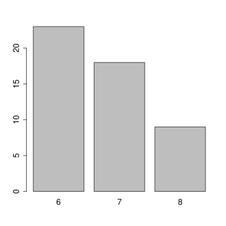
(a) DPM-CMC

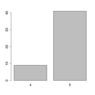
(b) DPM-MCMC

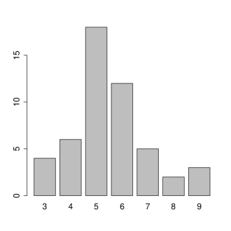
(c) FA-CMC

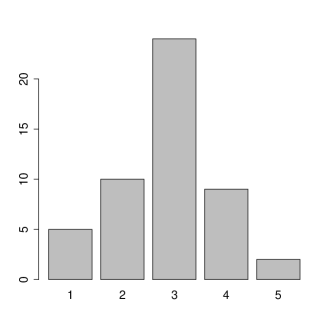
(d) FA-MCMC

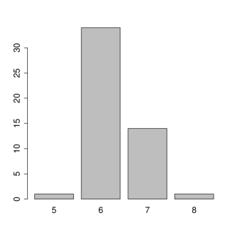
(e) DFA-CMC

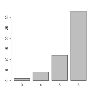
(f) DFA-MCMC

Figure 2: Simulations 1, 2 and 3: Bar plots of posterior mode $\widehat{K}$ across repeat simulations for CMC and full MCMC implementations for Simulations 1 (a and b), 2 (c and d), and 3 (e and f), respectively.

Table 1: Simulations 1, 2 and 3. We report the performance of CMC versus full MCMC for three models, DPM, FA and DFA. The error $e_{\bm{A}}$ reports the misallocation rate in estimating $\bm{A}$, and $e_{\theta}$ reports the MSE or average Hamming distance in estimating subset-specific continuous parameters (simulations 1 and 2) or categorical matrix parameters (simulation 3). The standard deviations are given within the parentheses. Both, mean and standard deviation, are with respect to repeat simulations.

	DPM			FA			DFA
	CMC	MCMC		CMC	MCMC		CMC	MCMC
$e_{\bm{A}}$	0.06 (0.03)	0.03 (0.01)		0.15 (0.05)	0.05 (0.06)		0.08 (0.01)	0.02 (0.00)
$e_{\theta}$	0.00 (0.00)	0.00 (0.00)		0.01 (0.01)	0.02 (0.03)		0.05 (0.04)	0.01 (0.01)

4.2 Simulation 2: Feature allocation using the IBP

Here, we test the performance of CMC for the FA model in Section 2.2. We generate a data matrix with $n=800$ SNVs and $p=5$ tumors. We use the same simulation truth as in Xu et al., (2015). We assume $K=4$ subclones. The latent binary matrix $\bm{A}$ is set as follows: $A_{i1}=1$ for $i=1,\dots,100$, $A_{i2}=1$ for $i=1,\dots,250$, $A_{i3}=1$ for $i=1,\dots,400$ and $A_{i4}=1$ for $i=1,\dots,600$. We draw $(b_{j},\theta^{\star}_{j1},\ldots,\theta^{\star}_{jK})\sim Dir(0.2,\bm{\pi})$ where $\bm{\pi}$ is a random permutation of $(1,5,6,10)$. We set $p_{0}=0.01$ and $N_{ij}=50$, and generate $y_{ij}$ from model (3). The same tempering scheme as in Ni et al., 2019b is adopted.

Figures 2(c) and 2(d) show the bar plots of the posterior mode $\widehat{K}$ of the number of features across simulations, under the CMC (panel (c)) and full MCMC (d) implementations. Similarly to DPM clustering, CMC tends to slightly overestimate the number of features compared to MCMC. Let $\mathcal{H}(\cdot,\cdot)$ denote the Hamming distance of two matrices and let $\#(\cdot)$ denote the total number of elements in a matrix. We define a mis-allocation rate for $\bm{A}$ as the average Hamming distance between the estimator and the truth: $e_{\bm{A}}=\frac{\mathcal{H}(\widehat{\bm{A}},\bm{A})}{\#(\bm{A})}$. In the case where $\widehat{\bm{A}}$ has more columns than $\bm{A}$, we remove the extra columns from $\widehat{\bm{A}}$. The error rate $\pi_{\theta}$ that is reported in Table 1 for the FA model summarizes the MSE in estimating the proportions $\bm{\theta}_{k}^{\star}$.

4.3 Simulation 3: Double feature allocation using an IBP prior

This simulation considers a CMC approximation of posterior inference in a DFA model with IBP prior. We generate the feature allocation matrix $\bm{A}$ from an IBP($m$) model with $m=1$ and sample size $n=1000$. The resulting matrix $\bm{A}$ has $K=6$ columns and $n=1000$ rows. Given $K=6$, we set the feature-specific parameters, $\bm{C}\in\{-1,0,1\}^{p\times K}$ with $p=60$. The heatmaps of $\bm{A}$ and $\bm{B}$ are shown in Figure S1(b)&(c), in the Supplementary Materials. The observations $y_{ij}$ are then generated from the sampling model (6).

Figures 2(e) and 2(f) show the bar plots of posterior modes $\widehat{K}$ for the number of features, across simulations for CMC (e) and full MCMC (f) implementations, respectively. As before, CMC tends to slightly overestimate the number of features compared to MCMC. The error rate $\pi_{\theta}$ that is reported in Table 1 for the DFA model summarizes the error in estimating the matched column subsets, i.e., the rows of $\bm{C}$. We use the same definition based on the Hamming distance as for $e_{\bm{A}}$.

We conclude that the proposed CMC algorithm implements a useful approximation for posterior inference on random subsets under widely used BNP models, for problems similar to the simulation scenarios, which were chosen to mimic the main features of the three motivating examples.

5 Applications

5.1 MNIST image clustering

MNIST (LeCun et al., 1998, http://yann.lecun.com/exdb/mnist/) is a dataset of images for classification, containing $n=70,000$ handwritten digits from different writers. The data is often used as a benchmark problem for clustering and classification algorithms. Each image has 28$\times$28 pixels that take values between 0 and 255 representing the grey levels. A subset of the images are shown in Figures 3(a). We visualize the high-dimensional image data with a 2D scatter plot in Figure S2 (Supplementary Materials) by using the t-distributed stochastic neighbor embedding (t-SNE, Maaten and Hinton, 2008) with perplexity parameter 75. The t-SNE algorithm is a non-linear dimension reduction tool that maps high-dimensional data onto a two- or three-dimensional manifold.

We randomly split the 70,000 images evenly into 140 shards, each with 500 images, and use one shard as anchor points. We apply the proposed CMC to the t-SNE transformed data with 5,000 iterations (discarding the first 2,500 samples and then thinning out by 5) and $\epsilon=0.1$. CMC takes less than $10$ minutes to run, whereas full MCMC simulation takes approximately 30 minutes for only the first 10 iterations. The posterior distribution of the number $K$ of clusters is shown in Figure 3(b) which is peaked at a mode at $\widehat{K}=32$. Conditional on $\widehat{K}$, the estimated clusters are depicted in Figure S2 in the Supplementary Materials. Keeping in mind that the DP prior favors many singleton clusters, we drop clusters with fewer than 1% of the total number of images (9 posterior estimated clusters were singletons), leaving 12 practically relevant clusters, which only slightly overestimates the desired number of 10 clusters. Next, we evaluate the clustering performance, relative to the known truth in this example, by computing the normalized mutual information (NMI) between the estimated partition and the true partition (induced from the true labels). Let $\bm{F}=\{F_{k}\}_{k=1}^{K}$ and $\bm{F}^{\prime}=\{F_{k^{\prime}}^{\prime}\}_{k^{\prime}=1}^{K^{\prime}}$ denote two partitions of $[n]$ and let $|F|$ denote the cardinality of a set $F$. NMI is defined as $\frac{2\times I(\bm{F};\bm{F}^{\prime})}{H(\bm{F})+H(\bm{F}^{\prime})}$, where $I(\cdot,\cdot)=\sum_{k}\sum_{k^{\prime}}\frac{|F_{k}\cap F_{k^{\prime}}^{\prime}|}{n}\log\frac{n|F_{k}\cap F_{k^{\prime}}^{\prime}|}{|F_{k}||F_{k^{\prime}}^{\prime}|}$ denotes the mutual information between two partitions $\bm{F}$ and $\bm{F}^{\prime}$ and $H(\bm{F})=-\sum_{k}\frac{|F_{k}|}{n}\log\frac{|F_{k}|}{n}$ is the entropy. NMI is between 0 and 1 with 1 being perfect match between two clusterings. NMI for CMC is 0.76 better than that of K-means 0.72 with $K=32$. Note that the purpose of this application using MNIST data is not to train a classifier or supervised model for the prediction of the 10 digits. Instead, we use the MNIST to examine the feasibility and performance of the proposed CMC algorithm for the clustering (i.e., unsupervised learning) of the relatively large dataset.

To assess the level of approximation of CMC, we use the diagnostic proposed earlier. Specifically, we sample two shards and then run CMC (using the same anchor points as before) as well as full MCMC posterior simulation on the merged dataset of the two selected shards and anchor points. Repeating the same procedure 69 times, we find an average NMI (between the estimated partitions from CMC and MCMC) of 0.85 with a standard deviation 0.02, which suggests a good approximation. We use NMI rather than more intuitive measures such as misclassification rate to account for the different numbers of clusters under CMC and MCMC. As a reference, the NMI is approximately 0.85 when we permute about 7% cluster assignments of an estimated partition from MCMC.

Sensitivity to $\epsilon$. To assess the sensitivity of the choice of $\epsilon$, we repeat the same diagnostic procedure for $\epsilon=0.05$ and $\epsilon=0.15$. The average NMI is 0.84 for both $\epsilon$’s.

Sensitivity to data split. We repeat the same analysis five times, each time with a different random split of the data. We find the results are stable, e.g. the standard deviation of the NMI (between the estimated partition and the true partition) is $<0.02$.

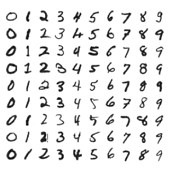
(a) MNIST handwritten digits

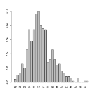
(b) Posterior distribution on $K$

Figure 3: MNIST. (a) A subset of 100 MNIST handwritten digits. (b) The posterior distribution of $K$ with mode $\widehat{K}=32$.

5.2 Inter-tumor Tumor heterogeneity

Tumors are genetically heterogeneous, often containing diverse subclones characterized by genotypic differences. Next-generation sequencing of tumor samples generates short reads from the genomes of multiple cells. Since the sequencing is performed in bulk, it is challenging to reconstruct subclones based on aggregated variant counts $y_{ij}$ (recall the notation from model (3)). FA models have been proposed in the literature to infer tumor heterogeneity, including Bayesian approaches in Lee et al., (2015) and Ni et al., 2019b . Due to the computational limitation of MCMC simulation, these methods are restricted to a relatively small number of variants (typically, $n<500$). Xu et al., (2015) proposed a scalable optimization-based algorithm (MAD-Bayes algorithm) to find a posterior mode. We will compare the proposed CMC with MAD-Bayes. We use the same pancreatic ductal adenocarcinoma (PDAC) mutation data analyzed in Xu et al., (2015). The PDAC data record the total read counts $N_{ij}$ and variant read counts $y_{ij}$ at $n=6,599$ SNVs from $p=5$ tumors.

We randomly split the 6,599 SNV’s into 33 shards. The first 32 shards have 200 SNVs each and the last shard has 199 SNVs which are used as anchor points. We apply the proposed CMC with 5,000 iterations (discarding the first 2,500 as burn-in and then thinning by 5) and the same $\epsilon=0.1$ as before. CMC takes approximately 90 minutes, whereas the full MCMC is infeasible. We find 15 major subclones across tumors after removing latent features with fewer than 5% SNVs. The estimated feature allocation matrix $\widehat{\bm{A}}$ is shown as a heatmap at the top of Figure 4. The estimated subclone proportions $\theta_{tk}^{\star}$ in each tumor are shown as a heatmap at the bottom of Figure 4. The number of subclones and the “checkerboard” pattern of the proportions suggest strong inter-tumor heterogeneity in this data.

We compare the computational efficiency with MAD-Bayes, an optimization-based approach. Since each run of MAD-Bayes algorithm may return different outputs, it is recommended to run the algorithm repeatedly (Xu et al., , 2015) (e.g. 1,000 times). MAD-Bayes has a regularization parameter $\lambda^{2}$ that controls the number $K$ of subclones. The parameter $\lambda^{2}$ needs to be carefully tuned over a range of values (say, 30 values). Using the same computer resources as for CMC (i.e. 32 computing cores), it takes more than one day to finish.

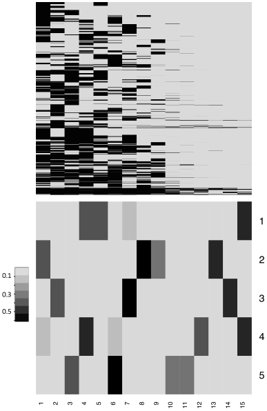
Figure 4: Tumor heterogeneity. The top part of the heatmap shows the estimated subclonal genotypes $\bm{A}$ of the selected SNV with dark and light cells representing 1 (mutant) and 0 (wildtype), respectively. The columns are subclones and the rows are SNVs. The bottom part of the heatmap shows the estimated proportions $\theta_{tk}^{\star}$ of subclones in each tumor. The columns are subclones and the rows are tumors.

5.3 Electronic health records phenotyping

We consider a large EHR dataset with $n=100,000$ patients from China. The data are from a physical exam of Chinese residents in 2016. We extract the blood test results measured on $p=39$ testing items (shown in Table 2) and diagnostic codes for diabetes from the EHR. We implement inference under a DFA prior and sampling model (6). Each latent feature can be interpreted as a latent disease that favors symptoms $R_{k}=\{j\mid C_{jk}=1\}$ and is related to a subset of patients $F_{k}=\{i\mid A_{ik}=1\}$. That is, $\bm{A}$ describes the patient-disease relationships and $\bm{C}$ describes symptom-disease relationships. We follow the same procedure in Ni et al., (2019) to preprocess the data. Using the reference range for each test item, we discretize the data and define a symptom if the value of an item falls beyond the reference range. We fix the first column of $\bm{A}$ in the DFA model according to the diabetes diagnosis. Moreover, since diabetes is clinically associated with high glucose level, we incorporate this prior information by fixing the corresponding entry in the first column of $\bm{C}$. Additional prior knowledge regarding the symptom-disease relationships is incorporated. Creatinine and blood urea nitrogen (BUN) are two important indicators of kidney disease. High levels of these two items suggest impaired kidney function. We fix the two entries (corresponding to creatinine and BUN) of the second column of $\bm{C}$ to 1 and the rest to 0. Similarly, elevated systolic blood pressure and diastolic blood pressure indicate hypertension, and abnormal levels of total bilirubin (TB), aspartate aminotransferase (AST) and alanine aminotransferase (ALT) are indicators of liver diseases. We fix the corresponding entries of the third and fourth column of $\bm{C}$.

We randomly split the 100,000 patients evenly into 500 shards, each with 200 patients, and use one shard as anchor points. We apply the proposed CMC with 50,000 iterations (discarding the first 25,000 as burn-in and then thinning out to every 10th) and the same $\epsilon=0.1$ as before. CMC simulation takes approximately 1 hour, whereas full MCMC takes 90 minutes for the first 10 iterations. We find 8 major latent diseases in addition to the 4 known diseases after removing tiny latent features (with $<$1% patients). The estimated symptom-disease relationships $\widehat{\bm{C}}$ are represented by a bipartite network in Figure 5 and also as a heatmap in Figure S3 (Supplementary Materials). The estimated patient-disease relationships $\widehat{\bm{A}}$ for 1000 randomly selected patients are shown as a heatmap in Figure S3.

Unlike MNIST or the application to tumor heterogeneity, there is no ground truth or alternative implementation for posterior inference for the full data. Instead we compare the results with previous results by Ni et al., (2019) who used a full MCMC implementation for a subset of 1000 patients from the same dataset. Some of our findings are consistent with the earlier results, which suggests a good approximation of the proposed CMC to full MCMC. Moreover, with a hundred times more observations, we are able to find more interpretable results compared to theirs.

Latent disease X1 (previously referred to as lipid disorder) is primarily associated with elevated total cholesterol (TC) and low density lipoprotein (LDL). Patients with high levels of TC and LDL have higher risks of heart disease and stroke. Latent diseases X2 and X3 are associated with the same set of symptoms but with opposite signs. This interesting result is also found in Ni et al., (2019) where X2 and X3 were identified as polycythemia and anemia, respectively. Each of X5, X6 and X8 also finds good correspondence in Ni et al., (2019) as bacterial infection, viral infection and thrombocytopenia.

One prevelant latent disease reported in Ni et al., (2019) does not have a clear interpretation due to the excessive number of symptoms. They suspect a subset of symptoms like decreased plateletcrit (PCT), leukocytes and GRA are due to weak immune system of the elderly population. However, other symptoms are not related to immune system. With a much larger sample size, we are able to single out those symptoms without spurious links through the latent disease X7.

Table 2: Blood test items. Acronyms are given within parentheses. CV indicates coefficient of variation, “dist” is distribution, “mn” is mean, “ct”is count, and “conc” is concentration.

alanine aminotransferase (ALT)	aspartate aminotransferase (AST)	total bilirubin (TB)
total cholesterol (TC)	triglycerides	low density lipoproteins (LDL)
high density lipoproteins (HDL)	urine pH (UrinePH)	mn corpuscular hemoglobin conc (MCHC)
% of monocytes (%MON)	alpha fetoprotein (AFP)	carcinoembryonic antigen (CEA)
number of monocytes (#MON)	plateletcrit (PCT)	CV of platelet dist. (PDW-CV)
% of eosinophil (%Eosinophil)	basophil ct (#Basophil)	% of basophil (%Basophil)
platelet large cell ratio (P-LCR)	platelets	systolic blood pressure (Systolic)
% of granulocyte (%GRA)	body temperature (BodyTemperature)	leukocytes
hemoglobin	creatinine	blood urea nitrogen (BUN)
glucose	diastolic blood pressure (Diastolic)	heart rate (HeartRate)
erythrocytes	hematocrit (HCT)	uric acid (UricAcid)
% of lymphocyte (%LYM)	mn corpuscular volume (MCV)	mn corpuscular hemoglobin (MCH)
lymphocyte ct (#LYM)	granulocyte ct (#GRA)	mn platelet volume (MPV)

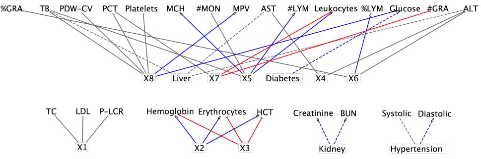
Figure 5: EHR. Bipartite network for symptom-disease relationships from DFA. The diseases are represented by rectangles. Latent diseases are represented by X1$,\dots,$X8. Solid lines are symptom-disease relationships inferred from the data whereas dashed lines are fixed by prior knowledge. Undirected edges indicate the symptoms are binary. Directed edges with bars (arrowheads) indicate the disease causes the symptom to be lower (higher) than normal range.

6 Discussion

We have developed a simple CMC algorithm for fast approximate posterior inference of BNP models. The proposed CMC is a general algorithm in the sense that it can be used to scale up practically any Bayesian clustering and feature allocation methods. CMC runs MCMC on subsets of observations in parallel and aggregates the Monte Carlo samples. The main idea of this paper is using a subset of observations as anchor points to merge clusters or latent features from different machines. The aggregation step has a tuning parameter $\epsilon$ which is not influential of the results in our simulations and applications. We have focused on point estimation throughout the paper. But the proposed algorithm provides an efficient approximation of the entire posterior distribution. The output of the proposed algorithm is a consensus Monte Carlo sample for the whole data posterior, which can be used for any Monte Carlo based posterior inference. For example, to find the 90% credible interval of a continuous parameter, one can take the 5% and 95% sample quantiles of the consensus Monte Carlo sample. For discrete structures such as partitions, one can use the approach in Wade et al., (2018) to construct credible balls of partitions, again using the consensus Monte Carlo sample.

The anchor points are randomly chosen. Overall, we find that inference remains robust with respect to the choice of the anchor points, as long as the number of anchor points is sufficiently large. The analysis in Section 5.1 leads to similar results (not shown) under different random splits of the data. Alternatively to using randomly chosen anchor points, one may use big-data summarization approaches to guide the choice, using for example the notion of a “coreset” developed in Huggins et al., (2016); Campbell and Broderick, (2019). Alternatively, Mak and Joseph, (2018) proposed a small set of “support points” to represent a continuous probability distribution.

We explicitly address the problem of large sample size but have not considered the issue of high-dimensionality. We discussed the approach for random subsets in random partitions and (double) feature allocation. In the motivating examples we used DPM and IBP priors. But the algorithm remains equally valid for any other prior model. The approach with common anchors remains useful also for any other models that involve random subsets that can be split and merged in a similar fashion, including latent trait models, finite mixture models, and finite feature allocation.

Supplementary Materials

Additional figures

S1 through S3 for simulations and applications. (.pdf file)

Software

to merge Monte Carlo samples of clusters and latent features and to generate all simulated data.

References

- Argiento et al., (2010) Argiento, R., Guglielmi, A., and Pievatolo, A. (2010). Bayesian density estimation and model selection using nonparametric hierarchical mixtures. Computational Statistics & Data Analysis, 54(4):816 – 832.
- Barrios et al., (2013) Barrios, E., Lijoi, A., Nieto-Barajas, L. E., and Prünster, I. (2013). Modeling with normalized random measure mixture models. Statistical Science, 28(3):313–334.
- Blei et al., (2006) Blei, D. M., Jordan, M. I., et al. (2006). Variational inference for Dirichlet process mixtures. Bayesian Analysis, 1(1):121–143.
- (4) Broderick, T., Jordan, M. I., and Pitman, J. (2013a). Cluster and feature modeling from combinatorial stochastic processes. Statistical Science, 28(3):289–312.
- (5) Broderick, T., Kulis, B., and Jordan, M. (2013b). MAD-Bayes: MAP-based asymptotic derivations from Bayes. In International Conference on Machine Learning, pages 226–234.
- (6) Broderick, T., Pitman, J., Jordan, M. I., et al. (2013c). Feature allocations, probability functions, and paintboxes. Bayesian Analysis, 8(4):801–836.
- Campbell and Broderick, (2019) Campbell, T. and Broderick, T. (2019). Automated scalable Bayesian inference via Hilbert coresets. The Journal of Machine Learning Research, 20(1):551–588.
- de Blasi et al., (2015) de Blasi, P., Favaro, S., Lijoi, A., Mena, R. H., Prünster, I., and Ruggiero, M. (2015). Are Gibbs-type priors the most natural generalization of the Dirichlet process? IEEE Transactions on Pattern Analysis and Machine Intelligence, 37:212–229.
- (9) Doshi-Velez, F., Miller, K., Van Gael, J., and Teh, Y. W. (2009a). Variational inference for the Indian buffet process. In Artificial Intelligence and Statistics, pages 137–144.
- (10) Doshi-Velez, F., Mohamed, S., Ghahramani, Z., and Knowles, D. A. (2009b). Large scale nonparametric Bayesian inference: Data parallelisation in the Indian buffet process. In Advances in Neural Information Processing Systems, pages 1294–1302.
- Entezari et al., (2018) Entezari, R., Craiu, R. V., and Rosenthal, J. S. (2018). Likelihood inflating sampling algorithm. Canadian Journal of Statistics, 46(1):147–175.
- Favaro and Teh, (2013) Favaro, S. and Teh, Y. W. (2013). MCMC for normalized random measure mixture models. Statistical Science, 28(3):335–359.
- Ge et al., (2015) Ge, H., Chen, Y., Wan, M., and Ghahramani, Z. (2015). Distributed inference for Dirichlet process mixture models. In Proceedings of the 32nd International Conference on Machine Learning, pages 2276–2284.
- Ghahramani and Griffiths, (2006) Ghahramani, Z. and Griffiths, T. L. (2006). Infinite latent feature models and the Indian buffet process. In Advances in Neural Information Processing Systems, pages 475–482.
- Ghoshal, (2010) Ghoshal, S. (2010). The Dirichlet process, related priors and posterior asymptotics. In Hjort, N. L., Holmes, C., Müller, P., and Walker, S. G., editors, Bayesian Nonparametrics, pages 22–34. Cambridge University Press.
- Hartigan, (1972) Hartigan, J. A. (1972). Direct clustering of a data matrix. Journal of the American Statistical Association, 67(337):123–129.
- Huang and Gelman, (2005) Huang, Z. and Gelman, A. (2005). Sampling for Bayesian computation with large datasets. Technical report, Department of Statistics, Columbia University.
- Huggins et al., (2016) Huggins, J., Campbell, T., and Broderick, T. (2016). Coresets for scalable Bayesian logistic regression. In Advances in Neural Information Processing Systems, pages 4080–4088.
- Kingman, (1978) Kingman, J. F. C. (1978). The representation of partition structures. J. London Math. Soc. (2), 18(2):374–380.
- Kunkel and Peruggia, (2018) Kunkel, D. and Peruggia, M. (2018). Anchored bayesian gaussian mixture models. arXiv preprint arXiv:1805.08304.
- Kurihara et al., (2007) Kurihara, K., Welling, M., and Teh, Y. W. (2007). Collapsed variational Dirichlet process mixture models. In IJCAI, volume 7, pages 2796–2801.
- Lau and Green, (2007) Lau, J. W. and Green, P. J. (2007). Bayesian model-based clustering procedures. Journal of Computational and Graphical Statistics, 16(3):526–558.
- LeCun et al., (1998) LeCun, Y., Bottou, L., Bengio, Y., Haffner, P., et al. (1998). Gradient-based learning applied to document recognition. Proceedings of the IEEE, 86(11):2278–2324.
- Lee et al., (2015) Lee, J., Müller, P., Gulukota, K., and Ji, Y. (2015). A Bayesian feature allocation model for tumor heterogeneity. Ann. Appl. Stat., 9(2):621–639.
- Lijoi et al., (2005) Lijoi, A., Mena, R. H., and Prünster, I. (2005). Hierarchical mixture modeling with normalized inverse-Gaussian priors. Journal of the American Statistical Association, 100(472):1278–1291.
- Lijoi et al., (2007) Lijoi, A., Mena, R. H., and Prünster, I. (2007). Controlling the reinforcement in Bayesian non-parametric mixture models. Journal of the Royal Statistical Society: Series B, 69(4):715–740.
- Lin, (2013) Lin, D. (2013). Online learning of nonparametric mixture models via sequential variational approximation. In Advances in Neural Information Processing Systems, pages 395–403.
- Lo, (1984) Lo, A. Y. (1984). On a class of Bayesian nonparametric estimates: I. Density estimates. The Annals of Statistics, 12(1):351–357.
- Maaten and Hinton, (2008) Maaten, L. v. d. and Hinton, G. (2008). Visualizing data using t-sne. Journal of Machine Learning Research, 9(Nov):2579–2605.
- MacEachern, (2000) MacEachern, S. N. (2000). Dependent Dirichlet processes. Unpublished manuscript, Department of Statistics, The Ohio State University, pages 1–40.
- Mak and Joseph, (2018) Mak, S. and Joseph, V. R. (2018). Support points. The Annals of Statistics, 46(6A):2562–2592.
- Minsker et al., (2014) Minsker, S., Srivastava, S., Lin, L., and Dunson, D. (2014). Scalable and robust Bayesian inference via the median posterior. In International Conference on Machine Learning, pages 1656–1664.
- Neal, (2000) Neal, R. M. (2000). Markov chain sampling methods for dirichlet process mixture models. Journal of Computational and Graphical Statistics, 9(2):249–265.
- Neiswanger et al., (2013) Neiswanger, W., Wang, C., and Xing, E. (2013). Asymptotically exact, embarrassingly parallel MCMC. arXiv preprint arXiv:1311.4780.
- Newton et al., (1998) Newton, M. A., Quintana, F. A., and Zhang, Y. (1998). Nonparametric Bayes methods using predictive updating. In Practical nonparametric and semiparametric Bayesian statistics, pages 45–61. Springer.
- Ni et al., (2019) Ni, Y., Mueller, P., and Ji, Y. (2019). Bayesian Double Feature Allocation for Phenotyping with Electronic Health Records. Journal of the American Statistical Association, page in press.
- (37) Ni, Y., Müller, P., Diesendruck, M., Williamson, S., Zhu, Y., and Ji, Y. (2019a). Scalable bayesian nonparametric clustering and classification. Journal of Computational and Graphical Statistics, page in press.
- (38) Ni, Y., Müller, P., Shpak, M., and Ji, Y. (2019b). Parallel-Tempered Feature Allocation for Large-scale Tumor Heterogeneity with Deep Sequencing Data. Technical Report.
- Pitman and Yor, (1997) Pitman, J. and Yor, M. (1997). The two-parameter Poisson-Dirichlet distribution derived from a stable subordinator. The Annals of Probability, pages 855–900.
- Rabinovich et al., (2015) Rabinovich, M., Angelino, E., and Jordan, M. I. (2015). Variational consensus Monte Carlo. In Advances in Neural Information Processing Systems, pages 1207–1215.
- Rai and Daume, (2011) Rai, P. and Daume, H. (2011). Beam search based map estimates for the Indian buffet process. In Proceedings of the 28th International Conference on Machine Learning (ICML-11), pages 705–712. Citeseer.
- Reed and Ghahramani, (2013) Reed, C. and Ghahramani, Z. (2013). Scaling the Indian buffet process via submodular maximization. In International Conference on Machine Learning, pages 1013–1021.
- Richardson and Green, (1997) Richardson, S. and Green, P. J. (1997). On Bayesian analysis of mixtures with an unknown number of components (with discussion). Journal of the Royal Statistical Society: series B, 59(4):731–792.
- Rodriguez et al., (2011) Rodriguez, A., Lenkoski, A., and Dobra, A. (2011). Sparse covariance estimation in heterogeneous samples. Electronic Journal of Statistics, 5:981.
- Scott et al., (2016) Scott, S. L., Blocker, A. W., Bonassi, F. V., Chipman, H. A., George, E. I., and McCulloch, R. E. (2016). Bayes and big data: The consensus Monte Carlo algorithm. International Journal of Management Science and Engineering Management, 11(2):78–88.
- Tank et al., (2015) Tank, A., Foti, N., and Fox, E. (2015). Streaming variational inference for Bayesian nonparametric mixture models. In Proceedings of the Eighteenth International Conference on Artificial Intelligence and Statistics, pages 968–976.
- Wade et al., (2018) Wade, S., Ghahramani, Z., et al. (2018). Bayesian cluster analysis: Point estimation and credible balls (with discussion). Bayesian Analysis, 13(2):559–626.
- Wang and Dunson, (2011) Wang, L. and Dunson, D. B. (2011). Fast Bayesian inference in Dirichlet process mixture models. Journal of Computational and Graphical Statistics, 20(1):196–216.
- Wang and Dunson, (2013) Wang, X. and Dunson, D. B. (2013). Parallelizing MCMC via Weierstrass sampler. arXiv preprint arXiv:1312.4605.
- White et al., (2015) White, S., Kypraios, T., and Preston, S. (2015). Piecewise Approximate Bayesian Computation: fast inference for discretely observed Markov models using a factorised posterior distribution. Statistics and Computing, 25(2):289.
- Williamson et al., (2013) Williamson, S. A., Dubey, A., and Xing, E. P. (2013). Parallel Markov chain Monte Carlo for nonparametric mixture models. In Proceedings of the 30th International Conference on International Conference on Machine Learning, pages 98–106.
- Xu et al., (2015) Xu, Y., Müller, P., Yuan, Y., Gulukota, K., and Ji, Y. (2015). MAD Bayes for tumor heterogeneity – feature allocation with exponential family sampling. Journal of the American Statistical Association, 110(510):503–514.
- Zuanetti et al., (2019) Zuanetti, D. A., Müller, P., Zhu, Y., Yang, S., and Ji, Y. (2019). Bayesian nonparametric clustering for large data sets. Statistics and Computing, 29:203–215.