Peak Age of Information in Priority Queueing Systems

Abstract

We consider a priority queueing system where a single processor serves $k$ classes of packets that are generated randomly following Poisson processes. Our objective is to compute the expected Peak Age of Information (PAoI) under various scenarios. In particular, we consider two situations where the buffer size at each queue is one and infinite, and in the infinite buffer size case we consider First Come First Serve (FCFS) and Last Come First Serve (LCFS) as service disciplines. For the system with buffer size one at each queue, we derive PAoI exactly for the case of exponential service time and bounds (which are excellent approximations) for the case of general service time, with small $k$. For the system with infinite buffer size, we provide closed-form expressions of PAoI for both FCFS and LCFS where service time is general and $k$ could be large. Using those results we investigated the effect of ordering of priorities and service disciplines for the various scenarios. We perform extensive numerical studies to validate our results and develop insights.

I Introduction

In the recent years, the notion of Age of Information (AoI) has garnered attention from many researchers. The main applications that have been cited include sensor networks, wireless networks, and autonomous vehicle systems [1], as it is important to know the freshness of information in all those cases. Our research has been motivated by an application in smart manufacturing where edge devices, sensors in particular, with limited processing capabilities, would monitor the health of various tools, condition of components, and quality of work pieces in machines. This sensed information would be used for timely decisions such as tool changes, re-calibration and rework, thereby improving overall quality of the manufactured products. In such a scenario, decisions may be made based on delayed information due to the discontinuous sampling and long information processing time. Hence it is crucial to consider the freshness of information in decision making, for some type of which AoI is an ideal choice.

AoI is a metric defined and used by researchers such as Kaul et al [1] to describe the freshness of data. We consider a system where a data source (sensor or resource) from time to time sends updates or files (in this paper we call each update or file a “packet”) to the processor (also called server). The time when a packet is generated by a data source is called its arrival time (also called release time) into the system. The server processes packets in a non-preemptive way. Unprocessed packets are queued due to the limited processing capacity of the server. AoI at an arbitrary time point $t$ is defined as the length of period between time $t$ and the most recent release time among all the packets that have been processed. Mathematically, the AoI at time $t$ is defined as $\triangle(t)=t-\max\{r_{l}:C_{l}\leq t\}$, where $r_{l}$ is the release time of the $l^{th}$ packet that is generated and $C_{l}$ is the time when it is processed by the server (also called its completion time). While the time-average AoI could be a metric to measure data freshness, many researchers consider Peak Age of Information (PAoI) as a more tractable metric [2, 3]. We let the $n^{th}$ peak value of $\triangle(t)$ be $A_{n}$, which is a random variable and it is shown in Figure 1. By assuming ergodicity, the limit expectation of this peak value, i.e., $\boldsymbol{E}[A]=\lim_{n\rightarrow\infty}\boldsymbol{E}[A_{n}]$, is then defined as PAoI for this data source. We will later extend this notion to multiple sources and formulate our model.

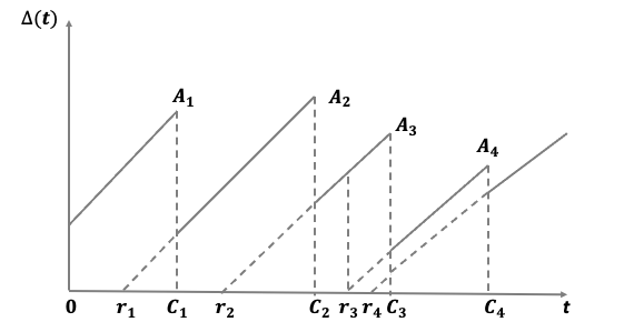
Figure 1: Age of Information for a Single Queue

It has been well documented and accepted that monitoring and sensing according to a Poisson process is effective [4]. In that light we consider multiple data sources (sensors) that monitor according to a Poisson process with potentially different rates due to the difficulty in sensing (recall our motivation example of a manufacturing setting). We consider a setting where there are $k$ data sources prioritized from 1 (highest) to $k$ (lowest). There is a single server that “serves” the $k$ packet streams based on a static priority mechanism. We study the static queue priorities mainly because in many cases, there are some data sources whose packets contain age sensitive information or emergency information such as high temperature, high pressure (see [5]). These data packets need to be transmitted as soon as possible, thus high static priorities for these data sources are needed. Another example is given by Maatouk et al [6], which says that in the vehicle network, the safety related data should be allocated higher priorities over the other non-safety related data to improve the traveling experience. All these real applications motivate us to consider a multi-queue system with static priorities.

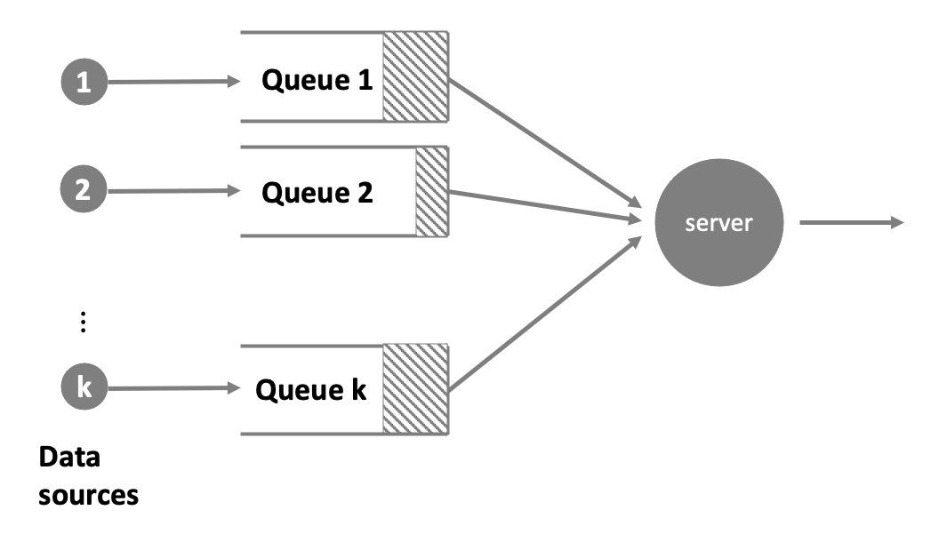
Figure 2: System Model

The system model is provided in Figure 2. We consider two settings in this paper: one in which there is a buffer at each queue that can hold at most one packet at a time; the other where each buffer can hold infinitely many packets. For the first setting we discuss the system M/G/1/1$+\sum 1^{*}$ and M/G/1/1$+\sum 1$ for general service times. The notation $1+\sum 1^{*}$ means besides the processing area at the server, each data source has a buffer with size one. The asterisk means that the packet waiting in the buffer is replaced by the newest arrival, the same as the notation used in [7, 8]. If there is no asterisk, i.e., M/G/1/1$+\sum 1$, then it means that packet that enters the buffer will not be replaced by new arrivals. For the setting of infinite buffer size, we discuss the M/G/1 type queues with First Come First Serve (FCFS) and Last Come First Serve (LCFS) service disciplines respectively. It is still unknown which setting and which discipline will result in the smallest PAoI. So our objective is to derive the PAoI for each setting, and then find the optimal setting and discipline. The main contributions of our paper are listed as follows:

1. We first provide a novel modeling method to evaluate PAoI of multi-queue systems by focusing on the busy period of server and buffer status. Using this method we provide the exact PAoI for the prioritized system M/M/1/$1+\sum 1^{*}$ and system M/G/1/$1+\sum 1$ with small number of queues $k$. And we further provide the bounds (which are also excellent approximations) for PAoI of the system M/G/1/$1+\sum 1^{*}$.

2. We provide the exact PAoI for the infinite buffer prioritized system M/G/1 with FCFS and LCFS for general number of queues $k$, and our analysis for deriving PAoI under LCFS can be applied to other systems with LCFS as well.

3. By providing the exact PAoI of systems above, we show a surprising result that LCFS is not the optimal service discipline for minimizing PAoI among all the non-preemptive work-conserving disciplines in the system where buffer size of each queue is infinite. We also show a counter-intuitive finding that having a single buffer at each queue does not always provide lower PAoI than the having a buffer with infinite size. We further reveal that it is because the special definition of the metric PAoI.

4. We reveal the fact that PAoI of queues with low priorities are sensitive to the traffic intensity of queues with high priorities, so queues that contain important or time-sensitive information should be given high priorities. Also, if the PAoI averaged across queues is to be minimized, we show that it is beneficial to assign low priorities to high traffic queues.

The rest of this paper is organized as follows. A summary of the literature is provided in Section II. Then, in Section III we provide the PAoI analysis for M/G/1/1+$\sum 1^{*}$ and M/G/1/1$+\sum 1$ type queues. In Section IV we provide the PAoI analysis for queues with infinite buffer size, under both FCFS and LCFS disciplines within each queue. We perform numerical studies in Section V, and make concluding remarks as well as discuss the future work in Section VI.

II Related Work

The idea of data age, information freshness, and timeliness for data warehouses are introduced and discussed in [9, 10]. In recent years, data freshness has drawn much more attention because of the development of Internet of Things, fog computing and edge data storage [11, 12]. Kaul et al [1] firstly provided average AoI for M/M/1, M/D/1 and D/M/1 type queues. Costa et al [7] then obtained analytical results of average AoI and PAoI under FCFS for M/M/1/1, M/M/1/2 (which allows drop of new arrivals), as well as M/M/1/2* (which allows update for the waiting packet) queues. The performance of LCFS policy for the single buffer case where service times are gamma distributed was provided by Najm and Nasser [13]. Soysal and Ulukus [14] considered G/G/1/1 type queues and provided bounds of AoI for different arrival and service processes. Zou et al [8] discussed PAoI and AoI under the waiting procedure in M/G/1/1 and M/G/1/2* cases. Kosta et al [15] discussed the performance of AoI and PAoI for the single-queue slotted-time system with and without packets management. Inoue et al [3] discussed the relationship between PAoI and AoI for the single queue case, and they provided the AoI/PAoI analysis for different single queue models including M/G/1 and G/M/1 systems with FCFS, preemptive LCFS, and non-preemptive LCFS. Some recent works have considered AoI for the system with single server and multiple queues. Huang and Modiano [2] provided the PAoI for multi-class M/G/1 and M/G/1/1 queues where all packets flow into a combined queue. Najm and Telatar [16] considered the M/G/1/1 system with multiple sources updating while allowing preemption. Kosta et al [17] considered a slotted-time system and discussed the performance of round-robin, working-conserving and random policy. Jiang et al [18] considered an AoI minimization problem with Bernoulli arrivals in a slotted-time system and modeled it as a MDP problem to determine which data source to serve next. They showed that Whittle’s index policy is a near optimal policy and they also provided a decentralized policy which achieves nearly identical performance as the Whittle’s index policy. The optimality of Whittle’s index policy was further discussed by Maatouk et al in [19]. Kadota et al [20] considered an AoI minimization problem in a slotted-time system with throughput constraint considerations. Talak et al [21] considered weighted AoI and PAoI minimization problem in a discrete timed system with channel errors. It is also pointed out by [21] that the PAoI/AoI for the discrete time queues may differ significantly from their continuous time counterpart. Other AoI/PAoI minimization problems for discrete time systems can be found in [22, 23, 18, 24, 25, 26]. The multi-class queues with FCFS and LCFS across queues are discussed in Yates and Kaul [27]. A detailed review for the current literature for AoI was also provided in [27].

However, we notice that if all the packets arriving into the multi-queue system are served following FCFS or LCFS regardless of their classes (queues), queues with high arrival rates will be served more frequently. It is not always the case that the queues with high arrival rates are important. Queues with low traffic intensities may also be important, and their packets may need to be processed as soon as the server becomes available. Besides, spending too much time processing a certain data source is a waste of service resource. We thus want to consider a service policy which gives certain queues higher priorities. Such a multiple-queue system with queue priorities has been studied for a long time, however most of previous works focused on different metrics such as queue lengths and waiting time distributions [28, 29]. AoI and PAoI are metrics introduced in recent years, and their performance under queue priorities are not well understood. Najm et al [5] considered a system with two streams of different priorities and discussed different service disciplines for the low priority stream. Recently, Kaul and Yates [30] modeled the AoI of M/M/1 priority queues as a hybrid system by assuming the waiting room (buffer size) for the system is either null or one. However, their model is restrictive since there is at most one buffer for all queues. Maatouk et al [6] discussed the model where each queue has an individual buffer, and provided a closed-form expression for AoI using a hybrid system analysis. However, it is assumed in [6] that arrival and service rates for all queues are exponential and identical. It is still unknown if having finite buffer can help reduce PAoI for each queue in the multi-queue scenario, especially when arrival and service rates differ from one queue to another. In our work, we for the first time provide the exact PAoI for the system where queues are prioritized and each queue has its own waiting room (buffer), arrival rate, and service rate. In this paper we only consider static queue priorities because in many applications, some data streams have more important information which need to be transmitted as soon as possible. Moreover, the queue performance is more tractable when queue priorities are fixed, but the behavior of PAoI in this case is still not fully understood. In this paper, we provide a new modeling approach of calculating PAoI by focusing on the buffer status. We derive the exact PAoI for M/M/$1+\sum 1^{*}$ system and M/G/$1+\sum 1$ system, as well as bounds for M/G/$1+\sum 1^{*}$ queues with priorities. Also, for the case of infinite buffer size, we derive the exact PAoI for M/G/1 system with FCFS and LCFS service disciplines within each queue. We seek to find a priority order and service discipline that would result in low average PAoI across queues. We also seek to understand the effect of arrival rates and service times on the PAoI for systems under different settings for buffer size and service disciplines.

III Queues with Buffer Size One

In this section we discuss the system M/G/1/1+$\sum 1^{*}$ with the arrival process for each queue $i$ being a Poisson process with rate $\lambda_{i}$. The service time (processing time) $P_{i}$ for packets from queue $i$ is an i.i.d. random variable with cdf $F_{i}(x)$ and mean $\frac{1}{\mu_{i}}.$ A new arrival will replace the packet waiting in the queue (if there is one) since the newest packet contains the most recent information of the source. Note that this model is different from the M/G/1/1 model introduced in [2, 16]. In their model, there is no buffer for each queue, so whenever a packet arrives and sees the server being busy, the packet is either rejected or preempts the packet in service. In our model, the assumption of buffer at each queue allows the server to serve queues in a prioritized way. Moreover, keeping only the most recent packet in the buffer can reduce the server’s load, and also guarantee that the freshest information is stored in the buffer.

The difficulty in analyzing such a system with buffer at each queue is that packets served by the server are only a subset of packets generated by the data source, due to some getting replaced. Focusing on how each packet goes through the system often makes modeling more complicated [30]. Instead, in this paper we introduce a new modeling approach to derive PAoI, which is to incorporate the buffer state. We can also use this idea to derive PAoI for other systems with buffer size more than one, as we will see in Section IV. We depict a sample path of the buffer state for queue $i$ in Figure 3 with notations described subsequently. From Figure 3 we can see that buffer state of queue $i$ is either $0$ or $1$. When the buffer state is 1 (the buffer is full), we say the buffer is busy. We use $r_{ij}$, $S_{ij}$ and $C_{ij}$ to denote the release time, starting time of processing and completion time of $j^{th}$ packet that arrives at queue $i$ (note that $S_{ij}$ and $C_{ij}$ only exist if the packet is processed by the server). Suppose at time $r_{i1}$, packet $1$ arrives at queue $i$. It waits until time $S_{i1}$, when the server becomes available to serve it. Right after time $S_{i1}$, buffer $i$ keeps empty until packet 2 arrives at time $r_{i2}$. Packet $2$ stays in the buffer for a while, then gets replaced by packet $3$ at time $r_{i3}$. Packet 3 is then replaced by packet 4 at time $r_{i4}.$ At time $S_{i4}$ the server becomes available and starts serving packet 4, and the buffer becomes empty again. The service of packet 4 is completed at time $C_{i4},$ and the peak age of information upon the completion of packet 4 is given as $C_{i4}-r_{i1}$, which is equal to

$$C_{i4}-r_{i1} = (C_{i4}-S_{i4})+(S_{i4}-r_{i2})$$ (1)

$$+(r_{i2}-S_{i1})+(S_{i1}-r_{i1}).$$

The term $(C_{i4}-S_{i4})$ of Equation (1) is the processing time of packet 4, and $(S_{i4}-r_{i2})$ is the time period during which the buffer has one packet. The third term $(r_{i2}-S_{i1})$ is the time period during which the buffer stays empty, and the last term $(S_{i1}-r_{i1})$ is the waiting time of packet 1. Recall that the processing times of packets from the same source are i.i.d., so the expected value of $(C_{i4}-S_{i4})$ is $\boldsymbol{E}[P_{i}]=\frac{1}{\mu_{i}}.$ The buffer is empty during time $(r_{i2}-S_{i1})$, and from the memoryless property of exponential inter-arrival times, we know the expected length of $(r_{i2}-S_{i1})$ is $\boldsymbol{E}[I_{i}]=\frac{1}{\lambda_{i}}$. Therefore we can write the PAoI for source $i$ as

$$\boldsymbol{E}[A_{i}] = \boldsymbol{E}[P_{i}]+\boldsymbol{E}[W_{i}]+\boldsymbol{E}[I_{i}]+\boldsymbol{E}[G_{i}],$$ (2)

where $\boldsymbol{E}[G_{i}]$ is the expected waiting time (in buffer) of a packet that is eventually processed by the server, and $\boldsymbol{E}[W_{i}]$ is the expected length of time period when the buffer is continuously busy. Note that Equation (2) holds true for every queue $i$. For M/G/1/1+$sum1^{*}$ type queues, we have already stated that $\boldsymbol{E}[P_{i}]=\frac{1}{\mu_{i}}$ and $\boldsymbol{E}[I_{i}]=\frac{1}{\lambda_{i}}$. The difficult part in deriving PAoI remains in calculating $\boldsymbol{E}[W_{i}]$ and $\boldsymbol{E}[G_{i}]$. Notice that $W_{i}$ is the period that the buffer is full, and it is not determined by which packet we keep in the buffer. If we reject the new arrivals (instead of the system that we are analyzing) when the buffer is full, then $W_{i}$ is the waiting time for the packet that enters the buffer. Using this property, if we let $p_{i}$ be the probability that buffer $i$ is full, then from Little’s Law [31] we know the average queue length is $p_{i}=\lambda_{i}(1-p_{i})\boldsymbol{E}[W_{i}]$. So we have

$$\boldsymbol{E}[W_{i}] = \frac{p_{i}}{\lambda_{i}(1-p_{i})}.$$ (3)

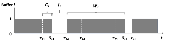
Figure 3: Buffer State for Queue $i$

From Equation (3), $\boldsymbol{E}[W_{i}]$ can be obtained once we know $p_{i}.$ We shall discuss how to find $p_{i}$ later in this section. Now we continue with the system where new arrivals replace the existing ones in buffer. We first characterize $G_{i}$, which depends on $W_{i}$, as we will see in Lemma 1.

Lemma 1.

$\boldsymbol{E}[G_{i}|W_{i}]=\frac{1}{\lambda_{i}}(1-\boldsymbol{E}[e^{-\lambda_{i}W_{i}}]).$

Proof:

Suppose $N(t)=m$ packets arrive during $W_{i}$, then $G_{i}$ is the time gap from the arrival time of the $m^{th}$ packet to time $t$. From Campbell’s Theorem (P173, Theorem 5.14 in [32]) we have for $x\leq t$,

$$\boldsymbol{P}(G_{i}<x|N(t)=m,W_{i}=t)$$

$$= \boldsymbol{P}(R_{m}>t-x|N(t)=m,W_{i}=t)$$

$$= \int_{t-x}^{t}\frac{m}{t}(\frac{u}{t})^{m-1}du$$

$$= 1-(\frac{t-x}{t})^{m}.$$

Thus by integrating $\boldsymbol{P}(G_{i}>x|N(t)=m,W_{i}=t)$ for $x$ from $0$ to $t$, we have

$$\boldsymbol{E}[G_{i}|N(t)=m,W_{i}=t]=\frac{t}{m+1}.$$

Then, unconditioning using $\boldsymbol{P}(N(t)=m)=e^{-\lambda_{i}t}\frac{(\lambda_{i}t)^{m}}{m!}$, we get

$$\boldsymbol{E}[G_{i}|W_{i}=t] = \sum_{m=0}^{\infty}\frac{t}{m+1}e^{-\lambda_{i}t}\frac{(\lambda_{i}t)^{m}}{m!}$$

$$= \sum_{m=0}^{\infty}e^{-\lambda_{i}t}\frac{(\lambda_{i}t)^{m+1}}{(m+1)!}\frac{1}{\lambda_{i}}$$

$$= \frac{e^{-\lambda_{i}t}}{\lambda_{i}}(e^{\lambda_{i}t}-1).$$

∎

Lemma 1 shows that one needs to know the Laplace–Stieltjes transform (LST) to get $\boldsymbol{E}[G_{i}]$. The exact LST of $W_{i}$ can be obtained when service times are exponentially distributed, as we will see in Section III-A. If service times are generally distributed, we provide the bounds for PAoI based on result of Lemma 1, which we will see in Section III-B.

III-A Exact Analysis for M/M/1/1+$\mathbf{\sum 1^{*}}$ Type Queues

In this subsection we consider a special case where the processing time $P_{i}$ is exponentially distributed with $\boldsymbol{E}[P_{i}]=\frac{1}{\mu_{i}}$ for $i=1,2,...,k$. Knowing the LST of $W_{i}$ can help us obtain both $\boldsymbol{E}[W_{i}]$ and $\boldsymbol{E}[G_{i}]$, so in this subsection we focus on calculating LST of $W_{i}.$ Since $W_{i}$ is not affected by which packet we keep in the buffer, in this subsection, we assume new arrivals are rejected if the buffer is full. We adopt the method used to characterize the busy period in [33] to derive the LST of $W_{i}$, i.e., $\boldsymbol{E}[e^{-sW_{i}}]$. Let $B_{i}(t)$ be the number of packets in buffer $i$ at time $t$ with $B_{i}(t)\in\{0,1\}$. Let $J(t)\in\{0,1,...,k\}$ be the packet class that is in service at time $t$, where $J(t)=0$ means the server is idling. The vector $S(t)=(J(t),B_{1}(t),...,B_{k}(t))$ thus indicates the state of the system at time $t$. From PASTA [32] we know that the time average performance of the system is the same as that seen by Poisson arrivals. If a packet from class $i$ arriving at time $t$ sees $B_{i}(t^{-})=0$, it then enters the buffer if the server is busy, or enters the server directly if the server is idling. Thus the state observed by a packet that enters buffer $i$ (right before its entering time) is always $B_{i}(t^{-})=0$. We let $\psi_{j}(s)=\frac{\mu_{j}}{\mu_{j}+s}$ be the LST of service time for packets from queue $j$. Because the service time is exponential, $\psi_{j}(s)$ is also the LST of remaining service time of the packet observed by an entering packet, if a class $j$ packet is in service. Let $U_{i}$ be the remaining service time observed by a packet entering queue $i$. If a packet from class 1 enters at time 0, then we have

$$\boldsymbol{E}[e^{-sW_{1}}|B_{1}(0^{-})=0]$$

$$= \boldsymbol{E}[e^{-sU_{1}}|B_{1}(0^{-})=0]$$

$$= \boldsymbol{P}(J(0^{-})=0|B_{1}(0^{-})=0)$$

$$+\sum_{j=1}^{k}\psi_{j}(s)\boldsymbol{P}(J(0^{-})=j|B_{1}(0^{-})=0).$$

Before characterizing $\boldsymbol{E}[e^{-sW_{2}}]$ for buffer 2, we first introduce the busy period of the server. Let $T_{1}$ be the time period that the server is continuously busy processing packets from buffer 1, and $\eta_{1}(s)=\boldsymbol{E}[e^{-sT_{1}}]$. The busy period $T_{1}$ always starts from processing a packet from buffer 1. Suppose the processing time of this packet is of length $P_{1}=l$ and if there is more than one priority 1 packet arriving during $[0,l]$, then another busy period will start from time $l$ and the new busy period is identically distributed as $T_{1}$. Thus we have $\boldsymbol{E}[e^{-s(l+T_{1})}|P_{1}=l,B_{1}(l)=1]=e^{-sl}\eta_{1}(s)$.

If there is no arrival during $P_{1}=l$, then the busy period would be $l$ only. By unconditioning on $B_{1}(l)$ we have

$\boldsymbol{E}[e^{-(l+T_{1})}|P_{1}=l]=e^{-sl}\eta_{1}(s)(1-e^{-\lambda_{1}l})+e^{-sl}e^{-\lambda_{1}l}.$

Unconditioning on $P_{1}=l$ we have

$$\eta_{1}(s) = \eta_{1}(s)[\psi_{1}(s)-\psi_{1}(s+\lambda_{1})]+\psi_{1}(s+\lambda_{1}).$$

Thus the LST of $T_{1}$ is given by $\eta_{1}(s)=\frac{\psi_{1}(s+\lambda_{1})}{1-\psi_{1}(s)+\psi_{1}(s+\lambda_{1})}=\frac{\mu_{1}(s+\mu_{1})}{s^{2}+2\mu_{1}s+s\lambda_{1}+\mu_{1}^{2}}$ and the derivative of $\eta_{1}(s)$ at $s=0$ is given by $\eta_{1}^{{}^{\prime}}(s)|_{s=0}=\frac{-\lambda_{1}-\mu_{1}}{\mu_{1}^{2}}.$

Now we characterize the LST of $W_{2}$ by the fact that $\boldsymbol{E}[e^{-sW_{2}}]=\boldsymbol{E}[e^{-s(U_{2}+T_{1})}]$ and conditioning on different scenarios observed by a packet that enters buffer 2 at time 0. If the server is idling when the packet enters the buffer, then $\boldsymbol{E}[e^{-s(U_{2}+T_{1})}|B_{1}(0^{-})=0,J(0^{-})=0,B_{2}(0^{-})=0]=1.$

If the server is busy processing a packet from buffer $j$ for $j\in\{1,...,k\}$, and buffer 1 is not empty, then we have

$$\boldsymbol{E}[e^{-s(U_{2}+T_{1})}|B_{1}(0^{-})=1,J(0^{-})=j,B_{2}(0^{-})=0]$$

$$=\boldsymbol{E}[e^{-sU_{2}}|J(0^{-})=j]\boldsymbol{E}[e^{-sT_{1}}]=\psi_{j}(s)\eta_{1}(s).$$

If the server is busy processing a packet from buffer $j$ for $j\in\{1,...,k\}$, and buffer 1 is empty, then we have

$$\boldsymbol{E}[e^{-s(U_{2}+T_{1})}|B_{1}(0^{-})=0,J(0^{-})=j,$$

$$U_{2}=u,B_{1}(u)=1,B_{2}(0^{-})=0]=e^{-su}\eta_{1}(s),$$

and

$$\boldsymbol{E}[e^{-s(U_{2}+T_{1})}|B_{1}(0^{-})=0,J(0^{-})=j,$$

$$U_{2}=u,B_{1}(u)=0,B_{2}(0^{-})=0]=e^{-su}.$$

By unconditioning on $B_{1}(u)$ we have

$$\boldsymbol{E}[e^{-s(U_{2}+T_{1})}|B_{1}(0^{-})=0,J(0^{-})=j,$$

$$U_{2}=u,B_{2}(0^{-})=0]$$

$$=e^{-su}\eta_{1}(s)(1-e^{-\lambda_{1}u})+e^{-su}e^{-\lambda_{1}u}.$$

By unconditioning on $U_{2}=u$ we have

$$\boldsymbol{E}[e^{-s(U_{2}+T_{1})}|B_{1}(0^{-})=0,J(0^{-})=j,B_{2}(0^{-})=0]$$

$$=\psi_{j}(s)\eta_{1}(s)-\psi_{j}(s+\lambda_{1})\eta_{1}(s)+\psi_{j}(s+\lambda_{1}).$$

So far we have characterized the LST of $W_{2}$ conditioning on different scenarios observed by entering packets. We only need the probabilities of $\boldsymbol{P}(B_{1}(0^{-})=\{0,1\},J(0^{-})=j|B_{2}(0^{-})=0)$ to obtain $\boldsymbol{E}[e^{-sW_{2}}]$, which we will discuss at the end of this subsection. Before doing that, we now consider how to obtain the LST of $W_{3}$ by conditioning on different scenarios. For simplicity of analysis we here assume $\lambda_{1}=\lambda_{2}$ and $\mu_{1}=\mu_{2}$. The argument for distinct $\lambda_{1}$ and $\lambda_{2}$ or $\mu_{1}$ and $\mu_{2}$ are similar, however notationally cumbersome. We let $T_{12}$ be the busy time during which the server continuously serves packets from buffer 1 and buffer 2 and let $B_{12}(t)=B_{1}(t)+B_{2}(t).$ We now characterize the LST of $T_{12}$ by letting $\eta_{12,0}(s)=\boldsymbol{E}[e^{-sT_{12}}\mid B_{12}(0^{+})=0]$ and $\eta_{12,1}(s)=\boldsymbol{E}[e^{-sT_{12}}\mid B_{12}(0^{+})=1]$.

We suppose the busy period $T_{12}$ starts at time 0 by processing a packet from either buffer 1 or buffer 2 with processing time $P_{1}=l$. Then we have

$$\boldsymbol{E}[e^{-s(l+T_{12})}|B_{12}(0^{+})=0,P_{1}=l,B_{12}(l)=0]$$

$$=e^{-sl},$$

$$\boldsymbol{E}[e^{-s(l+T_{12})}|B_{12}(0^{+})=0,P_{1}=l,B_{12}(l)=1]$$

$$=e^{-sl}\eta_{12,0}(s),$$

$$\boldsymbol{E}[e^{-s(l+T_{12})}|B_{12}(0^{+})=0,P_{1}=l,B_{12}(l)=2]$$

$$=e^{-sl}\eta_{12,1}(s),$$

$$\boldsymbol{E}[e^{-s(l+T_{12})}|B_{12}(0^{+})=1,P_{1}=l,B_{12}(l)=1]$$

$$=e^{-sl}\eta_{12,0}(s),$$

and

$$\boldsymbol{E}[e^{-s(l+T_{12})}|B_{12}(0^{+})=1,P_{1}=l,B_{12}(l)=2]$$

$$=e^{-sl}\eta_{12,1}(s).$$

Note that $B_{12}(0^{+})=2$ has probability 0 since right after time $0$, a packet from either buffer 1 or 2 is in service. Unconditioning on $B_{12}(l),$ we have

$$\boldsymbol{E}[e^{-s(l+T_{12})}|B_{12}(0^{+})=0,P_{1}=l]$$

$$= e^{-sl}e^{-2\lambda_{1}l}+2(1-e^{-\lambda_{1}l})e^{-\lambda_{1}l}e^{-sl}\eta_{12,0}(s)$$

$$+e^{-sl}(1-e^{-\lambda_{1}l})^{2}\eta_{12,1}(s),$$

and

$$\boldsymbol{E}[e^{-s(l+T_{12})}|B_{12}(0^{+})=1,P_{1}=l]$$

$$= e^{-sl}e^{-\lambda_{1}l}\eta_{12,0}(s)+e^{-sl}(1-e^{-\lambda_{1}l})\eta_{12,1}(s).$$

Unconditioning on $P_{1}=l$, we have

$$\eta_{12,0}(s) =\psi_{1}(s+2\lambda_{1})$$

$$+2[\psi_{1}(s+\lambda_{1})-\psi_{1}(s+2\lambda_{1})]\eta_{12,0}(s)$$

$$+[\psi_{1}(s)-2\psi_{1}(s+\lambda_{1})+\psi_{1}(s+2\lambda_{1})]\eta_{12,1}(s),$$

and

$$\eta_{12,1}(s) = \psi_{1}(s+\lambda_{1})\eta_{12,0}(s)$$

$$+[\psi_{1}(s)-\psi_{1}(s+\lambda_{1})]\eta_{12,1}(s).$$

By solving the two equations above for $\eta_{12,0}(s)$ and $\eta_{12,1}(s)$, we have

and

$$\eta_{12,1}(s) = \frac{\eta_{12,0}(s)\psi_{1}(s+\lambda_{1})}{1-\psi_{1}(s)+\psi_{1}(s+\lambda_{1})}.$$

Recall that $U_{3}$ is the remaining service time observed by a packet that enters buffer 3 at time 0, we then have the LST of busy period of buffer 3 as conditioned on various scenarios:

$$\boldsymbol{E}[e^{-s(U_{3}+T_{12})}|B_{12}(0^{-})=0,J(0^{-})=0,B_{3}(0^{-})=0]=1,$$

$$\boldsymbol{E}[e^{-s(U_{3}+T_{12})}|B_{12}(0^{-})=0,J(0^{-})=j,B_{3}(0^{-})=0]$$

$$= \psi_{j}(s+2\lambda_{1})+2[\psi_{j}(s+\lambda_{1})-\psi_{j}(s+2\lambda_{1})]\eta_{12,0}(s)$$

$$+[\psi_{j}(s)-2\psi_{j}(s+\lambda_{1})+\psi_{j}(s+2\lambda_{1})]\eta_{12,1}(s),$$

$$\boldsymbol{E}[e^{-s(U_{3}+T_{12})}|B_{12}(0^{-})=1,J(0^{-})=j,B_{3}(0^{-})=0]$$

$$=\psi_{j}(s+\lambda_{1})\eta_{12,0}(s)+[\psi_{j}(s)-\psi_{j}(s+\lambda_{1})]\eta_{12,1}(s),$$

and

$$\boldsymbol{E}[e^{-s(U_{3}+T_{12})}|B_{12}(0^{-})=2,J(0^{-})=j,B_{3}(0^{-})=0]$$

$$=\psi_{j}(s)\eta_{12,1}(s).$$

Thus we can characterize the LST of $W_{3}$ once we know the stationary probability of each scenario. For queues with lower priorities, the analysis requires more argument, but they are all similar (albeit cumbersome notationally). To get the stationary probability of each scenario, we model $S(t)=(J(t),B_{1}(t),B_{2}(t),...,B_{k}(t))$ as a continuous time Markov chain (CTMC) and obtain the stationary probabilities. Here we only show the example for the case of $k=2$. For $k>2$ the analysis is similar. The rate matrix $Q$ of the two-queue case is given as follows:

The stationary distribution $\hat{\pi}$ (which is a vector) is given by solving $\hat{\pi}Q=0$ and $\hat{\pi}\mathbf{1}=1$, and we have

$$p_{1} = \hat{\pi}(1,1,0)+\hat{\pi}(2,1,0)+\hat{\pi}(1,1,1)+\hat{\pi}(2,1,1),$$

$$p_{2} = \hat{\pi}(1,0,1)+\hat{\pi}(2,0,1)+\hat{\pi}(1,1,1)+\hat{\pi}(2,1,1),$$

$$\boldsymbol{P}(J(0^{-})=1|B_{1}(0^{-})=0) = \frac{\hat{\pi}(1,0,0)+\hat{\pi}(1,0,1)}{1-p_{1}},$$

and

$$\boldsymbol{P}(B_{1}(0^{-})=0,J(0^{-})=1|B_{2}(0^{-})=0) = \frac{\hat{\pi}(1,0,0)}{1-p_{2}}.$$

The other conditional probabilities can be calculated similarly.

In summary, in order to obtain the exact PAoI for queue $i$ in M/M/1/1+$\mathbf{\sum 1^{*}}$ type queues, one needs to first have the LST of $W_{i}$ conditioning on each event of $(B_{1}(0^{-})=\{0,1\},...,B_{i-1}(0^{-})=\{0,1\},B_{i}(0^{-})=0,J(0^{-})=\{0,1,...,k\})$, then by PASTA and the CTMC analysis to obtain the steady state probability of each event of $(B_{1}(0^{-})=\{0,1\},...,B_{i-1}(0^{-})=\{0,1\},B_{i}(0^{-})=0,J(0^{-})=\{0,1,...,k\})$. By further unconditioning on each event one can eventually get the LST of $W_{i}$. This approach becomes cumbersome when the number of queues becomes large. However, this modeling method by focusing on the busy period of the server could be useful in many cases as we will see in Section IV.

III-B Bounds and Approximation for M/G/1/1+$\mathbf{\sum 1^{*}}$ Type Queues

Here we generalize the analysis in Subsection III-A to the M/G/1/1$+\sum 1^{*}$ system, where service times are general. The CTMC analysis used in Subsection III-A cannot be applied here. However, since arrivals still follow Poisson processes, Lemma 1 holds. We can write the PAoI of queue $i$ as

$$\boldsymbol{E}[A_{i}] = \boldsymbol{E}[P_{i}]+\boldsymbol{E}[W_{i}]+\boldsymbol{E}[I_{i}]+\boldsymbol{E}[G_{i}]$$ (4)

$$= \frac{1}{\mu_{i}}+\frac{p_{i}}{\lambda_{i}(1-p_{i})}+\frac{2}{\lambda_{i}}-\frac{1}{\lambda_{i}}\boldsymbol{E}[e^{-\lambda_{i}W_{i}}]$$

$$\leq \frac{1}{\mu_{i}}+\frac{p_{i}}{\lambda_{i}(1-p_{i})}+\frac{2}{\lambda_{i}}-\frac{1}{\lambda_{i}}e^{-\frac{p_{i}}{1-p_{i}}}.$$

Inequality (4) follows from the Jensen’s inequality by knowing that $e^{-\lambda_{i}x}$ is a convex function. Notice that Inequality (4) gives an upper bound of PAoI in terms of probability $p_{i}$ (which is the steady state probability that buffer $i$ is full). Takenaka [34] considered a multi-queue M/G/1 system with each queue having a unique buffer size. Our single-buffer system thus becomes a special case of the model in Takenaka [34]. Takenaka [34] introduced the relationship between $p_{i}$ and the stationary state seen by departures, for the system in which service times for all queues are identically distributed with $F_{i}(x)=F(x)$ and $\mu_{i}=\mu$ for all $i$. Thus one can get the stationary distribution of states by solving an embedded Markov chain. It is important to note that the result in [34] only works for identically distributed service times. For heterogenous service times with $k>2$, the results are difficult to obtain [35, 34]. So till the end of this subsection, we assume that service times for packets across queues are identically distributed. To use the result in [34] to get $p_{i}$’s, we first introduce some notations here. Let $\psi(s)$ be the LST of service time. Let $\mathcal{S}_{k}$ be our original system which has $k$ queues. Say $\mathcal{S}_{l}$ is the subsystem of $\mathcal{S}_{k}$ which contains only queue 1 to queue $l$, and packets from queue $l+1$ to $k$ do not arrive in system $\mathcal{S}_{l}$. Let $\pi_{l}(B_{1},B_{2},...,B_{l})$ be the stationary distribution in which the system $\mathcal{S}_{l}$ has $B_{i}\in\{0,1\}$ number of packets in queue $i$ immediately after the departure of a packet. Now we re-write a theorem from [34] for our model.

Theorem 2.

(Theorem 3 of [34]) The steady state probability of the buffer with size one at queue $i$ being full is given by $p_{i}=1-\frac{\pi_{i-1}(0,...0)-\pi_{i}(0,...,0)}{\frac{\lambda_{i}}{\mu}+\frac{\lambda_{i}}{\sum_{j=1}^{k}\lambda_{j}}\pi_{k}(0,...,0)}-\frac{\pi_{k}(0,...,0)}{\frac{\sum_{j=1}^{k}\lambda_{j}}{\mu}+\pi_{k}(0,...,0)}$ for all $i\in\{1,2,...,k\}$, where $\pi_{0}(0,...,0)=1$.

To obtain the probability $p_{i}$, we only need to find the stationary distribution that is seen by departures. For that, we model the system state seen by departures as an embedded Markov chain. We only introduce the case for $k=2$ here. For $k>2$ the analysis is similar but not presented here for notational and space restrictions. Since the departure can see at most one packet waiting at each buffer, the transition matrix for $k=2$ is given as follows:

$$\tilde{P}_{2}=\hbox{}\vbox{\kern 0.86108pt\hbox{$\kern 0.0pt\kern 2.5pt\kern-5.0pt\left[\kern 0.0pt\kern-2.5pt\kern-5.55557pt\vbox{\kern-0.86108pt\vbox{\vbox{ \halign{\kern\arraycolsep\hfil\@arstrut$\kbcolstyle#$\hfil\kern\arraycolsep& \kern\arraycolsep\hfil$\@kbrowstyle#$\ifkbalignright\relax\else\hfil\fi\kern\arraycolsep&& \kern\arraycolsep\hfil$\@kbrowstyle#$\ifkbalignright\relax\else\hfil\fi\kern\arraycolsep\cr 5.0pt\hfil\@arstrut$\scriptstyle$\hfil\kern 5.0pt&5.0pt\hfil$\scriptstyle(0,0)$\hfil\kern 5.0pt&5.0pt\hfil$\scriptstyle(0,1)$\hfil\kern 5.0pt&5.0pt\hfil$\scriptstyle(1,0)$\hfil\kern 5.0pt&5.0pt\hfil$\scriptstyle(1,1)\\(0,0)$\hfil\kern 5.0pt&5.0pt\hfil$\scriptstyle a_{0}$\hfil\kern 5.0pt&5.0pt\hfil$\scriptstyle a_{1}$\hfil\kern 5.0pt&5.0pt\hfil$\scriptstyle a_{2}$\hfil\kern 5.0pt&5.0pt\hfil$\scriptstyle a_{3}\\(0,1)$\hfil\kern 5.0pt&5.0pt\hfil$\scriptstyle a_{0}$\hfil\kern 5.0pt&5.0pt\hfil$\scriptstyle a_{1}$\hfil\kern 5.0pt&5.0pt\hfil$\scriptstyle a_{2}$\hfil\kern 5.0pt&5.0pt\hfil$\scriptstyle a_{3}\\(1,0)$\hfil\kern 5.0pt&5.0pt\hfil$\scriptstyle a_{0}$\hfil\kern 5.0pt&5.0pt\hfil$\scriptstyle a_{1}$\hfil\kern 5.0pt&5.0pt\hfil$\scriptstyle a_{2}$\hfil\kern 5.0pt&5.0pt\hfil$\scriptstyle a_{3}\\(1,1)$\hfil\kern 5.0pt&5.0pt\hfil$\scriptstyle 0$\hfil\kern 5.0pt&5.0pt\hfil$\scriptstyle b_{0}$\hfil\kern 5.0pt&5.0pt\hfil$\scriptstyle 0$\hfil\kern 5.0pt&5.0pt\hfil$\scriptstyle 1-b_{0}$\hfil\kern 5.0pt\crcr}}}}\right]$}},\qquad$$

where $a_{0}=\int_{0}^{\infty}e^{-(\lambda_{1}+\lambda_{2})x}dF(x)$, $a_{1}=\int_{0}^{\infty}e^{-\lambda_{1}x}(1-e^{-\lambda_{2}x})dF(x)$, $a_{2}=\int_{0}^{\infty}(1-e^{-\lambda_{1}x})e^{-\lambda_{2}x}dF(x)$, $a_{3}=\int_{0}^{\infty}(1-e^{-\lambda_{1}x})(1-e^{-\lambda_{2}x})dF(x)$ and $b_{0}=\int_{0}^{\infty}e^{-\lambda_{1}x}dF(x)$. The stationary distribution $\pi_{2}(0,0)$ can thus be obtained by solving the linear system $\pi_{2}\tilde{P}_{2}=\pi_{2}$ with $\pi_{2}\boldsymbol{1}=1,$ where $\pi_{2}=(\pi_{2}(0,0),\pi_{2}(0,1),\pi_{2}(1,0),\pi_{2}(1,1))$. Notice from Theorem 2 that we also need $\pi_{1}(0)$ to get $p_{i}$’s. To obtain $\pi_{1}(0)$ we solve the subsystem $\mathcal{S}_{1}$ with $\pi_{1}\tilde{P}_{1}=\pi_{1}$ and $\pi_{1}\boldsymbol{1}=1,$ where the transition matrix $\tilde{P}_{1}$ of the embedded Markov chain is given by

$$\tilde{P}_{1}=\hbox{}\vbox{\kern 0.86108pt\hbox{$\kern 0.0pt\kern 2.5pt\kern-5.0pt\left[\kern 0.0pt\kern-2.5pt\kern-5.55557pt\vbox{\kern-0.86108pt\vbox{\vbox{ \halign{\kern\arraycolsep\hfil\@arstrut$\kbcolstyle#$\hfil\kern\arraycolsep& \kern\arraycolsep\hfil$\@kbrowstyle#$\ifkbalignright\relax\else\hfil\fi\kern\arraycolsep&& \kern\arraycolsep\hfil$\@kbrowstyle#$\ifkbalignright\relax\else\hfil\fi\kern\arraycolsep\cr 5.0pt\hfil\@arstrut$\scriptstyle$\hfil\kern 5.0pt&5.0pt\hfil$\scriptstyle(0)$\hfil\kern 5.0pt&5.0pt\hfil$\scriptstyle(1)\\(0)$\hfil\kern 5.0pt&5.0pt\hfil$\scriptstyle b_{0}$\hfil\kern 5.0pt&5.0pt\hfil$\scriptstyle 1-b_{0}\\(1)$\hfil\kern 5.0pt&5.0pt\hfil$\scriptstyle b_{0}$\hfil\kern 5.0pt&5.0pt\hfil$\scriptstyle 1-b_{0}$\hfil\kern 5.0pt\crcr}}}}\right]$}}.\qquad$$

By solving the embedded Markov chains, we have $\pi_{1}(0)=\psi(\lambda_{1})$ and $\pi_{2}(0,0)=\frac{\psi(\lambda_{1}+\lambda_{2})\psi(\lambda_{1})}{1-\psi(\lambda_{2})+\psi(\lambda_{1}+\lambda_{2})}$. Then using Theorem 2, we have $p_{1}=1-\frac{1-\psi(\lambda_{1})}{\frac{\lambda_{1}}{\mu}+\frac{\lambda_{1}}{\lambda_{1}+\lambda_{2}}\pi_{2}(0,0)}-\frac{\pi_{2}(0,0)}{\frac{\lambda_{1}+\lambda_{2}}{\mu}+\pi_{2}(0,0)}$ and $p_{2}=1-\frac{\psi(\lambda_{1})-\pi_{2}(0,0)}{\frac{\lambda_{2}}{\mu}+\frac{\lambda_{2}}{\lambda_{1}+\lambda_{2}}\pi_{2}(0,0)}-\frac{\pi_{2}(0,0)}{\frac{\lambda_{1}+\lambda_{2}}{\mu}+\pi_{2}(0,0)}$. In summary, to obtain the probability $p_{i}$ of a system with $k$ queues, one needs to compute the stationary probability $\pi_{j}(0,...,0)$ for $j=1,...,i-1$ by solving the embedded Markov chain and applying Theorem 2. For systems with large $k$, solving all the embedded Markov chains could be tedious. Fast approximations for $p_{i}$’s are provided in [36].

So far we have characterized the probability $p_{i}$ for Inequality (4), which we can use to obtain the PAoI upper bound for each queue. In fact, the upper bounds that we provide in Inequality (4) are decent approximations of PAoI for queues. We will show it numerically in Section V.

It was found by Costa et al [7] that for single-queue systems such as M/M/1/1, M/M/1/2, and M/M/1/2*, increasing the arrival rate can reduce PAoI continuously. However, it is not the case in our model with multiple queues. We find that by increasing the arrival rate of a certain queue, its own PAoI will decrease. However, PAoI for the other queues will not necessarily decrease. We will show the detail numerically in Section V. Besides, we have the following theorem discussing the scenario when the arrival rate of a certain queue becomes large.

Theorem 3.

For $1\leq i\leq k$, if $\lambda_{i}\rightarrow\infty$, then $\boldsymbol{E}[A_{j}]\rightarrow\infty$ for $j>i$, and $\boldsymbol{E}[A_{j}]$ will be bounded for $j\leq i$.

Proof:

We first show that as $\lambda_{i}\rightarrow\infty$, then $\pi_{j}(0,...,0)\rightarrow 0$ for $j\geq i$. To show this, we know that in the subsystem $\mathcal{S}_{j}$, the first element of the transition matrix for the embedded Markov chain is given by $a_{0}=\int_{0}^{\infty}e^{-(\sum_{l=1}^{j}\lambda_{l})x}dF(x)=\int_{0}^{\infty}(\sum_{l=1}^{j}\lambda_{l})e^{-(\sum_{l=1}^{j}\lambda_{l})x}F(x)dx.$ Since $F(x)\leq 1$ for any $x\in[0,\infty)$, by dominated convergence theorem, we have $\lim_{\lambda_{i}\rightarrow\infty}\int_{0}^{\infty}e^{-(\sum_{l=1}^{j}\lambda_{l})x}dF(x)dx=0.$ By the result from [34] that $\pi_{j}(0,...,0)=\sum_{l=1}^{j}a_{0}\pi_{j}(0,...,\stackrel{{\scriptstyle l}}{{1}},...,0)+a_{0}\pi_{j}(0,...,0)$, we have $\pi_{j}(0,...,0)\rightarrow 0$ for $j\geq i$. From Theorem 2 we have $p_{j}=1-\frac{\pi_{j-1}(0,...0)-\pi_{j}(0,...,0)}{\frac{\lambda_{j}}{\mu}+\frac{\lambda_{j}}{\sum_{l=1}^{k}\lambda_{l}}\pi_{k}(0,...,0)}-\frac{\pi_{k}(0,...,0)}{\frac{\sum_{l=1}^{k}\lambda_{l}}{\mu}+\pi_{k}(0,...,0)}\rightarrow 1$ for $j>i$. We then have $\boldsymbol{E}[A_{j}]\rightarrow\infty$ for $j>i$.

For $j<i$, we have $p_{j}\leq 1-\frac{\pi_{j-1}(0,...0)-\pi_{j}(0,...,0)}{\frac{\lambda_{j}}{\mu}+\frac{\lambda_{j}}{\sum_{l=1}^{k}\lambda_{l}}}.$ From the fact that $\pi_{j}(0,...,0)$ for $j<i$ will not be affected by $\lambda_{i}$ and $\pi_{j}(0,...,0)<\pi_{j-1}(0,...,0)$ if $\lambda_{j}\neq 0$ (see Theorem 1 of [34]), we then have $p_{j}\leq 1-\frac{\pi_{j-1}(0,...0)-\pi_{j}(0,...,0)}{\frac{\lambda_{j}}{\mu}}<1$ as $\lambda_{i}\rightarrow\infty$. Thus $\boldsymbol{E}[A_{j}]$ is bounded by Inequality (4).

For $j=i$, we have

$$\frac{p_{i}}{\lambda_{i}(1-p_{i})}$$

$$= \frac{1-\frac{\pi_{i-1}(0,...0)-\pi_{i}(0,...,0)}{\frac{\lambda_{i}}{\mu}+\frac{\lambda_{i}}{\sum_{j=1}^{k}\lambda_{j}}\pi_{k}(0,...,0)}-\frac{\pi_{k}(0,...,0)}{\frac{\sum_{j=1}^{k}\lambda_{j}}{\mu}+\pi_{k}(0,...,0)}}{\lambda_{i}(\frac{\pi_{i-1}(0,...0)-\pi_{i}(0,...,0)}{\frac{\lambda_{i}}{\mu}+\frac{\lambda_{i}}{\sum_{j=1}^{k}\lambda_{j}}\pi_{k}(0,...,0)}+\frac{\pi_{k}(0,...,0)}{\frac{\sum_{j=1}^{k}\lambda_{j}}{\mu}+\pi_{k}(0,...,0)})}$$

$$= \frac{1-\frac{\pi_{i-1}(0,...0)-\pi_{i}(0,...,0)}{\frac{\lambda_{i}}{\mu}+\frac{\lambda_{i}}{\sum_{j=1}^{k}\lambda_{j}}\pi_{k}(0,...,0)}-\frac{\pi_{k}(0,...,0)}{\frac{\sum_{j=1}^{k}\lambda_{j}}{\mu}+\pi_{k}(0,...,0)}}{\frac{\pi_{i-1}(0,...0)-\pi_{i}(0,...,0)}{\frac{1}{\mu}+\frac{1}{\sum_{j=1}^{k}\lambda_{j}}\pi_{k}(0,...,0)}-\frac{\lambda_{i}\pi_{k}(0,...,0)}{\frac{\sum_{j=1}^{k}\lambda_{j}}{\mu}+\pi_{k}(0,...,0)}}$$

$$\leq \frac{1}{\frac{\pi_{i-1}(0,...0)-\pi_{i}(0,...,0)}{\frac{1}{\mu}+\frac{1}{\sum_{j=1}^{k}\lambda_{j}}\pi_{k}(0,...,0)}-\frac{\pi_{k}(0,...,0)}{\frac{\sum_{j=1}^{k}\lambda_{j}}{\mu\lambda_{i}}+\frac{\pi_{k}(0,...,0)}{\lambda_{i}}}}.$$

As $\lambda_{i}\rightarrow\infty$, $\frac{p_{i}}{\lambda_{i}(1-p_{i})}\leq\frac{1}{\mu\pi_{i-1}(0,...,0)}.$ By Inequality (4) we prove the theorem. ∎

Theorem 3 shows that if we increase the arrival rate of a queue, the PAoI of queues with lower priorities will be greatly increased, while PAoI of queues with higher priorities will remain bounded. Like we discussed in Section I, some data sources may have information more important or time-sensitive than other data sources. Theorem 3 implies that if higher priorities are given to data sources which are more important, the PAoI of these important data sources can always be guaranteed at a bounded level. It also implies that if we have queues with traffic intensity significantly greater than the others, it is better to give high priorities to those queues with low traffic intensities to guarantee that all queues have a relatively low PAoI.

III-C Exact Analysis for M/G/1/1+$\mathbf{\sum 1}$ Type Queues

Notice that in system M/G/1/1+$\mathbf{\sum 1^{*}}$, we keep the most recent arrival in the buffer. If we instead, keep the first arrival in the buffer and reject the future arrivals before the buffer becomes empty, the system becomes M/G/1/1+$\mathbf{\sum}1$. In the single queue case, the system is denoted as M/G/1/2 which was analyzed in [7]. From Equation (2), the PAoI of source $i$ in M/G/1/1+$\mathbf{\sum 1}$ is given by

$$\boldsymbol{E}[A_{i}] = \boldsymbol{E}[P_{i}]+\boldsymbol{2E}[W_{i}]+\boldsymbol{E}[I_{i}].$$ (5)

From Subsection III-B, we know the method of calculating the probability $p_{i}$. By Equation (3) we can obtain the exact PAoI of M/G/1/1+$\mathbf{\sum 1}$ system. In addition, the following theorem states that the PAoI of each queue in M/G/1/1+$\mathbf{\sum 1}$ system is always larger than or equal to that of an M/G/1/1+$\mathbf{\sum 1}^{*}$ system.

Theorem 4.

PAoI of each queue in M/G/1/1+$\mathbf{\sum 1}$ is always greater than or equal to that of M/G/1/1+$\mathbf{\sum 1}^{*}$ system, if both systems have the same parameters.

Proof:

From Equation (2) and (5) we only need to show that $\boldsymbol{E}[G_{i}]\leq\boldsymbol{E}[W_{i}].$ Since $\boldsymbol{E}[G_{i}]=\frac{1}{\lambda_{i}}(1-\boldsymbol{E}[e^{-\lambda_{i}W_{i}}])$ and from the fact that $e^{-\lambda_{i}W_{i}}\geq 1-\lambda_{i}W_{i}$, we have $\boldsymbol{E}[G]\leq\frac{1}{\lambda_{i}}(1-(1-\lambda_{i}W_{i}))=\boldsymbol{E}[W_{i}]$. Hence proved. ∎

Corollary 4 reveals the fact that if service times are i.i.d. for each source, then for the system with buffer size one at each queue, it is always beneficial to keep the most recent arrival in the buffer for reducing PAoI.

IV Infinite Buffer Size

Although dropping redundant packets such as in system M/G/1+$\sum 1^{*}$ can potentially reduce the system traffic, it is not clear if keeping all the packets can result in a smaller PAoI. More importantly, for some applications, dropping packets is not an option when the entire data stream must been obtained for performing offline diagnostics (also see [15]). In such a scenario, processing all the generated packets is necessary and for that, buffer size of each queue needs to be large enough. In this section we discuss a model in which buffer size of each queue is infinite. This model has been discussed in [2, 27], however they do not consider queues with priorities. In this section, since there could be multiple packets waiting in each queue, it is necessary to ascertain the order of service within a queue. We consider FCFS and LCFS service disciplines separately when the server serves packets from the same queue. Still, the server starts serving packets from high priority queues when it becomes available. Throughout this section, we assume that $\sum_{j=1}^{k}\frac{\lambda_{j}}{\mu_{j}}<1$ so that the system is stable.

IV-A Exact Analysis for M/G/1 Type Queues with FCFS

We first discuss the model in which each queue is served according to FCFS discipline. From the definition of PAoI we know that when processing is complete for the $j^{th}$ arrival from queue $i$, the random variable corresponding to PAoI is equal to $A_{ij}=C_{ij}-r_{i(j-1)}=(C_{ij}-r_{ij})+(r_{ij}-r_{i(j-1)}).$ Since $C_{ij}-r_{ij}$ is the sojourn time of packet $j$ and $r_{ij}-r_{i(j-1)}$ is the inter-arrival time between packet $j-1$ and $j$, the PAoI for queue $i$ can be written as $\boldsymbol{E}[A_{i}]=\boldsymbol{E}[P_{i}]+\boldsymbol{E}[W_{i}]+\boldsymbol{E}[I_{i}],$ where $\boldsymbol{E}[W_{i}]$ is the expected waiting time in queue and $\boldsymbol{E}[I_{i}]=\frac{1}{\lambda_{i}}$ is the expected inter-arrival time. From [37] we have the exact expression of $\boldsymbol{E}[W_{i}]$ for M/G/1 type queues with priority, thus the PAoI of queue $i$ is given by:

$$\boldsymbol{E}[A_{i}] =\boldsymbol{E}[W_{i}]+\boldsymbol{E}[I_{i}]+\boldsymbol{E}[P_{i}]$$

$$=\frac{\frac{1}{2}\sum_{j=1}^{k}\lambda_{j}\boldsymbol{E}[P_{j}^{2}]}{(1-\sum_{j=1}^{i}\frac{\lambda_{j}}{\mu_{j}})(1-\sum_{j=1}^{i-1}\frac{\lambda_{j}}{\mu_{j}})}+\frac{1}{\lambda_{i}}+\frac{1}{\mu_{i}}.$$ (6)

Interestingly, from the expression of $\boldsymbol{E}[W_{i}]$, we find that the packets from higher priority queues always have shorter expected waiting times compared with those from low priority queues. However, Equation (6) shows that higher priority queues do not always have smaller PAoI because $\frac{1}{\lambda_{i}}$ and $\frac{1}{\mu_{i}}$ also contribute to PAoI. Another interesting point from Equation (6) is that by increasing arrival rate $\lambda_{i}$ we can reduce the PAoI for queue $i$ but greatly enlarge the PAoI for queues with priority lower than $i$. We will also show this result numerically in Section V.

Bedewy et al [38] considered scheduling policies to minimize the average PAoI across queues, i.e., $\frac{1}{k}\sum_{i=1}^{k}\boldsymbol{E}[A_{i}]$. If we also consider the same objective and ask the design question of how to minimize the average PAoI across queues by assigning queue priorities, the answer is assigning high priorities to queues with low $\rho_{i}=\frac{\lambda_{i}}{\mu_{i}}$, as we see in Theorem 5.

Theorem 5.

If the queue priorities satisfy $\rho_{1}\leq\rho_{2}\leq...\leq\rho_{k},$ then the average PAoI across queues given by this priority order is the smallest among all the priority orders.

Proof:

Since

$$\frac{1}{k}\sum_{i=1}^{k}\boldsymbol{E}[A_{i}]$$

$$= \frac{1}{k}\sum_{i=1}^{k}\left[\frac{\frac{1}{2}\sum_{j=1}^{k}\lambda_{j}\boldsymbol{E}[P_{j}^{2}]}{(1-\sum_{j=1}^{i}\rho_{j})(1-\sum_{j=1}^{i-1}\rho_{j})}+\frac{1}{\lambda_{i}}+\frac{1}{\mu_{i}}\right],$$ (7)

changing priority orders only affects the denominator of the first term in Equation (7). So minimizing the average PAoI across queues is equivalent to minimizing $\sum_{i=1}^{k}\frac{1}{(1-\sum_{j=1}^{i}\rho_{j})(1-\sum_{j=1}^{i-1}\rho_{j})}$. If $(\rho_{1},\rho_{2},...,\rho_{k})$ is the optimal priority order with $\rho_{i}\geq\rho_{i+m}$, by switching the order of $\rho_{i}$ and $\rho_{i+m}$ we have a new priority order $(\rho_{1}^{*},\rho_{2}^{*},...,\rho_{k}^{*})$ with $\rho_{i}^{*}=\rho_{i+m}$, $\rho_{i+m}^{*}=\rho_{i}$ and $\rho_{j}^{*}=\rho_{j}$ for $j\in\{1,...,k\}\backslash\{i,i+m\}$. Then we have $\sum_{l=1}^{j}\rho_{l}=\sum_{l=1}^{j}\rho_{l}^{*}$ for $j<i$, $\sum_{l=1}^{j}\rho_{l}\geq\sum_{l=1}^{j}\rho_{l}^{*}$ for $i\leq j<i+m$, and $\sum_{l=1}^{j}\rho_{l}=\sum_{l=1}^{j}\rho_{l}^{*}$ for $j\geq i+m$. Thus we have

$$\sum_{l=1}^{k}\frac{1}{(1-\sum_{j=1}^{l}\rho_{j})(1-\sum_{j=1}^{l-1}\rho_{j})}$$

$$-\sum_{l=1}^{k}\frac{1}{(1-\sum_{j=1}^{l}\rho_{j}^{*})(1-\sum_{j=1}^{l-1}\rho_{j}^{*})}$$

$$= \sum_{l=i}^{i+m}\bigg{[}\frac{1}{(1-\sum_{j=1}^{l}\rho_{j})(1-\sum_{j=1}^{l-1}\rho_{j})}$$

$$-\frac{1}{(1-\sum_{j=1}^{l}\rho_{j}^{*})(1-\sum_{j=1}^{l-1}\rho_{j}^{*})}\bigg{]}$$

$$\geq 0,$$

which contradicts to the assumption that $(\rho_{1},\rho_{2},...,\rho_{k})$ is the optimal priority order. Therefore we prove the theorem. ∎

From Theorem 5 we see that for M/G/1 type queues with FCFS discipline, it is always better to give high priorities to queues with small traffic intensities when the objective is to minimize the average PAoI across all queues. In fact, this observation is also true for M/G/1/1+$\sum 1^{*}$ queues that we discussed in Section III. The intuitive reason for this is if we do the opposite, i.e., allowing high traffic queues to have high priority, the server would be busy serving high traffic intensity queues and barely have chance to serve low priority queues. Packets from low priority queues therefore would suffer a large waiting time. We will show this numerically in Section V.

IV-B Exact Analysis for M/G/1 Type Queues with LCFS

In this subsection, we derive the PAoI for priority queues with LCFS within each queue. The server chooses the highest priority queue when it becomes available, and from each queue it serves the last arrived packet first. We now introduce a new service scheme which has the same PAoI as LCFS. We first divide each queue into two virtual parts: initial buffer and main queue. The initial buffer can hold only one packet. Whenever a new arrival occurs, we send this new arrival into the initial buffer, and move the stale packet (if there is one) from the initial buffer into the main queue. When the server starts serving a queue, it serves the packet from initial buffer first if it is not empty, then serves packets from main queue in an arbitrary order with the understanding that service times are i.i.d.. A demonstrative graph of the idea of initial buffer and main queue is shown in Figure 4. For queue 1 in Figure 4, the initial buffer is empty since its most recent arrival has been processed. The initial buffer of queue 2 is full. When the server switches to queue 2, the packet in initial buffer 2 will be processed first.

This service scheme has the same PAoI as LCFS since under both schemes, only the freshest packets result in age peaks. We can thus characterize the PAoI of each queue by focusing on the initial buffer status. The state of the initial buffer is either 0 or 1, and each period length of state $0$ (when the initial buffer is empty), is equal to the inter-arrival time $I_{i}$ between packets. We abuse our notation by letting the time period of state $1$ (when the initial buffer is full) be $W_{i}$, which we call the busy period of the initial buffer. Using the analysis in Section III-A, the PAoI for queue $i$ is given as $\boldsymbol{E}[A_{i}]=\boldsymbol{E}[P_{i}]+\boldsymbol{E}[W_{i}]+\boldsymbol{E}[I_{i}]+\boldsymbol{E}[G_{i}],$ where $\boldsymbol{E}[P_{i}]=\frac{1}{\mu_{i}}$ is the expected service time, $\boldsymbol{E}[W_{i}]$ is the expected length of period when initial buffer is full, $\boldsymbol{E}[I_{i}]=\frac{1}{\lambda_{i}}$ is the expected inter-arrival time, and $\boldsymbol{E}[G_{i}]=\boldsymbol{E}[\frac{1}{\lambda_{i}}(1-e^{-\lambda_{i}W_{i}})]$ is the expected waiting time of the most recently arrived packet before the buffer becomes empty, which is given in Lemma 1.

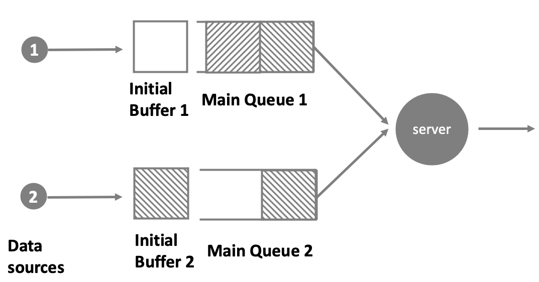
Figure 4: Initial Buffer and Main Queue for LCFS

Similar to what we did in Section III-B, since in the system of M/G/1 type queues with LCFS, there is one initial buffer in each queue, we can thus derive the PAoI for queue $i$ as:

$$\boldsymbol{E}[A_{i}] = \boldsymbol{E}[P_{i}]+\boldsymbol{E}[W_{i}]+\boldsymbol{E}[I_{i}]+\boldsymbol{E}[G_{i}]$$ (8)

$$= \frac{1}{\mu_{i}}+\frac{p_{i}}{\lambda_{i}(1-p_{i})}+\frac{2}{\lambda_{i}}-\frac{1}{\lambda_{i}}\boldsymbol{E}[e^{-\lambda_{i}W_{i}}],$$

for all $i\in\{1,...,k\},$ where we abuse our notation here by letting $p_{i}$ be the steady state probability that the initial buffer is full (notice that in Section III we used it as the probability that the buffer is full). Now we introduce the method of finding $p_{i}$’s by providing Lemma 6 for the case of $k=1$ first.

Lemma 6.

For the M/G/1 queue with LCFS of $k=1$, the probability that the initial buffer is full is given by $p_{1}=\frac{\lambda_{1}}{\mu_{1}}-1+\psi_{1}(\lambda_{1})$, where $\psi_{1}(u)$ is the LST of the service time.

Proof:

From Figure 5 we find that a busy period of the initial buffer always occurs when the server is processing, and ends when the service is complete. Suppose the processing time of a packet is $P_{1}=u$, then by Campbell’s Theorem [32], the busy period of the initial buffer $\hat{W}$ during time $P_{1}=u$ is given by

$$\boldsymbol{E}[\hat{W}|P_{1}=u] = \sum_{m=1}^{\infty}\frac{m}{m+1}ue^{-\lambda_{1}u}\frac{(\lambda_{1}u)^{m}}{m!}$$

$$= u-\frac{1}{\lambda_{1}}+\frac{1}{\lambda_{1}}e^{-\lambda_{1}u}.$$

By unconditioning on $P_{1}=u$ we have $\boldsymbol{E}[\hat{W}]=\int_{0}^{\infty}(u-\frac{1}{\lambda_{1}}+\frac{1}{\lambda_{1}}e^{-\lambda_{1}u})dF_{1}(u)=\frac{1}{\mu_{1}}-\frac{1}{\lambda_{1}}+\frac{\psi_{1}(\lambda_{1})}{\lambda_{1}}$. However, it is important to note that this $\boldsymbol{E}[\hat{W}]$ is the expected busy time of initial buffer during the processing time of a packet. To obtain $p_{i}$, we need the following argument. Suppose $n(t)$ packets have been served during $(0,t]$. Thus the amount of time that the initial buffer being full during $(0,t]$ is $n(t)\boldsymbol{E}[\hat{W}]$. If the queue is stable, we have $n(t)$ converging to $\lambda_{1}t$ as $t\rightarrow\infty.$ Therefore

$$p_{1}=\lim_{t\rightarrow\infty}\frac{n(t)\boldsymbol{E}[\hat{W}]}{t}=\lambda_{1}\boldsymbol{E}[\hat{W}],$$

which is the stationary probability that the initial buffer is full. Note that $\frac{\lambda_{1}}{\mu_{1}}-1+\psi_{1}(\lambda_{1})$ is a legitimate probability as it always lies within $[0,1]$. To show this, from the fact that $\psi_{1}(\lambda_{1})=\int_{0}^{\infty}e^{-\lambda x}dF_{1}(x)\leq 1$, we have $\frac{\lambda_{1}}{\mu_{1}}-1+\psi_{1}(\lambda_{1})\leq\frac{\lambda_{1}}{\mu_{1}}<1$ from stability assumption. Since $\psi_{1}(\lambda_{1})=\int_{0}^{\infty}e^{-\lambda x}dF_{1}(x)\geq\int_{0}^{\infty}(1-\lambda_{1}x)dF_{1}(x)=1-\frac{\lambda_{1}}{\mu_{1}}$, we have $\frac{\lambda_{1}}{\mu_{1}}-1+\psi_{1}(\lambda_{1})\geq 0$. Thus $\frac{\lambda_{1}}{\mu_{1}}-1+\psi_{1}(\lambda_{1})$ is a legitimate probability. ∎

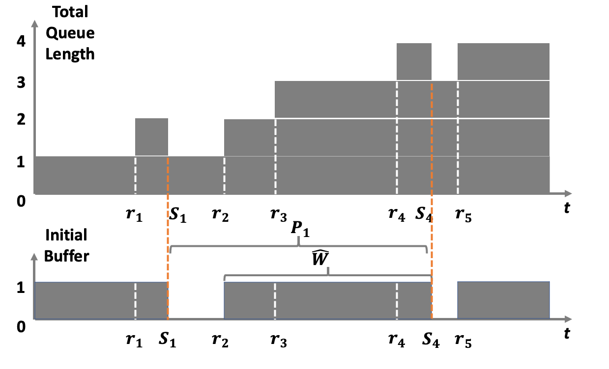
Figure 5: Initial Buffer and Total Queue Length (Including Initial Buffer and Main Queue) for LCFS

Now we discuss the case when $k\geq 2$. Notice that for each packet that is in service, if there is a new arrival from queue 1 occurring during this service time, then the busy period for initial buffer 1 is from the arrival time of this new packet to the completion time of the packet being processed. From Lemma 6, the busy period for initial buffer 1 if a type $i$ packet is being processed when the busy period starts, is given by $\frac{1}{\mu_{i}}-\frac{1}{\lambda_{1}}+\frac{1}{\lambda_{1}}\psi_{i}(\lambda_{1}).$ Thus we have $p_{1}=\sum_{i=1}^{k}\lambda_{i}(\frac{1}{\mu_{i}}-\frac{1}{\lambda_{1}}+\frac{1}{\lambda_{1}}\psi_{i}(\lambda_{1}))$ .

To get the probability $p_{i}$ for queue $i\geq 2$, we use the idea introduced by Kella and Yechiali [39]. We merge the queues with priority higher than $i$ as one class $\mathcal{C}_{ai}$ and the other queues as another class $\mathcal{C}_{bi}$ by letting $\lambda_{ai}=\sum_{j=1}^{i-1}\lambda_{j}$, $\lambda_{bi}=\sum_{j=i}^{k}\lambda_{j}$, $\rho_{ai}=\sum_{j=1}^{i-1}\rho_{j}$ and $\rho_{bi}=\sum_{j=i}^{k}\rho_{j}$. We also let $F_{ai}(x)=\sum_{j=1}^{i-1}\frac{\lambda_{j}}{\lambda_{ai}}F_{j}(x)$ be the service time distribution for packets from class $\mathcal{C}_{ai}$, with mean $\boldsymbol{E}[P_{ai}]$ and $F_{bi}(x)=\sum_{j=i}^{k}\frac{\lambda_{j}}{\lambda_{bi}}F_{j}(x)$ be the service time distribution for packets from class $\mathcal{C}_{bi}$, with mean $\boldsymbol{E}[P_{bi}].$ Notice that the busy period of initial buffer $i$ ends only when there is no packet from class $\mathcal{C}_{ai}$. We now classify the busy periods of server (the time period during which the server is continuously serving packets) into two types. One type of busy period $V_{ai}$ starts with processing a packet from $\mathcal{C}_{ai}$, and ends when there is no packet of from $\mathcal{C}_{ai}$ left in the system. The other type of busy period $V_{bi}$ starts with processing a packet from $\mathcal{C}_{bi}$, and also ends when there is no packet from $\mathcal{C}_{ai}$ left in the system. If no packet from $\mathcal{C}_{ai}$ arrives during processing the first packet in $V_{bi}$, then the length of $V_{bi}$ is just $P_{bi}$. If one packet from $\mathcal{C}_{ai}$ arrives during processing the first packet in $V_{bi}$, then after the processing the first packet, a busy period $V_{ai}$ is followed. Similar to the analysis in [39, 33] and what we did in Section III-A, by conditioning on service time of the first packet in a busy period, the LST of $V_{ai}$ and $V_{bi}$, denoted as $\tilde{V}_{ai}(s)$ and $\tilde{V}_{bi}(s)$, are given as

$$\tilde{V}_{ai}(s) = \psi_{ai}(s+\lambda_{ai}-\lambda_{ai}\tilde{V}_{ai}(s))$$ (9)

and

$$\tilde{V}_{bi}(s) = \psi_{bi}(s+\lambda_{ai}-\lambda_{ai}\tilde{V}_{ai}(s)),$$ (10)

where $\psi_{ai}(s)$ is the LST of $F_{ai}(x)$ and $\psi_{bi}(s)$ is the LST of $F_{bi}(x).$ By taking the derivative of $\tilde{V}_{ai}(s)$ and $\tilde{V}_{bi}(s)$ at $s=0$, the expected length of server’s busy periods can be given as

$$\boldsymbol{E}[V_{ai}] = \frac{\boldsymbol{E}[P_{ai}]}{1-\rho_{ai}},$$

and

$$\boldsymbol{E}[V_{bi}] = \frac{\boldsymbol{E}[P_{bi}]}{1-\rho_{ai}}.$$

Note that busy period $V_{bi}$ always starts by serving a packet from $\mathcal{C}_{bi}$, thus we know

$$\boldsymbol{P}(system\ in\ V_{bi}) = \lambda_{bi}\frac{\boldsymbol{E}[P_{bi}]}{1-\rho_{ai}}.$$

Since when the server is busy, it is either in busy period $V_{ai}$ or $V_{bi}$ , we have

$$\boldsymbol{P}(system\ in\ V_{ai}) = \sum_{j=1}^{k}\rho_{j}-\lambda_{bi}\frac{\boldsymbol{E}[P_{bi}]}{1-\rho_{ai}}=\hat{\lambda}_{ai}\frac{\boldsymbol{E}[P_{ai}]}{1-\rho_{ai}},$$

where

$$\hat{\lambda}_{ai} = \frac{\sum_{j=1}^{k}\rho_{j}-\lambda_{bi}\frac{\boldsymbol{E}[P_{bi}]}{1-\rho_{ai}}}{\frac{\boldsymbol{E}[P_{ai}]}{1-\rho_{ai}}}$$ (11)

is the “arrival rate” of busy period $V_{ai}.$ We now use $F_{ai}^{V}(x)$ and $F_{bi}^{V}(x)$ to denote the CDF of $V_{ai}$ and $V_{bi}$. From Lemma 6 we know that during busy period $V_{ai}$, the time period of initial buffer being busy is given as

$$\boldsymbol{E}[\hat{W}_{ai}] = \int_{0}^{\infty}(u-\frac{1}{\lambda_{i}}+\frac{1}{\lambda_{i}}e^{-\lambda_{i}u})dF_{ai}^{V}(u)$$ (12)

$$= \frac{\boldsymbol{E}[P_{ai}]}{1-\rho_{ai}}-\frac{1}{\lambda_{i}}+\frac{1}{\lambda_{i}}\tilde{V}_{ai}(\lambda_{i}).$$

Similarly, we have $\boldsymbol{E}[\hat{W}_{bi}]=\frac{\boldsymbol{E}[P_{bi}]}{1-\rho_{ai}}-\frac{1}{\lambda_{i}}+\frac{1}{\lambda_{i}}\tilde{V}_{bi}(\lambda_{i}).$ In many cases where $\tilde{V}_{ai}(\lambda_{i})$ and $\tilde{V}_{bi}(\lambda)$ cannot be solved analytically, numerical methods such as bisection method or Newton’s method (see [40]) can be applied to find the roots numerically. From the same argument in Lemma 6, we have

$$p_{i} = \hat{\lambda}_{ai}\boldsymbol{E}[\hat{W}_{ai}]+\lambda_{bi}\boldsymbol{E}[\hat{W}_{bi}].$$ (13)

Next we introduce the process of obtaining $\boldsymbol{E}[e^{-\lambda_{i}W_{i}}]$ for Equation (8). Notice that $\hat{W}_{ai}$ is the length of initial buffer being full during period $V_{ai}$. Similar to the argument in Lemma 6, we have

$$\boldsymbol{E}[e^{-s\hat{W}_{ai}}|V_{ai}=t]$$

$$= \int_{0}^{t}e^{-sx}\sum_{m=1}^{\infty}\frac{mx^{m-1}}{t^{m}}e^{-\lambda_{i}t}\frac{(\lambda_{i}t)^{m}}{m!}dx+e^{-\lambda_{i}t}$$

$$= \int_{0}^{t}e^{-sx}e^{-\lambda_{i}t}\sum_{m=1}^{\infty}x^{m-1}\frac{(\lambda_{i})^{m}}{(m-1)!}dx+e^{-\lambda_{i}t}$$

$$= e^{-\lambda_{i}t}\frac{\lambda_{i}}{\lambda_{i}-s}(e^{(\lambda_{i}-s)t}-1)+e^{-\lambda_{i}t}$$

$$= \frac{\lambda_{i}}{\lambda_{i}-s}e^{-st}-\frac{s}{\lambda_{i}-s}e^{-\lambda_{i}t}.$$

By unconditioning on $V_{ai}=t$ we have

$$\boldsymbol{E}[e^{-s\hat{W}_{ai}}] = \frac{\lambda_{i}}{\lambda_{i}-s}\tilde{V}_{ai}(s)-\frac{s}{\lambda_{i}-s}\tilde{V}_{ai}(\lambda_{i}),$$

and

$$\boldsymbol{E}[e^{-s\hat{W}_{bi}}] = \frac{\lambda_{i}}{\lambda_{i}-s}\tilde{V}_{bi}(s)-\frac{s}{\lambda_{i}-s}\tilde{V}_{bi}(\lambda_{i}).$$

Using L’Hospital rule taking the limit $s\rightarrow\lambda_{i}$, we have

$$\boldsymbol{E}[e^{-\lambda_{i}\hat{W}_{ai}}] = -\lambda_{i}\tilde{V}_{ai}^{{}^{\prime}}(\lambda_{i})+\tilde{V}_{ai}(\lambda_{i}),$$ (14)

and

$$\boldsymbol{E}[e^{-\lambda_{i}\hat{W}_{bi}}] = -\lambda_{i}\tilde{V}_{bi}^{{}^{\prime}}(\lambda_{i})+\tilde{V}_{bi}(\lambda_{i}).$$ (15)

From the formula of $\tilde{V}_{ai}(s)$ and $\tilde{V}_{bi}(s)$ given above we have

$$\tilde{V}_{ai}^{{}^{\prime}}(\lambda_{i}) = \frac{\psi_{ai}^{{}^{\prime}}(\lambda_{i}+\lambda_{ai}-\lambda_{ai}\tilde{V}_{ai}(\lambda_{i}))}{1+\lambda_{ai}\psi_{ai}^{{}^{\prime}}(\lambda_{i}+\lambda_{ai}-\lambda_{ai}\tilde{V}_{ai}(\lambda_{i}))},$$ (16)

and

$$\tilde{V}_{bi}^{{}^{\prime}}(\lambda_{i})$$ (17)

$$= \psi_{bi}^{{}^{\prime}}(\lambda_{i}+\lambda_{ai}-\lambda_{ai}\tilde{V}_{ai}(\lambda_{i}))(1-\lambda_{ai}\tilde{V}_{ai}^{{}^{\prime}}(\lambda_{i})).$$

Notice that $W_{i}$ is the busy period of the initial buffer for each age peak, and only ($1-p_{i}$) portion of arrivals in queue $i$ incur age peaks, so the “arrival rate” for $W_{i}$ is $\lambda_{i}(1-p_{i})$. Since $\hat{W}_{i}$ is the busy period of initial buffer during each $V_{ai}$ and $V_{bi}$ with arrival rate $\hat{\lambda}_{ai}$ and $\lambda_{bi}$ respectively, from the fact that $\lambda_{bi}=\sum_{j=i}^{k}\lambda_{j}\geq\lambda_{i}(1-p_{i})$, we have the following relationship

$$\hat{\lambda}_{ai}\boldsymbol{E}[e^{-\lambda_{i}\hat{W}_{ai}}]+\lambda_{bi}\boldsymbol{E}[e^{-\lambda_{i}\hat{W}_{bi}}]$$

$$= \lambda_{i}(1-p_{i})\boldsymbol{E}[e^{-\lambda_{i}W_{i}}]+(\hat{\lambda}_{ai}+\lambda_{bi}-\lambda_{i}(1-p_{i})).$$

Therefore,

$$\boldsymbol{E}[e^{-\lambda_{i}W_{i}}] = \frac{1}{\lambda_{i}(1-p_{i})}\bigg{[}\hat{\lambda}_{ai}\boldsymbol{E}[e^{-\lambda_{i}\hat{W}_{ai}}]+\lambda_{bi}\boldsymbol{E}[e^{-\lambda_{i}\hat{W}_{bi}}]$$ (18)

$$-(\hat{\lambda}_{ai}+\lambda_{bi}-\lambda_{i}(1-p_{i}))\bigg{]}.$$

A closed-form formula of PAoI in M/G/1 type queues with LCFS is then given in the following theorem.

Theorem 7.

The PAoI of queue $i$ in M/G/1 system with LCFS is given by $\boldsymbol{E}[A_{i}]=\frac{1}{\mu_{i}}+\frac{1}{\lambda_{i}(1-p_{i})}-\frac{1}{\lambda_{i}^{2}(1-p_{i})}\bigg{[}\hat{\lambda}_{ai}(-\lambda_{i}\tilde{V}_{ai}^{{}^{\prime}}(\lambda_{i})+\tilde{V}_{ai}(\lambda_{i})-1)+\lambda_{bi}(-\lambda_{i}\tilde{V}_{bi}^{{}^{\prime}}(\lambda_{i})+\tilde{V}_{bi}(\lambda_{i})-1)\bigg{]},$ where $\tilde{V}_{ai}(s)=\psi_{ai}(s+\lambda_{ai}-\lambda_{ai}\tilde{V}_{ai}(s))$, $\tilde{V}_{bi}(s)=\psi_{bi}(s+\lambda_{ai}-\lambda_{ai}\tilde{V}_{ai}(s))$, $p_{i}=\hat{\lambda}_{ai}\left[\frac{\boldsymbol{E}[P_{ai}]}{1-\rho_{ai}}-\frac{1}{\lambda_{i}}+\frac{1}{\lambda_{i}}\tilde{V}_{ai}(\lambda_{i})\right]+\lambda_{bi}\left[\frac{\boldsymbol{E}[P_{bi}]}{1-\rho_{ai}}-\frac{1}{\lambda_{i}}+\frac{1}{\lambda_{i}}\tilde{V}_{bi}(\lambda_{i})\right]$, and $\hat{\lambda}_{ai}=\frac{\sum_{j=1}^{k}\rho_{j}-\lambda_{bi}\frac{\boldsymbol{E}[P_{bi}]}{1-\rho_{ai}}}{\frac{\boldsymbol{E}[P_{ai}]}{1-\rho_{ai}}}$.

Proof:

To obtain the exact PAoI for queue $i$ of M/G/1 system with LCFS, we first solve $\tilde{V}_{ai}(\lambda_{i})$ and $\tilde{V}_{bi}(\lambda_{i})$ using Equation (9) and (10). And all the required components for computing $\boldsymbol{E}[e^{-\lambda_{i}W_{i}}]$ in Equation (18) can be obtained from Equations (11) - (17). After that the PAoI of queue $i$ can be obtained using Equation (8). ∎

Note here that this approach of calculating PAoI of queue $i$ in M/G/1 type system LCFS can still be applied even when the number of queues $k$ is large. The numerical test of this approach will be provided in Section V.

IV-C Discussion of the Single Queue Systems

The LST of PAoI for single queue with LCFS was provided in [3], however its expression is quite involved (see Equation (99) in [3]). Here we use our approach introduced in Subsection IV-B to provide a concise expression for PAoI of M/G/1/LCFS queue in the following corollaries. Since we only have one queue here, for simplicity of the notation, in this subsection we remove the subscript of each variable.

Corollary 8.

The PAoI of M/G/1/LCFS is given by $\boldsymbol{E}[A]=\frac{1}{\mu}+\frac{1}{\lambda}+\frac{\frac{1}{\mu}+\psi^{{}^{\prime}}(\lambda)}{2-\frac{\lambda}{\mu}-\psi(\lambda)}$, where $\psi(\lambda)$ is the LST of service time.

Proof:

Since we know $\boldsymbol{E}[e^{-\lambda\hat{W}}]=-\lambda\psi^{{}^{\prime}}(\lambda)+\psi(\lambda)$ from Equation (15) and $\boldsymbol{E}[e^{-\lambda W}]=\frac{\boldsymbol{E}[e^{-\lambda\hat{W}}]-p}{1-p}$ from Equation (18), also from Lemma 6 we know $p=\frac{\lambda}{\mu}-1+\psi(\lambda)$, we have our corollary proved. ∎

Corollary 9.

The PAoI of M/M/1/LCFS is given by $\boldsymbol{E}[A]=\frac{1}{\lambda}+\frac{1}{\mu}+\frac{2\lambda\mu+\lambda^{2}}{(\lambda+\mu)(\mu^{2}+\lambda\mu-\lambda^{2})}$.

It is shown in [7] that M/M/1/$2^{*}$ system has a smaller PAoI than M/M/1/2 and M/M/1/1 systems. Interestingly, we find that the PAoI in M/G/1/$2^{*}$ system is no greater than that in M/G/1/LCFS system, as shown in the following theorem.

Theorem 10.

The PAoI in M/G/1/$2^{*}$ system is no greater than that in M/G/1/LCFS system, for any $\rho=\frac{\lambda}{\mu}<1$.

Proof:

It is shown in [41] that the PAoI in M/G/1/$2^{*}$ system is given by $\boldsymbol{E}[A^{M/G/1/2^{*}}]=\frac{2}{\mu}+\frac{1}{\lambda}+\psi^{{}^{\prime}}(\lambda).$ Using the result of Corollary 8, we have

$$\boldsymbol{E}[A^{M/G/1/LCFS}]-\boldsymbol{E}[A^{M/G/1/2^{*}}]$$

$$= \frac{1}{\mu}+\frac{1}{\lambda}+\frac{\frac{1}{\mu}+\psi^{{}^{\prime}}(\lambda)}{2-\frac{\lambda}{\mu}-\psi(\lambda)}-\left(\frac{2}{\mu}+\frac{1}{\lambda}+\psi^{{}^{\prime}}(\lambda)\right)$$

$$= \left(\frac{1}{\mu}+\psi^{{}^{\prime}}(\lambda)\right)\frac{\frac{\lambda}{\mu}+\psi(\lambda)-1}{2-\frac{\lambda}{\mu}-\psi(\lambda)}.$$

We first have $\frac{1}{\mu}+\psi^{{}^{\prime}}(\lambda)=\frac{1}{\mu}-\boldsymbol{E}[Pe^{-\lambda P}]=\boldsymbol{E}[P]-\boldsymbol{E}[Pe^{-\lambda P}]\geq 0$. Then from the facts that

$$\frac{\lambda}{\mu}+\psi(\lambda) = \lambda\boldsymbol{E}[P]+\boldsymbol{E}[e^{-\lambda P}]$$

$$\geq \lambda\boldsymbol{E}[P]+\boldsymbol{E}[1-\lambda P]=1$$

and $\frac{\lambda}{\mu}+\psi(\lambda)<2$, we have $\boldsymbol{E}[A^{M/G/1/LCFS}]\geq\boldsymbol{E}[A^{M/G/1/2^{*}}].$ ∎

We now show that LCFS is actually not the optimal service discipline for minimizing PAoI among all the non-preemptive work-conserving service disciplines. To do this, we simply consider the case of exponential service. The PAoI of FCFS in this case is given by $\boldsymbol{E}[A^{FCFS}]=\frac{1}{\lambda}+\frac{1}{\mu}+\frac{\lambda}{\mu(\mu-\lambda)}$. We then have

$$\boldsymbol{E}[A^{FCFS}]-\boldsymbol{E}[A^{LCFS}]$$

$$= \frac{\lambda}{\mu(\mu-\lambda)}-\frac{2\lambda\mu+\lambda^{2}}{(\lambda+\mu)(\mu^{2}+\lambda\mu-\lambda^{2})}$$

$$= \frac{-\lambda^{4}+\lambda^{3}\mu+3\lambda^{2}\mu^{2}-\lambda\mu^{3}}{\mu(\mu-\lambda)(\lambda+\mu)(\mu^{2}+\lambda\mu-\lambda^{2})}.$$

If we let $\mu=1$ in the formula above, we have $\boldsymbol{E}[A^{FCFS}]-\boldsymbol{E}[A^{LCFS}]=\frac{-\lambda^{4}+\lambda^{3}+3\lambda^{2}-\lambda}{(1-\lambda)(\lambda+1)(1+\lambda-\lambda^{2})}$. By numerically solving it we know that $\boldsymbol{E}[A^{FCFS}]\leq\boldsymbol{E}[A^{LCFS}]$ when $0\leq\lambda<\lambda^{*}=0.3111,$ and $\boldsymbol{E}[A^{FCFS}]>\boldsymbol{E}[A^{LCFS}]$ when $1>\lambda>\lambda^{*}$, which is also shown in Figure 7(a). Similarly, in Section V, we will show that LCFS is not the optimal service discipline for the multi-queue case either, when the objective is to minimize PAoI of each queue.

This result contradicts to the conclusion in [42] since it was correctly proven in Theorem 3 of [42], that for an arbitrary sample path (arrival and service times realizations), LCFS always results in a smaller age process $\Delta(t)$ for $t\in[0,\infty)$ than FCFS. The authors of [42] then concluded that PAoI under LCFS is smaller than that under FCFS, which is not accurate. The reason is that the average age peaks (up to time $T$) is not a non-decreasing functional (that is defined in [42]) of the age process $\Delta(t)$ during $t\in[0,T)$. Figure 6 shows the age functions of FCFS and LCFS under the same sample path, where LCFS always has a smaller age $\Delta(t)$ than FCFS, but FCFS can have smaller average age peaks than LCFS. In fact, PAoI is an expected value conditioning on those packets that cause age peaks (they are also called informative packets [43, 44]). Under FCFS, all the data packets arriving into the system are informative, but the informative packets under LCFS are only a subset of all the data packets. As shown in Figure 6, the LCFS age function may not have peaks at all the time instances the FCFS age function has peaks. This explains why FCFS can sometimes have smaller PAoI than LCFS. However, the advantage of applying FCFS may only come from the definition of metric PAoI. We will discuss more about the metric PAoI in Subsection IV-D.

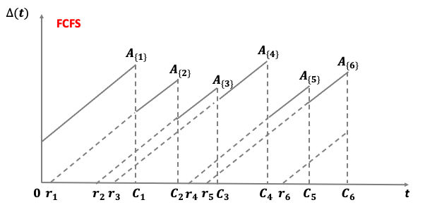
(a) PAoI under FCFS. The first 6 packets result in 6 age peaks

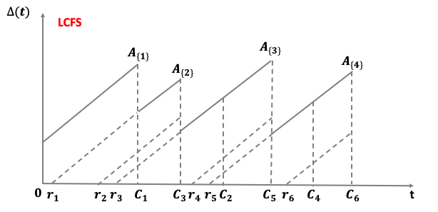
(b) PAoI under LCFS. The first 6 packets result in 4 age peaks

Figure 6: PAoI under FCFS and LCFS

In fact, FCFS can also sometimes have a smaller PAoI than M/M/1/$2^{*}$ system, as shown in Figure 7(b). This is also due the special property of the metric PAoI, since in M/M/1/$2^{*}$ system, not all the packets eventually result in age peaks. In Section V we will show that for the multi-queue case, having buffer with size one can sometimes result a larger PAoI than FCFS.

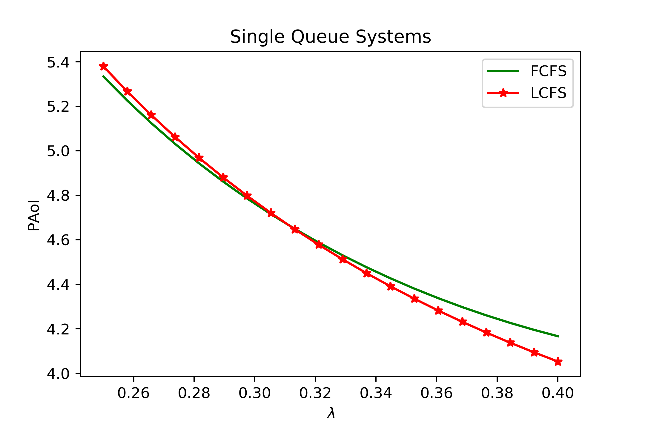
(a) FCFS versus LCFS

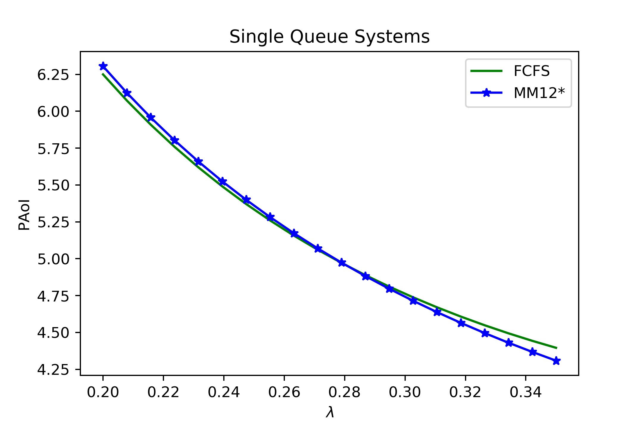
(b) FCFS versus $M/M/1/2^{*}$

Figure 7: FCFS for M/M/1 Queue with $\mu=1$

IV-D Discussion on the Metric PAoI

We show in Subsection IV-C that FCFS can sometimes have a smaller PAoI than LCFS or the single buffer system. However, any advantage of FCFS may only come from the special definition of PAoI. FCFS may not have real advantage over LCFS, since LCFS always results in a smaller age than FCFS for an arbitrary sample path all the time (as correctly proven in [42]). Considering PAoI as the objective metric may lead us to the conclusion of LCFS being non-optimal, which, to some extent, implies that PAoI may not be a perfect metric to measure the information freshness.

In fact, the peak age (not its expected value PAoI) is worth of studying in many senses. First of all, it can be used to characterize age violation penalties (see [7, 45, 46]), especially when the interest is in the worst case (see [47]). Secondly, peak age can be used to derive other age-related metrics such as AoI (see [41, 3]). The metric PAoI however, as the expected value of peak age, is not able to fully characterize the properties of peak age. The maximal peak age (see [48]), peak age distribution (see [46, 47]), or the Laplace-Stieltjes Transform (LST) of peak age (see [49, 41, 3]) may also be interesting metrics to study.

On the other hand, PAoI is also a useful alternative metric to AoI, especially when AoI is difficult to obtain analytically. In many systems, PAoI has a simple form and some classic queueing results can be easily applied to derive PAoI (see [7, 44, 2, 17, 41, 50]). In some cases, PAoI can also be used as a bound or an approximation for AoI (see [51, 2]). PAoI and AoI also perform similarly when changing the traffic rate in many systems (see [7, 41]). As a metric to measure information freshness, a small PAoI means that the average maximal age stays at a low level, which indicates that the system receives frequent update in the long run. While our analysis reveals the limitation of PAoI in some specific settings, more properties of PAoI are worth exploring in the future.

V Numerical Study

In this section we will firstly use a numerical study to verify the exact solutions for M/M/1+$\sum 1^{*}$ that we provided in Section III-A, and then test the bounds of M/G/1+$\sum 1^{*}$ which we provided in Section III-B. We will then verify the exact solution for M/G/1 type queues with LCFS. Besides, we will compare the performance of different service disciplines, and develop our insights based on the numerical studies.

We begin our discussion by comparing simulation results with exact solutions for M/M/1+$\sum 1^{*}$ system with $k=2$. The comparison is done by changing one parameter from $\lambda_{1},\ \lambda_{2},\ \mu_{1}$ and $\mu_{2}$ while keeping the others fixed. The results are shown in Figure 8. From plots in Figure 8 we can see that the simulation results match the exact solutions that we provide in Section III-A, thus verifying our results. Figure 8(a) shows that when we increase the arrival rate for the priority 1 queue, its PAoI is drastically decreased, while PAoI for queue 2 increases constantly. Figure 8(b) shows that if we increase the arrival rate of queue 2, its PAoI will decrease dramatically, while PAoI of queue 1 increases slowly. Figure 8(c) and (d) show that when service rate increases, PAoI for both queues are decreased. Interestingly, we find that when queue 1 has a low service rate, PAoI for both queues will be large, while PAoI of queue 1 is not significantly affected by the service rate change of queue 2. We then test how the average PAoI across queues (i.e., $\frac{1}{k}\sum_{i=1}^{k}\boldsymbol{E}[A_{i}]$) is affected by parameters, which we show in Figure 9. From Figure 9(a) we see that by increasing the service rate of either queue, the average PAoI across queues will be reduced, and increasing the service rate of queue 1 makes this reduction more significant. Figure 9(b) shows that by increasing the arrival rate of queue 2, the average PAoI across queues is decreased. This is because the PAoI for queue 1 is not sensitive to the arrival rate of queue 2, as we also show in Theorem 3. However, when we increase the arrival rate of queue 1, the average PAoI will decrease drastically at the beginning, and increase afterwards. This is because the PAoI of queue 2 increases constantly when we increase $\lambda_{1}$, which we also see from Figure 8(a). Note that although we only discuss the optimization problem of minimizing average PAoI across queues here, since we have the exact solution for PAoI, we could also formulate and solve optimization problems such as minimizing average weighted PAoI (similar to [21]) and minimizing the maximum PAoI (similar to [2]).

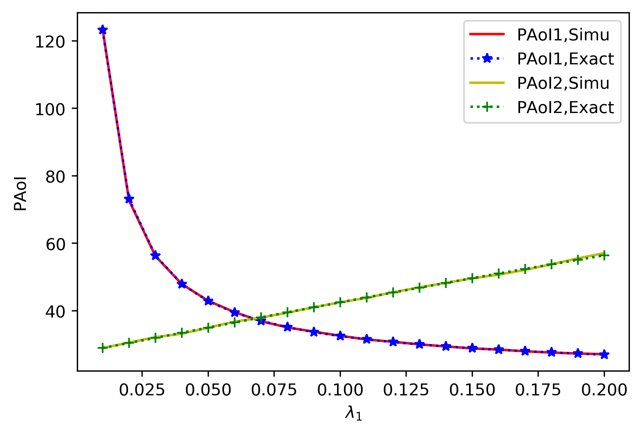
(a) $\mu_{1}=\frac{1}{10},\lambda_{2}=\frac{1}{10},\mu_{2}=\frac{1}{10}$

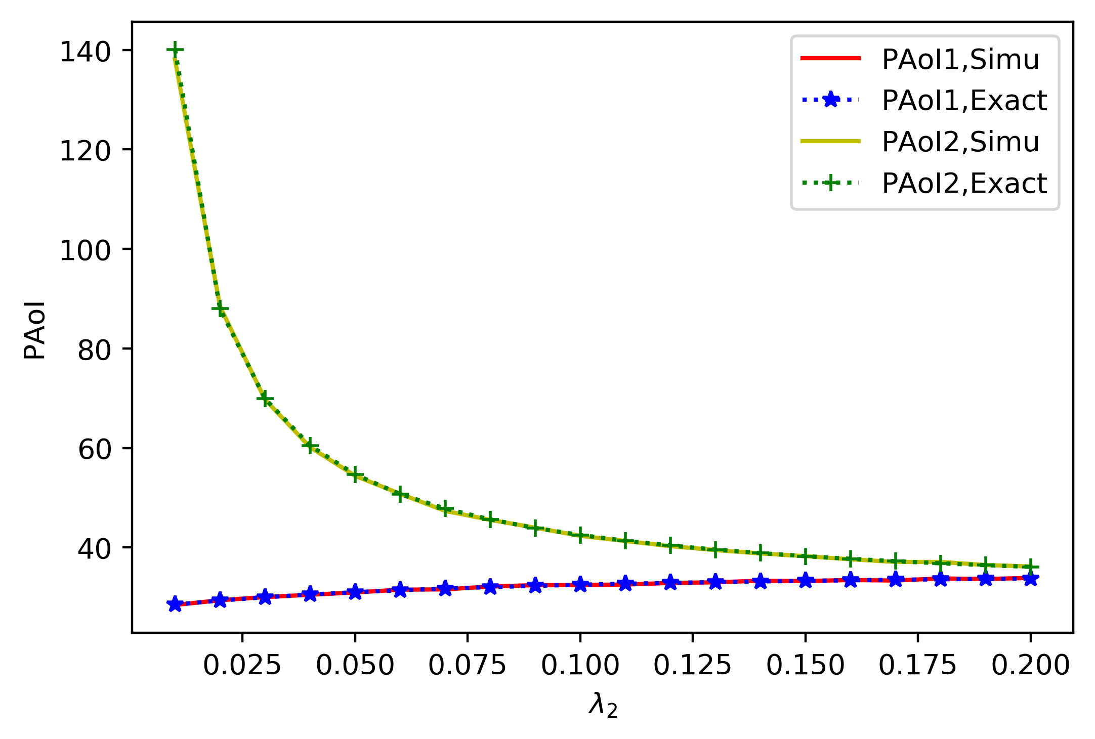
(b) $\lambda_{1}=\frac{1}{10},\mu_{1}=\frac{1}{10},\mu_{2}=\frac{1}{10}$

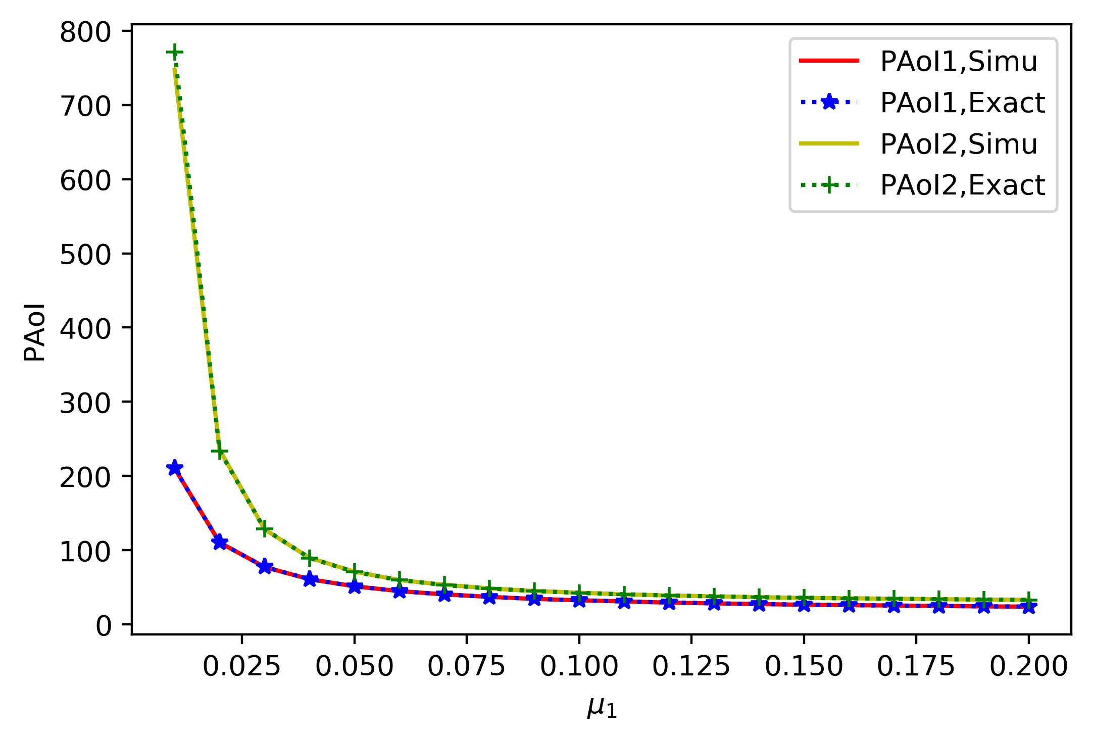
(c) $\lambda_{1}=\frac{1}{10},\lambda_{2}=\frac{1}{10},\mu_{2}=\frac{1}{10}$

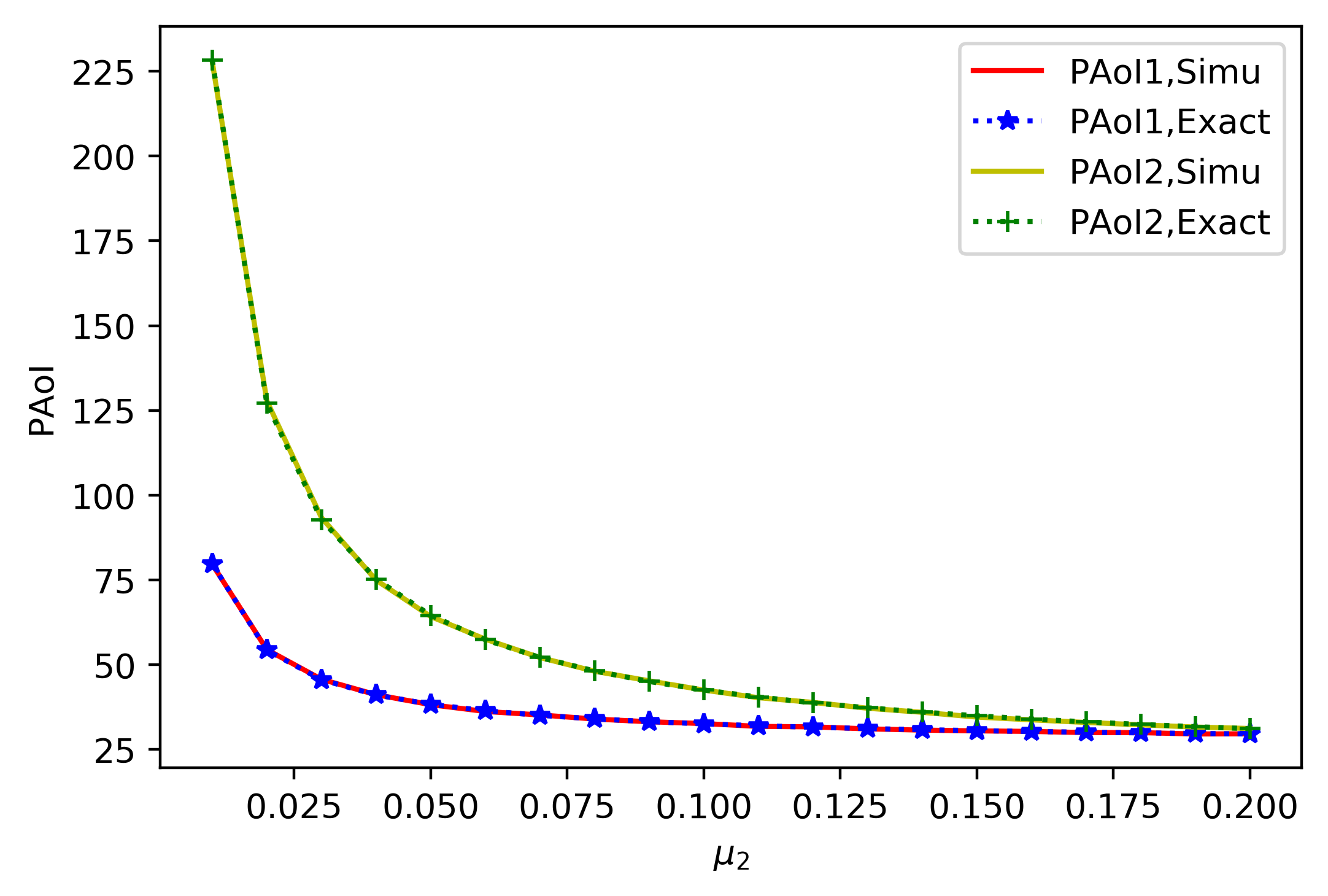
(d) $\lambda_{1}=\frac{1}{10},\mu_{1}=\frac{1}{10},\lambda_{2}=\frac{1}{10}$

Figure 8: M/M/1+$\sum 1^{*}$ Type Queues with Buffer Size One

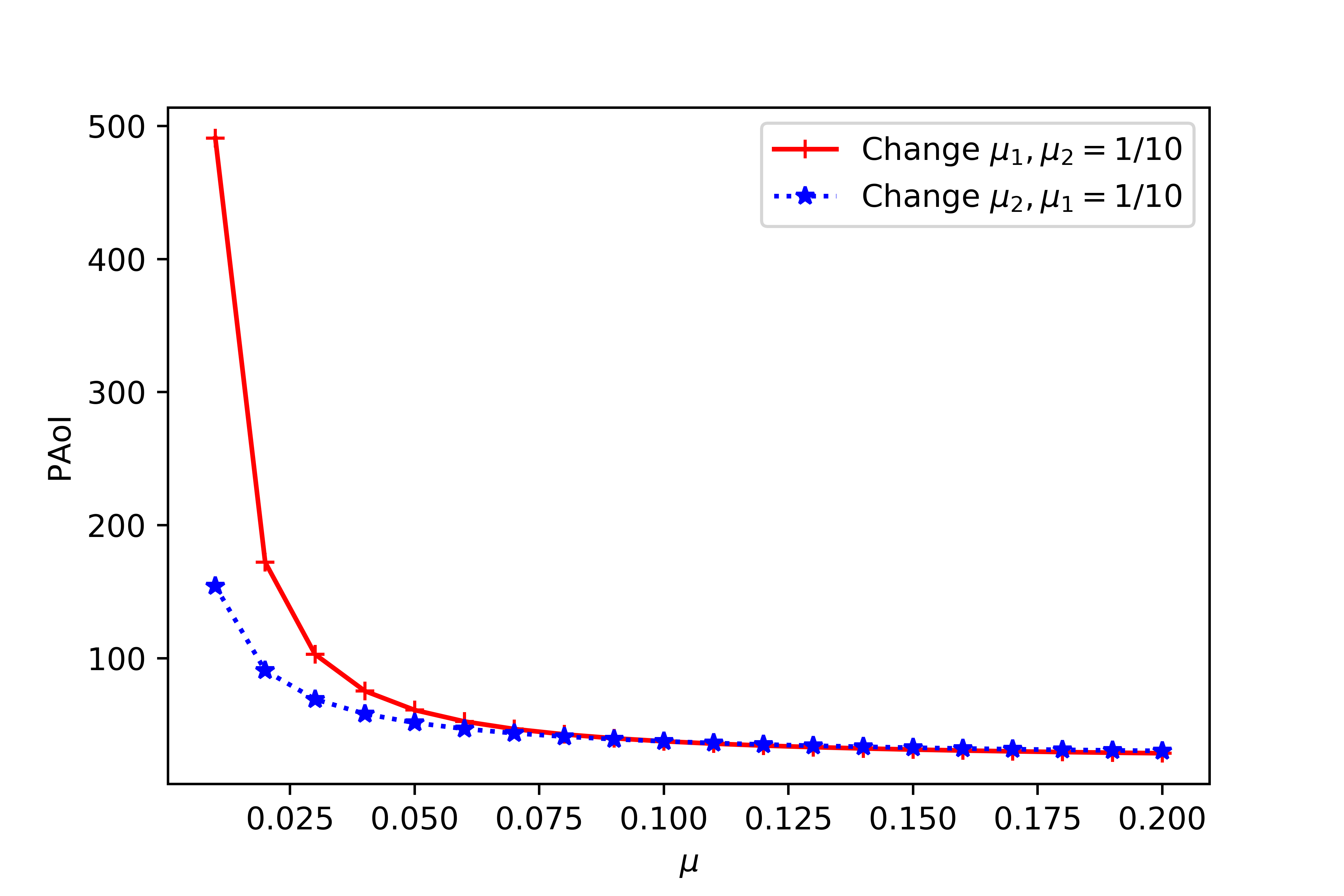
(a) $\lambda_{1}=\frac{1}{10},\lambda_{2}=\frac{1}{10}$

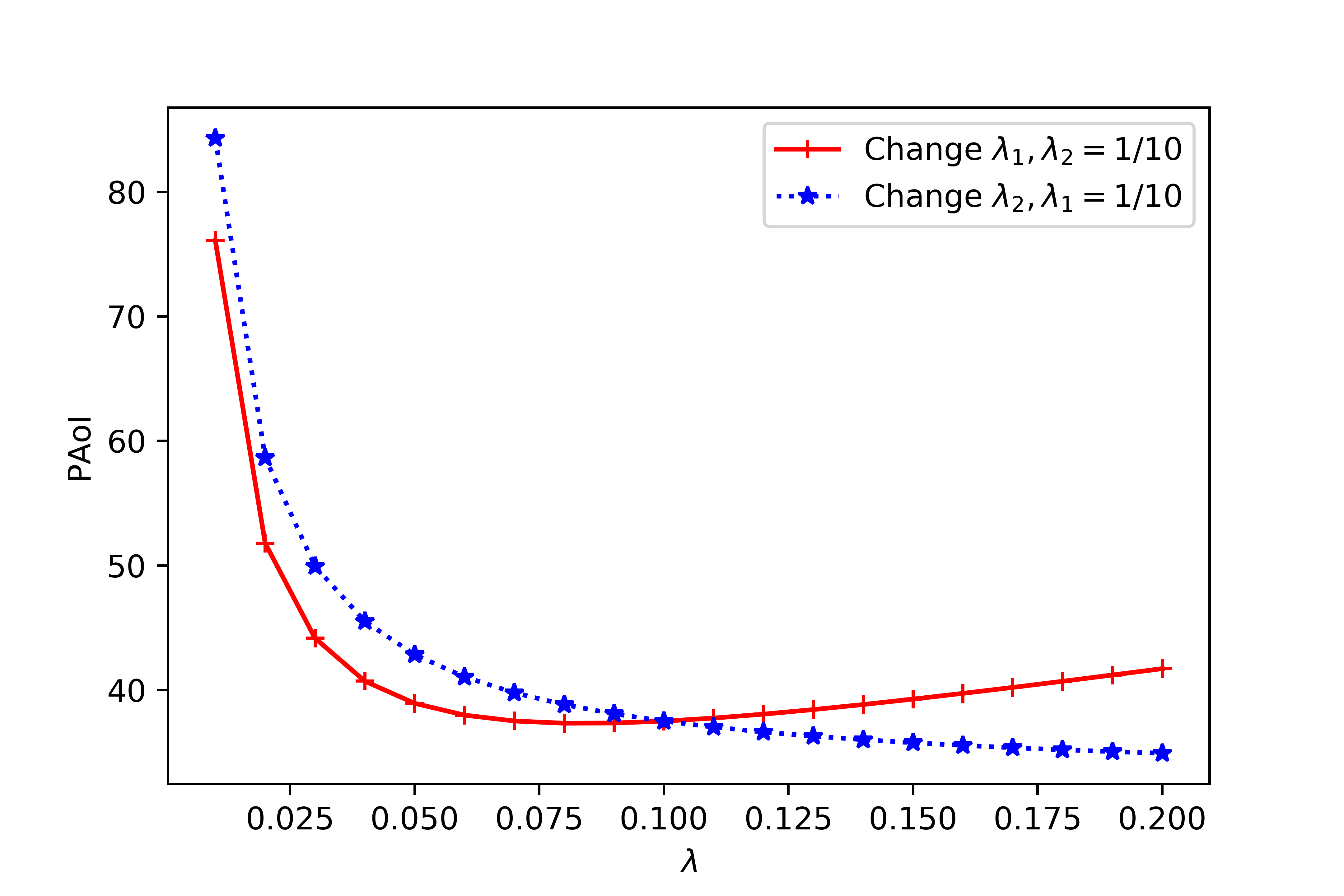
(b) $\mu_{1}=\frac{1}{10},\mu_{2}=\frac{1}{10}$

Figure 9: Average PAoI of M/M/1+$\sum 1^{*}$ Queues with Buffer Size One

Next we consider queues with general service times. The bounds for M/G/1+$\sum 1^{*}$ type queues with buffer size one and $k=3$ are shown in Figure 10, where the bounds are provided by Inequality (4). We test the bounds by letting service time follow exponential, uniform and gamma distributions. Note that in Figure 10 we provide the bounds for exponential service case too, although we have the exact solution for PAoI when service times are exponential. We find from Figure 10 that Inequality (4) serves as a decent approximation for the actual PAoI since the bounds and simulation curves for all queues are close. The three service distributions in Figure 10 have the same mean but the LST of these distributions vary from each other. From our discussion in Section III we find that the probability $p_{i}$ is related to the LST of service time. Therefore, different service time distributions result in different probability $p_{i},$ and further result in different PAoI.

Then we consider queues with infinite buffer size. The exact PAoI and simulation results for M/G/1 type queues with LCFS are shown in Figure 11. We also test the cases for exponential, uniform and gamma distributed service times. In Figure 11 we see that the exact PAoI that we provide in Subsection IV-B match the simulation results. We also find that in M/G/1 type queues with LCFS, by increasing the arrival rate of queue 1, PAoI of queue 1 is significantly reduced, and PAoI for lower priority queues is increased at the same time. We do not present the numerical test for M/G/1 queues with FCFS here, as its analysis is exact and also straightforward.

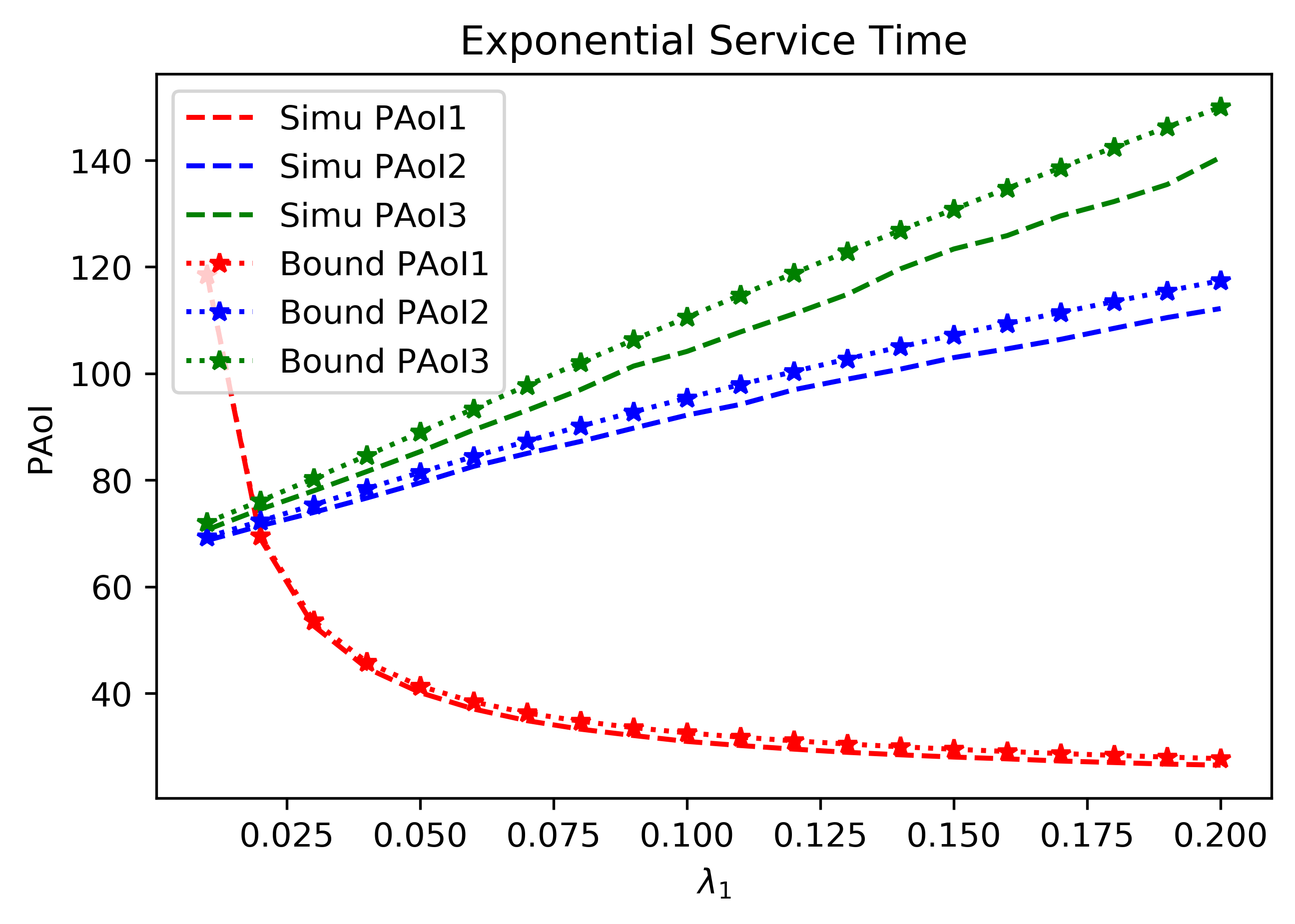
(a) $\lambda_{2}=\lambda_{3}=\frac{1}{30}$, $P_{1},P_{2},P_{3}\sim exp(\frac{1}{10})$

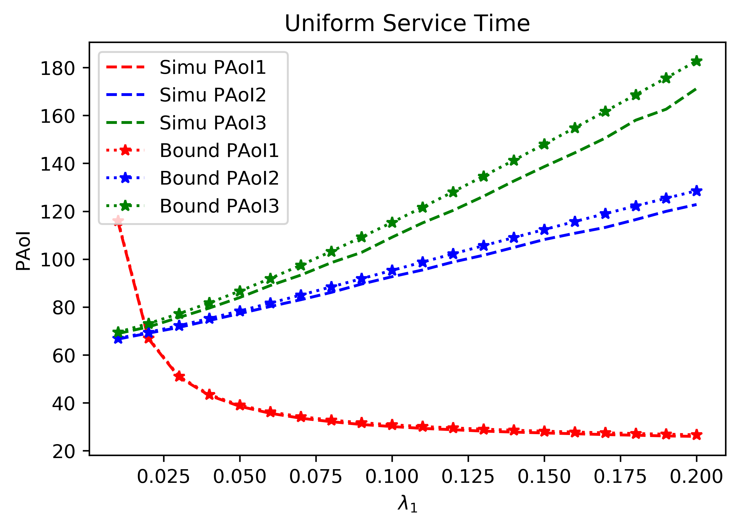
(b) $\lambda_{2}=\lambda_{3}=\frac{1}{30},$ $P_{1},P_{2},P_{3}\sim Unif(0,20)$

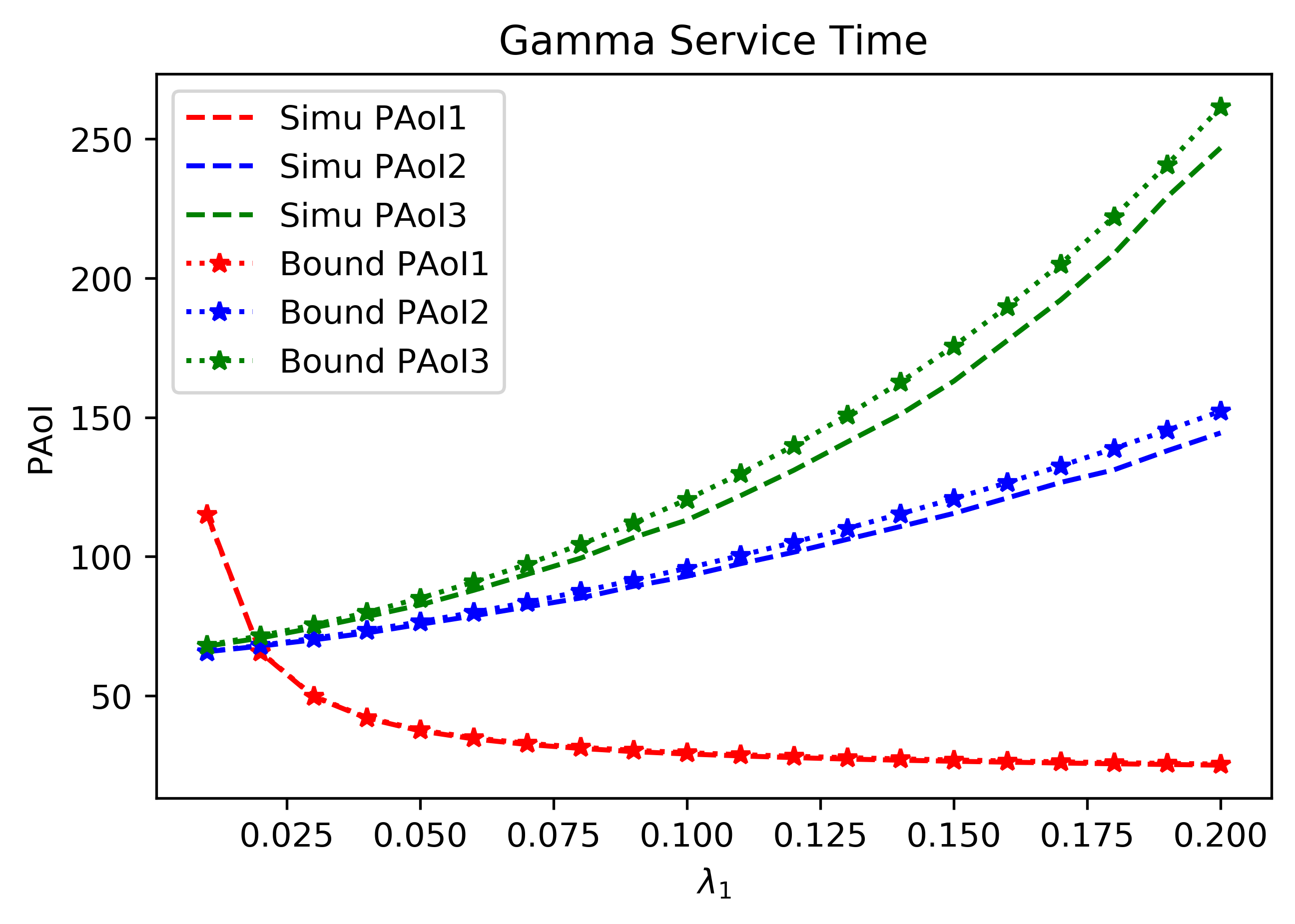
(c) $\lambda_{2}=\lambda_{3}=\frac{1}{30},$ $P_{1},P_{2},P_{3}\sim Gamma(10,1)$

Figure 10: Bounds for M/G/1+$\sum 1^{*}$ Type Queues with Buffer Size One

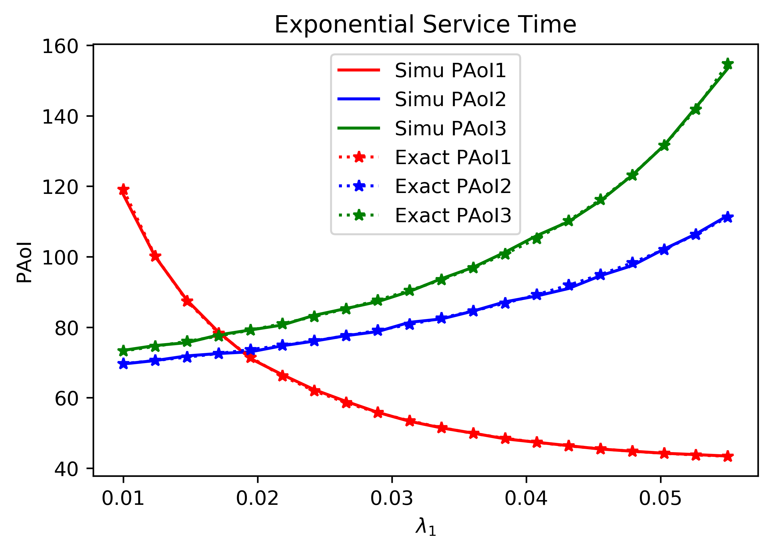
(a) $\lambda_{2}=\lambda_{3}=\frac{1}{50},$ $P_{1},P_{2},P_{3}\sim exp(\frac{1}{10})$

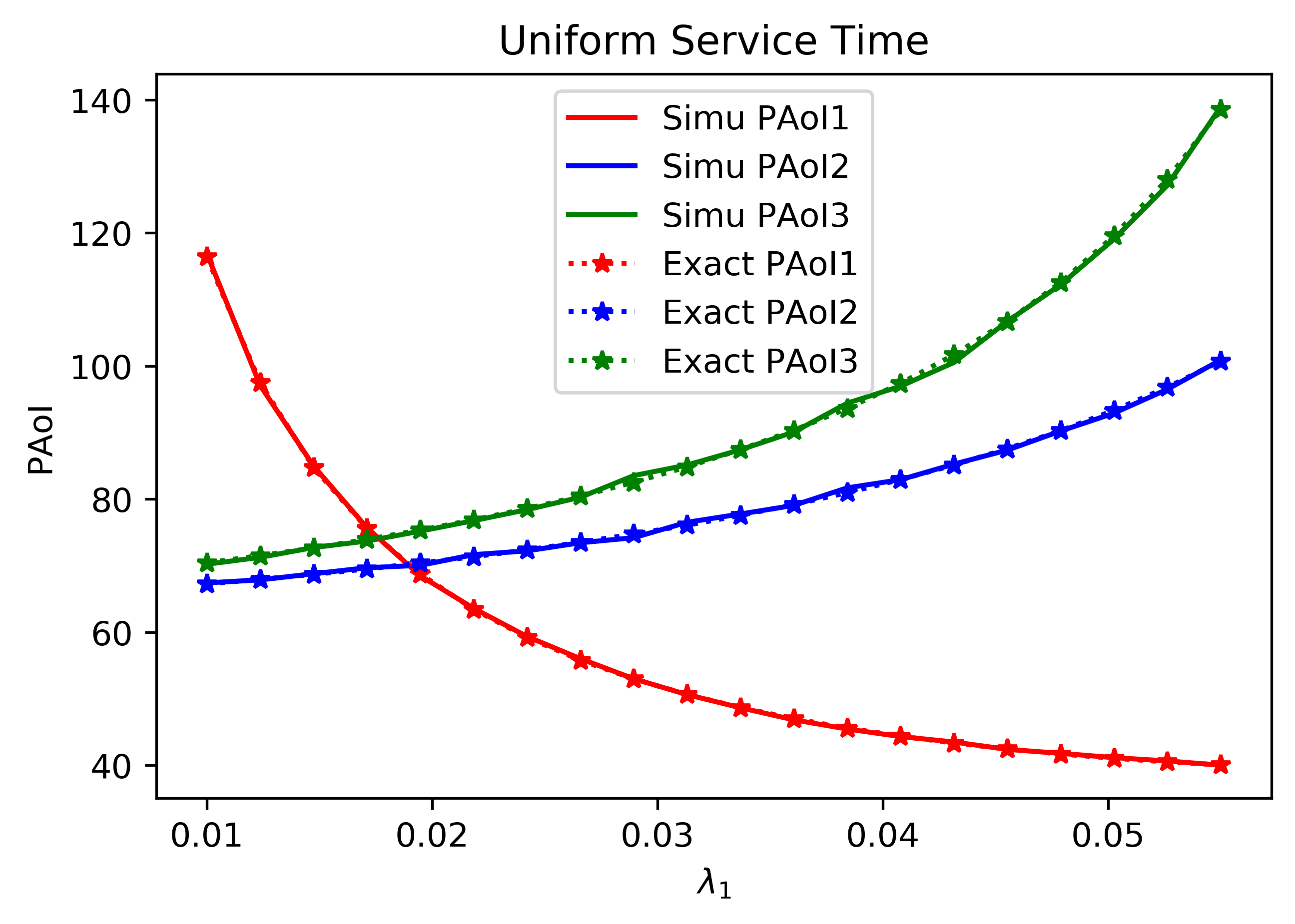
(b) $\lambda_{2}=\lambda_{3}=\frac{1}{50},$$P_{1},P_{2},P_{3}\sim Unif(0,20)$

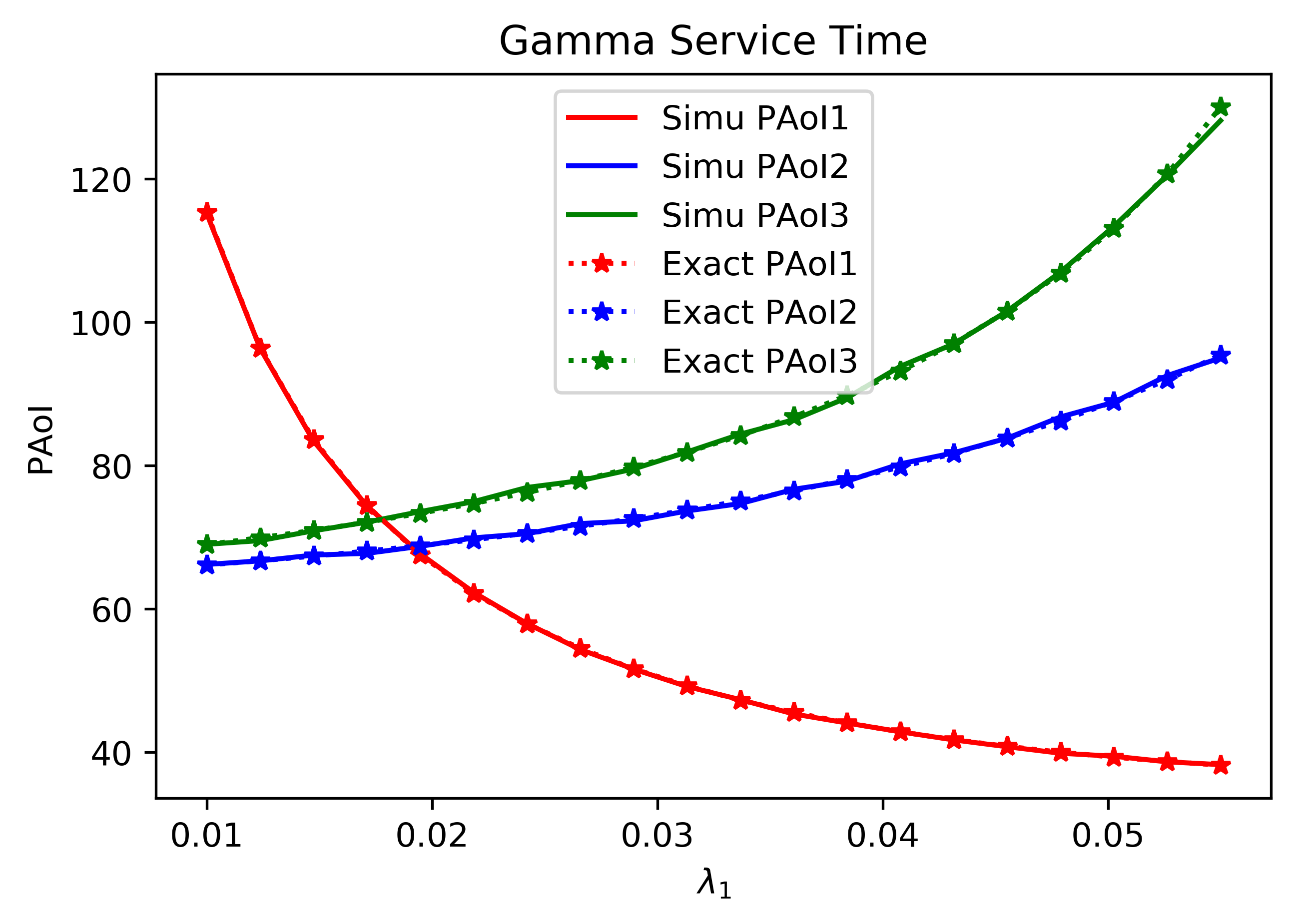
(c) $\lambda_{2}=\lambda_{3}=\frac{1}{50},$$P_{1},P_{2},P_{3}\sim Gamma(10,1)$

Figure 11: M/G/1 Type Queues with LCFS

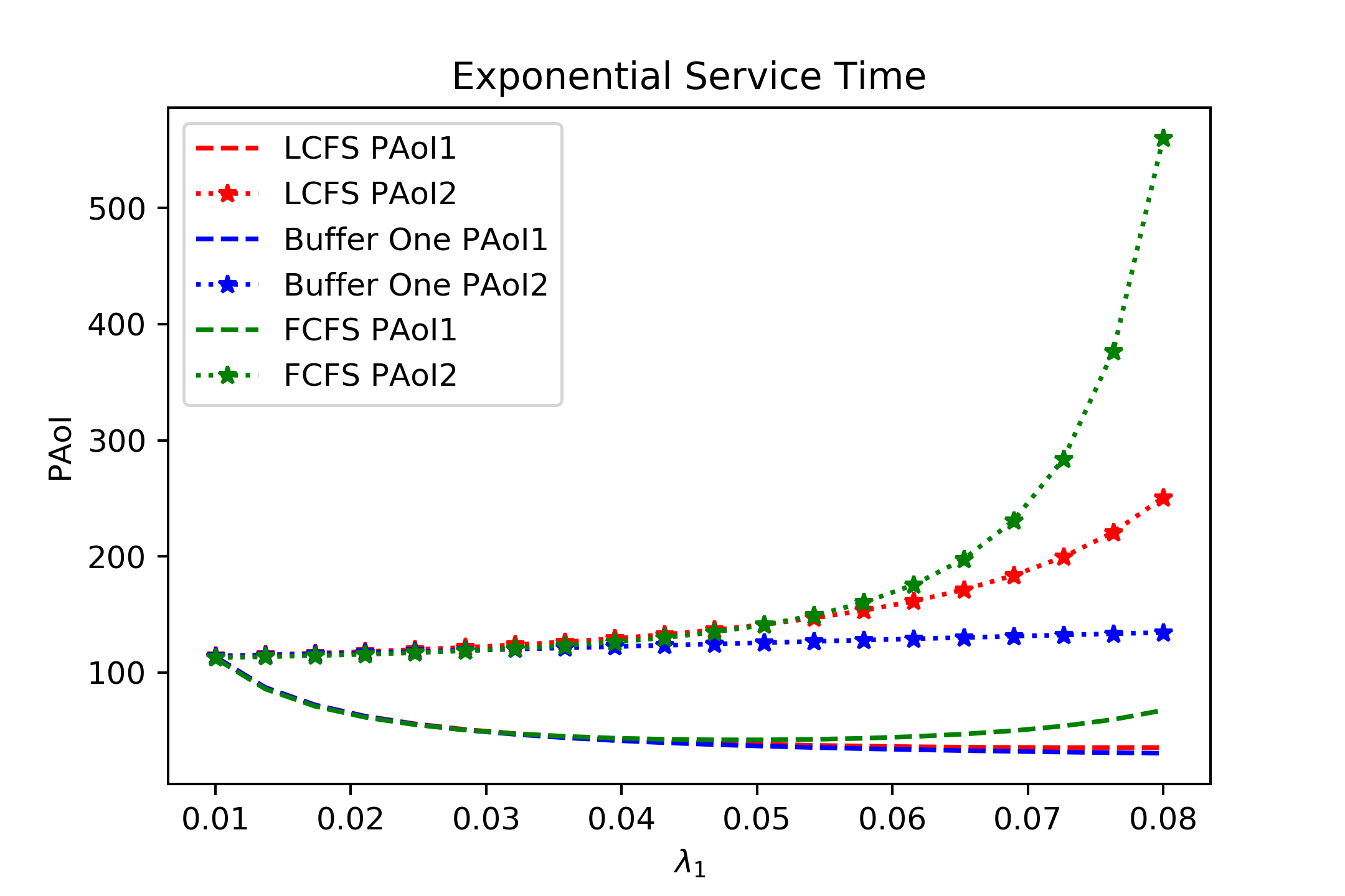
(a) $\lambda_{2}=\frac{1}{100},\mu_{1}=\mu_{2}=\frac{1}{10}$

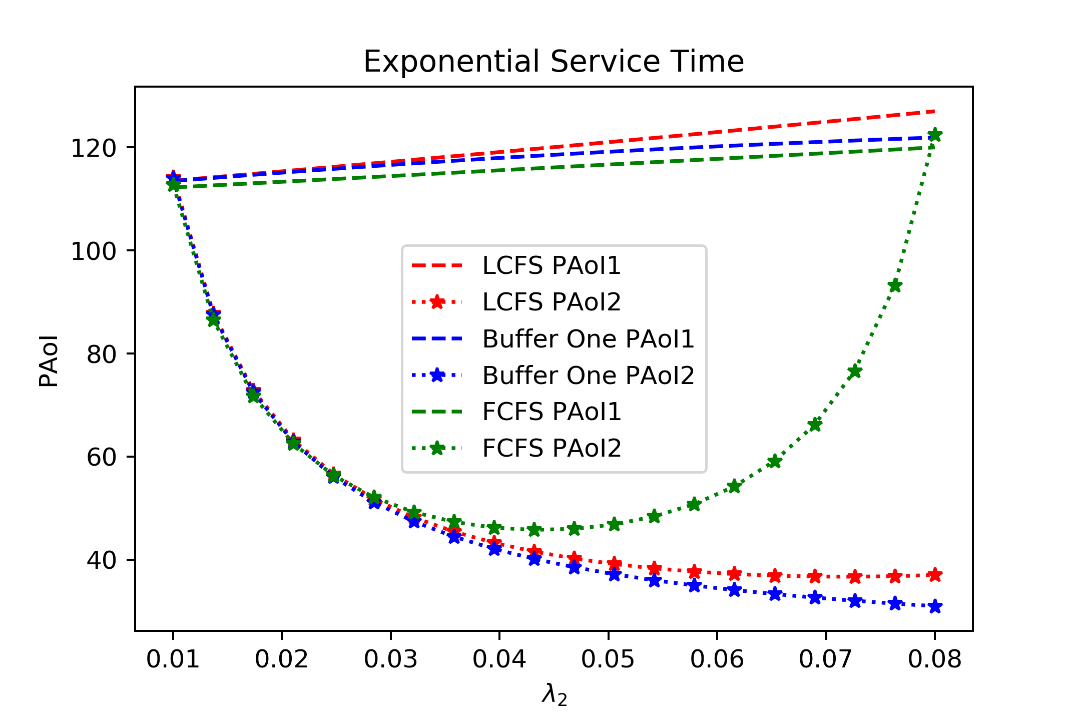
(b) $\lambda_{1}=\frac{1}{100},\mu_{1}=\mu_{2}=\frac{1}{10}$

Figure 12: PAoI under Different Service Disciplines

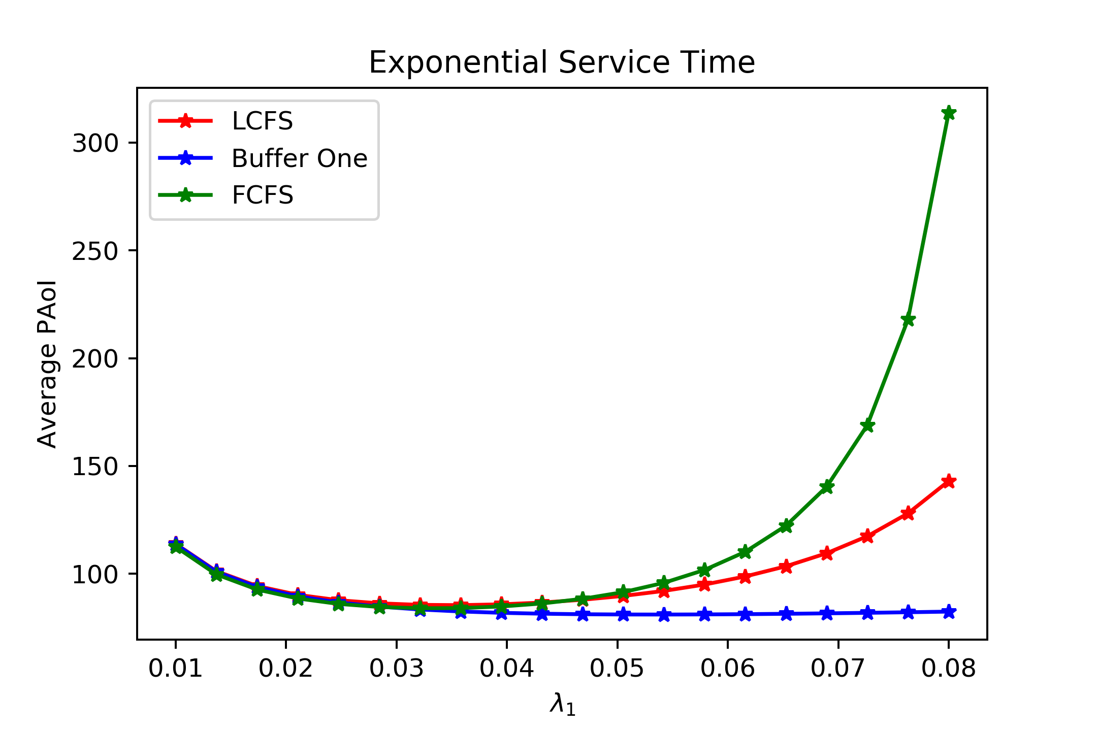
(a) $\lambda_{2}=\frac{1}{100},\mu_{1}=\mu_{2}=\frac{1}{10}$

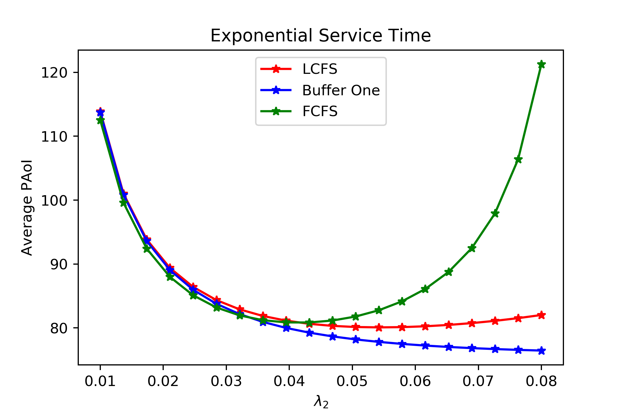
(b) $\lambda_{1}=\frac{1}{100},\mu_{1}=\mu_{2}=\frac{1}{10}$

Figure 13: Average PAoI Across Queues under Different Service Disciplines

Next we address PAoI by comparing the single buffer size case against infinite buffer size cases under FCFS and LCFS. In fact, since in the M/G/1 system with infinite buffer size, if we keep replacing the packets in buffers with new arrivals, then there is at most one packet waiting in each queue, therefore the system will act exactly the same as M/G/1+$\sum 1^{*}$ system. So here we consider the PAoI under M/G/1+$\sum 1^{*}$and M/G/1 with FCFS and LCFS altogether. In Figure 12 we plot the PAoI for each queue in the case of $k=2$, and in Figure 13 we plot the average PAoI across all queues ($\frac{1}{2}\sum_{i=1}^{2}\boldsymbol{E}[A_{i}]$). From Figure 12 we see that under FCFS, LCFS and M/M/1+$\sum 1^{*}$, PAoI of queue 2 is sensitive to the change of $\lambda_{1}$, however PAoI of queue 1 is less sensitive to $\lambda_{2}$. This is because the PAoI for queue 2 highly depends on the busy time of queue 1. For FCFS, the PAoI increases greatly when arrival rate becomes large. This is because under FCFS, every packet that arrive to the system needs to be processed, and increasing arrival rate enlarges the average queue size, causing packets to wait a longer time. From the average PAoI across queues shown in Figure 13, we can see that increasing the arrival rate for the high priority queue enlarges the PAoI much faster than increasing $\lambda_{2}$. It indicates that when designing the priority for queues to minimize average PAoI across queues, the one with the lowest traffic intensity should be allocated with the highest priority. We also proved this result in Section IV for M/G/1 queues with FCFS.

Also, it is interesting to observe that having a single-sized buffer at each queue is not always the optimal strategy to minimize PAoI, as we observe from Figure 12 and Figure 13. This fact can be seen more clearly in Figure 12(b) and Figure 13(b) when the traffic intensity of queue 2 is higher. In Figure 12(b), the PAoI of queue 1 under FCFS is lower than that under the other two policies. In Figure 13(b), FCFS results in lower average PAoI than the other two policies when the traffic intensity is low. This result also indicates that LCFS is not the optimal policy among all work-conserving non-preemptive policies when minimizing PAoI. However, as we mentioned in Section IV, the advantage of FCFS may only come from the special property of the metric PAoI.

We now compare the simulation performance of the priority queue policy (which we introduce in this paper), Age-based Max-Weight Policy from [52]) and Randomized Policy with Weights from [21] in M/M/1/$1+\sum 1^{*}$ system. Under the Age-based Max-Weight Policy, at every time $t$ the server becomes available, it selects the non-empty queue with the highest weighted age reduction, i.e., $\max_{i}\beta_{i}(\Delta_{i}(t)-W_{i}(t))$, where $\beta_{i}$ is a constant weight, $\Delta_{i}(t)$ is the age for queue $i$, and $W_{i}(t)$ is the waiting time of the packet in buffer $i$. Under the Randomized Policy with Weights, the server would pick queue $i$ with probability $\frac{\beta_{i}}{\sum_{i\in\mathcal{E}(t)}\beta_{i}}$, where $\mathcal{E}(t)$ is the set of non-empty queues at time $t$. The simulation results for these three policies in a two-queue system with $\beta_{1}=0.8$ and $\beta_{2}=0.2$ are provided in Figure 14. As we see from Figure 14(a), when the traffic intensity of queue 1 is large, the priority queue policy has similar performance to the other two policies on queue 1, but the priority queue policy causes a higher PAoI for queue 2. This is because the priority queue policy has a stronger preference on queue 1 than the other two policies. Under the priority queue policy, queue 2 can only be served when queue 1 is empty, whereas queue 2 can still be served when both queues are non-empty under the other two policies. When traffic intensity of queue 2 is large, the priority queue policy results in a slightly smaller PAoI for queue 1 than the Randomized Policy with Weights, as we can see from Figure 14(b). It is because in this two-queue case, the priority queue policy can be regarded as the Randomized Policy with $\beta_{1}=1$ and $\beta_{2}=0$. Therefore under the priority queue policy, queue 1 is given higher preference than that under the Randomized Policy with $\beta_{1}=0.8$ and $\beta_{2}=0.2$. Like we mentioned in Section I, there could be data sources which have information more important or time-sensitive than the other data sources. The priority queue policy actually helps reduce the PAoI of these data sources by assigning them with high static priorities. When considering the average PAoI across queues, as shown in Figure 14(c) and (d), priority queue policy can result in a slightly smaller average PAoI than the Randomized Policy with $\beta_{1}=0.8$ and $\beta_{2}=0.2$, if high priority is assigned to the queue with low traffic intensity. This also implies that in a system where traffic intensities of queues are distinct, high priority is recommended to be given to the low traffic queue to reduce the average PAoI over queues.

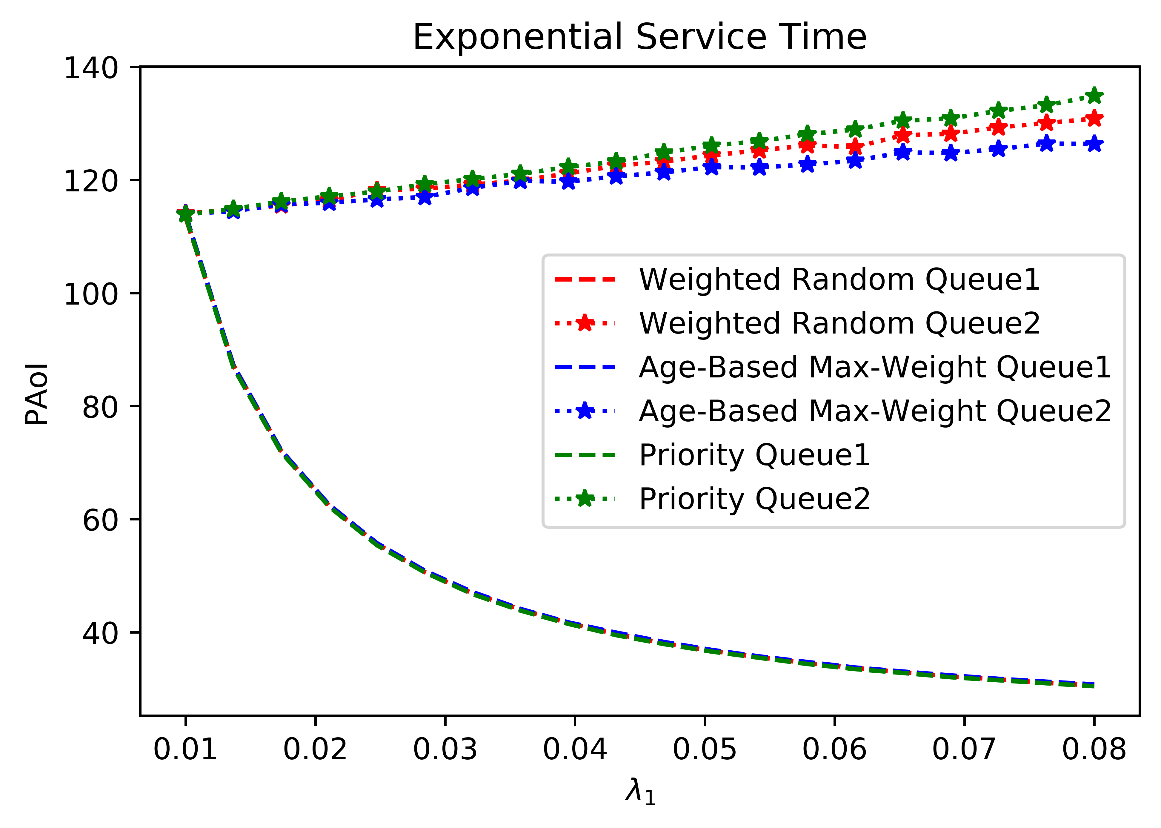
(a) $\lambda_{2}=\frac{1}{100},\mu_{1}=\mu_{2}=\frac{1}{10}$

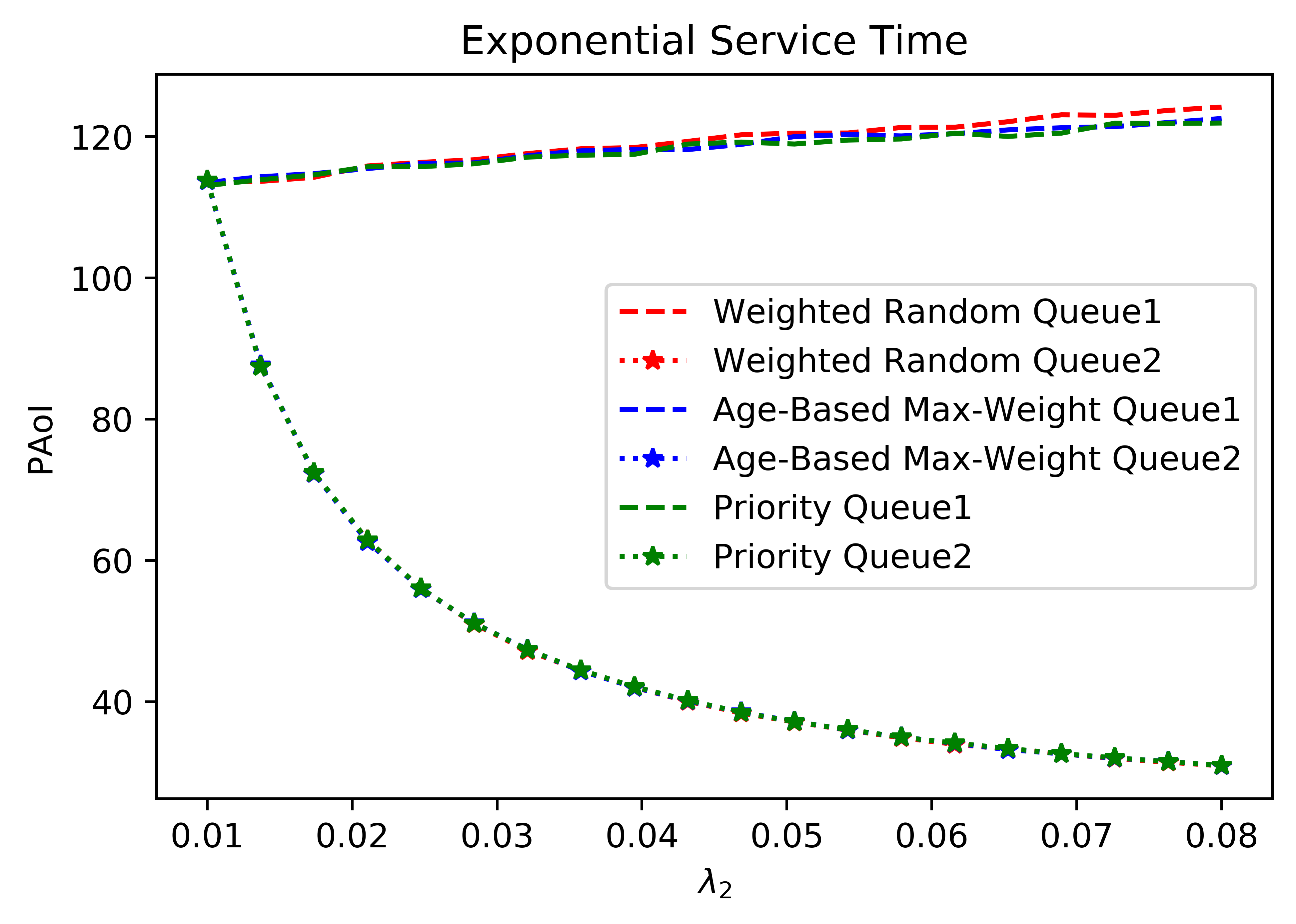
(b) $\lambda_{1}=\frac{1}{100},\mu_{1}=\mu_{2}=\frac{1}{10}$

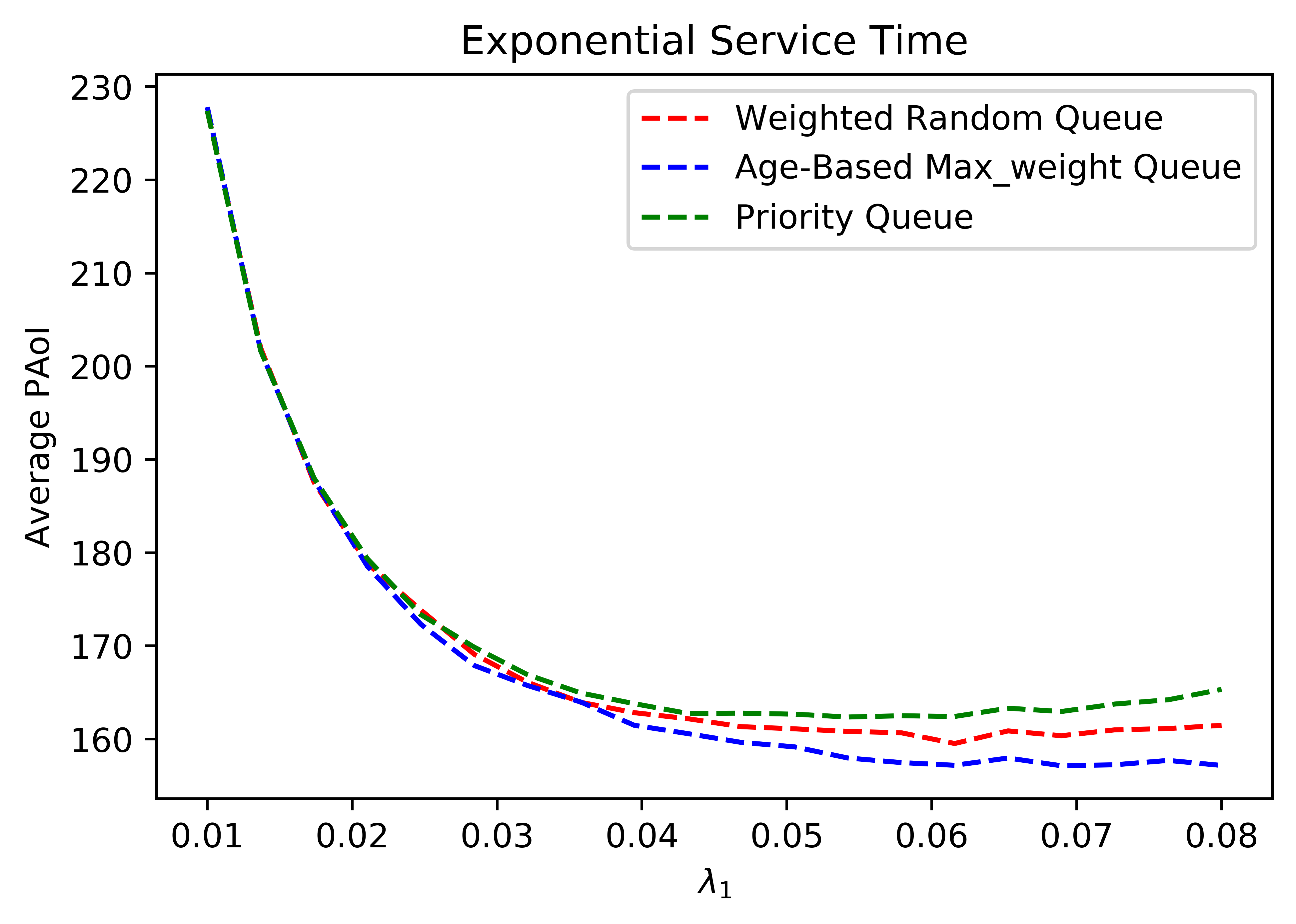
(c) $\lambda_{2}=\frac{1}{100},\mu_{1}=\mu_{2}=\frac{1}{10}$

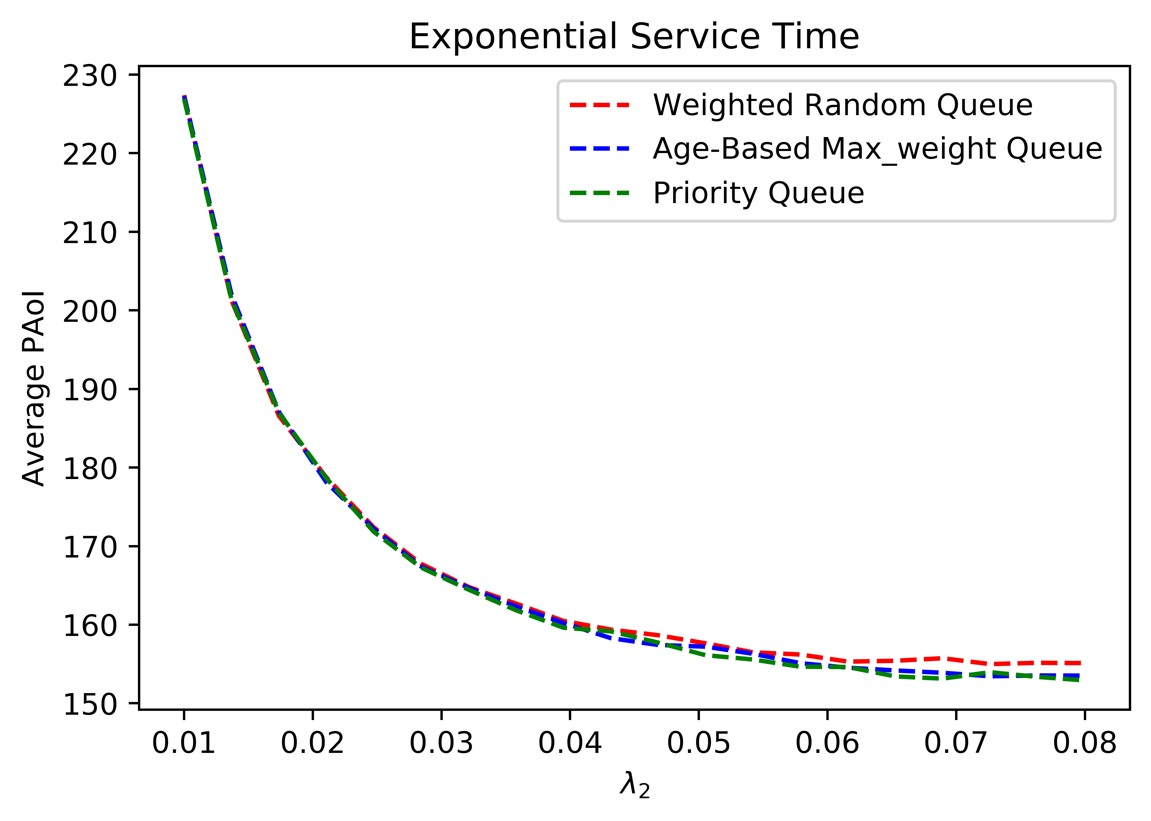
(d) $\lambda_{1}=\frac{1}{100},\mu_{1}=\mu_{2}=\frac{1}{10}$

Figure 14: Policy Comparison

VI Concluding Remarks and Future Work

In this research we considered a multi-class queueing system where each class of data source generates packets according to a Poisson process and a single processor uses a static priority scheme to serve packets. We characterized the PAoI for such a system under two situations: (i) when the buffer size for each queue is one; (ii) when the buffer size for each queue is infinite and service disciplines within each queue can be FCFS or LCFS. We obtained exact expressions for PAoI in case (i) when the service times are exponential, and bounds (which serve as excellent approximations) for case (i) when service times are generally distributed. The method of obtaining PAoI for case (i) becomes cumbersome when the number of queues is large. For case (ii) with general service times, we provided the exact methods for calculating PAoI, and this method can be applied when the number of queues is large.

Using PAoI results, we made a few observations that are useful in determining priorities, service disciplines and sampling rates. We found that LCFS is not the optimal service discipline in minimizing PAoI, and we also found that systems with buffer size one at each queue does not always provide smaller PAoI than the systems with infinite buffer size. These are due to the special definition of the metric PAoI. We further discussed the merits and limitations of the metric PAoI.

From both analytical and numerical results, we showed that for minimizing the average PAoI across queues, it is beneficial to give higher priorities to queues with lower traffic intensities. Besides, we found that the PAoI of queues with low priorities are more sensitive to the packet arrival rate of high priority queues. Increasing the arrival rate for one queue, while reducing the PAoI for this certain data source, would significantly increase the PAoI of queues with lower priorities.

Since in this paper we mainly focus on static queue priorities, in our future work we will consider a system with dynamic priorities. Besides, in smart manufacturing systems where the status of machines changes over time, sampling with a time-varying rate is also possible and it is interesting to consider the PAoI with time-varying arrival rates. Moreover, the variance of PAoI is also useful in measuring the data freshness in real-time systems, and the distribution of PAoI is also of interest. Thus, there are numerous opportunities for research in the area of PAoI for multi-priority queues.

References

- [1] S. Kaul, R. Yates, and M. Gruteser, “Real-time status: How often should one update?,” in INFOCOM, 2012 Proceedings IEEE, pp. 2731–2735, IEEE, 2012.
- [2] L. Huang and E. Modiano, “Optimizing age-of-information in a multi-class queueing system,” in 2015 IEEE International Symposium on Information Theory (ISIT), pp. 1681–1685, IEEE, 2015.
- [3] Y. Inoue, H. Masuyama, T. Takine, and T. Tanaka, “A general formula for the stationary distribution of the age of information and its application to single-server queues,” IEEE Transactions on Information Theory, vol. 65, no. 12, pp. 8305–8324, 2019.
- [4] E. Masry, “Poisson sampling and spectral estimation of continuous-time processes,” IEEE Transactions on Information Theory, vol. 24, no. 2, pp. 173–183, 1978.
- [5] E. Najm, R. Nasser, and E. Telatar, “Content based status updates,” IEEE Transactions on Information Theory, 2019.
- [6] A. Maatouk, M. Assaad, and A. Ephremides, “Age of information with prioritized streams: When to buffer preempted packets?,” in 2019 IEEE International Symposium on Information Theory (ISIT), pp. 325–329, IEEE, 2019.
- [7] M. Costa, M. Codreanu, and A. Ephremides, “On the age of information in status update systems with packet management,” IEEE Transactions on Information Theory, vol. 62, no. 4, pp. 1897–1910, 2016.
- [8] P. Zou, O. Ozel, and S. Subramaniam, “Waiting before serving: A companion to packet management in status update systems,” IEEE Transactions on Information Theory, vol. 66, no. 6, pp. 3864–3877, 2020.
- [9] D. Theodoratos and M. Bouzeghoub, “Data currency quality factors in data warehouse design.,” in DMDW, p. 15, 1999.
- [10] M. Bouzeghoub, “A framework for analysis of data freshness,” in Proceedings of the 2004 international workshop on Information quality in information systems, pp. 59–67, ACM, 2004.
- [11] M. Al-Fares, S. Radhakrishnan, B. Raghavan, N. Huang, and A. Vahdat, “Hedera: dynamic flow scheduling for data center networks.,” in Nsdi, vol. 10, pp. 89–92, 2010.
- [12] L. M. Vaquero and L. Rodero-Merino, “Finding your way in the fog: Towards a comprehensive definition of fog computing,” ACM SIGCOMM Computer Communication Review, vol. 44, no. 5, pp. 27–32, 2014.
- [13] E. Najm and R. Nasser, “Age of information: The gamma awakening,” in 2016 IEEE International Symposium on Information Theory (ISIT), pp. 2574–2578, IEEE, 2016.
- [14] A. Soysal and S. Ulukus, “Age of information in G/G/1/1 systems,” arXiv preprint arXiv:1805.12586, 2018.
- [15] A. Kosta, N. Pappas, A. Ephremides, and V. Angelakis, “Queue management for age sensitive status updates,” in 2019 IEEE International Symposium on Information Theory (ISIT), pp. 330–334, IEEE, 2019.
- [16] E. Najm and E. Telatar, “Status updates in a multi-stream M/G/1/1 preemptive queue,” in IEEE Infocom 2018-IEEE Conference On Computer Communications Workshops (Infocom Wkshps), pp. 124–129, IEEE, 2018.
- [17] A. Kosta, N. Pappas, A. Ephremides, and V. Angelakis, “Age of information performance of multiaccess strategies with packet management,” Journal of Communications and Networks, vol. 21, no. 3, pp. 244–255, 2019.
- [18] Z. Jiang, B. Krishnamachari, S. Zhou, and Z. Niu, “Can decentralized status update achieve universally near-optimal age-of-information in wireless multiaccess channels?,” in 2018 30th International Teletraffic Congress (ITC 30), vol. 1, pp. 144–152, IEEE, 2018.
- [19] A. Maatouk, S. Kriouile, M. Assaad, and A. Ephremides, “On the optimality of the whittle’s index policy for minimizing the age of information,” arXiv preprint arXiv:2001.03096, 2020.
- [20] I. Kadota, A. Sinha, and E. Modiano, “Scheduling algorithms for optimizing age of information in wireless networks with throughput constraints,” IEEE/ACM Transactions on Networking, vol. 27, no. 4, pp. 1359–1372, 2019.
- [21] R. Talak, S. Karaman, and E. Modiano, “Optimizing information freshness in wireless networks under general interference constraints,” IEEE/ACM Transactions on Networking, vol. 28, no. 1, pp. 15–28, 2020.
- [22] Q. He, D. Yuan, and A. Ephremides, “Optimal link scheduling for age minimization in wireless systems,” IEEE Transactions on Information Theory, vol. 64, no. 7, pp. 5381–5394, 2017.
- [23] Y.-P. Hsu, E. Modiano, and L. Duan, “Age of information: Design and analysis of optimal scheduling algorithms,” in 2017 IEEE International Symposium on Information Theory (ISIT), pp. 561–565, IEEE, 2017.
- [24] Z. Jiang, B. Krishnamachari, X. Zheng, S. Zhou, and Z. Niu, “Timely status update in massive iot systems: Decentralized scheduling for wireless uplinks,” arXiv preprint arXiv:1801.03975, 2018.
- [25] Z. Jiang, B. Krishnamachari, X. Zheng, S. Zhou, and Z. Niu, “Timely status update in wireless uplinks: Analytical solutions with asymptotic optimality,” IEEE Internet of Things Journal, vol. 6, no. 2, pp. 3885–3898, 2019.
- [26] I. Kadota, A. Sinha, E. Uysal-Biyikoglu, R. Singh, and E. Modiano, “Scheduling policies for minimizing age of information in broadcast wireless networks,” IEEE/ACM Transactions on Networking, vol. 26, no. 6, pp. 2637–2650, 2018.
- [27] R. D. Yates and S. K. Kaul, “The age of information: Real-time status updating by multiple sources,” IEEE Transactions on Information Theory, vol. 65, no. 3, pp. 1807–1827, 2019.
- [28] N. K. Jaiswal, Priority queues. Elsevier, 1968.
- [29] I. Adan, O. J. Boxma, and J. A. C. Resing, “Queueing models with multiple waiting lines,” Queueing Systems, vol. 37, no. 1-3, pp. 65–98, 2001.
- [30] S. K. Kaul and R. D. Yates, “Age of information: Updates with priority,” in 2018 IEEE International Symposium on Information Theory (ISIT), pp. 2644–2648, IEEE, 2018.
- [31] J. D. C. Little, “Or forum-little’s law as viewed on its 50th anniversary,” Operations Research, vol. 59, no. 3, pp. 536–549, 2011.
- [32] V. G. Kulkarni, Modeling and analysis of stochastic systems. Chapman and Hall/CRC, 2016.
- [33] R. W. Conway, W. L. Maxwell, and L. W. Miller, Theory of scheduling. Courier Corporation, 2003.
- [34] T. Takenaka, “Analysis of a nonpreemptive system,” Electronics and Communications in Japan (Part I: Communications), vol. 72, no. 3, pp. 75–84, 1989.
- [35] T. Takenaka, “Buffer management schemes for a heterogeneous packet switching system,” Electronics and Communications in Japan (Part I: Communications), vol. 67, no. 11, pp. 46–54, 1984.
- [36] T. Takenaka, T. Akaike, and K. Takami, “Characteristics and approximation methods of a nonpreemptive system,” Electronics and Communications in Japan (Part I: Communications), vol. 72, no. 3, pp. 85–94, 1989.
- [37] N. Gautam, Analysis of queues: methods and applications. CRC Press, 2012.
- [38] A. M. Bedewy, Y. Sun, S. Kompella, and N. B. Shroff, “Age-optimal sampling and transmission scheduling in multi-source systems,” arXiv preprint arXiv:1812.09463, 2018.
- [39] O. Kella and U. Yechiali, “Priorities in M/G/1 queue with server vacations,” Naval Research Logistics (NRL), vol. 35, no. 1, pp. 23–34, 1988.
- [40] E. W. Cheney and D. R. Kincaid, Numerical mathematics and computing. Cengage Learning, 2012.
- [41] J. Xu, I.-H. Hou, and N. Gautam, “Age of information for single buffer systems with vacation server,” arXiv preprint arXiv:2004.11847, 2020.
- [42] A. M. Bedewy, Y. Sun, and N. B. Shroff, “The age of information in multihop networks,” IEEE/ACM Transactions on Networking, vol. 27, no. 3, pp. 1248–1257, 2019.
- [43] R. Talak, S. Karaman, and E. Modiano, “Can determinacy minimize age of information?,” arXiv preprint arXiv:1810.04371, 2018.
- [44] K. Chen and L. Huang, “Age-of-information in the presence of error,” in 2016 IEEE International Symposium on Information Theory (ISIT), pp. 2579–2583, IEEE, 2016.
- [45] J. Östman, R. Devassy, G. Durisi, and E. Uysal, “Peak-age violation guarantees for the transmission of short packets over fading channels,” in IEEE INFOCOM 2019-IEEE Conference on Computer Communications Workshops (INFOCOM WKSHPS), pp. 109–114, IEEE, 2019.
- [46] R. Devassy, G. Durisi, G. C. Ferrante, O. Simeone, and E. Uysal, “Reliable transmission of short packets through queues and noisy channels under latency and peak-age violation guarantees,” IEEE Journal on Selected Areas in Communications, vol. 37, no. 4, pp. 721–734, 2019.
- [47] F. Chiariotti, O. Vikhrova, B. Soret, and P. Popovski, “Peak age of information distribution in tandem queue systems,” arXiv preprint arXiv:2004.05088, 2020.
- [48] Q. He, D. Yuan, and A. Ephremides, “On optimal link scheduling with min-max peak age of information in wireless systems,” in 2016 IEEE International Conference on Communications (ICC), pp. 1–7, IEEE, 2016.
- [49] A. Kosta, N. Pappas, A. Ephremides, and V. Angelakis, “The cost of delay in status updates and their value: Non-linear ageing,” IEEE Transactions on Communications, 2020.
- [50] A. Kosta, N. Pappas, and V. Angelakis, “Age of information: A new concept, metric, and tool,” Foundations and Trends in Networking, vol. 12, no. 3, pp. 162–259, 2017.
- [51] V. Tripathi, R. Talak, and E. Modiano, “Age optimal information gathering and dissemination on graphs,” in IEEE INFOCOM 2019-IEEE Conference on Computer Communications, pp. 2422–2430, IEEE, 2019.
- [52] I. Kadota and E. Modiano, “Minimizing the age of information in wireless networks with stochastic arrivals,” IEEE Transactions on Mobile Computing, 2019.