Accurate Retinal Vessel Segmentation via
Octave Convolution Neural Network

Abstract

Retinal vessel segmentation is a crucial step in diagnosing and screening various diseases, including diabetes, ophthalmologic diseases, and cardiovascular diseases. In this paper, we propose an effective and efficient method for vessel segmentation in color fundus images using encoder-decoder based octave convolution networks. Compared with other convolution networks utilizing standard convolution for feature extraction, the proposed method utilizes octave convolutions and octave transposed convolutions for learning multiple-spatial-frequency features, thus can better capture retinal vasculatures with varying sizes and shapes. To provide the network the capability of learning how to decode multifrequency features, we extend octave convolution and propose a new operation named octave transposed convolution. A novel architecture of convolutional neural network, named as Octave UNet integrating both octave convolutions and octave transposed convolutions is proposed based on the encoder-decoder architecture of UNet, which can generate high resolution vessel segmentation in one single forward feeding without post-processing steps. Comprehensive experimental results demonstrate that the proposed Octave UNet outperforms the baseline UNet achieving better or comparable performance to the state-of-the-art methods with fast processing speed. Specifically, the proposed method achieves 0.9664 / 0.9713 / 0.9759 / 0.9698 accuracy, 0.8374 / 0.8664 / 0.8670 / 0.8076 sensitivity, 0.9790 / 0.9798 / 0.9840 / 0.9831 specificity, 0.8127 / 0.8191 / 0.8313 / 0.7963 F1 score, and 0.9835 / 0.9875 / 0.9905 / 0.9845 Area Under Receiver Operating Characteristic (AUROC) curve, on DRIVE, STARE, CHASE_DB1, and HRF datasets, respectively.

I Introduction

Retinal vessel segmentation is a crucial prerequisite step of retinal fundus image analysis because retinal vasculatures can aid in accurate localization of many anatomical structures of retina. Retinal vasculature is also extensively used for diagnosis assistance, screening, and treatment planning of ocular diseases such as glaucoma and diabetic retinopathy[1]. The morphological characteristics of retinal vessels such as shape and tortuosity are important indicators for hypertension, cardiovascular and many systemic diseases[2, 3]. These quantitative information obtained from retinal vasculature can also be used for early detection of diabetes[4] and progress monitoring of proliferative diabetic retinopathy[5]. Moreover, retinal vasculature can be directly visualized by a non-inversive manner[3], and are routinely adopted by large scale population based studies. Furthermore, retinal vessel segmentation can be utilized for biometric identification because the retinal vasculature is found to be unique for each individual[6, 7].

In clinical practice, retinal vasculature is often manually annotated by ophthalmologists from fundus images. This manual segmentation is a tedious, laborious, and time-consuming task that requires skill training and expert knowledge. Moreover, it is based on experiences and error-prone, which lacks repeatability and reproducibility. To reduce the workload of manual segmentation and improve accuracy, processing speed, and reproducibility of retinal vessel segmentation, a tremendous amount of research efforts have been dedicated in developing fully automated or semiautomated methods for retinal vessel segmentation. However, retinal vessel segmentation is a challenging task due to various complexities of fundus images and retinal structures. Firstly, quality of fundus images can differ due to various imaging artifacts such as blurs, noises, and uneven illuminations[1, 2]. Secondly, various anatomical structures such as optic disc, macula, and fovea are present in fundus images and complicate the segmentation task. Additionally, the possible presence of abnormalities such as exudates, hemorrhages and cotton wool spots pose difficulties to retinal vessel segmentation. Finally, one can argue that the complex nature of retinal vasculatures presents the most significant challenge. The shape, width, local intensity, and branching pattern of retinal vessels vary greatly[2]. If we segment both major and thin vessels with the same technique, it may tend to over segment one or the other[1].

Over the past decades, numerous retinal vessel segmentation methods have been proposed in the literature[1, 2, 8, 3, 9]. The existing methods can be categorized into unsupervised methods and supervised ones according to whether or not prior information such as vessel ground truths are utilized as supervision to guide the learning process of a vessel prediction model. Without the need of ground truths and supervised training, most of the unsupervised methods are rule-based, which mainly include morphological approaches[10, 4, 11, 12, 13], matched filtering methods[14, 15, 16, 17], multiscale methods[18, 19], and vessel tracking methods[20, 21, 22].

Supervised methods for retinal vessel segmentation are based on binary pixel classification, i.e., predicting whether a pixel belongs to vessel class or non-vessel class. Traditional machine learning approaches involve two steps: feature extraction and classification. The first step involves hand crafting features to capture the intrinsic characteristics of a target pixel. Staal et al.[23] propose a ridge based feature extraction method that exploits the elongated structure of vessels. Soares et al.[24] utilize multiscale 2D Gabor wavelet transformations for feature extraction. Various classifiers such as neural networks[25, 26, 27], support vector machines[15], and random forests[28, 29] are employed in conjunction with hand crafted features extracted from local patches for classifying the central pixel of patches. The aforementioned supervised methods rely on application dependent feature representations designed by domain experts, which usually involve laborious feature design procedures based on experiences. Most of these features are extracted at multiple spatial scales to better capture the varying sizes, shapes and scales of vasculatures. However, hand crafted features may not generalize well, especially in cases of pathological retina and complex vasculatures.

Differing from traditional machine learning approaches, modern deep learning techniques learn hierarchical feature representations through multiple levels of abstraction from fundus images and vessel ground truths automatically. Li et al.[30] propose a cross modality learning framework employing a de-noising auto-encoder for learning initial features for the first layer of neural network. This approach is extended by Fan and Mo in[27], where a stacked de-noising auto-encoder is used for greedy layer-wise pre-training of a feedforward neural network. However, these neural networks are fully connected between adjacent layers, which leads to problems such as over-parameterization and overfitting for the task of vessel segmentation. Furthermore, the quantity of trainable parameters within a fully connected neural networks is related to the size of input images, which leads to high computational cost when processing high resolution images.

To address these problems, Convolutional Neural Networks (CNNs) are employed for vessel segmentation in recent researches. Oliveira et al.[31] combine multiscale stationary wavelet transformation and Fully Convolutional Network (FCN)[32] to segment retinal vasculatures within local patches of fundus images. Another popular encoder-decoder based architecture, UNet[33], is introduced by Antiga[34] for vessel segmentation in fundus image patches. Alom et al.[35] propose the R2-UNet, which incorporates residual blocks[36], recurrent convolutional neural networks[37], and the macro-architecture of UNet. R2-UNet is designed to segment retinal vessels in local patches of fundus images. However, these patch based paradigms involve cropping patches of fundus images, processing these patches and then merging the results, which may cause large computational overhead without proper parallel implementation and may have redundant computations when the cropped patches are overlapped. Moreover, patch based approaches do not account for non-local correlations when classifying the center pixels of the patches, which may lead to failures caused by noises or abnormalities[38].

To overcome these issues, end-to-end approaches that process full-sized images instead of patches are adopted. Fu et al.[38, 39] propose an end-to-end approach named DeepVessel, which is based on applying deep supervision[40] on multiscale and multilevel FCN features and adopting conditional random field formulated as a recurrent neural network[41]. A similar deep supervision strategy is adopted by Mo and Zhang[42] on a deeper FCN model, which achieves better vessel segmentation performance than DeepVessel[38]. Lei et al.[43] propose a dense dilated network to obtain the initial vessel segmentation, and then combine a probability regularized walk algorithm to address the fracture issue in the initial detection. Although these existing methods have been successful in segmenting major vessels, accurately segmenting thin vessels as shown in Fig.1 remains a challenging problem.

(a) Fundus image

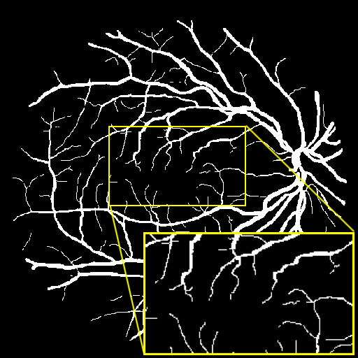
(b) Ground truth

Figure 1: An example of retinal vessels with varying sizes and shapes shown in fundus image and the manually annotated ground truth.

In this paper, we propose an effective and efficient method for accurately segmenting both major and thin vessels in fundus images through learning and decoding hierarchical features with multiple-spatial-frequencies. The main contributions of this work are in three folds:

1. Motivated by the observation that an image of vasculatures can be decomposed into low spatial frequency components that describe the smoothly changing structures such as major vessels and high spatial frequency components that describe the abruptly changing details such as thin vessels, we adopt octave convolution[44] for building feature encoder blocks, and use them to learn hierarchical multifrequency features at multiple levels of a neural network. Moreover, we demonstrate that these low- and high- frequency features learned have different characteristics and can improve the performance of the baseline model with only standard convolutions.

2. For decoding these multifrequency features, we propose a novel operation called octave transposed convolution. This operation takes in feature maps with multiple spatial frequencies and restores the spatial details by learning multiple sets of transposed convolutional kernels. Decoder blocks are built upon these operations, and then utilized for decoding multifrequency feature maps.

3. We also propose a novel encoder-decoder based neural network architecture named Octave UNet, which contains two main components. The encoder utilizes multiple aforementioned multifrequency encoder blocks for hierarchical multifrequency feature learning, whereas the decoder contains multiple aforementioned multifrequency decoder blocks for hierarchical feature decoding. Skip connections similar to those in the standard UNet[33] are also adopted to feed additional location-information-rich feature maps to the decoder blocks to facilitate recovering spatial details and generating the high-resolution probability maps of vessels. The proposed Octave UNet can be trained in an end-to-end manner and deployed to produce vessel segmentation in a single forward feeding without the need of post-processing procedures. Furthermore, the Octave UNet outperforms the baseline UNet in terms of both segmentation performances and computational expenditure, while achieving better or comparable performances to the state-of-the-art methods on four publicly available datasets.

The remaining sections are organized as following: Section II presents the proposed method. Section III introduces the datasets and data augmentation technique used in this work. In Section IV, we present the training methodology and details of implementation, along with comprehensive experimental results. Finally, we conclude this work in Section V.

II Method

II-A Multifrequency feature learning

Retinal vessel forms complex tree-like structure with varying sizes, shapes and vessel widths. As illustrated in Fig.2, the low- and high- frequency components of retinal vasculature focus on capturing major vessels and thin vessels, respectively. Motivated by this observation, we hypothesize that adopting a multi-frequency feature learning approach may be beneficial for segmenting retinal vessels from fundus images. Therefore, the octave convolution[44] is adopted as an extractor for multifrequency features in this work. The computational graph for multifrequency feature transformations of the octave convolution is illustrated in Fig.3. Let $X^{H}$ and $X^{L}$ denote the inputs of high- and low- frequency feature maps, respectively. The high- and low- frequency outputs of the octave convolution are given by $\hat{Y}^{H}=f^{H\rightarrow H}(X^{H})+f^{L\rightarrow H}(X^{L})$ and $\hat{Y}^{L}=f^{L\rightarrow L}(X^{L})+f^{H\rightarrow L}(X^{H})$, where $f^{H\rightarrow H}$ and $f^{L\rightarrow L}$ denote two standard convolution operations for intra-frequency information update, whereas $f^{H\rightarrow L}$ and $f^{L\rightarrow H}$ denote the process of inter-frequency information exchange. Specifically, $f^{H\rightarrow L}$ is equivalent to first downsampling the input by average pooling with a scale of two and then applying a standard convolution for feature transformation, and $f^{L\rightarrow H}$ is equivalent to upsampling the output of a standard convolution by nearest interpolation with a scale of two.

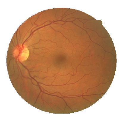
(a) Fundus image

(b) Image of vasculature

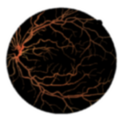
(c) Low frequency component

(d) High frequency component

Figure 2: The image of vasculature can be decomposed into low spatial frequency components that describe the major vascular tree and high spatial frequency components that describe the edges and minor details of thin vessels.

Figure 3: Computation graph of the multifrequency feature transformation of octave convolution. The operation mainly contains two processes of the inter-frequency information exchange ($f^{L\rightarrow H}$ and $f^{H\rightarrow L}$) and intra-frequency information update ($f^{L\rightarrow L}$ and $f^{H\rightarrow H}$).

II-B Decoding multifrequency features

On one hand, during the feature encoding process as shown in Fig.5, while the spatial dimensions of the feature maps reduce gradually, the feature maps lose spatial details step by step. This compression effect forces the kernels to learn more discriminative features with higher levels of abstraction. On the other hand, given only the multifrequency feature extraction is insufficient to perform dense pixel classification for retinal vessel segmentation. A process of decoding feature maps to recover spatial details and generating high resolution probability maps of vessels is needed. One naive way of achieving this is to use bilinear interpolation, which unfortunately lacks the capability of learning the decoding transformation as possessed by the transposed convolution. However, simply using transposed convolutions for multiple layers ignores information exchanges between frequencies within each layer, which may limit the capability of the model to capture more topological relationships and reconstruct segmentation results.

To address these issues, we extend octave convolution and propose a novel operation named octave transposed convolution, which provides the capability of learning suitable mappings for decoding multifrequency features. This operation takes in feature maps with multiple spatial frequencies and restores their spatial details by learning a set of transposed convolution kernels for intra-frequency information update and inter-frequency information exchange.

The multifrequency feature transformation of octave transposed convolution is similar to the transformation of octave convolution as shown in Fig.3. Let $X^{H}$ and $X^{L}$ denote the inputs of high- and low- frequency feature maps, respectively. The high- and low- frequency outputs of the octave transposed convolution are given by $\hat{Y}^{H}=f^{H\rightarrow H}(X^{H})+f^{L\rightarrow H}(X^{L})$ and $\hat{Y}^{L}=f^{L\rightarrow L}(X^{L})+f^{H\rightarrow L}(X^{H})$, where $f^{H\rightarrow H}$ and $f^{L\rightarrow L}$ denote the intra-frequency information update, whereas $f^{H\rightarrow L}$ and $f^{L\rightarrow H}$ denote the inter-frequency information exchange.

Specifically, let $W=\{W^{H\rightarrow H},W^{L\rightarrow L},W^{H\rightarrow L},W^{L\rightarrow H}\}$ denote the octave kernels composed of a set of trainable parameters, $b=\{b^{H\rightarrow H},b^{L\rightarrow L},b^{H\rightarrow L},b^{L\rightarrow H}\}$ denote the biases, $k$ denotes the size of a square kernel, $\sigma(\cdot)$ denotes the non-linear activation function, and $\left\lfloor\cdot\right\rfloor$ denotes the floor operation. The high- and low- frequency responses at location $(i,j)$ of the output are given by (1) and (2), respectively.

$$\hat{Y}^{H}_{(i,j)} {=} \hat{Y}^{L\rightarrow H}_{(i,j)}+\hat{Y}^{H\rightarrow H}_{(i,j)}$$ (1)

$${=} f^{L\rightarrow H}(X^{L})+f^{H\rightarrow H}(X^{H})$$

$${=} \>\sigma(\sum_{m,n}{X^{L}_{(m+\frac{k-1}{2},n+\frac{k-1}{2})}}^{T}W^{L\rightarrow H}_{(\left\lfloor\frac{i}{2}\right\rfloor+m,\left\lfloor\frac{j}{2}\right\rfloor+n)}+b^{L\rightarrow H})$$

$${+}\>\sigma(\sum_{m,n}{X^{H}_{(m+\frac{k-1}{2},n+\frac{k-1}{2})}}^{T}W^{H\rightarrow H}_{(i+m,j+n)}+b^{H\rightarrow H})$$

$$\hat{Y}^{L}_{(i,j)} {=} \hat{Y}^{H\rightarrow L}_{(i,j)}+\hat{Y}^{L\rightarrow L}_{(i,j)}$$ (2)

$${=} f^{H\rightarrow L}(X^{H})+f^{L\rightarrow L}(X^{L})$$

$${=} \>\sigma(\sum_{m,n}{X^{H}_{(m+\frac{k-1}{2},n+\frac{k-1}{2})}}^{T}W^{H\rightarrow L}_{(2i+m+\frac{1}{2},2j+n+\frac{1}{2})}+b^{H\rightarrow L})$$

$${+}\>\sigma(\sum_{m,n}{X^{L}_{(m+\frac{k-1}{2},n+\frac{k-1}{2})}}^{T}W^{L\rightarrow L}_{(i+m,j+n)}+b^{L\rightarrow L})$$

It is worth mentioning that $f^{L\rightarrow L}$ and $f^{H\rightarrow H}$ are standard transposed convolution operations, whereas $f^{H\rightarrow L}$ is equivalent to first downsampling the input by a scale of two (i.e., approximating $X^{H}_{(2i+\frac{1}{2},2j+\frac{1}{2})}$ by using average of all four adjacent locations) and then applying standard transposed convolution. Likewise, $f^{L\rightarrow H}$ is equivalent to upsampling the output of standard transposed convolution by a scale of two, where $X^{L}_{(\left\lfloor\frac{i}{2}\right\rfloor,\left\lfloor\frac{j}{2}\right\rfloor)}$ is implemented with nearest neighbor interpolation.

Moreover, let $\alpha=\frac{c_{\text{low}}}{c_{\text{low}}+c_{\text{high}}}$ denotes the ratio of number of channels of the low-frequency feature maps, where $c_{\text{high}}$ and $c_{\text{low}}$ are the number of channels of high- and low- frequency feature maps, respectively. When $\alpha=0$, the octave transposed convolution outputs only high-frequency feature maps and the computations related to the low-frequency features are ignored. In this case, the octave transposed convolution becomes a standard transposed convolution operation. Without special mentioning, all hyper-parameters $\alpha$ are set to 0.5 in this work.

II-C Octave UNet

In this section, a novel encoder-decoder based neural network architecture named Octave UNet is proposed. After end-to-end training, the proposed Octave UNet is capable of extracting and decoding hierarchical multifrequency features for segmenting retinal vasculature in full-size fundus images. The computation pipeline of the Octave UNet consists of two main processes, i.e., feature encoding and decoding. By utilizing octave convolutions and octave transposed convolutions, we design multifrequency feature encoder blocks and decoder blocks for hierarchical multifrequency feature learning and decoding. By stacking multiple encoder blocks sequentially as shown in Fig.4, hierarchical multifrequency features can learn to capture both the low frequency components that describe the smoothly changing structures such as the major vessels, and high frequency components that describe the abruptly changing details including the fine details of thin vessels, as shown in Fig.5.

According to the feature encoding sequence shown in Fig.4, the feature maps lose spatial details and the precise location information gradually, while the spatial dimensions of the feature maps reduce step by step. An example of this effect is shown in Fig.5. Only using features of high-abstract-level that lack location information is insufficient for generating precise segmentation results. Inspired by the UNet[33], skip connections are adopted to concatenate location-information-rich features to the inputs of decoder blocks as shown in Fig.4. The stacks of decoder blocks in combination with skip connections shown in Fig.4 can facilitate the restoration of location information and spatial details as illustrated in the outputs of decoders in Fig.5.

It is worth mentioning that the initial layer of the Octave UNet shown in Fig.4 contains only computation of $\hat{Y}^{H}=f^{H\rightarrow H}(X^{H})$ and $\hat{Y}^{L}=f^{H\rightarrow L}(X^{H})$, where $X^{H}$ is the input of fundus image and the computation involving $X^{L}$ is ignored. Similarly, the final layer in Fig.4 contains only computation of $\hat{Y}^{H}=f^{H\rightarrow H}(X^{H})+f^{L\rightarrow H}(X^{L})$, where $\hat{Y}^{H}$ is the probability vessel map generated by the Octave UNet and the computation for $\hat{Y}^{L}$ is ignored. For all the trainable kernels within octave convolution and octave transposed convolution layers, the kernel sizes are set to three, while unit strides and one pixel zero paddings at both height and width are adopted. Except for the final layer that is activated by sigmoid function ($\sigma(x)=\frac{1}{1+e^{-x}}$) for performing dense binary classification, ReLU activation ($\sigma(x)=\max(x,0)$) is adopted for all the other layers. Batch normalization[45] is also applied after every layer with trainable parameters. The Octave UNet can be trained in an end-to-end manner on sample pairs of full-size fundus images and vessel ground truths.

Figure 4: Detailed network architecture of the Octave UNet. Feature maps are denoted as cubics with number of channels on the side and spatial dimensions on the top. The spatial dimensions of feature maps remain the same within an encoder or decoder block. An octave convolutions and an octave transposed convolutions are denoted by a blue and green arrow within an octagon, respectively. The red arrows denote max pooling operations that downsample inputs by a scale of two. The gray arrows and plus signs denote skip connections that copy and concatenate feature maps.

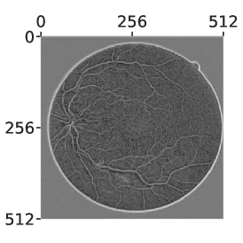
(a) Encoder 0 (high)

(b) Encoder 1 (high)

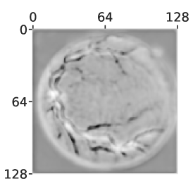
(c) Encoder 2 (high)

(d) Decoder 2 (high)

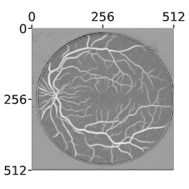
(e) Decoder 1 (high)

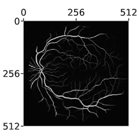
(f) Decoder 0 (high)

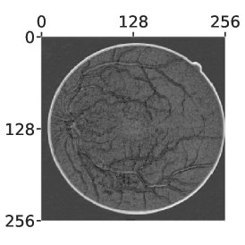
(g) Encoder 0 (low)

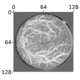
(h) Encoder 1 (low)

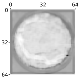
(i) Encoder 2 (low)

(j) Decoder 2 (low)

(k) Decoder 1 (low)

Figure 5: High (first row) and low (second row) frequency kernel responses of encoders and decoders sampled at different abstract level. The first 3 columns show feature maps from different encoders, whereas the last 3 columns show the reconstructed vessel maps from different decoders. The height and width of the feature maps are noted on the axes.

III Datasets

The proposed method is evaluated on four publicly available retinal fundus image datasets: DRIVE[23], STARE[46], CHASE_DB1[47], and HRF[48]. An overview of these four publicly available datasets is provided in Table I.

TABLE I: Overview of datasets adopted in this paper.

Dataset	Year	Description	Resolution
DRIVE	2004	40 in total, 20 for training, 20 for testing.	$565\times 584$
STARE	2000	20 in total, 10 are abnormal.	$700\times 605$
CHASE_DB1	2011	28 in total.	$999\times 960$
HRF	2011	45 in total, 15 each for healthy, diabetic and glaucoma.	$3504\times 2336$

No post-processing steps are needed in the implementation. However, to increase the limited diversity of fundus images, a scheme of data augmentation pipeline is adopted, which mainly includes steps such as horizontal or vertical flipping, adjustment of brightness, saturation or contrast, and gamma adjustment. Each of these steps has a trigger probability of $50\%$.

IV Experiments

IV-A Evaluation metrics

Retinal vessel segmentation is often formulated as a binary dense classification task, i.e., predicting each pixel belonging to positive (vessel) or negative (non-vessel) class within an input image. As shown in Table II, a pixel prediction can fall into one of the four categories, i.e., True Positive (TP), True Negative (TP), False Positive (FP), and False Negative (FN). By plotting these pixels with different color, e.g., TP with Green, FP with Red, TN with Black, and FN with Blue, an analytical vessel map can be generated, as shown in Fig.12.

TABLE II: A binary confusion matrix for vessel segmentation.

Predicted class	Ground truth class
	Vessel	Non-vessel
Vessel	True Positive (TP)	False Negative (FN)
Non-vessel	False Positive (FP)	True Negative (TP)

As listed in Table III, we adopt five commonly used metrics for evaluation: accuracy (ACC), sensitivity (SE), specificity (SP), F1 score (F1), and area under Receiver Operating Characteristic curve (AUROC) for comparison with state-of-the-art methods. In addition, average precision (AP) is adopted to compare the proposed method with the baseline method.

TABLE III: Evaluation metrics adopted in this work.

Evaluation metric	Description
accuracy (ACC)	ACC = (TP + TN) / (TP + TN + FP + FN)
sensitivity (SE)	SE = TP / (TP + FN)
specificity (SP)	SP = TN / (TN + FP)
F1 score (F1)	F1 = (2 * TP) / (2 * TP + FP + FN)
AUROC	Area under the ROC curve.
average precision (AP)	Area under the precision-recall curve.

For methods that use binary thresholding to obtain the final segmentation results, ACC, SE, SP and F1 are dependent on the binarization method. In this paper, without special mentioning, all threshold-sensitive metrics are calculated by global thresholding with threshold $\tau=0.5$. On the other hand, calculating the area under ROC curve requires first creating the ROC curve by plotting the sensitivity against the false positive rate (FPR = FP / (TP + FN)) at various threshold values. Similarly, the average precision is calculated as the area under the precision-recall curve which is plotted by precision (precision = TP / (TP + FP)) against recall (i.e., sensitivity) at various threshold values.

For a model that matches the ground truths perfectly with zero error, its ACC, SE, SP, F1, AUROC and AP should all hit the best score: one.

IV-B Experiment settings

IV-B1 Loss function

To alleviate the effect of imbalanced-classes problem (i.e., the vessel pixel to non-vessel pixel ratio is about $1/9$), class weighted binary cross-entropy as shown in (3) is adopted as the loss function for training, where the positive class weight $w_{pos}=p_{pos}/p_{neg}$ is calculated as the ratio of the positive pixel count $p_{pos}$ to the negative pixel count $p_{neg}$ of the training set. Equation (3) measures the loss of a batch of $m$ samples, in which $y_{n}$ and $\hat{y}_{n}$ denote the ground truth and model prediction of $n\text{-th}$ sample, respectively.

$$L {=} -\sum_{n=1}^{m}{(w_{pos}y_{n}\log{(\hat{y}_{n})}+(1-y_{n})\log{(1-\hat{y}_{n})})}$$ (3)

IV-B2 Training details

All models are trained from scratch with Adam optimizer[49] with default hyper-parameters (e.g., $\beta_{1}=0.9$ and $\beta_{2}=0.999$). The initial learning rate is set to $\eta=0.001$. A shrinking schedule is applied for the current learning rate $\eta_{i}$ as $\eta_{i}=0.9\eta_{i-1}$ after the value of loss function has been saturated for 10 epochs. The training process runs for a total of 1000 epochs to ensure convergence of the model. All trainable kernels are initialized with He initialization[50], and no pre-trained model parameters are used.

IV-B3 Splitting of training and testing set

Except for the DRIVE dataset which has a conventional splitting of training and testing set, the strategy of leave-one-out validation is adopted for STARE, CHASE_DB1, and HRF datasets. Specifically, all images are tested using a model trained on the other images within the same dataset. This strategy for generating training and testing set is also adopted by recent works in[30, 51, 23, 42]. Only the results on test samples are reported.

IV-C Comparison with baseline model

To compare the proposed Octave UNet with the baseline UNet[33], a controlled experiment is conducted, in which all factors are held constant except for the hyper-parameter $\alpha$ that affects the ratio of number of channels of low-frequency features to the total number of channels. (e.g., the baseline UNet has a hyper-parameter of $\alpha=0$). The experimental results of the baseline model and the Octave UNet models with different $\alpha\in[0.25,0.5,0.75]$ are reported in Table IV and presented in Fig.6, which demonstrates that the multi-frequency feature learning indeed improves the performance of the baseline model in terms of all metrics except for specificity, which only reduces very slightly. Furthermore, the performance against computational expenditure curves in Fig.7 shows that the Octave UNet with $\alpha=0.5$ is at a preferable selection, which outperforms the baseline UNet with a reduction of about half of the computational expenditure.

TABLE IV: Performance comparison of the baseline UNet and the Octave UNets on the DRIVE dataset.

Model	# Parameter (M)	FLOPs (G)	ACC	SE	SP	F1	AUROC	AP
baseline UNet ($\alpha=0$)	16.53	133.93	0.9616	0.7768	0.9796	0.7795	0.9543	0.8238
Octave UNet ($\alpha=0.25$)	16.54	90.25	0.9659	0.8483	0.9775	0.8126	0.9849	0.9042
Octave UNet ($\alpha=0.5$)	16.54	58.88	0.9663	0.8375	0.9790	0.8127	0.9835	0.9027
Octave UNet ($\alpha=0.75$)	16.54	39.97	0.9628	0.8465	0.9742	0.7985	0.9803	0.8913

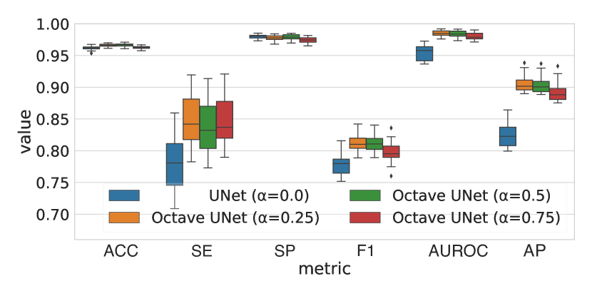
Figure 6: Box plot comparing the baseline UNet and the Octave UNets on the DRIVE dataset.

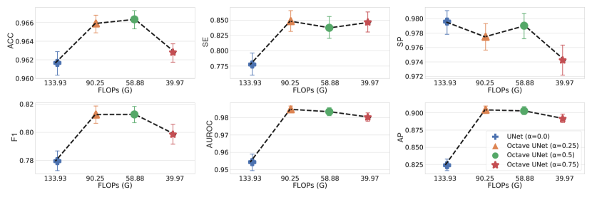
Figure 7: Comparison of performance and computational expenditure of the baseline UNet and the Octave UNets on the DRIVE dataset.

An example of the probability maps generated by the baseline UNet and the Octave UNet are presented in Fig.8, which shows that the Octave UNet can better capture the fine details of thin vessels and segment the major vessels with better connectivity than the baseline UNet.

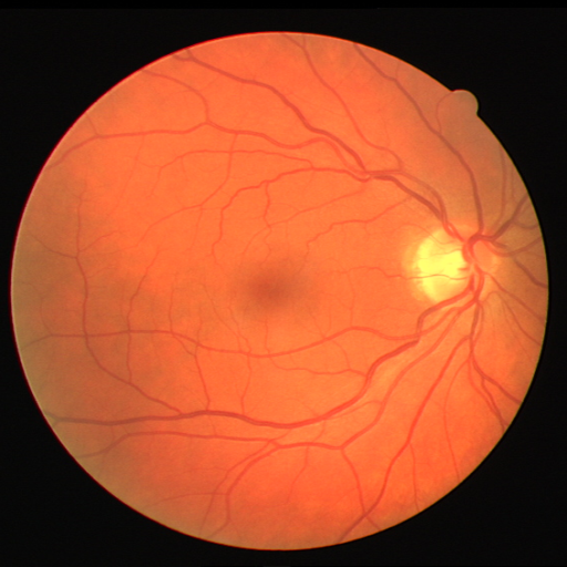
(a) Fundus image

(b) Ground truth

(c) Probability map of the baseline UNet

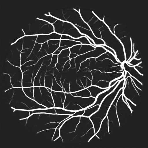
(d) Probability map of the Octave UNet

Figure 8: An example in the DRIVE dataset, with (a) the original fundus image, (b) the corresponding ground truth, (c) the probability map generated by the baseline UNet, and (d) the probability map generated by the Octave UNet. The Octave UNet shows better performance in capturing the thin vessels while having better connectivity.

Moreover, a frequency analysis of the feature maps learned by the Octave UNet and the baseline UNet is conducted and the results are presented in Fig.9. Specifically, the feature maps generated by the intermediate encoders and decoders of the Octave UNet and the baseline UNet are first obtained by feeding both the models with the same fundus images in DRIVE dataset. Then the two dimensional Fast Fourier Transformation (FFT) is applied on each feature map to obtain the energy map of frequencies, followed by shifting the low frequency components of the energy map to the center while the high frequency components to the edges. Finally, the two dimensional energy maps of shifted FFT response generated from the baseline UNet, the high frequency group of the Octave UNet and the low frequency group of the Octave UNet are respectively averaged to generate the final results shown in (a), (b), and (c) of Fig.9. Furthermore, to make it easier to distinguish the difference, the final results of two dimensional energy maps are transformed into one dimensional signals as shown in (d) of Fig.9 by first averaging pixels representing the same frequencies and then sorting the averaged pixel values according to the frequencies their represents.

It can be observed that the features learned by the Octave UNet obtain different frequency characteristics than those of the baseline UNet. Specifically, the energy of the low frequency group of the Octave UNet is more focused around the zero frequency than those of the high frequency group, whereas the energy of the high frequency group of the Octave UNet contains more high frequency components than the those of the baseline UNet. Combining with the experimental results, this observation supports the hypothesis that adopting multi-frequency feature learning indeed improves the performance of segmenting retinal vessels with varying sizes and shapes.

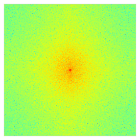
(a) baseline UNet

(b) Octave UNet (high)

(c) Octave UNet (low)

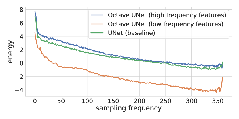
(d) Frequency spectrums

Figure 9: Frequency analysis of feature maps. The two dimensional energy maps (a), (b) and (c) are the responses of Fourier transformation of feature maps obtained from the baseline UNet, high frequency features of the Octave UNet and low frequency features of the Octave UNet, respectively. The one dimensional spectrum curves in (d) are generated from the two dimensional energy maps, respectively.

IV-D Comparison with other state-of-the-art methods

The performance comparison of the proposed method and the state-of-the-art methods are reported in Table V, Table VI, Table VII, and Table VII for DRIVE, STARE, CHASE_DB1, and HRF dataset, respectively. The proposed method outperforms all the other state-of-the-art methods in terms of ACC, SE, and F1 on all datasets. Specifically, the proposed method achieves the best performance in all metrics on CHASE_DB1 and HRF datasets. For DRIVE dataset, the proposed method achieves best ACC, SE, F1, and AUROC, while its SP is slightly lower than the patch based R2-UNet[35]. For STARE dataset, the proposed Octave UNet obtains metrics of SP and AUROC comparable to the two patch based methods: DeepVessel[51] and R2-UNet[35], while achieving best performance on all the other metrics. Overall, the proposed method achieves better or comparable performance against the other state-of-the-art methods.

TABLE V: Comparison with other state-of-the-art methods on the DRIVE dataset.

Methods	Year	ACC	SE	SP	F1	AUROC
Unsupervised Methods
Zena and Klein[10]	2001	0.9377	0.6971	0.9769	N/A	0.8984
Mendonca and Campilho[11]	2006	0.9452	0.7344	0.9764	N/A	N/A
Al-Diri et al.[20]	2009	0.9258	0.7282	0.9551	N/A	N/A
Miri and Mahloojifar[12]	2010	0.9458	0.7352	0.9795	N/A	N/A
You et al.[15]	2011	0.9434	0.7410	0.9751	N/A	N/A
Fraz et al.[52]	2012	0.9430	0.7152	0.9768	N/A	N/A
Fathi et al.[53]	2013	N/A	0.7768	0.9759	0.7669	N/A
Roychowdhury et al.[54]	2015	0.9494	0.7395	0.9782	N/A	N/A
Fan et al.[13]	2019	0.9600	0.7360	0.9810	N/A	N/A
Supervised Methods
Staal et al.[23]	2004	0.9441	0.7194	0.9773	N/A	0.9520
Marin et al.[6]	2011	0.9452	0.7067	0.9801	N/A	0.9588
Fraz et al.[47]	2012	0.9480	0.7460	0.9807	N/A	0.9747
Cheng et al.[55]	2014	0.9472	0.7252	0.9778	N/A	0.9648
Vega et al.[56]	2015	0.9412	0.7444	0.9612	0.6884	N/A
Antiga[34]	2016	0.9548	0.7642	0.9826	0.8115	0.9775
Fan et al.[28]	2016	0.9614	0.7191	0.9849	N/A	N/A
Fan and Mo[27]	2016	0.9612	0.7814	0.9788	N/A	N/A
Liskowski et al.[51]	2016	0.9535	0.7811	0.9807	N/A	0.9790
Li et al.[30]	2016	0.9527	0.7569	0.9816	N/A	0.9738
Orlando et al.[57]	2017	N/A	0.7897	0.9684	0.7857	N/A
Mo and Zhang[42]	2017	0.9521	0.7779	0.9780	N/A	0.9782
Xiao et al.[58]	2018	0.9655	0.7715	N/A	N/A	N/A
Alom et al.[35]	2019	0.9556	0.7792	0.9813	0.8117	0.9784
Lei et al.[43]	2019	0.9607	0.8132	0.9783	N/A	0.9796
The Proposed Method	2020	0.9664	0.8374	0.9790	0.8127	0.9835

TABLE VI: Comparison with other state-of-the-art methods on the STARE dataset

Methods	Year	ACC	SE	SP	F1	AUROC
Unsupervised Methods
Mendonca and Campilho[11]	2006	0.9440	0.6996	0.9730	N/A	N/A
Al-Diri et al.[20]	2009	N/A	0.7521	0.9681	N/A	N/A
You et al.[15]	2011	0.9497	0.7260	0.9756	N/A	N/A
Fraz et al.[52]	2012	0.9442	0.7311	0.9680	N/A	N/A
Fathi et al.[53]	2013	N/A	0.8061	0.9717	0.7509	N/A
Roychowdhury et al.[54]	2015	0.9560	0.7317	0.9842	N/A	N/A
Fan et al.[13]	2019	0.9570	0.7910	0.9700	N/A	N/A
Supervised Methods
Staal et al.[23]	2004	0.9516	N/A	N/A	N/A	0.9614
Marin et al.[6]	2011	0.9526	0.6944	0.9819	N/A	0.9769
Fraz et al.[52]	2012	0.9534	0.7548	0.9763	N/A	0.9768
Vega et al.[56]	2015	0.9483	0.7019	0.9671	0.6614	N/A
Fan et al.[28]	2016	0.9588	0.6996	0.9787	N/A	N/A
Fan and Mo[27]	2016	0.9654	0.7834	0.9799	N/A	N/A
Liskowski et al.[51]	2016	0.9729	0.8554	0.9862	N/A	0.9928
Li et al.[30]	2016	0.9628	0.7726	0.9844	N/A	0.9879
Orlando et al.[57]	2017	N/A	0.7680	0.9738	0.7644	N/A
Mo and Zhang[42]	2017	0.9674	0.8147	0.9844	N/A	0.9885
Xiao et al.[58]	2018	0.9693	0.7469	N/A	N/A	N/A
Alom et al.[35]	2019	0.9712	0.8292	0.9862	0.8475	0.9914
Lei et al.[43]	2019	0.9698	0.8398	0.9761	N/A	0.9858
The Proposed Method	2020	0.9713	0.8664	0.9798	0.8191	0.9875

TABLE VII: Comparison with other state-of-the-art methods on the CHASE_DB1 dataset

Methods	Year	ACC	SE	SP	F1	AUROC
Unsupervised Methods
Fraz et al.[52]	2012	0.9469	0.7224	0.9711	N/A	0.9712
Roychowdhury et al.[54]	2015	0.9467	0.7615	0.9575	N/A	N/A
Fan et al.[13]	2019	0.9510	0.6570	0.9730	N/A	N/A
Supervised Methods
Fraz et al.[59]	2014	N/A	0.7259	0.9770	0.7488	N/A
Fan and Mo[27]	2016	0.9573	0.7656	0.9704	N/A	N/A
Liskowski et al.[51]	2016	0.9628	0.7816	0.9836	N/A	0.9823
Li et al.[30]	2016	0.9527	0.7569	0.9816	N/A	0.9738
Orlando et al.[57]	2017	N/A	0.7277	0.9712	0.7332	N/A
Mo and Zhang[42]	2017	0.9581	0.7661	0.9793	N/A	0.9812
Alom et al.[35]	2019	0.9634	0.7756	0.9820	0.7928	0.9815
Lei et al.[43]	2019	0.9648	0.8275	0.9768	N/A	0.9812
The Proposed Method	2020	0.9759	0.8670	0.9840	0.8313	0.9905

TABLE VIII: Comparison with other state-of-the-art methods on the HRF dataset

Methods	Year	ACC	SE	SP	F1	AUROC
Unsupervised Methods
Roychowdhury et al.[54]	2015	0.9467	0.7615	0.9575	N/A	N/A
Supervised Methods
Kolar et al.[48]	2013	N/A	0.7794	0.9584	0.7158	N/A
Orlando et al.[57]	2017	N/A	0.7874	0.9584	0.7158	N/A
The Proposed Method	2020	0.9698	0.8076	0.9831	0.7963	0.9845

The computation time needed for processing a fundus image in the DRIVE dataset using the proposed method is also compared with other state-of-the-art methods that use patch based or end-to-end approaches and the results are shown in Table IX. Without the need of cropping and merging patches as in the patch based UNet[34], the end-to-end approaches are typically faster. Without the need of pre- and post- processing, the proposed method can generate high resolution vessel segmentation in a single forward feeding of a full-sized fundus image in the DRIVE dataset in about $0.4s$.

TABLE IX: Computation time comparison with other state-of-the-art methods on a fundus image in the DRIVE dataset.

Methods	Year	Main device	Computation time
Antiga[34] (patch based UNet)	2016	NVIDIA GTX Titan Xp	10.5 s
Mo and Zhang[42] (end-to-end FCN)	2017	NVIDIA GTX Titan Xp	0.4 s
Fan et al.[13] (unsupervised image matting)	2019	NVIDIA GTX Titan Xp	6.2 s
Alom et al.[35] (patch based recurrent UNet)	2019	NVIDIA GTX Titan Xp	2.8 s
The baseline UNet	2020	Intel Xeon CPU @ 2.40GHz	4.5 s
The Proposed Method	2020	Intel Xeon CPU @ 2.40GHz	3.0 s
		NVIDIA GTX Titan Xp	0.4 s

IV-E Sensitivity analysis of global threshold

The threshold-sensitive metrics: ACC, SE, SP, and F1 are measured at various global threshold values sampled in $\tau_{i}\in 0.01,\dots,0.99$. The resulting sensitivity curves are shown in Fig.10. The sensitivity curves of the proposed method have similar profiles on all datasets tested, which demonstrates the robustness of the proposed Octave UNet across different datasets. Furthermore, near the adopted threshold, i.e., $\tau=0.5$, the sensitivity curves of ACC, SP, and F1 change very slightly, which further demonstrates the robustness of the proposed method against the global threshold. Moreover, by lowering the threshold $\tau$ to about 0.25, the proposed method can achieve significant gain on SE, while the other metrics decrease very slightly.

Figure 10: Sensitivity curves of the proposed method on different datasets.

IV-F Performance on abnormal cases

The vessel segmentation results of the proposed method on cases with abnormalities are shown in Fig.11, which demonstrates the robust performance of the proposed method against various abnormalities such as exudates, cotton wool spots, hemorrhages, and pathological lesions.

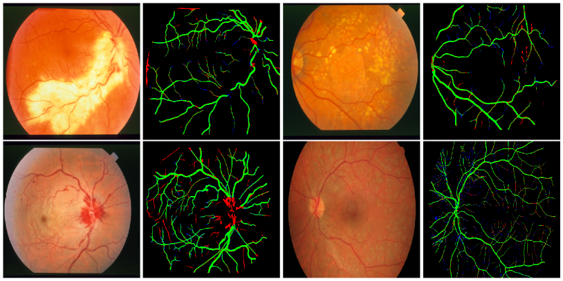
Figure 11: The original fundus images and the analytical vessel segmentation results of cases with exudates, cotton wool spots, hemorrhages, and lesions, respectively. The proposed method can segment retinal vasculatures with different types of abnormal regions in fundus images. The analytic results (as shown in the second and last columns) are plotted by painting TP with green pixels, FP with red pixels, FN with blue pixels, and TN with black pixels.

The best and worst performances on different datasets are illustrated in Fig.12. The best cases on all datasets contain very few missed thin vessels. On the other hand, the worst cases show that the proposed method are affected by uneven illuminations. In both best and worst cases, the proposed method is capable of discriminatively separating non-vascular structures and vasculatures.

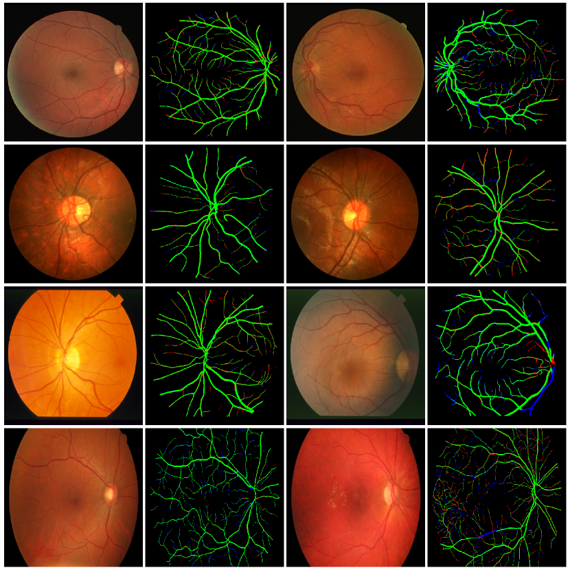
Figure 12: The best (first 2 columns) and worst (last 2 columns) cases on DRIVE (first row), STARE (second row), CHASE_DB1 (third row) and HRF (last row) datasets. The analytic results (second and last columns) are obtained by plotting TP with green, FP with read, FN with blue, and TN with black.

V Conclusion

An effective and efficient method for retinal vessel segmentation based on multifrequency convolutional network is proposed in this paper. Built upon octave convolution and the proposed octave transposed convolution, the carefully designed Octave UNet can extract hierarchical features with multiple-spatial-frequencies and reconstruct accurate vessel segmentation maps. Benefiting from the design of hierarchical multifrequency features, the Octave UNet outperforms the baseline model in terms of both segmentation performances and computational expenditure. Comprehensive experimental results also demonstrate that the Octave UNet achieves better or comparable performances against the other state-of-the-art methods.

References

- [1] C. L. Srinidhi, P. Aparna, and J. Rajan, “Recent advancements in retinal vessel segmentation,” J. Med. Syst., vol. 41, no. 4, pp. 70–99, Apr. 2017.
- [2] M. M. Fraz, P. Remagnino, A. Hoppe, B. Uyyanonvara, A. R. Rudnicka, C. G. Owen et al., “Blood vessel segmentation methodologies in retinal images - a survey,” Comput. Methods Prog. Biomed., vol. 108, no. 1, pp. 407–433, Oct. 2012.
- [3] P. Vostatek, E. Claridge, H. Uusitalo, M. Hauta-Kasari, P. Falt, and L. Lensu, “Performance comparison of publicly available retinal blood vessel segmentation methods,” Comput. Med. Imag. Grap., vol. 55, pp. 2–12, Jan. 2017.
- [4] C. Heneghan, J. Flynn, M. O’Keefe, and M. Cahill, “Characterization of changes in blood vessel width and tortuosity in retinopathy of prematurity using image analysis,” Med. Image Anal., vol. 6, no. 4, pp. 407–429, Dec. 2002.
- [5] R. A. Welikala, J. Dehmeshki, A. Hoppe, V. Tah, S. Mann, T. H. Williamson et al., “Automated detection of proliferative diabetic retinopathy using a modified line operator and dual classification,” Comput. Methods Prog. Biomed., vol. 114, no. 3, pp. 247–261, May 2014.
- [6] C. Marino, M. G. Penedo, M. Penas, M. J. Carreira, and F. Gonzalez, “Personal authentication using digital retinal images,” Pattern Anal. Appl., vol. 9, no. 1, pp. 21–33, Jan. 2006.
- [7] C. Kose and C. Ikibaşs, “A personal identification system using retinal vasculature in retinal fundus images,” Expert Syst. Appl., vol. 38, no. 11, pp. 13 670–13 681, Oct. 2011.
- [8] T. A. Soomro, A. J. Afifi, L. Zheng, S. Soomro, J. Gao, O. Hellwich et al., “Deep learning models for retinal blood vessels segmentation: a review,” IEEE Access, vol. 7, pp. 71 696–71 717, June 2019.
- [9] S. Moccia, E. D. Momi, S. E. Hadji, and L. S. Mattos, “Blood vessel segmentation algorithms — review of methods, datasets and evaluation metrics,” Comput. Methods Prog. Biomed., vol. 158, pp. 71–91, May 2018.
- [10] F. Zana and J. C. Klein, “Segmentation of vessel-like patterns using mathematical morphology and curvature evaluation,” IEEE Trans. Image Process., vol. 10, no. 7, pp. 1010–1019, July 2001.
- [11] A. M. Mendonca and A. Campilho, “Segmentation of retinal blood vessels by combining the detection of centerlines and morphological reconstruction,” IEEE Trans. Med. Imag., vol. 25, no. 9, pp. 1200–1213, Sept. 2006.
- [12] M. S. Miri and A. Mahloojifar, “Retinal image analysis using curvelet transform and multistructure elements morphology by reconstruction,” IEEE Trans. Biomed. Eng., vol. 58, no. 5, pp. 1183–1192, May 2010.
- [13] Z. Fan, J. Lu, C. Wei, H. Huang, X. Cai, and X. Chen, “A hierarchical image matting model for blood vessel segmentation in fundus images,” IEEE Trans. Image Process., vol. 28, no. 5, pp. 2367–2377, Dec. 2019.
- [14] S. Chaudhuri, S. Chatterjee, N. Katz, M. Nelson, and M. Goldbaum, “Detection of blood vessels in retinal images using two-dimensional matched filters,” IEEE Trans. Med. Imag., vol. 8, no. 3, pp. 263–269, Sept. 1989.
- [15] X. You, Q. Peng, Y. Yuan, Y.-m. Cheung, and J. Lei, “Segmentation of retinal blood vessels using the radial projection and semi-supervised approach,” Pattern Recognit., vol. 44, no. 10-11, pp. 2314–2324, Oct. 2011.
- [16] Y. Wang, G. Ji, P. Lin, and E. Trucco, “Retinal vessel segmentation using multiwavelet kernels and multiscale hierarchical decomposition,” Pattern Recognit., vol. 46, no. 8, pp. 2117–2133, Aug. 2013.
- [17] J. Zhang, B. Dashtbozorg, E. Bekkers, J. P. W. Pluim, R. Duits, and B. M. ter Haar Romeny, “Robust retinal vessel segmentation via locally adaptive derivative frames in orientation scores,” IEEE Trans. Med. Imag., vol. 35, no. 12, pp. 2631–2644, Dec. 2016.
- [18] E. Ricci and R. Perfetti, “Retinal blood vessel segmentation using line operators and support vector classification,” IEEE Trans. Med. Imag., vol. 26, no. 10, pp. 1357–1365, Oct. 2007.
- [19] U. T. Nguyen, A. Bhuiyan, L. A. Park, and K. Ramamohanarao, “An effective retinal blood vessel segmentation method using multi-scale line detection,” Pattern Recognit., vol. 46, no. 3, pp. 703–715, Mar. 2013.
- [20] B. Al-Diri, A. Hunter, and D. Steel, “An active contour model for segmenting and measuring retinal vessels,” IEEE Trans. Med. Imag., vol. 28, no. 9, pp. 1488–1497, Sept. 2009.
- [21] I. Liu and Y. Sun, “Recursive tracking of vascular networks in angiograms based on the detection-deletion scheme,” IEEE Trans. Med. Imag., vol. 12, no. 2, pp. 334–341, June 1993.
- [22] Y. Yin, M. Adel, and S. Bourennane, “Retinal vessel segmentation using a probabilistic tracking method,” Pattern Recognit., vol. 45, no. 4, pp. 1235–1244, Apr. 2012.
- [23] J. Staal, M. D. Abramoff, M. Niemeijer, M. A. Viergever, and B. Van Ginneken, “Ridge-based vessel segmentation in color images of the retina,” IEEE Trans. Med. Imag., vol. 23, no. 4, pp. 501–509, Apr. 2004.
- [24] J. V. B. Soares, J. J. G. Leandro, R. M. Cesar, H. F. Jelinek, and M. J. Cree, “Retinal vessel segmentation using the 2d gabor wavelet and supervised classification,” IEEE Trans. Med. Imag., vol. 25, no. 9, pp. 1214–1222, Sept. 2006.
- [25] D. Marin, A. Aquino, M. E. Gegundez-Arias, J. M. Bravo, D. Marin, A. Aquino et al., “A new supervised method for blood vessel segmentation in retinal images by using gray-level and moment invariants-based features,” IEEE Trans. Med. Imag., vol. 30, no. 1, pp. 146–158, Jan. 2011.
- [26] A. Fathi and A. R. Naghsh-Nilchi, “General rotation-invariant local binary patterns operator with application to blood vessel detection in retinal images,” Pattern Anal. Appl., vol. 17, no. 1, pp. 69–81, Feb. 2014.
- [27] Z. Fan and J. Mo, “Automated blood vessel segmentation based on de-noising auto-encoder and neural network,” in Proc. Int. Conf. Mach. Learn. and Cybern. (ICMLC), vol. 2. IEEE, July 2016, pp. 849–856.
- [28] Z. Fan, Y. Rong, J. Lu, J. Mo, F. Li, X. Cai et al., “Automated blood vessel segmentation in fundus image based on integral channel features and random forests,” in Proc. 12th World Congr. Int. Control and Autom. (WCICA). IEEE, Sept. 2016, pp. 2063–2068.
- [29] J. Zhang, Y. Chen, E. Bekkers, M. Wang, B. Dashtbozorg, and B. M. ter Haar Romeny, “Retinal vessel delineation using a brain-inspired wavelet transform and random forest,” Pattern Recognit., vol. 69, pp. 107–123, Sept. 2017.
- [30] Q. Li, B. Feng, L. Xie, P. Liang, H. Zhang, and T. Wang, “A cross-modality learning approach for vessel segmentation in retinal images,” IEEE Trans. Med. Imag., vol. 35, no. 1, pp. 109–118, Jan. 2016.
- [31] A. Oliveira, S. Pereira, and C. A. Silva, “Retinal vessel segmentation based on fully convolutional neural networks,” Expert Syst. Appl., vol. 112, pp. 229–242, Dec. 2018.
- [32] E. Shelhamer, J. Long, and T. Darrell, “Fully convolutional networks for semantic segmentation,” IEEE Trans. Pattern Anal. Mach. Intell., vol. 39, no. 4, pp. 640–651, Apr. 2017.
- [33] O. Ronneberger, P. Fischer, and T. Brox, “U-net: convolutional networks for biomedical image segmentation,” in Int. Conf. Med. Image Comput. and Computer-Assisted Intervention (MICCAI), vol. 9351. Springer, Nov. 2015, pp. 234–241.
- [34] L. Antiga, “Retina blood vessel segmentation with a convolutional neural network,” 2016. [Online]. Available: https://github.com/orobix/retina-unet
- [35] M. Z. Alom, C. Yakopcic, M. Hasan, T. M. Taha, and V. K. Asari, “Recurrent residual u-net for medical image segmentation,” J. Med. Imag., vol. 6, no. 1, pp. 1–16, Jan. 2019.
- [36] K. He, X. Zhang, S. Ren, and J. Sun, “Deep residual learning for image recognition,” in Proc. IEEE Conf. Comput. Vis. and Pattern Recognit. (CVPR), Dec. 2016, pp. 770–778.
- [37] M. Liang and X. Hu, “Recurrent convolutional neural network for object recognition,” in Proc. IEEE Conf. Comput. Vis. and Pattern Recognit. (CVPR), June 2015, pp. 3367–3375.
- [38] H. Fu, Y. Xu, S. Lin, D. W. Kee Wong, and J. Liu, “Deepvessel: retinal vessel segmentation via deep learning and conditional random field,” in Int. Conf. Med. Image Comput. and Computer-Assisted Intervention (MICCAI). Springer, Oct. 2016, pp. 132–139.
- [39] H. Fu, Y. Xu, D. W. K. Wong, and J. Liu, “Retinal vessel segmentation via deep learning network and fully-connected conditional random fields,” in Proc. IEEE 13th Int. Symp. Biomed. Imag. (ISBI), Apr. 2016, pp. 698–701.
- [40] C.-Y. Lee, S. Xie, P. Gallagher, Z. Zhang, and Z. Tu, “Deeply-supervised nets,” in Proc. 8th Int. Conf. Artif. Intell. and Stat., vol. 38. PRML, May 2015, pp. 562–570.
- [41] S. Zheng, S. Jayasumana, B. Romera-Paredes, V. Vineet, Z. Su, D. Du et al., “Conditional random fields as recurrent neural networks,” in Proc. IEEE Int. Conf. Comput. Vis. (ICCV), Dec. 2015, pp. 1529–1537.
- [42] J. Mo and L. Zhang, “Multi-level deep supervised networks for retinal vessel segmentation,” Int. J. Comput. Ass. Rad., vol. 12, no. 12, pp. 2181–2193, Dec. 2017.
- [43] M. Lei, C. Li, C. Jun, G. Zaiwang, Z. Yitian, and L. Jiang, “Dense dilated network with probability regularized walk for vessel detection,” IEEE Trans. Med. Imag., vol. 39, no. 5, pp. 1392–1403, Oct. 2019.
- [44] Y. Chen, H. Fang, B. Xu, Z. Yan, Y. Kalantidis, M. Rohrbach et al., “Drop an octave: reducing spatial redundancy in convolutional neural networks with octave convolution,” in Proc. IEEE Int. Conf. Comput. Vis. (ICCV), vol. 1, Apr. 2019, pp. 3434–3443.
- [45] S. Ioffe and C. Szegedy, “Batch normalization: accelerating deep network training by reducing internal covariate shift,” in Proc. 32nd Int. Conf. on Mach. Learn. (ICML), vol. 37, July 2015, pp. 448–456.
- [46] A. D. Hoover, V. Kouznetsova, and M. Goldbaum, “Locating blood vessels in retinal images by piecewise threshold probing of a matched filter response,” IEEE Trans. Med. Imag., vol. 19, no. 3, pp. 203–210, Mar. 2000.
- [47] M. M. Fraz, P. Remagnino, A. Hoppe, B. Uyyanonvara, A. R. Rudnicka, C. G. Owen et al., “An ensemble classification-based approach applied to retinal blood vessel segmentation,” IEEE Trans. Biomed. Eng., vol. 59, no. 9, pp. 2538–2548, Sept. 2012.
- [48] J. Odstrcilik, R. Kolar, T. Kubena, P. Cernosek, A. Budai, J. Hornegger et al., “Retinal vessel segmentation by improved matched filtering: evaluation on a new high-resolution fundus image database,” IET Image Process., vol. 7, no. 4, pp. 373–383, June 2013.
- [49] D. P. Kingma and J. Ba, “Adam: a method for stochastic optimization,” in Proc. 3rd Int. Conf. Learn. Repr. (ICLR), Dec. 2015.
- [50] K. He, X. Zhang, S. Ren, and J. Sun, “Delving deep into rectifiers: Surpassing human-level performance on imagenet classification,” in Proc. IEEE Int. Conf. Comput. Vis. (ICCV), Dec. 2015, pp. 1026–1034.
- [51] P. Liskowski and K. Krawiec, “Segmenting retinal blood vessels with deep neural networks.” IEEE Trans. Med. Imag., vol. 35, no. 11, pp. 2369–2380, Nov. 2016.
- [52] M. M. Fraz, S. A. Barman, P. Remagnino, A. Hoppe, A. Basit, B. Uyyanonvara et al., “An approach to localize the retinal blood vessels using bit planes and centerline detection,” Comput. Methods Prog. Biomed., vol. 108, no. 2, pp. 600–616, Nov. 2012.
- [53] A. Fathi and A. R. Naghsh-Nilchi, “Automatic wavelet-based retinal blood vessels segmentation and vessel diameter estimation,” Biomedical Signal Processing and Control, vol. 8, no. 1, pp. 71–80, 2013.
- [54] S. Roychowdhury, D. D. Koozekanani, and K. K. Parhi, “Iterative vessel segmentation of fundus images,” IEEE Trans. Biomed. Eng., vol. 62, no. 7, pp. 1738–1749, Feb. 2015.
- [55] E. Cheng, L. Du, Y. Wu, Y. J. Zhu, V. Megalooikonomou, and H. Ling, “Discriminative vessel segmentation in retinal images by fusing context-aware hybrid features,” Mach. Vis. Appl., vol. 25, no. 7, pp. 1779–1792, Oct. 2014.
- [56] R. Vega, G. Sanchez-Ante, L. E. Falcon-Morales, H. Sossa, and E. Guevara, “Retinal vessel extraction using lattice neural networks with dendritic processing,” Comput. Biol. Med., vol. 58, pp. 20–30, Mar. 2015.
- [57] J. I. Orlando, E. Prokofyeva, and M. B. Blaschko, “A discriminatively trained fully connected conditional random field model for blood vessel segmentation in fundus images,” IEEE Trans. Biomed. Eng., vol. 64, no. 1, pp. 16–27, Jan. 2017.
- [58] X. Xiao, S. Lian, Z. Luo, and S. Li, “Weighted res-unet for high-quality retina vessel segmentation,” in Proc. 9th Int. Conf. Inf. Technol. Med. and Educ. (ITME), Oct. 2018, pp. 327–331.
- [59] M. M. Fraz, A. R. Rudnicka, C. G. Owen, and S. A. Barman, “Delineation of blood vessels in pediatric retinal images using decision trees-based ensemble classification,” Int. J. Comput. Ass. Rad., vol. 9, no. 5, pp. 795–811, Sept. 2014.