Neutrino decoherence in presence of strong gravitational fields

Abstract

We explore the impact of strong gravitational fields on neutrino decoherence. To this aim, we employ the density matrix formalism to describe the propagation of neutrino wave packets in curved spacetime. By considering Gaussian wave packets, we determine the coherence proper time, neglecting the effect of matter outside the compact object. We show that strong gravitational fields nearby compact objects significantly influence neutrino coherence.

1 Introduction

Neutrinos are elementary massive particles with non-zero mixings producing neutrino oscillations, a quantum mechanical phenomenon analogous to Rabi oscillations in atomic physics [1, 2]. This phenomenon depends on the fact that the flavor and the mass basis are related by the Pontecorvo-Maki-Nakagawa-Sakata unitary matrix (PMNS) whose mixing angles are known. As for the Dirac CP violating phase, there are indications for it to be large [3], while Majorana phases remain unknown. Neutrino masses require extensions of the Glashow-Weinberg-Salam Model as e.g. including three right handed singlets and Yukawa couplings.

Neutrino oscillation studies typically employ the plane wave approximation to describe flavor conversion. Wave packets (WPs) account for neutrinos being localized particles. Their use introduces decoherence among the mass eigenstates due to the finite extension of corresponding WPs [4]. In laboratory experiments, the WP widths include the finite size both at neutrino production and at detection. In the WP treatment an exponential factor suppresses coherence in the interference term of the oscillation probabilities. However, at typical distances of oscillation experiments, this correction is negligeable [5, 6, 7]. Besides WP separation, other mechanisms produce neutrino decoherence, such as the propagation in a quantum gravity foam [8], for which experimental constraints exist (see e.g. [9]).

In matter the WP widths associated with neutrino production processes (such as inverse beta-decay) are small, around $10^{-11}-10^{-12}~{}$cm [10, 11]. In dense environments the WP treatment has implications depending on the adiabaticity. In case of adiabatic evolution, a WP description in the matter basis introduces an exponential suppression factor with a coherence length that is similar to the vacuum case [10, 11]. On the other hand, if neutrino evolution is non-adiabatic, mass eigenstate mixing is not suppressed which makes difficult to even define a coherence length. Consequently decoherence by WP separation depends on the model chosen for adiabaticity violation [11].

So far, investigations of neutrino flavor conversion based on WPs have been performed in flat spacetime. Nearby a neutron star or a black hole, strong gravitational fields influence neutrino flavor evolution. Effects due to trajectory bending on nucleosynthetic outcomes have been studied in a black hole accretion disk [12], while Ref. [13] has presented a general relativistic ray tracing for neutrinos. Neutrino trajectories in the Schwarzschild metric are explored in [14]. Ref.[15] presents the neutrino dynamics and the influence on the electron fraction of a slowly rotating nonlinear charged black hole. In dense environments, gravitational fields can also modify the localization and adiabaticity of the Mikheev-Smirnov-Wolfenstein resonance [16], or delay bipolar oscillations from neutrino self-interactions [17]. Such studies are based on the plane wave approximation.

In this letter we explore the impact of strong gravitational fields on neutrino decoherence in a WP treatment. We first recall the density matrix formalism using WPs in the case of flat spacetime. Then we extend it to describe neutrino flavor evolution in curved spacetime, considering a static and spherically symmetric gravitational field described by the Schwarzschild metric. Neutrino decoherence in curved spacetime is quantified by a coherence proper time, instead of a coherence proper length, as in flat spacetime. We first introduce kinematical arguments and then derive the neutrino coherence proper time based on density matrices with Gaussian WPs. We neglect matter and neutrino self-interactions outside the compact object. Finally, we present numerical estimates of the gravitational field effects on the coherence proper time.

This letter is structured as follows. Section II recalls the WP treatment of neutrino oscillations in vacuum and introduces the coherence length in flat spacetime. Section III presents the extension of the formalism to curved spacetime in the Schwarzschild metric. Then kinematical arguments are presented and the derivation of the coherence proper time based on the density matrix formalism for WPs. Numerical results for the coherence proper time are shown. Section IV gives our conclusions.

2 Neutrino WP decoherence in flat spacetime

2.1 Neutrino states

A neutrino state in coordinate space can be Fourier expanded as (we take $\hbar=c=G=1$) [11]

$$|\nu(t,\vec{x})\rangle=\int_{\vec{p}}e^{i\vec{p}\cdot\vec{x}}|\nu(t,\vec{p})\rangle,$$ (1)

with $|\nu(t,\vec{p})\rangle$ the time-dependent state with momentum $\vec{p}$. A vector of N such states, $N$ being the number of neutrino families, is solution of the Schrödinger-like equation

$$i{{\rm d}\over{\rm dt}}|\nu(t,\vec{p})\rangle=h(t,\vec{p})~{}|\nu(t,\vec{p})\rangle,$$ (2)

where $h(t,\vec{p})$ is the Hamiltonian governing neutrino evolution. In astrophysical environments, it includes different contributions

$$h(t,\vec{p})=h_{\text{vac}}(\vec{p})+h_{mat}(t)+h_{\nu\nu}(t),$$ (3)

where the first is the vacuum term, the second and the third are the mean-field contributions from neutrino interactions with matter and with (anti)neutrinos respectively. In fact, neutrino self-interactions give sizeable effects in dense media such as core-collapse supernovae or binary neutron star merger remnants [18]. The vacuum term is $h_{\text{vac}}(\vec{p})=Uh_{0}(\vec{p})U^{\dagger}$, with $h_{0}=\text{diag}(E_{j}(\vec{p}))$. The quantity $E_{j}(\vec{p})=\sqrt{\vec{p}^{2}+m_{j}^{2}}$ is the energy eigenvalue of the $j$th mass eigenstate, with $j\in[1,{\rm N}]$.

At each time, a neutrino flavor state is a superposition of the mass eigenstates

$$|\nu_{\alpha}(t,\vec{p})\rangle=U^{*}_{\alpha j}|\nu_{j}(t,\vec{p})\rangle,$$ (4)

where $\alpha$ stands for flavor. The quantity $U$ is the Pontecorvo-Maki-Nakagawa-Sakata unitary matrix relating the flavor to the mass basis [19]. In three flavors, it depends on three mixing angles and three CP violating phases (one Dirac and two Majorana).

Usually, treatments of flavor conversion consider the neutrino mass eigenstates as plane waves and that the neutrino flavor state satisfies the light-ray approximation, i.e. $L=t$, with $L$ the travelled distance. In a WP description, a neutrino flavor state Eq.(4) becomes a superposition of the mass eigenstates WPs. Each momentum component satisfies Eq.(2) as far as the size of the momentum distribution is large, compared to the inverse length beyond which the interaction potentials vary. In the present work, we neglect the presence of matter and neutrino self-interactions outside the compact object. Therefore, from now on, we only keep the vacuum term in Eq.(3).

At initial time each WP component satisfies

$$|\nu_{j}(t_{0},\vec{p})\rangle=f_{\vec{p}_{j}}(\vec{p})|\nu_{j}^{(0)}(t_{0},\vec{p})\rangle,$$ (5)

where $|\nu_{j}^{(0)}(t_{0},\vec{p})\rangle$ are propagation eigenstates satisfying

$$\langle\nu_{k}^{(0)}(t_{0},\vec{p}~{}^{\prime})|\nu_{j}^{(0)}(t_{0},\vec{p})\rangle=(2\pi)^{3}\delta(\vec{p}~{}^{\prime}-\vec{p})\delta_{jk}.$$ (6)

The quantities $f_{\vec{p}_{j}}(\vec{p})$ are the momentum distribution amplitudes centered at momentum $\vec{p}_{j}$ which describe the WP associated to the $j$th eigenstate of mass $m_{j}$. They are normalised according to

$$\int_{\vec{p}}\left|f_{\vec{p}_{j}}(\vec{p})\right|^{2}=1.$$ (7)

The neutrino flavor state in coordinate space can be written as

$$|\nu(t,\vec{x})\rangle=U^{*}_{\alpha j}\psi_{j}(t,\vec{x})|\nu_{j}\rangle,$$ (8)

where the coordinate-space wave function of the $j$th mass eigenstate is related to the momentum dependent wave function according to

$$\psi_{j}(t,\vec{x})=\int_{\vec{p}}e^{i\vec{p}\cdot\vec{x}}\psi_{j}(t,\vec{p}).$$ (9)

From Eqs.(2-3) (where, in Eq.(3), $h_{mat}$ and $h_{\nu\nu}$ are discarded) and (5) the time evolution of its Fourier components follows

$$\psi_{j}(t,\vec{p})=f_{\vec{p}_{j}}(\vec{p})e^{-iE_{j}(\vec{p}))t}.$$ (10)

In our investigation we employ the density matrix formalism to describe neutrino WPs decoherence. For flat spacetime we follow the derivation performed in Ref.[11]. The one-body density matrix is given by

$$\rho(t,\vec{x})=|\nu(t,\vec{x})\rangle\langle\nu(t,\vec{x})|,$$ (11)

with a similar expression for antineutrinos. Their evolution is governed by the Liouville Von Neumann equation

$$iD{\rho}=[h,\rho],$$ (12)

where the $D={{\partial}\over{\partial t}}+\vec{v}_{g}{\mathrm{d}\over{\mathrm{d}\vec{x}}}$ is Liouville operator, with $\vec{v}_{g}$ the group velocity of the neutrino WP. By using Eqs.(9-11), the $jk$-matrix elements of the one-body density matrix can be written as

$$\rho_{jk}(t,\vec{x})=U^{*}_{\alpha j}U_{\alpha k}\psi_{j}(t,\vec{x})\psi_{k}^{*}(t,\vec{x}),$$ (13)

where $k$ denotes the $k$th mass eigenstate.

2.2 Coherence length in flat spacetime

In a WP treatment the condition for vacuum oscillations to take place is that the WPs overlap sufficiently to produce interference among the mass eigenstates. One defines the coherence length $L_{coh}$ as the distance $L$ at which the separation $\Delta x$ between the mass eigenstates WPs centroids is at least $\sigma_{x}$ (the WP width), i.e.

$$L=L_{coh}~{}~{}~{}~{}\mathrm{if}~{}~{}~{}~{}\Delta x=\sigma_{x}.$$ (14)

Heuristically, one can estimate the coherence length as $L_{coh}\simeq\sigma_{x}v_{g}(\Delta v_{g})^{-1}$, with $v_{g}$ the average group velocity of the WPs, while $\Delta v_{g}$ is the difference between the group velocities of the mass eigenstates WP. The group velocity for the $j$th mass eigenstate WP is (assuming $m_{j}/E_{j}\ll 1$)

$$v_{j}=\frac{\partial E_{j}}{\partial p}|_{\vec{p}=\vec{p}_{j}}\simeq 1-\frac{m_{j}^{2}}{2E^{2}},$$ (15)

in vacuum, where $E\simeq|\vec{\bar{p}}|$ the average energy between the $j$th and the $k$th mass eigenstates. Therefore, an heuristic estimate of the coherence length in vacuum is

$$L_{coh}=\frac{2E^{2}}{\left|\Delta m_{ij}^{2}\right|}\sigma_{x},$$ (16)

with $\Delta m_{ij}^{2}=m_{i}^{2}-m_{j}^{2}$. Note that this argument can be extended in the case of neutrinos adiabatic evolution in presence of matter and self-interactions [11].

2.3 The density matrix approach

We now determine the coherence length through the density matrix formalism by considering Gaussian WPs of width $\sigma_{p}$

$$f_{\vec{p}_{j}}(\vec{p})=(\frac{2\pi}{\sigma_{p}^{2}})^{\frac{3}{4}}\exp{\left[-\frac{(\vec{p}-\vec{p}_{j})^{2}}{4\sigma_{p}^{2}}\right]}.$$ (17)

By using Eqs.(9-10),(13),(17), one gets

$$\rho_{jk}(t,\vec{x})=N^{\alpha}_{jk}\int_{\vec{p},\vec{q}}\exp\left[-i\left[E_{j}(\vec{p})-E_{k}(\vec{q})\right]t\right\}\\ \times\exp{\left[i(\vec{p}-\vec{q})\vec{x}-\frac{(\vec{p}-\vec{p}_{j})^{2}}{4\sigma_{p}^{2}}-\frac{(\vec{q}-\vec{p}_{k})^{2}}{4\sigma_{p}^{2}}\right]},$$ (18)

with the factor

$$N^{\alpha}_{jk}=(\frac{2\pi}{\sigma_{p}^{2}})^{\frac{3}{2}}U^{*}_{\alpha j}U_{\alpha k}.$$ (19)

To calculate the integrals in (18), we expand the neutrino energies around the peak momenta $\vec{p}_{j}$, and retain only the first two terms of the expansion

$$E_{j}(\vec{p})=E_{j}+(\vec{p}-\vec{p}_{j})\vec{v}_{j}+\mathcal{O}\left[(\vec{p}-\vec{p}_{j})^{2}\right],$$ (20)

where $E_{j}\equiv E_{j}(\vec{p}_{j})$ and $\vec{v}_{j}$ the group velocity of the $j$th mass eigenstate WP (15). Neglecting higher order terms in the expansion of $E_{j}(\vec{p})$ amounts to disregarding the WP spread during neutrino propagation. Note that such spread should have no effect on the coherence of supernova neutrinos Ref.[10].

By performing the Gaussian integrals in (18), the matrix elements of the one-body density matrix in coordinate space become

$$\rho_{jk}(t,\vec{x})=N^{\alpha}_{jk}{\sigma_{p}^{6}\over{\pi}^{3}}\exp{\left[-i(E_{jk}t-\vec{p}_{jk}\vec{x})\right]}\\ \times\exp{\left[-\frac{(\vec{x}-\vec{v}_{j}t)^{2}}{4\sigma_{x}^{2}}-\frac{(\vec{x}-\vec{v}_{k}t)^{2}}{4\sigma_{x}^{2}}\right]},$$ (21)

where $E_{jk}\equiv E_{j}-E_{k}$, $\vec{p}_{jk}=\vec{p}_{j}-\vec{p}_{k}$ and $\sigma_{x}=(2\sigma_{p})^{-1}$ is the neutrino WP size in coordinate space.

In oscillation experiments, the quantity of interest is the neutrino decoherence as a function of distance. By integrating over time Eq.(21)

$$\rho_{jk}(\vec{x})\equiv\int\mathrm{d}t\rho_{jk}(t,\vec{x}),$$ (22)

the Gaussian integration gives the averaged density matrix, as a product of three factors

$$\rho_{jk}(\vec{x})=A_{jk}^{\alpha}~{}\rho^{osc}_{jk}(\vec{x})~{}\rho_{jk}^{damp}(\vec{x}).$$ (23)

The first exponential term is

$$A_{jk}^{\alpha}=U^{*}_{\alpha j}U_{\alpha k}\frac{\sqrt{2}}{2\pi\sigma_{x}^{2}\bar{v}}\exp{\left[-\frac{(E_{jk}\sigma_{x})^{2}}{\bar{v}^{2}}\right]},$$ (24)

with $\bar{v}=\sqrt{v_{j}^{2}+v_{k}^{2}}$, has no influence on oscillations. The second one reads

$$\rho^{osc}_{jk}(\vec{x})=\exp{\left[i\Big{(}\vec{p}_{jk}-\frac{2E_{jk}\vec{v}_{g}}{\bar{v}^{2}}\Big{)}\vec{x}\right]},$$ (25)

which is the oscillation term, with the additional factor $2E_{jk}\vec{v}_{g}\bar{v}^{-2}$, $\vec{v}_{g}\equiv\frac{1}{2}(\vec{v}_{j}+\vec{v}_{k})$ being the average group velocity, arising from the WP description.

The last factor in Eq.(23) is the damping term

$$\rho_{jk}^{damp}(\vec{x})=\exp{\left[-\frac{(\vec{v}_{j}-\vec{v}_{k})^{2}x^{2}}{4\sigma_{x}^{2}\bar{v}^{2}}\right]},$$ (26)

that is responsible for decoherence. From this expression, the coherence length $L_{coh}$ between the Gaussian $jk$ mass eigenstate WPs is

$$L_{coh}=\frac{2\sigma_{x}\bar{v}}{\left|\vec{v}_{j}-\vec{v}_{k}\right|}\simeq\frac{4\sqrt{2}E^{2}}{\left|\Delta m^{2}_{jk}\right|}\sigma_{x}.$$ (27)

One can see that Eq.(27) agrees, up to a factor, with the coherence length Eq.(16) from the heuristic argument. Numerically, the coherence length is rather short, as it ranges between $11$ km and $83$ km, with a width $\sigma_{x}$ between $4\times 10^{-12}$ cm and $10^{-11}$ cm and an energy $E$ between $11$ MeV and $20$ MeV. If the coherence length remains of the same order of magnitude in the presence of matter and self-interactions, this could influence neutrino flavor conversion mechanisms.

3 Neutrino WP decoherence in curved spacetime

In curved spacetime, proper times are measureable quantities. Therefore, a coherence proper time appears more suitable than a coherence length to quantify neutrino WP decoherence, in presence of strong gravitational fields. We first present some kinematical arguments and then the derivation of the coherence proper time in the density matrix approach.

A neutrino flavor state, produced at the spacetime point $P$ $(t_{P},\vec{x}_{P})$, is described by

$$|\nu_{\alpha}(P)\rangle=U^{*}_{\alpha j}|\nu_{j}(P)\rangle.$$ (28)

The $j$th-mass eigenstate evolves from the production point $P$ to a ”detection” point $D_{j}$ $(t_{D_{j}},\vec{x}_{D_{j}})$ according to

$$|\nu_{j}(P,D_{j})\rangle=e^{-i\phi_{j}(P,D_{j})}|\nu_{j}(P)\rangle,$$ (29)

where the covariant form of the quantum mechanical phase is given by [22]

$$\phi_{j}(P,D_{j})=\int_{P}^{D_{j}}p_{\mu}^{(j)}\mathrm{d}x^{\mu}.$$ (30)

The quadrivector $p_{\mu}^{(j)}$ is the canonical conjugate momentum to the coordinate $x^{\mu}$

$$p_{\mu}^{(j)}=m_{j}g_{\mu\nu}\frac{\mathrm{d}x^{\nu}}{\mathrm{d}s},$$ (31)

with $g_{\mu\nu}$ being the metric tensor and $\mathrm{d}s$ the line element along the trajectory of the $j$th neutrino mass eigenstate.

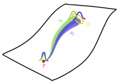
In presence of strong gravitational fields, the phase differences are usually calculated along null-geodesics (see e.g. [14, 16]). In order to evaluate the decoherence of the neutrino WPs in curved spacetime we assume that the ensemble of trajectories for each mass eigenstate is close to null-geodesics. To determine the coherence proper time, a spacetime point $D$ $(t_{D},\vec{x}_{D})$ is considered, at which the WPs can still interefere (Figure 1).

Figure 1: Artistic drawing of a neutrino propagating from a production point P to ”detection” point D where the WPs can still interfere. Each mass eigenstate WP follows a trajectory close to null-geodesics. The coloured widths picture the distribution of trajectories due to the WP finite extension.

3.1 Neutrino trajectories in the Schwarzschild metric

The Schwarzschild metric for a static gravitational field with spherical symmetry is

$$\mathrm{d}s^{2}=-B(r)\mathrm{d}t^{2}+\frac{1}{B(r)}\mathrm{d}r^{2}+r^{2}\mathrm{d}\theta^{2}+r^{2}\sin^{2}{\theta}d\varphi^{2},$$ (32)

where $\left(t,r,\theta,\varphi\right)$ are time, radial distance and angular coordinates and

$$B(r)=1-\frac{r_{s}}{r},~{}~{}~{}~{}~{}~{}r_{s}=2M,$$ (33)

with $r_{s}$ the Schwarzschild radius and $M$ the mass of the central object. Since the gravitational field is spherically symmetric, the neutrino trajectories are confined to a plane. We choose to work in the plane $\theta=\frac{\pi}{2}$. The relevant components of $p_{\mu}^{(j)}$ are

$$p_{t}^{(j)} = -m_{j}B(\vec{r})\frac{\mathrm{d}t}{\mathrm{d}s},$$ (34)

$$p_{r}^{(j)} = \frac{m_{j}}{B(\vec{r})}\frac{\mathrm{d}r}{\mathrm{d}s},$$ (35)

$$p_{\varphi}^{(j)} = m_{j}r^{2}\frac{\mathrm{d}\varphi}{\mathrm{d}s}.$$ (36)

They are related by the mass on-shell relation

$$p_{\mu}^{(j)}p^{(j)\mu}=-m_{j}^{2}.$$ (37)

Since the metric tensor $g_{\mu\nu}$ does not depend on $t$ and $\varphi$, the canonical momentum components

$$E_{j}(\vec{p})\equiv-p_{t}^{(j)},~{}~{}~{}~{}J_{j}(\vec{p})=p_{\varphi}^{(j)},$$ (38)

are constants of motion. They correspond to the energy and the angular momentum of the $j$th mass eigenstate seen by an observer at $r=+\infty$ and therefore differ from those measured by an observer at $D$, or at the production point $P$. Obviously the local energy, measured by an observer at rest at a given spacetime point, can be related to $E_{j}$ through a transformation between the two frames.

The phase argument in (30) can be developed as

$$p_{\mu}^{(j)}\mathrm{d}x^{\mu}=-E_{j}(\vec{p})\mathrm{d}t+\frac{m_{j}}{B(r)}\Big{(}\frac{\mathrm{d}r}{\mathrm{d}s}\Big{)}\mathrm{d}r+J_{j}(\vec{p})\mathrm{d}\varphi.$$ (39)

We consider the case of radial propagation, i.e. $\mathrm{d}\varphi=0$, for which the mass on-shell relation Eq.(37) becomes

$$-B(r)\left(\frac{\mathrm{d}t}{\mathrm{d}s}\right)^{2}+\frac{1}{B(r)}\left(\frac{\mathrm{d}r}{\mathrm{d}s}\right)^{2}=-1.$$ (40)

By using (34) along with $p_{t}^{(j)}=-E_{j}\left(\vec{p}\right)$, Eq.(40) reads

$$\frac{1}{B(r)}\left(\frac{\mathrm{d}r}{\mathrm{d}s}\right)^{2}=-1+\frac{E_{j}^{2}(\vec{p})}{m_{j}^{2}}\frac{1}{B(r)},$$ (41)

which gives

$$\frac{\mathrm{d}r}{\mathrm{d}s}=\sqrt{\frac{E_{j}^{2}(\vec{p})}{m_{j}^{2}}-B(r)},$$ (42)

assuming that neutrinos are propagating outwards. We now introduce general kinematical arguments that will be used to estimate the coherence proper time $\tau_{coh}$.

3.2 A kinematical argument

A clock at the ”detection” point D measures the time delay between the arrival of the WPs of the $j$th and $k$th mass eigenstates propagating along radial geodesics, from P to D. By combining Eqs.(34) and (42) one gets

$$\frac{\mathrm{d}r}{\mathrm{d}t}=B(r)\sqrt{1-\frac{m_{j}^{2}B(r)}{E^{2}_{j}(\vec{p})}}.$$ (43)

By inverting this relation, we get that the $j$th mass eigenstate WP reaches D at the coordinate time

$$t^{j}_{PD}=\int_{r_{P}}^{r_{D}}\frac{dr}{B(r)}{\left[1-\frac{m_{j}^{2}B(r)}{E^{2}_{j}(\vec{p})}\right]}^{-1/2}.$$ (44)

In the limit $m_{j}^{2}B(r)/E^{2}_{j}(\vec{p})\ll 1$, one finds at first order

$$t^{j}_{PD}=\frac{m_{j}^{2}}{2E^{2}_{j}(\vec{p})}r_{PD}+b_{PD},$$ (45)

where the second term is

$$b_{PD}=\int_{r_{P}}^{r_{D}}\frac{dr}{B(r)}=r_{PD}+r_{s}\ln(\frac{r_{D}-r_{s}}{r_{P}-r_{s}}),$$ (46)

with $r_{PD}=r_{D}-r_{P}$. Therefore, from Eqs.(45-46), one gets for the coordinate time delay between the two WPs at D

$$t_{PD}^{jk}=\left[\frac{m_{j}^{2}}{2E^{2}_{j}(\vec{p})}-\frac{m_{k}^{2}}{2E^{2}_{k}(\vec{q})}\right]r_{PD}.$$ (47)

Now, an observer in D will measure a proper time

$$\tau_{D}=t_{D}\sqrt{B(r_{D})},$$ (48)

where we have introduced the WP dispertion in the coordinate time $\sigma_{t}$. Combining (47) and (48) gives the difference between the $j$th and $k$th WPs proper times in D

$$\tau_{D}^{jk}=\sqrt{B(r_{D})}\left[\frac{m_{j}^{2}}{2E^{2}_{j}(\vec{p})}-\frac{m_{k}^{2}}{2E^{2}_{k}(\vec{q})}\right]r_{PD}.$$ (49)

In analogy with the coherence length (14) in flat spacetime, one can define a coherence proper time $\tau_{coh}$ at which the difference in the proper times at D satisfies the following relation

$$\tau={\tau}_{coh}~{}~{}~{}~{}\mathrm{if}~{}~{}~{}~{}\tau^{jk}_{D}=\sigma_{t}\sqrt{B(r_{D})}.$$ (50)

Therefore, from (49)-(50), one gets for the corresponding coordinate distance

$$r^{coh}_{PD}={2E^{2}\over{\Delta m^{2}_{jk}}}\sigma_{x},$$ (51)

with the assumptions that $\sigma_{x}\simeq\sigma_{t}$ and $E_{j}(\vec{p})\simeq E_{k}(\vec{q})\simeq E$. This relation is general and will be used as a comparison for the results based on the density matric approach.

3.3 The density matrix approach

Let us now consider the covariant phase Eq.(30). From Eqs. (39) and (42) one gets for the integral argument, in the case of radial propagation

$$p_{\mu}^{(j)}\mathrm{d}x^{\mu}=-E_{j}(\vec{p})\mathrm{d}t+\frac{1}{B(r)}\sqrt{E_{j}(\vec{p})^{2}-B(r)m_{j}^{2}}\mathrm{d}r.$$ (52)

Neutrinos are assumed to be relativistic at infinity, i.e. $m_{j}(E_{j})^{-1}\ll 1$, which ensures that the conditions is satisfied everywhere on their trajectory. Equation (52) becomes

$$p_{\mu}^{(j)}\mathrm{d}x^{\mu}=-E_{j}(\vec{p})\mathrm{d}t+\frac{1}{B(r)}\left[E_{j}(\vec{p})-\frac{m_{j}^{2}}{2E_{j}(\vec{p})}B(r)\right]\mathrm{d}r.$$ (53)

From Eqs.(30), (46) and (53), the covariant phase reads

$$\phi_{j}(P,D;\vec{p})=-E_{j}(\vec{p})(t_{PD}-b_{PD})-\frac{m_{j}^{2}}{2E_{j}(\vec{p})}r_{PD},$$ (54)

where $t_{PD}=t_{D}-t_{P}$. Consequently, the phase difference $\phi_{kj}=\phi_{k}-\phi_{j}$ is

$$\phi_{kj}(P,D;\vec{p},\vec{q})=(E_{j}(\vec{p})-E_{k}(\vec{q}))(t_{PD}-b_{PD})\\ +\left[\frac{m_{j}^{2}}{2E_{j}(\vec{p})}-\frac{m_{k}^{2}}{2E_{k}(\vec{q})}\right]r_{PD},$$ (55)

and can be written as

$$\phi_{kj}(P,D;\vec{p},\vec{q})=E_{jk}(t_{PD}-b_{PD})+\left(\frac{m_{j}^{2}}{2E_{j}}-\frac{m_{k}^{2}}{2E_{k}}\right)r_{PD}\\ +\vec{v}_{j}(\vec{p}-\vec{p}_{j})\left[t_{PD}-\lambda_{j}r_{PD}\right]-\vec{v}_{k}(\vec{q}-\vec{p}_{k})\left[t_{PD}-\lambda_{k}r_{PD}\right],$$ (56)

by using the first-order expansion (20), with the notation

$$\lambda_{j}=\frac{m_{j}^{2}}{2E_{j}^{2}}r_{PD}+b_{PD}.$$ (57)

Let us now introduce one-body density matrices (18) describing the neutrino mass eigenstates as (non-covariant) Gaussian WPs of width $\sigma_{p}$

$$\rho_{jk}(P,D)=\int_{\vec{p}}\int_{\vec{q}}\exp{\left[-i\phi_{kj}(P,D;\vec{p},\vec{q})\right]}\\ \exp{\left[-\frac{(\vec{p}-\vec{p}_{j})^{2}}{4\sigma_{p}^{2}}-\frac{(\vec{q}-\vec{p}_{k})^{2}}{4\sigma_{p}^{2}}\right]}.$$ (58)

By using (56) the Gaussian integrals can be performed giving the following expression for the elements of the one-body density matrix

$$\rho_{jk}(P,D)=\exp{\{-\sigma_{p}^{2}\left[v_{k}^{2}(t_{PD}-\lambda_{k})^{2}+v_{j}^{2}(t_{PD}-\lambda_{j})^{2}\right]\}}\\ \times N^{\alpha}_{jk}\exp{\left[-iE_{jk}(t_{PD}-b_{PD})+i\left(\frac{m_{j}^{2}}{2E_{j}}-\frac{m_{k}^{2}}{2E_{k}}\right)r_{PD}\right]},$$ (59)

with (19) for the normalisation factor $N^{\alpha}_{jk}$.

We introduce the density matrix integrated over coordinate time

$$\rho_{jk}(r_{P},r_{D})=\int\mathrm{d}t\rho_{jk}(P,D),$$ (60)

and compute the Gaussian integral, which gives

$$\rho_{jk}(r_{P},r_{D})=A_{jk}^{\alpha}~{}\rho^{osc}_{jk}(r_{P},r_{D})~{}\rho^{damp}_{jk}(r_{P},r_{D}),$$ (61)

to be compared with the flat spacetime expression (23). The first exponential term does not depend on $r_{PD}$ and is the same as in flat spacetime (24). It has no influence on neutrino propagation. The second exponential term, that generates neutrino oscillations, is

$$\rho^{osc}_{jk}(r_{P},r_{D})=\exp{\left[i\left(\frac{m_{j}^{2}}{2E_{j}}-\frac{m_{k}^{2}}{2E_{k}}\right)r_{PD}\right]}\\ \times\exp{\left[-i\frac{E_{jk}}{\bar{v}^{2}}\left(v_{k}^{2}\frac{m_{k}^{2}}{2E_{k}^{2}}+v_{j}^{2}\frac{m_{j}^{2}}{2E_{j}^{2}}\right)r_{PD}\right]},$$ (62)

where, in the Schwarzschild metric, $r_{PD}$ does not represent a physical distance. The third and last factor is the damping term responsible for decoherence

$$\rho^{damp}_{jk}(r_{P},r_{D})=\exp{\left[-\frac{({v}_{j}{v}_{k}r_{PD})^{2}}{4\sigma_{x}^{2}\bar{v}^{2}}\left(\frac{m_{k}^{2}}{2E_{k}^{2}}-\frac{m_{j}^{2}}{2E_{j}^{2}}\right)^{2}\right]},$$ (63)

which becomes at first order in $m_{j}/E$

$$\rho^{damp}_{jk}(r_{P},r_{D})\simeq\exp{\left[-\frac{\Delta m_{jk}^{4}r_{PD}^{2}}{32\sigma_{x}^{2}E^{4}}\right]}.$$ (64)

In the flat spacetime limit, $r_{PD}$ becomes the physical distance travelled by neutrinos and this term reduces to the damping term (26) with $r_{PD}$ the coherence length (27). However, if $r_{s}$ is non-null, $r_{PD}$ does not represent a physical distance, while $E$ is not the local energy of the neutrinos but rather the energy at infinity.

In analogy with the flat spacetime case, from Eq.(64) one can define a coherence coordinate distance $r^{coh}_{PD}$ at which the density matrix gets suppressed by $e^{-1}$, namely

$$r^{coh}_{PD}=\frac{4\sqrt{2}\sigma_{x}E^{2}}{\Delta m_{jk}^{2}}.$$ (65)

Note that formally, the expression for $r^{coh}_{PD}$ is the same as the coherence length in flat spacetime (27). The comparison with (51) shows the coherent coordinate distance $r^{coh}_{PD}$ agrees with the expression (51) from kinematical arguments up to $2\sqrt{2}$.

3.4 The coherence proper time

We now use kinematical arguments to relate the derived coherence coordinate distance to a coherence proper time. We start by noticing that the null-geodesics can be used to express the travelled distance as a function of the coordinate time to go from P to D. By using Eqs.(40) and (45), for null-geodesics, one has

$$t_{coh}^{travel}=b_{PD},$$ (66)

and from (48), the coherence proper time is

$$\tau_{coh}=\sqrt{B(r^{coh}_{D})}\left[r^{coh}_{PD}+r_{s}\ln\left(1+\frac{r^{coh}_{PD}}{r_{P}-r_{s}}\right)\right],$$ (67)

where $r^{coh}_{D}=r^{coh}_{PD}+r_{P}$.

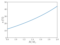
In order to show the impact of strong gravitational fields on the coherence proper time, we present an estimate considering the case of a newly formed neutron star from a core-collapse supernova. Figure 2 shows the relative difference between the coherence proper time (67) and the flat spacetime case (27)

$$\eta=\frac{\tau_{coh}-L_{coh}}{L_{coh}}(\%),$$ (68)

as a function of the Schwarzschild mass $M\in[0.8,2]~{}M_{\odot}$. Neutrinos are emitted at a neutrinosphere of radius $r_{P}=R_{\nu}=10$ km and a typical energy of $E=11$ MeV with $r^{coh}_{PD}$ given by Eq.(65). For the WP width we take $\sigma_{x}\approx 4\times 10^{-12}$ cm [10, 11]. From Figure 2, one can see that the influence of the gravitational field is significant, being of several tens of percent, about $25\%$ ($45\%$) for $1.4M_{\odot}$ ($2M_{\odot}$).

Figure 2: Numerical estimates of the relative difference between the coherence proper time in curved spacetime and the coherence length in flat spacetime, as a function of the Schwarzschild mass $M$.

4 Conclusions

In the present manuscript we have explored neutrino decoherence from WP separation in curved spacetime. To this aim we have extended the WP density matrix formalism used in the context of flat spacetime. We have performed our calculations in the static and spherically symmetric Schwarzschild metric, considering the WPs travel along radial geodesics. We have derived the coherence radial coordinate at a distance from the production point where the WPs still interfere and shown that it is consistent with the one obtained from kinematical arguments. We have then related it to the coherence proper time and provided a numerical estimate showing that the impact of strong gravitation fields on the coherence proper time can be sizable.

This is a first step in the investigation of decoherence effects in presence of strong gravitational fields. Future studies should address the role on the coherence proper time of neutrino interactions with matter and neutrino self-interactions, outside the compact central object. In particular, for adiabatic evolution, a similar procedure could be used based on the matter eigenstate basis. These investigations are necessary to assess if WP decoherence suppresses flavor evolution and its potential impact on the supernova dynamics, $r$-process nucleosynthesis as well as future supernova neutrino observations.

The authors are grateful to Nathalie Deruelle for pointing out the kinematical arguments they have used to define a coherent proper time. They would like to thank Gaetano Lambiase and Carlo Giunti for their comments and acknowledge support from ”Gravitation et physique fondamentale” (GPHYS) and ”Physique Fondamentale et Ondes Gravitationnelles” (PhyFOG) of the Observatoire de Paris.

References

- [1] Y. Fukuda et al. [Super-Kamiokande Collaboration], Phys. Rev. Lett. 81, 1562 (1998) [hep-ex/9807003].
- [2] Q. R. Ahmad et al. [SNO Collaboration], Phys. Rev. Lett. 89, 011301 (2002) [nucl-ex/0204008].
- [3] F. Capozzi, E. Lisi, A. Marrone and A. Palazzo, Prog. Part. Nucl. Phys. 102, 48 (2018) [arXiv:1804.09678 [hep-ph]].
- [4] S. Nussinov, Phys. Lett. 63B, 201 (1976).
- [5] C. Giunti, Found. Phys. Lett. 17, 103 (2004) [hep-ph/0302026].
- [6] C. Giunti and C. W. Kim, Oxford, UK: Univ. Pr. (2007) 710 p
- [7] F. P. An et al. [Daya Bay Collaboration], Eur. Phys. J. C 77, no. 9, 606 (2017) [arXiv:1608.01661].
- [8] G. Barenboim, N. E. Mavromatos, S. Sarkar and A. Waldron-Lauda, Nucl. Phys. B 758, 90 (2006) [hep-ph/0603028].
- [9] G. L. Fogli, E. Lisi, A. Marrone, D. Montanino and A. Palazzo, Phys. Rev. D 76, 033006 (2007) [arXiv:0704.2568].
- [10] J. Kersten and A. Y. Smirnov, Eur. Phys. J. C 76, no. 6, 339 (2016) [arXiv:1512.09068].
- [11] E. Akhmedov, J. Kopp and M. Lindner, JCAP 1709, no. 09, 017 (2017) [arXiv:1702.08338].
- [12] O. L. Caballero, G. C. McLaughlin and R. Surman, Astrophys. J. 745, 170 (2012) [arXiv:1105.6371].
- [13] M. B. Deaton et al., Phys. Rev. D 98, no. 10, 103014 (2018) [arXiv:1806.10255].
- [14] N. Fornengo, C. Giunti, C. W. Kim and J. Song, Phys. Rev. D 56, 1895 (1997) [hep-ph/9611231].
- [15] H. J. Mosquera Cuesta, G. Lambiase and J. P. Pereira, Phys. Rev. D 95, no. 2, 025011 (2017) [arXiv:1701.00431].
- [16] C. Y. Cardall and G. M. Fuller, Phys. Rev. D 55, 7960 (1997) [hep-ph/9610494].
- [17] Y. Yang and J. P. Kneller, Phys. Rev. D 96, no. 2, 023009 (2017) [arXiv:1705.09723].
- [18] H. Duan, G. M. Fuller and Y. Z. Qian, Ann. Rev. Nucl. Part. Sci. 60, 569 (2010) doi:10.1146/annurev.nucl.012809.104524 [arXiv:1001.2799 [hep-ph]].
- [19] M. Tanabashi et al. [Particle Data Group], Phys. Rev. D 98, no. 3, 030001 (2018). doi:10.1103/PhysRevD.98.030001
- [20] C. Volpe, D. Väänänen and C. Espinoza, Phys. Rev. D 87, no. 11, 113010 (2013) [arXiv:1302.2374].
- [21] D. V. Naumov, Phys. Part. Nucl. Lett. 10, 642 (2013) [arXiv:1309.1717].
- [22] L. Stodolsky, Phys. Rev. D 36, 2273 (1987).