MGOS: A Library for Molecular Geometry and Its Operating System

Abstract

The geometry of atomic arrangement underpins the structural understanding of molecules in many fields. However, no general framework of mathematical/computational theory for the geometry of atomic arrangement exists. Here we present “Molecular Geometry (MG)” as a theoretical framework accompanied by “MG Operating System (MGOS)” which consists of callable functions implementing the MG theory. MG allows researchers to model complicated molecular structure problems in terms of elementary yet standard notions of volume, area, etc. and MGOS frees them from the hard and tedious task of developing/implementing geometric algorithms so that they can focus more on their primary research issues. MG facilitates simpler modeling of molecular structure problems; MGOS functions can be conveniently embedded in application programs for the efficient and accurate solution of geometric queries involving atomic arrangements. The use of MGOS in problems involving spherical entities is akin to the use of math libraries in general purpose programming languages in science and engineering.

PROGRAM SUMMARY

Program Title: Molecular Geometry Operating System (MGOS)
Licensing provisions: CC By 3.0
Programming language: C++
Supplementary material: (1) Supplementary Video 1, (2) Supplementary Video 2, (3) Supplementary Video 3, (4) Supplementary Video 4, (5) MGOS manual, and (6) 300 test PDB structure files

Journal reference of previous version: N/A
Does the new version supersede the previous version?: N/A
Reasons for the new version: N/A
Summary of revisions: N/A*

Nature of problem:
For both organic and inorganic molecules, structure determines molecular function and molecular structure is highly correlated with molecular shape or geometry. Hence, many studies were conducted for the analysis and evaluation of the geometry of atomic arrangement. However, most studies were based on Monte Carlo, grid-counting, or approximation methods and a high-quality solution requires heavy computational resources, not to mention about its dependency on computation environment. In this paper, we introduce a unified framework of computational library, Molecular Geometry Operating System (MGOS), based on an analytic method for the molecular geometry of atomic arrangements. We believe that the powerful MGOS application programming interface (API) functions will free scientists from developing and implementing complicated geometric algorithms and let them focus on more important scientific problems.

Solution method:
Molecular Geometry (MG) is a general framework of mathematical/computational methods for solving molecular structure problems using a geometry-priority philosophy and is implemented by MGOS which is a library of callable C++ API functions. MGOS is developed based on the Voronoi diagram of three-dimensional spheres and its two derivative constructs called the quasi-triangulation and beta-complex. Note that this Voronoi diagram is different from the ordinary Voronoi diagram of points where the points are atom centers. Being an analytic method, the solutions of many geometric queries on atomic arrangement, if not all, are obtained correctly and quickly. The MGOS architecture is carefully designed in a three-tier architecture so that future modifications and/or improvements can be reflected in the application programs with no additional programming by users.

Additional comments including Restrictions and Unusual features: N/A

1 Introduction

In physics, chemistry, and materials science, the properties of inorganic molecules result from the arrangement of their atoms [1, 2, 3]. In biology, the structure of biomolecules determines their function [4, 5, 6, 7, 8, 9]. A molecule’s properties and interactions with its environment depend on the geometrical arrangement of its atoms, and geometry has long been one of key issues in the study of atomic arrangements. In physics and materials science, examples include the diffusion of lithium ions through paths closely correlated with geometric channels [1]; the porosity and surface area of metal organic framework (MOF) for hydrogen storage [2, 3], water content regulation in polymer membranes through nanocracks which work as nanoscale valves [10], to name a few. In biology, classic examples are the shape complementarity of the double-helix structure of DNA [11, 12], and the lock-and-key [13] and induced-fit theories [14] of small-molecule binding to proteins. There are many other examples: the linear relationship between hydrophobic energy and the loss of solvent accessible surface area [4]; the effect of voids on the solvation and hydration of proteins [6]; the channel structure of ion channels and pumps across cell membranes [7] and in the ribosome for protein synthesis [8]; ferritin as a protein nanocage for iron storage [9]; the Connolly surface of proteins [5]. The examples assert that accurate and efficient geometric computation is critical for understanding and designing molecules.

However, many studies to date on molecular geometry problems have mostly been based on Monte Carlo simulation, counting grid points, or approximations. For instance, molecular volume is commonly estimated by counting the numbers of random points or grid points contained in the molecule [15]; conversely, molecular voids are recognized by removing these grid points [16]. Another example is the imprecise estimation of solvent accessible surfaces [17], which is critical for solvation models used in the calculation of electrostatic energy.

Fig. 1 shows the comparison between an analytic [18, 19] and a grid-counting [16] method for computing molecular voids using a test data set consisting of 300 biomolecular structures from the Protein Data Bank (PDB [20]). See Appendix I for the 300 PDB codes. In Fig. 1(a), the horizontal axis denotes the size (i.e. the number of atoms) of each molecule of the test set and the vertical axis denotes the number of computed voids in the molecular boundary in which at least one water molecule can be placed. Water molecules are modeled as spherical probes of radius 1.4Å. The red filled circle corresponds to the output from the BetaVoid program [18] which implements an analytic method using the Voronoi diagram of three-dimensional spherical atoms. The other three types of mark denote the results computed by the VOIDOO program (http://xray.bmc.uu.se/usf/voidoo.html) [16] corresponding to the grid resolutions of 0.1, 0.5, and 1.0. Fig. 1(b) is a zoom-in of the red rectangular box of Fig. 1(a). Note that VOIDOO finds fewer voids than BetaVoid does. Fig. 1(c) and (d) show the total volume of all the computed voids and Fig. 1(e) and (f) show the computation time taken by the programs. The following observations were made. Compared to the correct solutions computed by the BetaVoid program, VOIDOO finds fewer voids (i.e., it misses many small voids) but significantly overestimates void volumes (despite missing many voids) while it takes significantly more computation time than BetaVoid. VOIDOO, at 0.1Å grid-resolution, crashes on many moderately sized molecules due to memory shortage. This experiment clearly shows how an analytic approach compares with an inaccurate and inefficient approach using grid points. The experiment was performed on a personal computer with Inter Core i5-4670 CPU (3.4GHz), 8 GB RAM, and Windows 7 Enterprise K (64 bit).

The use of such resolution-dependent approaches is common despite their unreliable, inconsistent, and sometimes conflicting results [21]. We observe that VOIDOO is still popular in diverse disciplines [22, 23, 24, 25, 26, 27, 28, 29, 30, 31, 32] and studies of grid-based algorithms continues [33]. The absence of an overarching analytical theory is because individual researchers have focused on problem-specific, local aspects of geometry problems, concentrating on isolated issues such as surfaces, voids, channels, volumes, areas, and so on. With so many independently developed methods, it has been hard to build a general computational framework for accurately and efficiently solving all these types of geometrical problems.

Here we introduce “Molecular Geometry (MG)” as a general framework of mathematical/computational methods for solving molecular structure problems in geometry-priority approaches, and describe the “MG Operating System (MGOS)” which is a library of callable C++ routines for implementing the MG approach in analytical methods. The proposed analytical methods are based on the Voronoi diagram of three-dimensional spheres [34], the quasi-triangulation [35, 36], and the beta-complex [37]. The MG/MGOS method has three primary advantages: application independence, researcher productivity, and solution correctness/accuracy. In other words, equipped with MG/MGOS, researchers from diverse disciplines can conveniently and easily build computational models to solve molecular geometry problems and quickly obtain correct (or accurate) solutions.

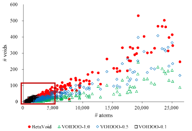
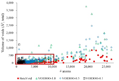
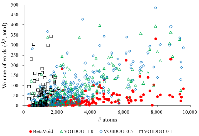
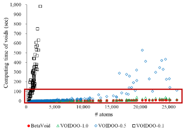
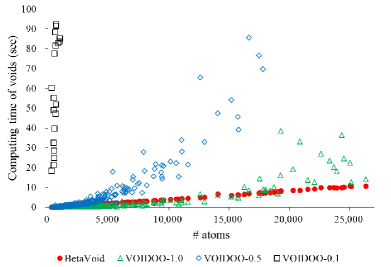
Figure 1: Lee-Richards voids corresponding to a water molecule probe (i.e. 1.4Å radius) computed by BetaVoid [18] and VOIDOO [16]. The test set consists of 300 PDB structures (Appendix 1 lists the PDB codes). The red circles correspond to BetaVoid results; VOIDOO-1.0, VOIDOO-0.5, and VOIDOO-0.1 corresponds to grid resolutions of 1.0, 0.5, and 0.1 Å in VOIDOO, respectively. The right column is a zoom-in of the left column. (a) and (b) The number of recognized voids; (c) and (d) The total volume of the recognized voids; (e) and (f) Computation time.

Section 2 briefly reviews the evolution of the geometry concepts applied to atomic arrangements for materials and biomolecules. Section 3 introduces Molecular Geometry as a new computational discipline for studying atomic arrangements. Section 4 introduces the Molecular Geometry Operating System as a tool for implementing MG. Section 5 presents two example molecular geometry problems solved by MGOS. Section 6 presents the application-neutral architecture of MGOS. Section 7 concludes.

2 How the geometry concept has evolved in the molecular world

Johannes Kepler’s treatise The Six-cornered Snowflake in 1611 and Robert Hooke’s book Micrographia in 1665 might be the earliest observations of crystallization as a sphere packing process. In Cristallographie in 1783, Rome de L’Isle treated geometry and chemical composition with an equal importance to characterize mineral properties and found “the law of the constancy of interfacial angles” which became the foundation of crystallography. Before the advent of X-ray crystallography, crystals were primarily studied from a geometry perspective. In 1805, John Dalton introduced the concept of the spherical atom as the indivisible unit of matter and in 1874, Le Bel and Van’t Hoff independently introduced the concept of tetrahedrally coordinated carbon atoms [38, 39]. This became the foundation of modern stereochemistry which is the basis of the study of molecular structures [40]. Understanding steric effects (i.e. each atom occupies a certain amount of space) is the basis of the stereochemistry of atoms and provides a geometric understanding of the molecular world. The coordination number of an atom, defined by Werner in 1893, is still a commonly used geometric measure of atomic arrangement.

In 1940, Sidgwick and Powell proposed that molecular structure is determined by the electron pairs in the valence shell [41, 42]. This idea was developed in 1957 by Gillespie and Nyholm  [43] into what is now known as the valence shell electron pair repulsion (VSEPR) model, the name proposed in 1963 [44], which has been used for predicting molecular structure using the Pauli Exclusion Principle, but without solving any explicit equation. VSEPR is one of the simplest and most successful models of molecular structure  [45, 44], and remains popular. VSEPR can be viewed as a geometric approach to understanding the molecular world.

Molecular biology is the molecular world where geometry has arguably received the most attention. In 1890, Emil Fischer proposed the well-known lock-and-key theory to explain the interactions between biomolecules. This is an excellent example of modeling biomolecular phenomena through geometry [13, 46]. In 1953, the year that the double-helix structure of DNA was discovered, Francis Crick suggested the idea of a computational approach to the binding between two small molecules through their surfaces [47]. Crick posited that shape complementarity in the helical coiled coil could be modeled as knobs fitting into holes. This could be the first proposal of explicitly using geometry to understand molecular phenomena, and became the basis of molecular docking. In 1958, Koshland extended the lock-and-key theory to propose the induced-fit theory [14, 48, 49].

The first determination of the three-dimensional structure of a protein was performed by John Kendrew and Perutz in 1960 [50] when they solved the structure of myoglobin. Since then, protein structure determination has become almost routine work; and the PDB contains 152,500 biomolecular structures as of June 8, 2019 [20]. Given atomic arrangement databases, such as the PDB, geometry analysis becomes one of the most important research topics for researchers. Cavities in biomolecules are fundamental for function, stability, dynamics, ligand binding, etc. The first computational study of cavities in proteins was reported by Lee and Richards in 1971 [51]. Chothia in 1974 found that the hydrophobic energies in proteins are directly related to the solvent accessible surface area of both polar and non-polar groups, and reported the linear relationship between the hydrophobic energy of proteins and the loss of solvent accessible surface area during folding [4, 52]. This demonstrates that the atoms in folded globular proteins tend to be tightly packed. Thus a large residue volume, and consequently a low overall density, suggests the model of the protein is a poor one and, conversely, a small volume, and high density, suggests is it more likely to be a good one [52]. A protein’s interior is closely packed, with few cavities, so that no water molecules are trapped in non-polar cavities [52, 53]. The dense packing is critical in stable folding, and residue volumes are directly related to packing energies and conformational entropies. The stable aggregation of secondary structures increases their interaction area to achieve a high hydrophobicity and results in an increased molecular density.

In the case of enzymes, which are globular proteins, the optimal way of minimizing the volume and the solvent accessible surface area while keeping a constant potential energy is to make the shape as spherical as possible with as few cavities as possible. Due to the potential energy constraint, the overlap between atoms is limited at a certain level. Therefore, this is a geometric optimization problem of packing spherical atoms in a spherical container of an appropriate size. However, certain geometric features need to be conserved for the molecule to maintain its function. For example, proteasomes require their channel structures for disassembling proteins, ribosomes need to conserve their channels for synthesizing proteins, while membrane proteins require channels for the passage of ions. Therefore, to minimize both volume and accessible surface area under the potential energy constraint, while preserving their crucial geometric features, the interior voids of these proteins must be somehow minimized. Hence, the accurate computation of voids in a molecular structure is important for the assessing the structure. In this regard, the recognition of molecular cavities, such as channels and voids, the computation of their global properties, and understanding their topological structures are fundamental. As the data in the PDB has been more frequently used, the importance of taking into account its quality has also increased, and there are now a number of tools for assessing structural quality [54, 55, 56].

3 Molecular Geometry: A New Approach to Study Atomic Arrangement

Fig. 2 shows the computational process of solving molecular problems. In Fig. 2(A), Mapping I depicts the traditional approach of going directly from a particular molecular problem $\mathcal{M}$ to its solution $Sol(\mathcal{M})$. There are uncountably many molecular problems and each problem can have alternative mappings because its modeling is dependent on the nature of the study. This leads to uncountably many instances of Mapping I. Each mapping instance usually consists of nontrivial computational steps and almost always contains a geometry subproblem involving spherical objects, which in many cases are van der Waals atoms. Earlier studies [1, 2, 3, 4, 5, 6, 7, 8, 9] show this issue is real and highly common. Surprisingly, many seemingly easy geometry problems among spheres remain challenging, if not computationally hard to solve, because of a lack of a suitable mathematical/computational framework. Therefore, researchers often spend a significant amount of time and effort, in the course of solving their geometry problems, developing and implementing their own algorithms. Furthermore, due to the complexity of the geometry problems, researchers usually employ Monte Carlo simulation, grid counting, or other approximate methods.

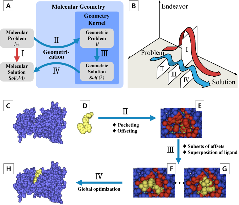
Figure 2: The Molecular Geometry (MG) framework. (A) The MG approach (Mappings II, III and IV) vs. the traditional approach (Mapping I). (B) The human effort (for developing and implementing algorithms) and computational cost of the MG and traditional approaches. (C) Receptor. (D) Ligand. (E) Pocket. (F) and (G) Two initial docking poses. (H) Optimal docking solution.

MG provides an alternative, orthogonal method to this traditional approach. It bypasses the time-consuming and error-prone Mapping I by taking the walk-around path consisting of Mappings II, III, and IV. First, the problem $\mathcal{M}$ is modeled as a geometry problem $\mathcal{G}$ involving spherical atoms (Mapping II). Then, $\mathcal{G}$ is solved via geometric theorems to give the solution $Sol(\mathcal{G})$ (Mapping III) which is back-transformed to $\widehat{Sol}(\mathcal{M})$ in the original molecular space (Mapping IV). The thesis is that $\widehat{Sol}(\mathcal{M})\approx Sol(\mathcal{M})$, possibly with some preconditions. The forward and backward transformations of Mappings II and IV are together called the geometrization while the computational methods for Mapping III form the geometry kernel. The geometrization and geometry kernel together form the basis of the discipline MG (which is different from the earlier notion [42]).

$\widehat{Sol}(\mathcal{M})$ is either close enough to, or a good approximation of, $Sol(\mathcal{M})$ to allow a more intensive computational process such as a molecular dynamics (MD) simulation to be launched. As the computational cost of the walk-around path of Mappings II, III, and IV is significantly cheaper than that of Mapping I, the path may iterate as many times as necessary by refining the geometrization. If the criteria for the convergence of $\widehat{Sol}(\mathcal{M})$ can be defined, the solution process can iterate, possibly without human intervention. Physicochemical and biological properties should be carefully reflected during the geometrization. Given a proper geometrization and a geometry kernel, the path might be automated to iterate if necessary. Fig. 2(B) depicts the significant reduction of both human effort and computational requirement by the MG approach.

Fig. 2(C) through (H) illustrate how a docking simulation program can adopt MG/MGOS in its algorithm. Given a receptor (C) and a ligand (D) for docking, it is desirable to identify a pocket (E) on the receptor surface where the ligand might bind (Mapping II). Then, the conformation of the ligand within the pocket can be found by minimizing the distance between the atom sets of both the ligand and the pocket, where the distance is defined by a geometric measure that can be easily evaluated (F and G) (Mapping III) [57]. Multiple conformations can be found quickly. The ligand conformations can then be used as initial solutions for a global optimization procedure such as the genetic algorithm using a fitness function reflecting the physicochemical and biological measures (H) (Mapping IV). It turns out that the geometrical best-fit solutions using van der Waals radii for atoms are often sufficiently close to the global solution. [58] is another example for side-chain prediction.

The MG approach has two preconditions: a mathematically and computationally well-established geometry kernel and a physicochemically and biologically well-defined geometrization. The MGOS engine’s geometry kernel is written in standard C++ and is based on the Voronoi diagram of three-dimensional spheres [34] and its two derivative constructs [37]. The geometrization is inevitably domain-dependent and is somewhat empirical. For example, different sets of atomic radii may be used for different problems [59, 60]. The effective Born radius [61, 62] may be most appropriate when using the generalized Born approximation of the Poisson-Boltzmann equation to account for the electrostatic contribution to solvation energy. In studying a potassium channel’s recognition selectivity, its dependence is likely to be on ion radius rather than charge density [63]. The analysis of protein packing, protein recognition and ligand design [64], etc will be governed by the radii of different atomic groups. Previous studies [1, 2, 3, 4, 5, 6, 7, 8, 9] can be interpreted as efforts at applying different types of geometrization. A set of geometrization primitives and parameters for each and every application domain should be defined through theoretical studies, experiments, and collaborative thoughts.

4 MGOS: The Engine to Implement MG

MGOS implements MG. The usefulness of MGOS is akin to a math library for general-purpose programming languages in science and engineering. Imagine the time and effort it would take a researcher, even with good programming skills, to code from scratch an algorithm for evaluating, say, $\sin(1.23)$ or $\sqrt{2}$, without a math library. Would the code be accurate and efficient enough? Any complicated scientific problem is likely to require calls to many such functions, so could one effectively develop an effective program without such a math library?

MGOS consists of a set of natural-language-like application programming interface (API) functions, easily callable from application programs (see Appendix II for the list of current MGOS APIs) and efficiently provides a correct/accurate solution of geometric queries involving the arrangements of spherical objects where the objects are frequently van der Waals atoms. For example, the compute_volume_and_area_of_van_der_Waals_model() command computes the volume of the space taken by the atoms (with the van der Waals radii) of a given molecule. The name of the command is clear about its function. The compute_voids_of_Lee_Richards_model() command finds all interior voids where an a priori defined spherical probe can be placed (e.g. a sphere with 1.4Å radius for water) and computes void properties. Computed voids can be further processed. For instance, the voids can be sorted according to volume or boundary area; the atoms whose boundary contribute to each void can be reported; the segment of the atom boundary contributing to the void can be identified and its area computed, etc.

An early attempt at a formal theory to investigate the geometry of atomic arrangement was based on the ordinary Voronoi diagram of points, originally used by Bernal and Finney in 1967 for analyzing liquid structure composed of monosized atoms [65]. Being the most compact representation of proximity among points, the ordinary Voronoi diagram, and its dual called the Delaunay triangulation, has proved the best method for solving spatial problems for points [66]. To extend the theory from points to polysized spheres, we use the Voronoi diagram of spheres [34], also called the additively-weighted Voronoi diagram, which correctly recognizes the Euclidean proximity among the spherical objects between any pair of nearby spheres. Our Voronoi diagram of spheres, along with its derivative structures, the quasi-triangulation [35, 36] and the beta-complex [37], provides a powerful computational platform for mathematically rigorous, algorithmically correct, computationally efficient, and physicochemically and biologically significant, and practically convenient method for any geometry problem involving spherical atoms.

5 Use Cases

We show here how a few simple MGOS APIs can be used to easily compute otherwise difficult to compute geometric features such as voids, channels, water-exposed atoms, etc. of a protein consisting of many atoms.

5.1 Case I: Analysis of an atomic arrangement

Fig. 3 shows a protein structure (PDB id: ijd0) with more than 4,000 atoms. We want to find the boundary atoms exposed to water molecules (modeled as spheres of 1.4Å radius), and buried atoms. Then, we want to find voids which can contain water molecules and any channel structures that allows the passage of water molecule.

Fig. 3(A) shows the space-filling, or CPK-model, of the protein structure. Observe that there is a tiny hole corresponding to a channel penetrating the structure. Fig. 3.(B) shows the quasi-triangulation computed by the MGOS API commands in block B1. The command MG.preprocess() computes the Voronoi diagram of the input atoms and transforms it to the quasi-triangulation. Fig. 3(C) shows the beta-complex corresponding to water molecules (i.e. spherical probes with 1.4Å radius). Fig. 3(D) and (D’) show the atoms exposed to and buried from bulk water, respectively (computed by block B2). Hence, the union of the structures in Fig. 3(D) and (D’) is the input structure in Fig. 3(A). Note that the challenging task of the correct and efficient computation of these structures can be easily and conveniently done by calling a few MGOS APIs. Fig. 3(E) shows the voids (green) that may host one or more water molecule (from a geometric point of view) where the molecule is displayed by a ball-and-stick model. The voids were computed by the program segment in B3. Fig. 3(F) shows the largest (by volume) of the recognized voids, and the atoms whose boundaries contribute to the boundary of this void. We call these atoms the contributing atoms. If it is necessary to investigate if a water molecule can indeed be placed in the void, the biochemical or biophysical properties of the surface segments of the void boundary can be further analyzed by computing the precise geometric information of the patches of atomic boundaries using MGOS APIs. In fact, the compute_voids_of_Lee_Richards_model( WATER_SIZE ) finds all voids that may contain water molecule(s), computes the volume of each void, computes the boundary area of each void, finds the contributing atoms, computes the area of the contributing patch(es) of each contributing atom, etc. The program segment in B4 simply returns the contributing atom information already computed by the command above. Fig. 3(G) shows the channels that may allows a water molecule to move. Like the voids, the surface properties of these channels can be further investigated if necessary. These channels were computed by the program segment in B5. Fig. 3(H) and (I) show two different visualizations of the biggest channel with its contributing atoms and spine, respectively. This biggest channel is located by the program segment in B6. Refer to Supplementary Video 1 for the three-dimensional animation of this computational process.

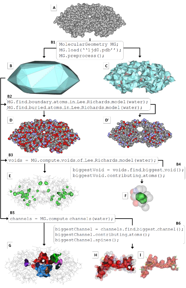
Figure 3: Protein structure analysis using Program-Use-Case-I in Fig. 4 (PDB code: 1jd0; 4,195 atoms). See Supplementary Video 1. (A) and (B) The space-fillin and quasi-triangulation models of the input structure. (C) The beta-complex for water (i.e. a spherical probe with radius 1.4Å). (D) and (D’) The atoms exposed to and buried from bulk water, respectively. (E) The (green) voids for water. (F) The largest void and its contributing atoms. (G) The channels for water. (H) and (I) Two different visualizations of the biggest channel with its contributing atoms and spine, respectively.

/* Program-Use-Case-I: Analysis of single atomic arrangement */ // include a head file for using MGOS 1 #include "MolecularGeometry.h" 2 using namespace MGOS; // define the probe size for water molecule 3 const double WATER_SIZE = 1.4; 4 int main() 5 { // B1: load a PDB model and preprocess 6 MolecularGeometry MG; 7 MG.load( "1jd0.pdb" ); 8 MG.preprocess(); // B2: find the atoms on boundary and of interior corresponding to water molecule 9 AtomPtrSet boundaryAtoms = MG.find_boundary_atoms_in_Lee_Richards_model( WATER_SIZE ); 10 AtomPtrSet interiorAtoms = MG.find_buried_atoms_in_Lee_Richards_model( WATER_SIZE ); // B3: compute the voids inside the protein which are defined by water molecule size 11 MolecularVoidSet voids = MG.compute_voids_of_Lee_Richards_model( WATER_SIZE ); // B4: find the biggest void and its contributing atoms 12 MolecularVoid biggestVoid = voids.find_biggest_void(); 13 AtomPtrSet contributingAtomsOfBiggestVoid = biggestVoid.contributing_atoms(); // B5: compute the channels inside the protein which are defined by water molecule size 14 MolecularChannelSet channels = MG.compute_channels( WATER_SIZE ); // B6: find the biggest channel, its contributing atoms, and spines 15 MolecularChannel biggestChannel = channels.find_biggest_channel(); 16 AtomPtrSet contributingAtomsOfBiggestChannel = biggestChannel.contributing_atoms(); 17 biggestChannel.spine(); 18 return 0; 19 }

Figure 4: Program-Use-Case-I computes the voids, channels, etc. in Fig. 3

Program-Use-Case-I in Fig. 4 is the complete code of an application program which embeds the MGOS APIs to perform the required computation. The first line of the code includes the MolecularGeometry.h file which defines the MGOS classes to be used by the program. Line 7 loads an input file of PDB format. The MG.preprocess() command in line 8 computes the Voronoi diagram of the input structure and transforms it to its quasi-triangulation. If the quasi-triangulation file already exists in the working directory, this command directly loads the file.

The command MG.find_boundary_atoms_in_Lee_Richards_model() in line 9 finds the set of boundary atoms of the Lee-Richards solvent accessible model where the solvent is represented as a spherical probe for water with the radius 1.4Å, as defined in line 3. Similarly, MG.find_buried_atoms_in_Lee_Richards_model() finds the set of buried atoms of the Lee-Richards solvent accessible model. It is worth noting that without the MGOS engine, it is very difficult to correctly and efficiently find these sets because it is necessary to distinguish the atoms exposed to solvent from those that are buried.

The command MG.compute_voids_of_Lee_Richards_model() in line 11 locates all voids inside the Lee-Richards solvent accessible model. After finding the voids, this command computes the geometric properties such as the volume and area of each void. Then, voids.find_biggest_void() in line 12 finds the void with the biggest volume. The command biggestVoid.contributing_atoms() in the next line finds all the atoms contributing to the boundary of the biggest void.

MG.compute_channels() in line 14 computes all of the channels inside the Lee-Richards solvent accessible model. channels.find_biggest_channel() in line 15 finds the biggest channel and the atoms contributing to the boundary of this biggest channel are given by
biggestChannel.contributing_atoms(). biggestChannel.spine() in line 17 finds the spine of the biggest channel.

Fig. 5, together with Supplementary Videos 2, 3, and 4, show other examples of voids and channels that can be recognized by a slight modification of the Program-Use-Case-I code with ferritin, a potassium channel, and a metal-organic framework.

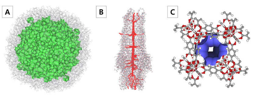
Figure 5: Geometric features in atomic arrangements shown in ball-and-stick diagram. See Supplementary Video 2, 3, and 4. (A) Ferritin (PDB code: 1mfr; 34,320 atoms). The largest void (green) for water (modeled as a sphere of 1.4Å radius). 492 tiny voids are additionally found but are not shown here because they are biologically insignificant. (B) Potassium channel protein (PDB code: 2vdd; 9,915 atoms) showing a potassium channel (red). (C) Metal organic framework MOF5 [2] and its Lee-Richards accessible surface (blue) corresponding to a 2.0Å spherical probe. The geometric properties such as the pore volume, apparent surface area, etc. are critical for MOF design.

5.2 Case II: Analysis of 100 atomic arrangements

Fig. 6 shows the code of another application program, Program-Use-Case-II, which analyzes multiple PDB files to compute the volumes, areas, and voids of 100 molecular structures (arbitrarily selected for demonstration purpose) together with the computation time statistics.

/* Program-Use-Case-II: Analysis of multiple atomic arrangements */ // include a head file for using MGOS 1 #include "MolecularGeometry.h" 2 using namespace MGOS; // include a head file for using file I/O functions 3 #include "MGUtilityFunctions.h" // define the extension of PDB file. 4 const string PDBFileExtension(".pdb"); 5 int main(int argc, char* argv[]) 6 { // open a file which contains the list of PDB codes 7 ifstream fileFor100PDBCodes( argv[ 1 ] ); // get the number of PDB files 8 int numberOfPDBFiles = get_the_number_of_PDB_files( fileFor100PDBCodes ); // get the solvent probe radius 9 double solventProbeRadius = atof( argv[ 2 ] ); // open a blank file for writing the result 10 ofstream fileForMassPropertyAndVoidStatistics( argv[ 3 ] ); // write the column names in the first line of the file 11 write_column_names_of_output_file( fileForMassPropertyAndVoidStatistics ); // process each and every PDB model 12 int i_PDB; 13 for (i_PDB = 0;i_PDB < numberOfPDBFiles;i_PDB++) 14 { // get current PDB code 15 string currentPDBCode = get_current_PDB_code( fileFor100PDBCodes ); // load a PDB model, preprocess, and measure elapsed time 16 MolecularGeometry MG; 17 MG.load( currentPDBCode + PDBFileExtension ); 18 MG.preprocess(); 19 double timeForVDQT = MG.elapsed_time(); // compute volume and area, and measure elapsed time 20 MolecularMassProperty massProperty 21 = MG.compute_volume_and_area_of_Lee_Richards_model( solventProbeRadius ); 22 double timeForVolumeAndArea = MG.elapsed_time(); // compute void, and measure elapsed time 23 MolecularVoidSet voids 24 = MG.compute_voids_of_Lee_Richards_model( solventProbeRadius ); 25 double timeForVoid = MG.elapsed_time(); // write the statistics of current model 26 write_statistics_for_current_PDB_model(currentPDBCode, MG, massProperty, voids, timeForVDQT, 27 timeForVolumeAndArea, timeForVoid, fileForMassPropertyAndVoidStatistics); 28 } 29 return 0; 30 }

Figure 6: Program-Use-Case-II that computes the volumes, areas, and voids of 100 molecular structures

Program-Use-Case-II requires four pieces of input data: (i) A file containing PDB codes (Fig. 7), (ii) the size of the solvent probe, (iii) the output file to store computed results (Fig. 7), and (iv) the PDB model files.

100 1c26
1d2k
$\vdots$ 4eug

code, #atoms, volume, area , #voids, T(VD/QT), T(mass), T(void) 1c26, 268, 7410.01, 2393.33, 0, 514 , 110, 78 1d2k, 3082, 66165.1, 4179.02, 47, 7990 , 952, 936 4eug, 1788, 39124.8, 3710.06, 11, 3748 , 484, 406

Figure 7: Examples of files for Program-Use-Case-II: (a) The input file storing the 100 PDB codes. (b) The output file for computation result.

The program begins by including MGUtilityFunctions.h in addition to MolecularGeometry.h because the program also uses some utility functions related to file I/O. The command in line 7 opens a file, say FILE_IN, which contains the 100 PDB codes to use. The first line of FILE_IN contains the number 100 of PDB models. Each of the following lines contains a PDB code as shown in Fig. 7(a). The next command get_the_number_of_PDB_files() returns “100” by referring to the first line of FILE_IN. Line 9 sets the size of the solvent probe from the command line invoking program execution. Line 10 opens a blank output file, say FILE_OUT, for the computed results. The command write_column_names_of_output_file() writes the column names to the first line of FILE_OUT as shown in Fig. 7(b).

The code chunk in lines 12–28 processes each PDB model by computing geometric features, measuring the elapsed times, and writing the results to FILE_OUT. Line 15 gets the current PDB code from FILE_IN and the corresponding PDB model is loaded by line 17. After the model is preprocessed in line 18, the elapsed time is given by the command MG.elapsed_time() in the next line. MG.compute_volume_and_area_of_Lee_Richards_model() in line 21 computes the volume and area for the Lee-Richards solvent accessible model. The program also counts the elapsed time in the next line. Similarly, MG.compute_voids_of_Lee_Richards_model() in line 24 computes the voids for the solvent molecule and then, the elapsed time is counted. The command write_statistics_for_current_PDB_model() in lines 26 and 27 writes the statistics for the current PDB model, such as PDB code, the number of atoms, volume, area, the number of voids, and time statistics as in Fig. 7(b). The code for MGUtilityFunctions used in Program-Use-Case-II is shown in Fig. 8.

/* MGUtilityFunctions */ 1 #include "MGUtilityFunctions.h" 2 int get_the_number_of_PDB_files(ifstream& fileFor100PDBCodes) 3 { // get the number of PDB files by interpreting the first line as an integer 4 const int bufferSize = 100; 5 char line[bufferSize]; 6 fileFor100PDBCodes.getline(line, bufferSize); 7 char* delims = "\n \t"; 8 char* token = strtok(line, delims); 9 int numberOfPDBFiles = std::atoi( token ); 10 return numberOfPDBFiles; 11 } 12 void write_column_names_of_output_file(ofstream& fileForMassPropertyAndVoidStatistics) 13 { 14 fileForMassPropertyAndVoidStatistics $\ll$ "PDBFileName," 15 $\ll$ "numberOfAtoms," $\ll$ "volume," $\ll$ "area," $\ll$ "numberOfVoids," 16 $\ll$ "time(VD/QT)," $\ll$ "time(mass)," $\ll$ "time(void)" $\ll$ endl; 17 } 18 string get_current_PDB_code(ifstream& fileFor100PDBCodes) 19 { // get the current PDB code by interpreting the current line as a string 20 const int bufferSize = 100; 21 char line[bufferSize]; 22 fileFor100PDBCodes.getline(line, bufferSize); 23 char* delims = "\n \t"; 24 char* token = strtok(line, delims); 25 string currentPDBCode = string( token ); 26 return currentPDBCode; 27 } 28 void write_statistics_for_current_PDB_model( 29 const string& currentPDBCode, MolecularGeometry& MG, 30 MolecularMassProperty& massProperty, MolecularVoidSet& voids, 31 const double& timeForVDQT, const double timeForVolumeAndArea, 32 const double timeForVoid, ofstream& fileForMassPropertyAndVoidStatistics) 33 { // get the statistics such as the number of atoms, volume, area, and the number of voids 34 int numberOfAtoms = MG.number_of_atoms(); 35 double volume = massProperty.volume(); 36 double area = massProperty.area(); 37 int numberOfVoids = voids.number_of_voids(); // write the statistics in the output file 38 fileForMassPropertyAndVoidStatistics $\ll$ currentPDBCode $\ll$ "," 39 $\ll$ numberOfAtoms $\ll$ "," $\ll$ volume $\ll$ "," $\ll$ area $\ll$ "," $\ll$ numberOfVoids $\ll$ "," 40 $\ll$ timeForVDQT $\ll$ "," $\ll$ timeForVolumeAndArea $\ll$ "," $\ll$ timeForVoid $\ll$ endl; 41 }

Figure 8: MGUtilityFunctions which are used in Program-Use-Case-II.

Fig. 9 shows the graphs produced by using Microsoft Excel with the output file FILE_OUT for some computed results for the 100 PDB files. Fig. 9(a), (b), and (c) are the volumes, areas, and the numbers of voids, respectively. Fig. 9(d) shows the time for computing the Voronoi diagram and quasi-triangulation. Fig. 9(e) is the time for computing the volume and area, and Fig. 9(f) for the voids. Note that these graphs can be produced by a few clicks of the mouse button and column choices.

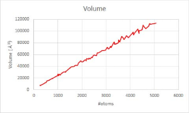
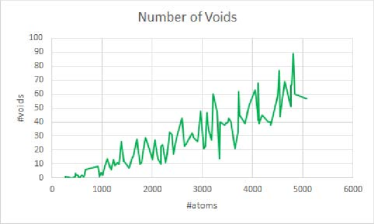
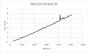
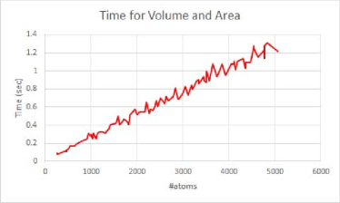
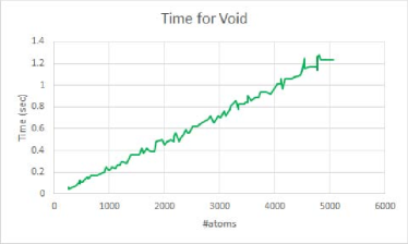
Figure 9: Graphs produced by Microsoft Excel using the output file FILE_OUT. Volume, area, the number of voids, and time statistics for the 100 PDB models, ordered by the total number of atoms: (a) volumes, (b) areas, (c) the numbers of voids, (d) time for computing Voronoi diagram and its quasi-triangulation, (e) time for volumes and areas, and (f) time for voids.

6 MGOS Architecture

The architecture of MGOS has been carefully designed so that any future modifications will not require rewriting the existing code of an application program. If a molecular problem can be properly geometrized in terms of appropriate-sized spherical balls, the MG/MGOS framework can quickly provide the best possible solution. It is expected that the MGOS engine will evolve, with new functions to be added in the future. One area of interest is in developing methods for the optimal design of molecules in the concept of “operating system”, e.g. in terms of side chain conformations, to develop a program to help engineer proteins.

Software architecture: MGOS is middleware, connecting application programs with a low-level Geometry Library performing geometric computations (Fig. 10). It is composed of a set of API functions callable from application programs; each is implemented by calls to the Geometric Library’s functions which are application-independent. In addition to geometric properties, MGOS also makes use of molecular properties such as force-fields, electostatics, etc.

The Geometric Library, the application-independent low level library, performs geometric computations among spherical objects and is based on three closely related constructs: the Voronoi diagram of three-dimensional spheres, the quasi-triangulation, and the beta-complex.

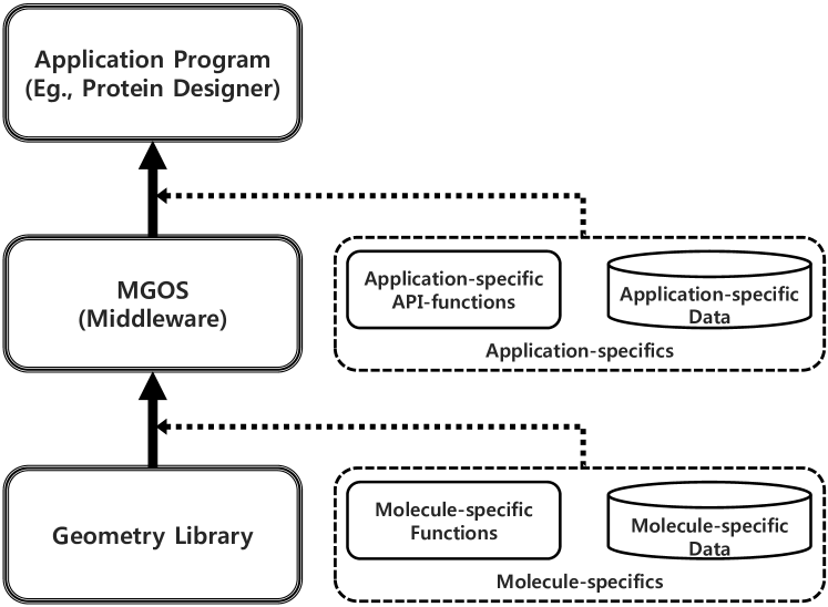
Figure 10: The role of MGOS for creating application programs. MGOS is a middleware engine connecting application programs to a set of appropriate API-functions where each performs the required geometric computation.

Topology data structure: Fig. 11 shows the design of the fundamental data structure for topology in the MGOS library. Three types of Voronoi diagrams (i.e., the ordinary Voronoi diagram of points, the power diagram, and the Voronoi diagram of spherical balls) are all stored in the radial-edge data structure (REDS) which is appropriate to represent cell-structured non-manifold objects [67]. “REDS” in the figure is a member data of the Voronoi diagram itself, which is denoted by VoronoiDiagram. On the other hand, the dual structure is denoted by Triangulation and has three instances (i.e., the Delaunay triangulation, the regular triangulation, and the quasi-triangulation which are respective dual structures of the three types of Voronoi diagrams above) and is stored in the inter-world data structure (IWDS) [35]. “IWDS” in the figure is a member data of the triangulation itself, denoted by Triangulation.

The dual transformation is implemented between the two classes of REDS and IWDS. Thus the three dual transformations (i.e., the dual transformation between the ordinary Voronoi diagram of points and the Delaunay triangulation, that between the power diagram and the regular triangulation, and that between the Voronoi diagram of spheres and the quasi-triangulation) are all implemented through the transformation between REDS and IWDS. All three transformation instances are facilitated by a single transformation as they are all stored in the same topology data structure.

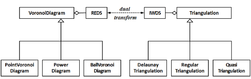
Figure 11: Class design of the topology structures in MGOS. The dual transformation between REDS and IWDS facilitates those between all three types of Voronoi diagrams and all three types of triangulations.

Fig. 12 shows the details of REDS and IWDS. REDS in Fig. 12(a) stores the topology of the Voronoi diagram and has the class definitions of the topological entities of the Voronoi diagram: cells, faces, edges, and vertices which are denoted by VD_Cell, VD_Face, VD_Edge, and VD_Vertex. Each cell points to $|F|$ faces which define its boundary and each face points to two incident cells. Each vertex points to its four incident edges and each edge points to its two vertices. In the ordinary Voronoi diagram of points, or power diagram, a face has only one loop of edges which defines the boundary of the face (thus called the outer-loop). In the Voronoi diagram $\mathcal{VD}$ of 3D spheres, however, a face may have an inner-loop(s) in addition to the outer-loop where each corresponds to an edge-graph disconnected from that of the rest of the entire Voronoi diagram. This observation is reflected in the pointer from VD_Face to Loop. In the Voronoi diagram, an edge has three, and only three, incident faces and in REDS, each edge has three copies of its replica called partial edges PartialEdge where each participates in the loop of an incident face. The three partial edges are connected in a circular manner in the counterclockwise orientation around the directed VD_Edge and in our implementation, each VD_Edge points one of the partial edges.

IWDS in Fig. 12(b) stores the topology of the quasi-triangulation and has the class definitions of topological entities of cells, faces, edges, and vertices of the quasi-triangulation which are denoted by QT_Cell, QT_Face, QT_Edge, and QT_Vertex. Note that the data structure is designed for the quasi-triangulation because the other two triangulations are its special cases. In the quasi-triangulation, a cell has four faces and each face has two incident cells; A face has three edges and an edge has a set of $1+N_{small-world}$ pointers where each of the $N_{small-world}$ pointers indicate the entrance to a small-world which corresponds to an inner loop of QT_Face. An edge has two vertices and a cell has four vertices. A vertex has a pointer to an incident edge and one to an incident cell.

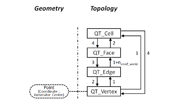
Figure 12: Data structure of REDS and IWDS. (a) REDS, (b) IWDS.

7 Conclusions

Despite the importance of the geometry of atomic arrangements in many fields, no general framework of mathematical/computational theory for the geometry of atomic arrangement exists. In this paper, we introduce “Molecular Geometry (MG)” as a theoretical framework and “MG Operating System (MGOS)” as a middleware to implement the MG theory.

We assert that MG/MGOS will free researchers from time-consuming and error-prone tasks of developing and implementing highly sophisticated and complex algorithms of a geometrical nature for molecular structure studies so that they can focus more on fundamental research issues of their own. We anticipate that MG/MGOS will facilitate the enhancement of many popular programs and the development of many new programs from diverse communities of computational science and engineering working on the arrangement of spherical objects, including molecules.

The challenge remaining is how to identify the set of primitive transformations for geometrization so as to cover as diverse a range of applications and as accurate a set of solutions as possible. The extensions of MGOS to dynamic situations for moving atoms and to big models such as geometric cell models are also a challenge. We envision that MG and MGOS together will eventually establish a new paradigm for the computational study of atomic arrangements for both organic and inorganic molecules. MGOS is freely available at http://voronoi.hanyang.ac.kr/software/mgos/.

Appendix 1. 300 Test PDB Models

Table 1: The 300 tested PDB models.

1AA2	1ARL	1BWW	1C26	1CEX	1CT4	1D2K	1D4T	1DC9	1DKL
1DQ0	1DQZ	1E2T	1EAI	1EDQ	1EKG	1EQP	1ES9	1EUM	1EY4
1EZG	1F2V	1F41	1F46	1F60	1FA8	1FCQ	1FHL	1FQN	1GCP
1HM5	1I2T	1I8K	1IFV	1ILW	1IOK	1IS5	1IXV	1IZ6	1IZ9
1J27	1J2W	1JEZ	1JLN	1JVW	1JYH	1K1B	1K5A	1KF5	1KPK
1KYF	1KZ1	1L3K	1L7A	1L7J	1LB1	1LBW	1LF1	1LHP	1LN4
1LRZ	1LU9	1LW1	1LZ1	1M0Z	1M4R	1M5S	1M9X	1MHN	1MN6
1MN8	1NKD	1NLB	1NR2	1NWA	1ORJ	1OTV	1P3C	1PM4	1Q5Z
1QB5	1QKD	1QP1	1QQ1	1QXH	1QZN	1R0M	1R0V	1R1R	1R1W
1R29	1R2T	1R3R	1R4B	1R5Z	1R8O	1RAV	1RC9	1RH9	1RL0
1RXZ	1S4F	1SAU	1SH5	1SNZ	1SRV	1SWH	1SYQ	1T45	1T4Q
1T5O	1T6F	1T7N	1TM2	1TP6	1TQG	1TZQ	1U07	1U3Y	1UC7
1UCS	1UGQ	1ULK	1ULN	1ULQ	1VDH	1VDK	1VDQ	1VES	1VFQ
1VRX	1WLG	1WM3	1WU3	1WU9	1WX0	1WYT	1X13	1X25	1X7F
1X91	1XG2	1XH3	1XIX	1XL9	1XMB	1XMP	1XN2	1XO7	1XQO
1XWG	1Y0M	1Y2T	1Y7Y	1Y9U	1YBO	1YCK	1YM5	1YOY	1YP5
1YPF	1YVI	1Z96	1ZCF	1ZEQ	1ZG4	1ZKR	1ZLB	1ZLM	1ZPW
1ZRS	1ZS3	1ZVT	1ZWS	1ZX6	1ZYE	1ZZG	1ZZK	2A28	2A4V
2A8F	2AB0	2AHE	2AQ1	2B0J	2B1K	2B3M	2B43	2BCM	2BMA
2CAR	2CWC	2CWL	2CYG	2D7T	2DEP	2DFU	2DHH	2DPO	2DU7
2E3Z	2ECE	2EKC	2EKY	2EO8	2EP5	2EQ5	2ERF	2ERW	2ESK
2ESN	2ET6	2F51	2F6L	2F82	2FBQ	2FC3	2FHZ	2FIQ	2FN9
2FP8	2FTS	2FU0	2G5X	2G7O	2G85	2GAI	2GAS	2GBJ	2GDG
2GDN	2GE7	2GFB	2GG4	2GGK	2GGV	2GMY	2GOI	2GPO	2GTD
2GUV	2H2R	2H3L	2H8O	2HK2	2HWX	2HWZ	2I1S	2I3F	2I49
2I6V	2IC6	2IG8	2IGD	2IPB	2IPR	2J0N	2J69	2NLS	2NM0
2NVW	2O37	2O70	2O7H	2OBI	2OEB	2OL7	2ON7	2OP6	2P19
2P2C	2PET	2PLQ	2PLU	2PN7	2QDN	2QE7	2QV3	2R57	2R6U
2TMG	2UX2	2V0V	2VHI	2VL0	2YZ1	2Z43	2Z5E	3B7H	3B8N
3BB7	3BG1	3BHS	3BIP	3BJV	3BTU	3BXY	3CB4	3PVA	4EUG

Appendix 2. APIs of MGOS

MGOS has several useful API-commands which can be conveniently called from user-created application programs. Some important current APIs are shown below. The name of each command explains its task.

• Basic API : Five APIs

  1. clear()

  2. load_atoms( atoms )

  3. preprocess()

  4. get_all_atoms()

  5. number_of_atoms()
     

• Entity locator API (proximity query I) : Twelve APIs

  1. find_boundary_atoms_in_van_der_Waals_model()

  2. find_buried_atoms_in_van_der_Waals_model()

  3. find_first_order_neighbor_atoms_in_van_der_Waals_model( atom )

  4. find_first_order_neighbor_atoms_in_van_der_Waals_model( atomArrangement )

  5. find_second_order_neighbor_atoms_in_van_der_Waals_model( atom )

  6. find_second_order_neighbor_atoms_in_van_der_Waals_model( atomArrangement )

  7. find_boundary_atoms_in_Lee_Richards_model( solventProbeRadius )

  8. find_buried_atoms_in_Lee_Richards_model( solventProbeRadius )

  9. find_first_order_neighbor_atoms_in_Lee_Richards_model( solventProbeRadius, atom )

  10. find_first_order_neighbor_atoms_in_Lee_Richards_model( solventProbeRadius, atomArrangement )

  11. find_second_order_neighbor_atoms_in_Lee_Richards_model( solventProbeRadius, atom )

  12. find_second_order_neighbor_atoms_in_Lee_Richards_model( solventProbeRadius, atomArrangement )
      

• Entity verifier API (proximity query II) : Six APIs

  1. is_atom_on_boundary_of_van_der_Waals_model( atom )

  2. is_buried_atom_van_der_Waals_model( atom )

  3. are_atoms_adjacent_in_van_der_Waals_model( atom1, atom2 )

  4. is_atom_on_boundary_of_Lee_Richards_model( solventProbeRadius, atom )

  5. is_buried_atom_of_Lee_Richards_model( solventProbeRadius, atom )

  6. are_atoms_adjacent_in_Lee_Richards_model( solventProbeRadius, atom1, atom2 )
     

• Entity counter API : Twelve APIs

  1. number_of_boundary_atoms_in_van_der_Waals_model()

  2. number_of_buried_atoms_in_van_der_Waals_model()

  3. number_of_first_order_neighbor_atoms_in_van_der_Waals_model( atom )

  4. number_of_second_order_neighbor_atoms_in_van_der_Waals_model( atom )

  5. number_of_first_order_neighbor_atoms_in_van_der_Waals_model( atomArrangement )

  6. number_of_second_order_neighbor_atoms_in_van_der_Waals_model( atomArrangement )

  7. number_of_boundary_atoms_in_Lee_Richards_model( solventProbeRadius )

  8. number_of_buried_atoms_in_Lee_Richards_model( solventProbeRadius )

  9. number_of_first_order_neighbor_atoms_in_Lee_Richards_model( solventProbeRadius, atom )

  10. number_of_second_order_neighbor_atoms_in_Lee_Richards_model( solventProbeRadius, atom )

  11. number_of_first_order_neighbor_atoms_in_Lee_Richards_model( solventProbeRadius, atomArrangement )

  12. number_of_second_order_neighbor_atoms_in_Lee_Richards_model( solventProbeRadius, atomArrangement )
      

• Property evaluator API (geometric computation) : Ten APIs

  1. compute_volume_of_van_der_Waals_model()

  2. compute_area_of_van_der_Waals_model()

  3. compute_volume_and_area_of_van_der_Waals_model()

  4. compute_voids_of_van_der_Waals_model()

  5. compute_volume_of_Lee_Richards_model( solventProbeRadius )

  6. compute_area_of_Lee_Richards_model( solventProbeRadius )

  7. compute_volume_and_area_of_Lee_Richards_model( solventProbeRadius )

  8. compute_voids_of_Lee_Richards_model( solventProbeRadius )

  9. compute_channels( solventProbeRadius, gateSize )

  10. compute_pockets( ligandSize, solventProbeRadius )

References

- [1] D. Morgan, A. V. der Ven, G. Ceder, Li conductivity in (m = mn, fe, co, ni) olivine materials, Electrochemical and Solid-State Letters 7 (2) (2004) A30–A32.
- [2] H. Li, M. Eddaoudi, M. O’Keeffe, O. M. Yaghi, Design and synthesis of an exceptionally stable and highly porous metal-organic framework, Nature 402 (1999) 276–279.
- [3] H. Furukawa, N. Ko, Y. B. Go, N. Aratani, S. B. Choi, E. Choi, A. Yazaydin, R. Q.Snurr, M. OKeeffe, Ultrahigh porosity in metal-organic frameworks, Science 329 (5990) (2010) 424–428.
- [4] C. Chothia, Hydrophobic bonding and accessible surface area in proteins, Nature 248 (1974) 338–339.
- [5] M. L. Connolly, Solvent-accessible surfaces of proteins and nucleic acids, Science 221 (1983) 709–713.
- [6] S. J. Hubbard, K.-H. Gross, P. Argos, Intramolecular cavities in globular proteins, Protein Engineering 7 (5) (1994) 613–626.
- [7] D. A. Doyle, joao Morais Cabral, R. A. Pfuetzer, A. Kuo, J. M. Gulbis, S. L. Cohan, B. T. Chait, R. Mackinnon, The structure of the potassium channel: Molecular basis of k conduction and selectivity, Science 280 (1998) 69–77.
- [8] A. Yonath, K. R. Leonard, H. G. Wittmann, A tunnel in the large ribosomal subunit revealed by three-dimensional image reconstruction, Science 236 (4803) (1987) 813–816.
- [9] X. Liu, E. C.Theil, Ferritins: Dynamic management of biological iron oxygen chemistry, Accounts of Chemical Research 38 (3) (2005) 167–175.
- [10] C. H. Park, S. Y. Lee, D. S. Hwang, D. W. Shin, D. H. Cho, K. H. Lee, T.-W. Kim, T.-W. Kim, M. Lee, D.-S. Kim, C. M. Doherty, A. W. Thornton, A. J. Hill, M. D. Guiver, Y. M. Lee, Nano-crack regulated self-humidifying membranes, Nature 532 (7600) (2016) 480–483.
- [11] T. Gerling, K. F. Wagenbauer, A. M. Neuner, H. Dietz, Dynamic dna devices and assemblies formed by shape-complementary, non–base pairing 3d components, Science 347 (6229) (2015) 1446–1452.
- [12] M. N. O’Brien, M. R. Jones, B. Lee, C. A. Mirkin, Anisotropic nanoparticle complementarity in DNA-mediated co-crystallization, Nature Materials 14 (2015) 833–839.
- [13] E. Fischer, Synthesen in der zuckergruppe, Berichte der deutschen chemischen Gesellschaft 23 (2) (1890) 2114–2141.
- [14] J. Daniel E. Koshland, Application of a theory of enzyme specificity to protein synthesis, Proceedings of National Academy of Science 44 (1958) 98–104.
- [15] A. Shrake, J. A. Rupley, Environment and exposure to solvent of protein atoms. lysozyme and insulin, Journal of Molecular Biology 79 (2) (1973) 351–371.
- [16] G. J. Kleywegt, T. A. Jones, Detection, delineation, measurement and display of cavities in macromolecular structures, Acta Crystallographica Section D 50 (1994) 178–185.
- [17] F. M. Richards, Areas, volumes, packing, and protein structure, Annual Review of Biophysics and Bioengineering 6 (1977) 151–176.
- [18] J.-K. Kim, Y. Cho, R. A. Laskowski, S. E. Ryu, K. Sugihara, D.-S. Kim, BetaVoid: molecular voids via beta-complexes and Voronoi diagrams, Proteins: Structure, Functions, and Bioinformatics 82 (9) (2014) 1829–1849.
- [19] J.-K. Kim, Y. Cho, M. Lee, R. A. Laskowski, S. E. Ryu, K. Sugihara, D.-S. Kim, BetaCavityWeb: a webserver for molecular voids and channels, Nucleic Acids Research 43 (W1) (2015) W413–W418.
- [20] RCSB Protein Data Bank, http://www.rcsb.org/pdb/.
- [21] M. Vlassi, G. Cesareni, M. Kokkinidis, A correlation between the loss of hydrophobic core packing interactions and protein stability, Journal of Molecular Biology 285 (2) (1999) 817–827.
- [22] S. Horiuchi, H. Tanaka, E. Sakuda, Y. Arikawa, K. Umakoshi, Encapsulation condition dependent photophysical properties of polypyridyl ru(ii) complexes within a hydrogen-bonded capsule, Dalton Transactions 48 (2019) 5156–5160.
- [23] A. Shimada, M. Kubo, S. Baba, K. Yamashita, K. Hirata, G. Ueno, T. Nomura, T. Kimura, K. Shinzawa-Itoh, J. Baba, K. Hatano, Y. Eto, A. Miyamoto, H. Murakami, T. Kumasaka, S. Owada, K. Tono, M. Yabashi, Y. Yamaguchi, S. Yanagisawa, M. Sakaguchi, T. Ogura, R. Komiya, J. Yan, E. Yamashita, M. Yamamoto, H. Ago, S. Yoshikawa, T. Tsukihara, A nanosecond time-resolved XFEL analysis of structural changes associated with CO release from cytochrome C oxidase, Science Advances 3 (7) (2017) 1–12.
- [24] L. Ducassoua, L. Dhers, G. Jonasson, N. Pietrancosta, J.-L. Boucher, D. Mansuy, F. André, Membrane-bound human orphan cytochrome P450 2U1: Sequence singularities, construction of a full 3d model, and substrate docking, Biochimie 140 (2017) 166–175.
- [25] T. Molcan, S. Swigonska, K. Orlowska, K. Myszczynski, A. Nynca, A. Sadowska, M. Ruszkowska, J. P. Jastrzebski, R. E. Ciereszko, Structural-functional adaptations of porcine CYP1A1 to metabolize polychlorinated dibenzo--dioxins, Chemosphere 168 (2017) 205–216.
- [26] F. J. Rizzuto, J. R. Nitschke, Stereochemical plasticity modulates cooperative binding in a cuboctahedron, Nature Chemistry 9 (2017) 903–908.
- [27] G. Markiewicz, A. Jenczak, M. Kołodziejski, J. J. Holstein, J. K. M. Sanders, A. R. Stefankiewicz, Selective encapsulation by a robust octameric nanospheroid held together by 48 cooperative hydrogen bonds, Nature Communications 8 (15109) (2017) 1–8.
- [28] V. Chaptal, F. Delolme, A. Kilburg, S. Magnard, C. Montigny, M. Picard, C. Prier, L. Monticelli, O. Bornert, M. Agez, S. Ravaud, C. Orelle, R. Wagner, A. Jawhari, I. Broutin, E. Pebay-Peyroula, J.-M. Jault, H. R. Kaback, M. le Maire, P. Falson, Quantification of detergents complexed with membrane proteins, Scientific Reports 7 (41751) (2017) 1–12.
- [29] L. Zhang, J. B. Bailey, R. H. Subramanian, A. Groisman, F. A. Tezcan, Hyperexpandable, self-healing macromolecular crystals with integrated polymer networks, Nature 557 (2018) 86–91.
- [30] S. Kitanovic, C. A. Marks-Fife, Q. A. Parkes, P. R. Wilderman, J. R. Halpert, M. D. Dearing, Cytochrome p450 2b diversity in a dietary specialist—the red tree vole (arborimus longicaudus), Journal of Mammalogy 99 (3) (2018) 578–585.
- [31] T. Nagae, H. Yamada, N. Watanabe, High-pressure protein crystal structure analysis of escherichia coli dihydrofolate reductase complexed with folate and nadp+, Acta Crystallographica Section D 74 (2018) 895–905.
- [32] B. Htan, D. Luo, C. Ma, J. Zhang, Q. Gan, Water-trapping of metal-organic cages with endohedral variation, Crystal Growth & Design 19 (5) (2019) 2862–2868.
- [33] A. Chakravorty, E. Gallicchio, A grid‐based algorithm in conjunction with a gaussian‐based model of atoms for describing molecular geometry, Computational Chemistry 40 (12) (2019) 1290–1304.
- [34] D.-S. Kim, Y. Cho, D. Kim, Euclidean Voronoi diagram of 3D balls and its computation via tracing edges, Computer-Aided Design 37 (13) (2005) 1412–1424.
- [35] D.-S. Kim, D. Kim, Y. Cho, K. Sugihara, Quasi-triangulation and interworld data structure in three dimensions, Computer-Aided Design 38 (7) (2006) 808–819.
- [36] D.-S. Kim, Y. Cho, K. Sugihara, Quasi-worlds and quasi-operators on quasi-triangulations, Computer-Aided Design 42 (10) (2010) 874–888.
- [37] D.-S. Kim, Y. Cho, K. Sugihara, J. Ryu, D. Kim, Three-dimensional beta-shapes and beta-complexes via quasi-triangulation, Computer-Aided Design 42 (10) (2010) 911–929.
- [38] J. A. Le Bel, On the relations which exist between the atomic formulas of organic compounds and the rotatory power of their solutions (orig. publ. 1874), in: G. M. Richardson (Ed.), The Foundations of Stereochemistry, 1901, pp. 47–59, the Richardson translations have been reprinted in Benfey, O.T., Ed. Classics in the Theory of Chemical Combination; Dover: New.
- [39] J. H. van’t Hoff, A suggestion looking to the extension into space of the structural formulas at present used in chemistry, and a note upon the relations between the optical activity and the chemical constitution of organic compounds (orig. publ. 1874), in: G. M. Richardson (Ed.), The Foundations of Stereochemistry, 1901, pp. 66–73.
- [40] R. B. Grossman, Van’t hoff, le bel, and the development of stereochemistry: A reassessment, Journal of chemical education 66 (1) (1989) 30–33.
- [41] N. Sidgwick, H. Powell, Bakerian lecture. stereochemical types and valency groups, in: Proceedings of the Royal Society A: Mathematical, Physical & Engineering Sciences, Vol. 176, 1940.
- [42] R. J. Gillespie, Molecular Geometry, Van Nostrand Reinhold, 1972.
- [43] R. J. Gillespie, R. S. Nyholm, Inorganic stereochemistry, Quarterly Reviews, Chemical Society 11 (4) (1957) 339–380.
- [44] R. J. Gillespie, The valence-shell electron-pair repulsion (VSEPR) theory of directed valency, Journal of chemical education 40 (6) (1963) 295–301.
- [45] R. Gillespie, Electron correlation and molecular shape, Canadian Journal of Chemistry 38 (1960) 818–826.
- [46] E. Fischer, Syntheses in the purine and sugar group, Nobel Lectures in Chemistry 1901-1921, Elsevier, Amsterdam, 1966.
- [47] F. Crick, The packing of a-Helices: Simple coiled-coils, Acta Crystallographica 6 (1953) 689–697.
- [48] J. Daniel E. Koshland, Correlation of structure and function in enzyme action, Science 142 (3599) (1963) 1533–1541.
- [49] J. Daniel E. Koshland, The key-lock theory and the induced fit theory, Angewandte Chemie International Edition 33 (1994) 2375–2378.
- [50] J. C. Kendrew, R. E. Dickerson, B. E. Strandberg, R. G. Hart, D. R. Davies, Structure of myoglobin: A three-dimensional fourier synthesis at 2 å. resolution, Nature 185 (4711) (1960) 422–427.
- [51] B. Lee, F. M. Richards, The interpretation of protein structures: Estimation of static accessibility, Journal of Molecular Biology 55 (1971) 379–400.
- [52] C. Chothia, Structural invariants in protein folding, Nature 254 (27) (1975) 304–308.
- [53] F. M. Richards, The interpretation of protein structures: Total volume, group volume distributions and packing density, Journal of Molecular Biology 82 (1974) 1–14.
- [54] R. A. Laskowski, M. W. MacArthur, D. S. Moss, J. M. Thornton, PROCHECK: a program to check the stereochemical quality of protein structures, Journal of Applied Crystallography 26 (1993) 283–291.
- [55] V. B. Chen, W. B. A. III, J. J. Headd, D. A. Keedy, R. M. Immormino, G. J. Kapral, L. W. Murray, J. S. Richardson, D. C. Richardson, MolProbity: All-atom structure validation for macromolecular crystallography, Acta Crystallographica Section D: Biological Crystallography 66 (1) (2010) 12–21.
- [56] I. W. Davis, A. Leaver-Fay, V. B. Chen, J. N. Block, G. J. Kapral, X. Wang, L. W. Murray, W. B. A. III, J. Snoeyink, J. S. Richardson, D. C. Richardson, MolProbity: all-atom contacts and structure validation for proteins and nucleic acids, Nucleic Acids Research 35 (2007) W375–383.
- [57] W.-H. Shin, J.-K. Kim, D.-S. Kim, C. Seok, GalaxyDock2: protein-ligand docking using beta-complex and global optimization, Journal of Computational Chemistry 34 (30) (2013) 2647–2656.
- [58] J. Ryu, M. Lee, J. cha, R. A. Laskowski, S. E. Ryu, D.-S. Kim, BetaSCPWeb: side-chain prediction for protein structures using voronoi diagrams and geometry prioritization, Nucleic Acids Research 44 (W1) (2016) W416–W423.
- [59] A. Bondi, van der Waals volumes and radii, Journal of Physical Chemistry 68 (1964) 441–451.
- [60] J. C. Slater, Atomic radii in crystals, Journal of Chemical Physics 41 (10) (1964) 3199–3204.
- [61] W. C. Still, A. Tempczyk, R. C. Hawley, T. Hendrickson, Semianalytical treatment of solvation for molecular mechanics and dynamics, Journal of the American Chemical Society 112 (16) (1990) 6127–6129.
- [62] A. Onufriev, D. Bashford, D. A.Case, Exploring protein native states and large-scale conformational changes with a modified generalized born model, Proteins: Structure, Function, and Bioinformatics 55 (2) (2004) 383–394.
- [63] S. W. Lockless, M. Zhou, R. MacKinnon, Structural and thermodynamic properties of selective ion binding in a channel, PLOS BIOLOGY 5 (5) (2007) 1079–1088.
- [64] J. Tsai, R. Taylor, C. Chothia, M. Gerstein, The packing density in proteins: Standard radii and volumes, Journal of Molecular Biology 290 (1999) 253–266.
- [65] J. D. Bernal, J. L. Finney, Random close-packed hard-sphere model II. Geometry of random packing of hard spheres, Discussions of the Faraday Society 43 (1967) 62–69.
- [66] A. Okabe, B. Boots, K. Sugihara, S. N. Chiu, Spatial Tessellations: Concepts and Applications of Voronoi Diagrams, 2nd Edition, John Wiley & Sons, Chichester, 1999.
- [67] K. Lee, Principles of CAD/CAM/CAE Systems, Addison-Wesley, Boston, 1999.