Nuclear effective field theory: status and perspectives

Abstract

The nuclear physics landscape has been redesigned as a sequence of effective field theories (EFTs) connected to the Standard Model through symmetries and lattice simulations of Quantum Chromodynamics (QCD). EFTs in this sequence are expansions around different low-energy limits of QCD, each with its own characteristics, scales, and ranges of applicability regarding energy and number of nucleons. We review each of the three main nuclear EFTs—Chiral, Pionless, Halo/Cluster—highlighting their similarities, differences, and connections. In doing so, we survey the structural properties and reactions of nuclei that have been derived from the ab initio solution of the few- and many-body problem built upon EFT input.

I Introduction

The problem of obtaining the properties of atomic nuclei from the interactions among the constituent nucleons has been central to nuclear physics since its inception. Attempts to derive nuclear forces and currents from the exchange of mesons—in particular the lightest meson, the pion—were derailed in the 1950s by a lack of renormalizability, that is, by an uncontrolled sensitivity to physics at short distances. The rise in the 1970s of a renormalizable theory of the strong interactions, Quantum Chromodynamics (QCD), did not immediately offer a path forward: because QCD—formulated in terms of quarks and gluons—is nonperturbative for processes characterized by external momenta $Q\stackrel{{\scriptstyle<}}{{{}_{\sim}}}M_{\text{QCD}}\sim 1\leavevmode\nobreak\ \mathrm{GeV}$, it is very difficult to calculate the properties of hadrons and nuclei, a problem that becomes more severe as the number $A$ of nucleons increases. Yet, a precise and accurate description of nuclei is crucial for the transition from the perturbative regime of the Standard Model to the atomic domain and beyond, governed by Quantum Electrodynamics (QED) and its small fine-structure constant. Examples relying on input from nuclear physics include tests of fundamental symmetries (such as neutrinoless double-beta decay to probe lepton number violation) and reactions in astrophysical environments.

About a quarter of a century ago effective field theories (EFTs) entered nuclear physics Weinberg (1990); Rho (1991); Weinberg (1991); Ordóñez and van Kolck (1992); Weinberg (1992); van Kolck (1993). EFTs had been developed in particle and condensed-matter physics to deal with systems containing multiple momentum scales. An EFT captures the most general dynamics among low-energy degrees of freedom that is consistent with some assumed symmetries. In nuclear physics, where the symmetries of QCD are known, an EFT provides a realization of QCD in terms of hadrons instead of quarks and gluons. All the details of the QCD dynamics at short distances are encoded in the EFT interaction strengths (“Wilson coefficients” or “low-energy constants”). Scattering amplitudes (and their poles representing bound states and resonances) are calculated as expansions in $Q/M_{\text{hi}}$ and $M_{\text{lo}}/M_{\text{hi}}$, with $M_{\text{hi}}$ the momentum scale where the EFT breaks down and $M_{\text{lo}}$ standing for low-energy scales of physics we want to capture. An EFT is renormalizable in the sense that at each order in the expansion the sensitivity to unaccounted short-distance physics is small, that is, of relative $\mathcal{O}(Q/M_{\text{hi}},M_{\text{lo}}/M_{\text{hi}})$. EFTs opened the door to a description of nuclear phenomena with systematic error estimates.

EFTs have, in fact, revolutionized nuclear physics. Most of the “ab initio” studies of nuclear structure—based on the explicit solution of the Schrödinger equation or its equivalents—are now carried out with potentials inspired by EFT. A host of nuclear properties has been predicted or postdicted from two- and three-nucleon forces, and one- and two-nucleon currents with low-energy constants were determined from $A\leq 3$ experimental data. In parallel, starting with Beane et al. (2006), fully dynamical simulations of QCD on a discretized and boxed spacetime have been able to access some $A\leq 4$ properties. Matching an EFT to results from lattice QCD (LQCD), and not just to experiment, allows for a determination of the low-energy constants. EFTs thus build a bridge between QCD and nuclear structure and reactions.

Historically the first nuclear EFT was Chiral (or Pionful) EFT Weinberg (1990); Rho (1991); Weinberg (1991); Ordóñez and van Kolck (1992); Weinberg (1992); van Kolck (1993), which is designed for momenta of the order of the pion mass. In addition to nucleons, it includes explicit pions, whose interactions are constrained by an approximate global symmetry of QCD, the chiral symmetry of independent flavor rotations of left- and right-handed quarks. Chiral EFT generalizes a popular hadronic EFT, Chiral Perturbation Theory Weinberg (1979); Gasser and Leutwyler (1984, 1985), to $A\geq 2$. Despite its phenomenological successes, Chiral EFT has proven to be extremely challenging to renormalize due to the singularity of the dominant interactions, which have to be treated nonperturbatively in order to produce bound states and resonances, i.e., nuclei. Originally conceived as a renormalization playground, a simpler EFT—Pionless (or Contact) EFT—focuses on momenta below the pion mass Bedaque and van Kolck (1998); van Kolck (1997); Kaplan et al. (1998a); Bedaque et al. (1998); Kaplan et al. (1998b); van Kolck (1999b); Birse et al. (1999). This EFT, whose renormalization is relatively well understood, is constrained only by QCD spacetime symmetries. It exhibits a high degree of universality, and except for the degrees of freedom it is formally identical to other EFTs where all interactions are of short range. Light nuclei are well described within the same framework that has been successful for atomic systems with large scattering lengths (for example, near a Feshbach resonance) Braaten and Hammer (2006). A variant of this EFT, Halo/Cluster EFT, has been applied Bertulani et al. (2002); Bedaque et al. (2003a) to bound states and reactions involving halo and cluster nuclei, characterized by such low energies that one or more tight clusters of nucleons can be treated as elementary degrees of freedom.

No doubt there are “more effective” EFTs to be discovered for larger nuclei. In fact, a description of rotational and vibrational bands in heavy nuclei has been initiated by Papenbrock (2011), with successful applications to different nuclei and processes Papenbrock and Weidenmueller (2014); Coello Pérez and Papenbrock (2015, 2016); Coello Pérez et al. (2018a, b); Chen et al. (2018, 2019). These recent developments extend the EFT paradigm to generalized degrees of freedom that capture the low-energy physics of deformed nuclei.

Here we present a summary of the main ideas, achievements, and prospects for the nuclear EFTs formulated in terms of nucleons and clusters thereof. These theories can be thought of as a tower of EFTs at successively lower $M_{\text{hi}}$, starting at $M_{\text{QCD}}$. Our emphasis is not on phenomenology, but on the conceptual similarities and differences among Chiral, Pionless, and Halo/Cluster EFTs. Our hope is that a focused approach will stimulate a reformulation of our understanding of heavy nuclei, just as these EFTs have shed new light on the structure and reactions of light nuclei.

In the remainder of this section some common aspects of nuclear EFTs are presented. Each of the three following sections deal with one nuclear EFT. In Sec. V we address the connection between these EFTs and QCD, as well as broader applications. We conclude in Sec. VI. We use throughout units such that $\hbar=1$ and $c=1$.

I.1 Nuclei from the perspective of QCD

As an $SU(3)_{\rm c}$ gauge theory of colored quarks and gluons, QCD is characterized by a coupling constant $g_{s}$ that becomes strong at low momenta. The fact that most hadron masses are about $1\leavevmode\nobreak\ \mathrm{GeV}$ or higher—for example, the nucleon mass $m_{N}\simeq 940$ MeV—reveals that nonperturbative QCD phenomena are associated with a mass scale $M_{\text{QCD}}\sim 1\leavevmode\nobreak\ \mathrm{GeV}$. The EFT at the scale of a few GeV includes not only strong interactions, but also electroweak and even weaker interactions. In contrast to most textbooks, for convenience we refer to this EFT, which is our starting point, simply as QCD. Focusing on the two lightest (up and down) quarks most relevant to nuclear physics, the QCD Lagrangian is written in terms of quark $q=(u\;d)^{T}$, gluon $G_{\mu}$ and photon $A_{\mu}$ fields as

$$\mathcal{L}_{\text{QCD}}=\bar{q}\left[\mathrm{i}\gamma^{\mu}\left(\partial_{\mu}+\mathrm{i}g_{s}G_{\mu}+\mathrm{i}eQA_{\mu}\right)+\bar{m}\left(1-\varepsilon\tau_{3}\right)\right]q\\ \hbox{}-\frac{1}{2}{\rm Tr}\;G_{\mu\nu}G^{\mu\nu}-\frac{1}{4}F_{\mu\nu}F^{\mu\nu}+{\cdots},$$ (3)

where $\gamma_{\mu}$ and $\tau_{i}$ are the Dirac and Pauli matrices, and $G_{\mu\nu}$ and $F_{\mu\nu}$ are the gauge and photon field strengths. Neglecting the “$\cdots$”, which include for example weak interactions, the only parameters in QCD are the quark masses and electromagnetic charges. We can express quark masses in terms of the common mass $\bar{m}=(m_{u}+m_{d})/2\sim 5\leavevmode\nobreak\ \mathrm{MeV}$ and of the relative mass splitting $\varepsilon=(m_{d}-m_{u})/(m_{u}+m_{d})\sim 1/3$. The quark charges are fractions $Q={\text{diag}}(2/3,-1/3)$ of the proton charge $e=\sqrt{4\pi\alpha}\sim 1/3$.

Below $M_{\text{QCD}}$, QCD is best represented as a theory of colorless hadrons, where $SU(3)_{\mathrm{c}}$ is realized trivially. An important role is played by pions, which arise as pseudo-Goldstone bosons from the spontaneous breaking of approximate $SU(2)_{\mathrm{L}}\times SU(2)_{\mathrm{R}}$ chiral symmetry down to its vector subgroup $SU(2)_{\mathrm{V}}$ of isospin. In the chiral limit $\bar{m}=0$, $\varepsilon=0$ and $e=0$, chiral symmetry is exact, and pions are massless and interact purely derivatively. Away from the chiral limit, the common quark mass breaks chiral symmetry explicitly and leads to a nonzero common pion mass $m_{\pi}\simeq 140\leavevmode\nobreak\ \mathrm{MeV}$ and nonderivative pion interactions. The QCD interactions associated with $\varepsilon$ and $e$ further break isospin, and appear in relatively small quantities such as the pion mass splitting $\delta m_{\pi}^{2}=m_{\pi^{\pm}}^{2}-m_{\pi^{0}}^{2}\simeq(36\leavevmode\nobreak\ \mathrm{MeV})^{2}$ and the neutron-proton mass difference $\delta m_{N}=m_{n}-m_{p}\simeq 1.3\leavevmode\nobreak\ \mathrm{MeV}$.

A more complete understanding of the low-energy consequences of QCD can be achieved if we consider alternative realities where $\bar{m}$, $\varepsilon$, and $e$ are varied from their real-world values. So far, LQCD simulations of nuclear quantities have been carried out in the isospin-symmetry limit, where $\varepsilon=0$ and $e=0$. The only remaining QCD parameter, $\bar{m}$, can be traded for the pion mass $m_{\pi}$. Because the signal-to-noise ratio for $A$-nucleon correlation functions at large time $t$ scales as $\exp{[-A(m_{N}-3m_{\pi}/2)t]}$ Lepage (1989a); Beane et al. (2011), current simulations are limited to unphysically large $m_{\pi}$ and to small $A$. Although one can expect future simulations at smaller pion masses and more nucleons, it is more efficient to switch to an EFT description suited to the large distances involved in nuclear physics.

Years of experience suggest that nuclei can be seen as bound states or resonances made out of nucleons, or perhaps clusters of nucleons. The choice of degrees of freedom determines the range of validity $M_{\text{hi}}$ of the respective EFT. Because isospin violation is a relatively small effect for most nuclear dynamics (more so for light nuclei), we can classify nuclear EFTs by their regions of applicability according to typical momentum and pion mass, see Fig. 1. A possible estimate of the typical binding momentum, where each nucleon contributes equally to the binding energy $B_{A}$, is $Q_{A}\sim\sqrt{2m_{N}B_{A}/A}$. Nuclear saturation for large $A$ leads, at physical pion mass, to a constant $B_{A}/A\sim 10$ MeV and nuclear radii $R_{A}\sim R_{0}A^{1/3}$, where $R_{0}\sim 1.2\leavevmode\nobreak\ \mathrm{fm}$. Numerically, $Q_{A}\sim R_{0}^{-1}$ is not very different from $m_{\pi}$, and it has been assumed that Chiral EFT is best suited for typical nuclei. (In fact, we will see in Sec. IV how $B_{A}/A\sim 10$ MeV arises naturally within Chiral EFT.) At sufficiently small $Q$ and $m_{\pi}$ (i.e., below a scale $M_{N\!N}\sim 270\leavevmode\nobreak\ \mathrm{MeV}$ at the physical pion mass, see Eq. (73) for a precise definition), one expects pions to be perturbative. As $Q$ increases at fixed $m_{\pi}$, chiral-symmetric pion interactions become nonperturbative (for $A\geq 2$), and as $Q$ increases further the EFT eventually ceases to converge. As $m_{\pi}$ increases at fixed $Q$, chiral-symmetry breaking becomes more important and again the Chiral EFT expansion eventually fails. We expect that $M_{\text{hi}}\sim M_{\text{QCD}}$, but the exact breakdown values of $Q$ and $m_{\pi}$ are not well known. It seems that for $A=0$, for example, Chiral EFT (in the form of ChPT) has $M_{\text{hi}}\leq 500\leavevmode\nobreak\ \mathrm{MeV}$ Dürr (2015).

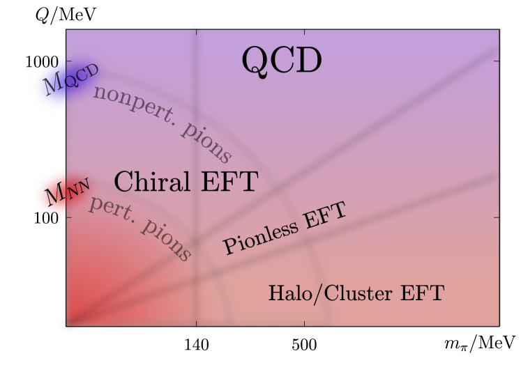
Figure 1: Landscape of nuclear EFTs in the plane of typical momentum $Q$ and pion mass $m_{\pi}$.

Light nuclei are weakly bound and radii scale differently than in the saturation regime. Pions can be treated as short-range interactions and in Pionless EFT we expect $M_{\text{hi}}\sim m_{\pi}$ at all $m_{\pi}$, including values beyond the breakdown of Chiral EFT such as in LQCD simulations to date. For $Q$ smaller than the inverse radius of a nucleus, the nucleus itself can be treated as an elementary particle in more complex systems where it appears as a sub-unit. In the Halo/Cluster EFT relevant for clusterized nuclei, $M_{\text{hi}}\sim R_{c}^{-1}$, the inverse cluster radius. Pionless and Halo/Cluster EFTs carry the information of QCD to the large distances of nuclear dynamics near the driplines.

I.2 The way of EFT

How does one ensure that a nuclear EFT reproduces QCD in the appropriate energy domain? Once degrees of freedom have been selected according to the energies of interest, one constructs the most general Lagrangian $\mathcal{L}$ involving the corresponding set of fields $\{\psi\}$, which is constrained only by the QCD symmetries,

$$\mathcal{L}=\sum_{i}c_{i}(M_{\text{lo}},M_{\text{hi}},\Lambda)\,O_{i}(\{\psi\}),$$ (4)

where the $O_{i}(\{\psi\})$ are operators that involve fields at the same spacetime point but contain an arbitrary number of derivatives, and $c_{i}(M_{\text{lo}},M_{\text{hi}},\Lambda)$ are the low-energy constants (LECs). Here $\Lambda$ denotes an arbitrary regulator parameter with dimension of mass. With $\mathcal{L}$, or the corresponding Hamiltonian, the propagation and interaction of the low-energy degrees of freedom can be calculated. The procedure might be entirely perturbative, as represented by Feynman diagrams with a finite number of loops, or partially nonperturbative, as obtained by an infinite sum of Feynman diagrams or the solution of an equivalent integral or differential equation such as, respectively, the Lippmann-Schwinger or the Schrödinger equation. In either case, the interactions are singular, which requires regularization. When the calculation can be reduced to a finite number of loops, dimensional regularization can be employed, which introduces a renormalization scale $\mu$. However, in nuclear physics we are most often faced with summing an infinite number of loops with overlapping momenta which, with present techniques, can only be made finite by the introduction, at either interaction vertices or propagators, of a momentum-regulator function $f(p/\Lambda)$ such that $f(0)=1$ and $f(x\to\infty)=0$. Here $p$ refers to the momentum of a nucleon, in which case the regulator is separable, or the transferred momentum, when the regulator is nonseparable. We can alternatively look at position space, where the nonseparable regulator is local (i.e., a function of position only) whereas the separable regulator is nonlocal.

The goal is to construct the $T$ matrix for a low-energy process as an expansion in $Q/M_{\text{hi}}<1$, schematically,

$$T(Q)=\mathcal{N}\sum_{\nu=0}^{\infty}\,\left(\frac{Q}{M_{\text{hi}}}\right)^{\!\nu}\\ \hbox{}\times F^{(\nu)}\!\left(\frac{Q}{M_{\text{lo}}},\frac{Q}{\Lambda};\gamma^{(\nu)}\!\left(\frac{M_{\text{lo}}}{M_{\text{hi}}},\frac{\Lambda}{M_{\text{hi}}}\right)\right)\,,$$ (5)

where $\mathcal{N}$ is a normalization factor, the $F^{(\nu)}$ are functions generated by the dynamics of the $\{\psi\}$, the $\gamma^{(\nu)}=\mathcal{O}(1)$ are dimensionless combinations of the $c_{i}$, and $\nu$ is a counting index. “Power counting” is the relation between $\nu$ and the interaction label $i$ in Eq. (4). While the form of the $O_{i}$ in the Lagrangian (4) depends on the choice of fields, the expansion (5) must not Chisholm (1961); Kamefuchi et al. (1961). Likewise, observables obtained from Eq. (5) must not depend on the arbitrary regularization procedure—renormalization-group (RG) invariance.

Once the expansion (5) has been achieved, one can truncate the sum at a given $\nu=\mathcal{V}$ with a small error,

$$T(Q\sim M_{\text{lo}})=T^{(\mathcal{V})}(Q,\Lambda)\left[1+\mathcal{O}\left(\frac{Q^{{\mathcal{V}}+1}}{M_{\text{hi}}^{{\mathcal{V}}+1}}\right)\right]\,.$$ (6)

Before renormalization, non-negative powers of $\Lambda$ can appear, which originate in the short-distance part of loops. The uncertainty principle ensures that such contributions cannot be separated from that of LECs. Renormalization is the procedure that fixes the cutoff dependence of the LECs so that the truncated amplitude $T^{(\mathcal{V})}(Q,\Lambda)$ satisfies approximate RG invariance,

$$\frac{\Lambda}{T^{(\mathcal{V})}(Q,\Lambda)}\frac{\mathrm{d}T^{(\mathcal{V})}(Q,\Lambda)}{\mathrm{d}\Lambda}=\mathcal{O}\left(\frac{Q^{{\mathcal{V}}+1}}{M_{\text{hi}}^{\mathcal{V}}\Lambda}\right)\,.$$ (7)

This condition ensures the error introduced by the arbitrary regularization procedure is no larger than the $Q/M_{\text{hi}}$ error stemming from the neglect of higher-order terms in Eq. (6), as long as $\Lambda\stackrel{{\scriptstyle>}}{{{}_{\sim}}}M_{\text{hi}}$. In this “modern view” of renormalization, there is no need to take the $\Lambda\to\infty$ limit Lepage (1989b). However, while in analytical calculations Eq. (7) can be verified explicitly, in numerical calculations varying the regulator parameter widely above the breakdown scale is usually the only tool available to check RG invariance. In contrast, $\Lambda<M_{\text{hi}}$ generates relatively large errors from the regularization procedure. Failure to satisfy Eq. (7) altogether means uncontrolled sensitivity to short-distance physics: results depend on the value of $\Lambda$ and on the choice of the regulator function $f(x)$, which acquires the status of a physical, model-dependent “form factor.”

After renormalization, when the contribution from momenta of the order of the large cutoff have been removed, the dominant terms in loop integrals come from momenta of $\mathcal{O}(Q)$. Counting powers of $Q$ in individual contributions to Eq. (5) is similar to determining the superficial degree of divergence of diagrams. There is, in general, also residual $\Lambda$ dependence (Eq. (7)) which can be absorbed in the LECs of higher-derivative interactions. Since shuffling short-range physics between loops and LECs does not change observables, the finite part of an LEC is expected to be set by the replacement $\Lambda\to M_{\text{hi}}$ (see, for example, Veltman (1981)), which then places an upper bound on the order these interactions appear at. The exception is when a symmetry suppresses the corresponding interaction ’t Hooft (1980). “Naturalness” assumes that all terms in the effective Lagrangian (respecting the relevant symmetries) have dimensionless coefficients of $\mathcal{O}(1)$ when the appropriate powers of $M_{\text{lo}}$ and $M_{\text{hi}}$ are factored out. Renormalization is thus a powerful tool to estimate sizes of the LECs.

This framework is a generalization of the ancient requirement of renormalizability by a finite set of parameters. If all interactions needed for Eq. (7) are present at each order, the resulting $S$ matrix incorporates the relations among QCD $S$-matrix elements demanded by symmetries, with no other assumption than an expansion in $Q/M_{\text{hi}}<1$. Every low-energy observable depends on a finite number of LECs at leading order (LO), where $\mathcal{V}=0$, a few more at next-to-leading order (NLO), where $\mathcal{V}=1$, etc. Once the LECs are determined from a finite number of data, all other observables can be pre- or postdicted with a controlled error. Traditionally the input data have been experimental, but LQCD results can now be used instead Barnea et al. (2015); Beane et al. (2015); Kirscher et al. (2015).

One of the virtues of the model independence encoded in Eq. (7) is that it provides an a priori estimate of theoretical errors. At the simplest level errors can be estimated from the higher-order terms in Eq. (6) with a guess for $M_{\text{hi}}$. A lower bound on the theoretical error is provided by cutoff variation from $M_{\text{hi}}$ to much higher values. The breakdown scale $M_{\text{hi}}$ itself can be inferred comparing the energy dependence at various orders with data Lepage (1997). Reliance on data can be minimized by using instead EFT results at different cutoffs Grießhammer (2016). Up to now both data fitting and propagation of errors have employed standard statistical analyses previously used for models. However, these methods can lead to biases because they are not particularly well suited to the a priori EFT error estimates, which typically increase with $Q$, while experimental data are sometimes more precise at higher $Q$. A comprehensive theory of EFT error analysis based on Bayesian methods is currently being developed Schindler and Phillips (2009); Furnstahl et al. (2015c, b); Wesolowski et al. (2016) with the promise of becoming the standard in the field.

I.3 Nuclear EFTs

The implementation of these ideas in nuclear physics has posed some unexpected challenges. They can be traced to the fact that at LO some interactions need to be fully iterated—or, equivalently, a dynamical equation should be solved exactly—in order to produce the bound states and resonances that we refer to as nuclei.

Nuclear EFTs typically include fields for the nucleon or clusters of nucleons. These particles have masses of $\mathcal{O}(M_{\text{QCD}})$, and the expansion (5) includes a $Q/m_{N}$ expansion around the nonrelativistic limit. Creation of virtual heavy particle-antiparticle pairs takes place at small distances $r\stackrel{{\scriptstyle<}}{{{}_{\sim}}}1/(2m_{N})$ and its effects can be absorbed in the LECs. As a consequence, a process involving $A$ heavy particles is not affected by interactions in Eq. (4) involving more than $2A$ fields associated with these heavy particles. The simplest way to incorporate the fact that the (large) particle rest energy does not play any role is to employ a “heavy field” from which the trivial evolution factor due to the rest energy is removed Jenkins and Manohar (1991a). Lorentz invariance for these fields is encoded in “reparametrization invariance” Luke and Manohar (1992). Kinetic terms reduce to the standard nonrelativistic form that respects Galilean invariance, with relativistic corrections suppressed by inverse powers of $m_{N}$ appearing at higher orders.

There is a crucial difference between $A=1$ and $A\geq 2$ processes. The former processes involve also light particles (e.g., photons) in initial and final states with momenta $Q\sim M_{\text{lo}}$. They deposit on the nucleon an energy of $\mathcal{O}(Q)$ which is larger than the recoil of $\mathcal{O}(Q^{2}/(2m_{N}))$, so that the nucleon is essentially static—deviation from the static limit can be treated as a perturbation. Intermediate states differ in energy from the initial state by an amount of $\mathcal{O}(Q)$. In contrast, there are Feynman diagrams for the $T$ matrix of an $A\geq 2$ process—whether it involves external probes or not—that include intermediate states which differ in energy from the initial state only by a small difference in nucleon kinetic energies of $\mathcal{O}(Q^{2}/(2m_{N}))$. In these “reducible” diagrams nucleons are not static, and there is an infrared (IR) enhancement relative to intermediate states for $A=1$ processes Weinberg (1991). Nucleon recoil cannot be treated perturbatively, although relativistic corrections remain small.

The “full” nuclear potential $V$ is defined as the sum of irreducible diagrams for a process involving $A$ nucleons in initial and final states. The full $T$ matrix (5) is obtained by sewing potential subdiagrams with nucleon lines representing the free $A$-body Green’s function $G$. This gives rise to the Lippmann-Schwinger equation, schematically

$$T=V+\int VGT=V+\int VGV+\cdots\,,$$ (8)

or alternatively to the Schrödinger equation and its many-body relatives. The full potential so defined involves all $A$ bodies but it includes components with $1\leq C\leq A-1$ separately connected pieces. Frequently the potential is thought of as one of these connected pieces. One thus defines the “$A$-nucleon ($AN$) potential” as the sum of diagrams with $C=1$ in the $A$-nucleon system. For $A=2$ all diagrams in the nuclear potential are connected ($C=1$), but starting at $A=3$ multiply connected diagrams appear, i.e., the full potential is made up of a sum of fewer-body potentials. Diagrams with $C=A-1$ are made out of the $2N$ potential and $A-2$ disconnected nucleon lines. Diagrams in the full potential that have $1<C<A-1$ are made of combinations of lower-$A$ potentials and disconnected nucleon lines.

In contrast to phenomenological models, all mesons with masses $\stackrel{{\scriptstyle>}}{{{}_{\sim}}}M_{\text{QCD}}$ and nucleon excitations heavier than the nucleon by the same amount can be integrated out because their effects can be captured by the LECs. As we are going to see in Sec. II, in Pionless EFT the potential consists purely of contact interactions, while in Chiral EFT pion exchanges are present as well (Sec. IV). In either case, the potential involves small transfers of energy $\mathcal{O}(Q^{2}/(2m_{N}))$, and the total exchanged four-momentum is close to the total transferred three-momentum. Dependence on the latter translates into a function of the position in coordinate space—the potential is local. Meanwhile, dependence on other nucleon momenta leads to derivatives with respect to position, i.e., the momentum operator in quantum mechanics—the potential becomes nonlocal. We expect to be able to expand the potential in momentum space analogously to Eq. (5),

$${V(Q,\Lambda)=\sum_{\mu=0}^{\infty}V^{(\mu)}(Q,\Lambda)=\tilde{\mathcal{N}}\sum_{\mu=0}^{\infty}\,\left(\frac{Q}{M_{\text{hi}}}\right)^{\!\mu}}\\ {\hbox{}\times\tilde{F}^{(\mu)}\!\left(\frac{Q}{M_{\text{lo}}};\frac{Q}{\Lambda};\tilde{\gamma}^{(\mu)}\!\left(\frac{M_{\text{lo}}}{M_{\text{hi}}},\frac{\Lambda}{M_{\text{hi}}}\right)\right)\,,}$$ (9)

where $\tilde{\mathcal{N}}$ is a normalization factor, the $\tilde{F}^{(\mu)}$ are functions obtained from irreducible diagrams, the $\tilde{\gamma}^{(\mu)}=\mathcal{O}(1)$ are dimensionless combinations of the $c_{i}$, and $\mu$ is a counting index for the potential.

When the nucleus is disturbed by low-momentum external probes (photons, leptons, perhaps pions), similar considerations apply. One can define nuclear currents (or reaction kernels) as the sum of irreducible diagrams to which the probes are attached. Again, currents involve all $A$ nucleons but include disconnected diagrams. A subtlety is that a probe can deposit an energy $\mathcal{O}(Q)$ on a nucleon line, and thus there can be purely nucleonic intermediate states in irreducible diagrams. Observables come from the sandwich of currents between wavefunctions of the initial and final states. Currents have an expansion similar to Eq. (9).

The nuclear potential and associated currents can always be defined as such intermediate quantities between $\mathcal{L}$ and $T$. We have reduced the EFT to a quantum-mechanical problem, but one in which the form of the potential and currents is determined. This is a distinct improvement over a purely phenomenological approach, particularly in what concerns the bewildering variety of many-body potentials and currents one can construct. This feature is one of the major reasons for the dominant role nuclear EFTs play nowadays in the nuclear theory community.

However, one should keep in mind that the potential and currents are not directly observable. There are important differences between Eqs. (9) and (5):

• The potential does not need to obey an equation such as (7). EFT potentials involve terms that are singular and often attractive, in the sense of diverging faster than $-1/(4m_{N}r^{2})$ as the relative position $r\to 0$. The potential would generate strong regulator dependence in Eq. (8) integrals if it did not itself depend strongly on $\Lambda$, see, e.g., a pedagogical discussion by Lepage (1997).

• Since after renormalization $\Lambda$ disappears from $T$ (apart from arbitrarily small terms),

  $$\int VGV\sim\frac{Q^{3}}{4\pi}\frac{m_{N}}{Q^{2}}V^{2}\sim\frac{m_{N}QV}{4\pi}V$$ (10)

  and the expansion (8) is in the dimensionless ratio $m_{N}QV/(4\pi)$ Bedaque and van Kolck (2002). For $Q\stackrel{{\scriptstyle>}}{{{}_{\sim}}}4\pi/(m_{N}V^{(0)})$, $F^{(0)}$ in Eq. (5) stems from an infinite iteration of the LO potential $V^{(0)}$. This is good, because nuclear bound states and resonances, as poles of $T$ matrices, can only be obtained from a nonperturbative LO.

• Equations (9) and (8) do not imply that all terms in $V$ should be treated on the same footing. One cannot immediately identify $\mu$ with $\nu$ because a term in $V$ contributes to various orders in the $T$ matrix. Higher-order $F^{(\nu>0)}$ can be obtained from $V^{(\mu>0)}$ in a distorted-wave Born expansion: $F^{(1)}$ from a single insertion of $V^{(1)}$, $F^{(2)}$ from a single insertion of $V^{(2)}$ or two insertions of $V^{(1)}$, and so on. Treating the potential truncated at a subleading order exactly—i.e., treating it as a phenomenological potential—is in general not correct from a renormalization point of view. In an expansion in $Q$, the potential gets more and more singular with increasing order. Resumming a partial subset of higher-order terms will in general not include all the LECs needed for proper renormalization.

The age-long challenge in nuclear physics has been to achieve RG invariance when some interactions are nonperturbative and yet some others can be treated as small. In an EFT, that translates into the nontrivial task of developing a power counting that guarantees Eqs. (6) and (7). In a purely perturbative context the cutoff dependence of loops can be obtained analytically. Assuming naturalness and looking at individual loop diagrams, a simple rule has been devised for the size of the LECs needed for perturbative renormalization Manohar and Georgi (1984); Georgi and Randall (1986). This “naïve dimensional analysis” (NDA) states that, for an operator $O_{i}$ in Eq. (4) with canonical dimension $D_{i}$ involving $N_{i}$ fields $\psi$,

$$c_{i}=\mathcal{O}\left(\frac{(4\pi)^{N_{i}-2}}{M_{\text{QCD}}^{D_{i}-4}}\,c_{i{\text{red}}}\right)\,,$$ (11)

where the dimensionless “reduced” LEC $c_{i\text{red}}$ is of the order of the combination of reduced QCD parameters that give rise to it. Examples for Chiral Perturbation Theory are given in Sec. IV. It is, however, not immediately obvious that NDA applies to LECs of operators involving four or more nucleon fields subject to nonperturbative renormalization, i.e., which are renormalized once LO interactions are resummed. In fact, as we are going to see below, cutoff variations in the Lippmann-Schwinger equation (8) require significant departures from NDA for contact interactions among nucleons. These departures were first understood within Pionless EFT. Its simplicity makes Pionless EFT the poster-child for nuclear EFT, and we therefore make it the start of this review.

II Pionless EFT

II.1 Motivation

At very low energies—i.e., for momenta $Q\ll m_{\pi}$—few-nucleon systems are not sensitive to the details associated with pion (or other meson) exchange. This fact makes it possible to describe such systems with short-range interactions alone (i.e. interactions of finite range or falling off at least as an exponential in the interparticle distance), an approach dating back to Bethe and his effective range expansion (ERE) for nucleon-nucleon ($N\!N$) scattering Bethe (1949)—see also related work by Bethe and Peierls (1935a, b); Fermi (1936); Schwinger (1947); Jackson and Blatt (1950). Casting this basic idea into a modern systematic framework leads directly to what has become known as Pionless EFT.

Historically, Pionless EFT emerged out of the effort to understand the renormalization of EFTs where a certain class of interactions need to be treated nonperturbatively. It had been shown by Kaplan et al. (1996), Phillips et al. (1998), and Beane et al. (1998b) that the original prescription Weinberg (1990, 1991) to extend Chiral Perturbation Theory to few-nucleon systems (discussed in Sec. IV) could not be implemented satisfying RG invariance. It turned out that there is a surprisingly rich structure of phenomena in the low-energy regime where explicit pion exchange cannot be resolved.

Formally, the pion can be regarded as “integrated out” if all other dynamical scales are much smaller than the pion mass. Consider, for example, the Yukawa potential corresponding to one-pion exchange:

$${\langle\mathbf{k}^{\prime}|V_{2N,\pi}|\mathbf{k}\rangle\propto\frac{1}{\mathbf{q}^{2}+m_{\pi}^{2}}\;,\;\mathbf{q}=\mathbf{k}^{\prime}-\mathbf{k}\,,}$$ (12)

where $\mathbf{k}$ and $\mathbf{k}^{\prime}$ are incoming and outgoing momenta of two scattered nucleons (in their center-of-mass frame). If these are both small compared to $m_{\pi}$, Eq. (12) can be expanded in $\mathbf{q}^{2}$, with the leading term being just a constant and the following terms coming with ever higher powers of $\mathbf{q}^{2}$. This shrinking of the original interaction to a point is illustrated in Fig. 2. Fourier-transforming into configuration space one obtains a series of delta functions with a growing number of derivatives. In Chiral EFT, which includes pions, analogous contact interactions represent the exchange of heavier mesons. Integrating out pions to arrive at Pionless EFT means merging unresolved pion exchange with these operators. It should be noted, however, that Chiral EFT is based on an expansion around a vanishing pion mass, whereas Pionless EFT treats $m_{\pi}$ as a large scale. As such, these two EFTs are very different—in particular, the respective LECs cannot in general be related by perturbative matching—but they are both well-defined low-energy limits of QCD.

Figure 2: Reduction of pion exchange (dashed line) to a series of contact interactions between nucleons (solid lines) for $q^{2}\ll m_{\pi}^{2}$.

In practice, one does not have to derive Pionless EFT from a more fundamental EFT by integrating out explicit pions. Instead, one can just follow the EFT paradigm and write down an effective Lagrangian, Eq. (4), with all contact interactions between nucleons that are allowed by symmetry. This restriction means that one requires invariance under “small” Lorentz boosts (Galilean boosts plus systematic relativistic corrections), rotations, isospin, and discrete symmetries like parity and time reversal, the systematic breaking of which can also be accounted for. The same EFT with other particles substituted for nucleons can describe different systems where the important dynamics takes place at distances beyond the range of the force. Some of these systems are discussed in Secs. III and V. In particular, Pionless EFT captures the universal aspects of Efimov physics Braaten and Hammer (2006).

In this section we discuss the basic features and formalism of Pionless EFT, first in the context of two-body systems (Sec. II.2) and later for a larger number of particles (Sec. II.3). Some of the outstanding issues are raised in Sec. II.4.

II.2 Weakly bound $S$-wave systems

Two very-low-energy particles, represented by a field $\psi$, can be described by an effective Lagrangian

$$\mathcal{L}=\psi^{\dagger}\left(\mathrm{i}\partial_{0}+\frac{\boldsymbol{\nabla}^{2}}{2m_{N}}\right)\psi-\frac{C_{0}}{2}(\psi^{\dagger}\psi)^{2}\\ +\frac{C_{2}}{16}\big{[}(\psi\psi)^{\dagger}\,(\psi\,(\overset{\smash{\raisebox{-1.5pt}{\tiny$\leftarrow$}}}{\boldsymbol{\nabla}}-\overset{\smash{\raisebox{-1.5pt}{\tiny$\rightarrow$}}}{\boldsymbol{\nabla}})*^{2}\psi)+\mathrm{H.c.}\big{]}+\cdots\,,$$ (13)

where $(\overset{\smash{\raisebox{-1.5pt}{\tiny$\leftarrow$}}}{\boldsymbol{\nabla}}-\overset{\smash{\raisebox{-1.5pt}{\tiny$\rightarrow$}}}{\boldsymbol{\nabla}})*=\overset{\smash{\raisebox{-1.5pt}{\tiny$\leftarrow$}}}{\boldsymbol{\nabla}}-\overset{\smash{\raisebox{-1.5pt}{\tiny$\rightarrow$}}}{\boldsymbol{\nabla}}$ is the Galilei-invariant derivative and $\mathrm{H.c.}$ denotes the Hermitian conjugate. The “$\cdots$” represent local operators with other combinations of derivatives, including relativistic corrections. Here we have adopted the notation of Hammer and Furnstahl (2000), but various forms for the Lagrangian—differing by prefactors absorbed in the low-energy constants ($C_{0}$, $C_{2}$, etc.) or choice of equivalent operators—exist in the literature. One can treat the two $N\!N$ $S$-wave channels (${}^{3}S_{1}$ or ${}^{1}S_{0}$, in the spectroscopic notation ${}^{2s+1}l_{j}$ where $l$, $s$, and $j$ denote respectively orbital angular momentum, spin, and total angular momentum) simultaneously using a nucleon field $N$ that is a doublet in spin and isospin space. We will come back to this after discussing the general features of the two-body sector on the basis of Eq. (13).

II.2.1 Two-body scattering amplitude

To fill the theory described by the effective Lagrangian (13) with physical meaning, we need to equip it with a power counting. We seek an expansion of the form (5) where $M_{\text{hi}}$ is expected to be set by the pion mass $m_{\pi}$, since pion exchange has been integrated out. In particular, we want to reproduce the ERE Bethe (1949) for the on-shell $N\!N$ scattering amplitude: [eq:T-kcot] T(k,cosθ) &= -4π$m_{N}$∑_l(2l+1)Pl(cosθ)kcotδl(k)-ik  ,
k^2l+1cotδ_l(k) = -1al + rl2k^2 + O(k^4)  , with a Legendre polynomial $P_{l}$, the scattering angle $\theta$ and energy $E=k^{2}/m_{N}$ in the center-of-mass frame, and where $\delta_{l}(k)$ is the scattering phase shift in the $l$-th partial wave, while $a_{l}$ and $r_{l}$ denote the corresponding scattering length and effective range, respectively. Here, we focus on $S$ waves with $l=0$. Higher partial waves will be discussed below.

In a “natural” scenario, the LECs $C_{2n}$ in Eq. (13) would scale with inverse powers of their mass dimension, e.g., $C_{0}\propto M_{\text{hi}}^{-1}$. (Note that an overall scaling with $1/m_{N}$ from the nonrelativistic framework is shared by all terms in the effective Lagrangian.) In this case, to lowest order $T$ would simply be given by the tree-level $C_{0}$ vertex, and we could identify $C_{0}=4\pi a_{0}/m_{N}$. However, the low-energy $N\!N$ system is not natural. From the above relation for $C_{0}$ it is immediately clear what this means here: the actual $N\!N$ scattering lengths ($a_{{}^{1}S_{0}}\simeq{-}23.7\leavevmode\nobreak\ \mathrm{fm}$ and $a_{{}^{3}S_{1}}\simeq 5.4\leavevmode\nobreak\ \mathrm{fm}$) are large compared to the pion Compton wavelength $m_{\pi}^{-1}\simeq 1.4\leavevmode\nobreak\ \mathrm{fm}$, so $C_{0}=4\pi a_{0}/m_{N}$ is incompatible with $C_{0}\propto M_{\text{hi}}^{-1}$ if one assumes $M_{\text{hi}}\sim m_{\pi}$. Turning the argument around, the perturbative expansion in $C_{0}$ has a breakdown scale set by $1/a_{0}\ll m_{\pi}$, rendering it useful only for the description of extremely low-energy $N\!N$ scattering.

The physical reason for the rapid breakdown of the perturbative expansion is that the large $N\!N$ $S$-wave scattering lengths correspond to low-energy (“shallow”) bound states (virtual, in the case of the ${}^{1}S_{0}$ channel). For example, it is well known that the deuteron binding momentum $\gamma_{d}=\sqrt{\mathstrut m_{N}B_{d}}\simeq 45.7\leavevmode\nobreak\ \mathrm{MeV}$ is given to about 30% accuracy by $1/a_{{}^{3}S_{1}}$. These states directly correspond to poles of the amplitude $T$ (located on the imaginary axis of the complex $k$ plane, or on the negative energy axis in the first or second Riemann sheet). It is clear that a (Taylor) expansion of $T$ in $k^{2}$ will only converge up to the nearest pole in any direction in the complex plane. Thus, the presence of the shallow $N\!N$ bound states limits the range for a perturbative description of $N\!N$ scattering.

A nonperturbative treatment is necessary to generate poles in $T$, since a finite sum of polynomials can never have a pole. As pointed out by Weinberg (1991), this can be achieved by “resumming” the $C_{0}$ interaction, i.e., by writing the LO amplitude as the tree-level $C_{0}$ diagram plus any number of $C_{0}$ vertices with intermediate propagation, as shown in Fig. 3 (see also a related analysis by Luke and Manohar (1997)). The result for a single generic $N\!N$ channel is

$$T^{(0)} ={C_{0}+C_{0}\,I_{0}(k)\,C_{0}+C_{0}\,I_{0}(k)\,C_{0}\,I_{0}(k)\,C_{0}+\cdots}$$

$$={\left[C_{0}^{-1}-I_{0}(k)\right]^{-1}}\,,$$ (14)

where $I_{0}$ is the two-body “bubble integral,” discussed in more detail below. Having $C_{0}$ now in the denominator means that it can be adjusted to give a pole at the desired position.

Figure 3: Bubble chain for a generic $S$-wave $N\!N$ scattering amplitude at LO from the $C_{0}$ interaction (solid circle).

II.2.2 Power counting

Of course, the power counting of the theory should be such that it actually mandates this procedure. The small inverse $N\!N$ scattering lengths introduce a genuine new low-momentum scale $M_{\text{lo}}$ (or large length $M_{\text{lo}}^{-1}$). Typically, this is referred to as “fine tuning” because the existence of this scale—at odds with the perfectly natural assumption that pion exchange should set the lowest energy scale—implies that different contributions from quarks and gluons have to combine in just the right way to produce this scenario (see Sec. V.1).

Equation (14) is nothing but Eq. (8) for a two-body potential $C_{0}$, which, from the discussion above, is enhanced by a factor $M_{\text{lo}}^{-1}$. The loops connecting two insertions of the potential contain nucleon propagators, which from Eq. (13) we read off to be

$$\mathrm{i}D_{N}(p_{0},\mathbf{p})=\mathrm{i}\left(p_{0}-\dfrac{\mathbf{p}^{2}}{2m_{N}}+\cdots+\mathrm{i}\varepsilon\right)^{-1}\,.$$ (15)

Here, $p_{0}$ and $\mathbf{p}$ are the energy and momentum associated with a nucleon line in Fig. 3. If a total momentum $k\sim Q$ runs through the diagram, we see that, after regularization effects have been removed by renormalization, the dominant contribution in a loop integral $\mathrm{d}q_{0}\mathrm{d}^{3}q$ will come from the region where $q\sim Q$. Hence, keeping in mind that $q_{0}$ is a nonrelativistic kinetic energy $\sim q^{2}/m_{N}$, we count [eq:PionlessPC] nucleon propagator &∼m_N Q^-2  ,
(reducible) loop integral ∼(4πm_N)^-1 Q^5  . Equations (15) and (15) lead directly to the estimate (10) and imply that the one-loop contribution in Fig. 3 scales like the tree-level one times a factor $Q/M_{\text{lo}}$. In fact, each additional dressing by one loop with a $C_{0}$ vertex contributes such a factor. Hence, in the regime where $Q\sim M_{\text{lo}}\ll M_{\text{hi}}$ each such diagram is equally important, and they all have to be summed up to get the LO amplitude nonperturbatively. On the other hand, for $Q\ll M_{\text{lo}}$ one can still use a perturbative approach, so the counting here is able to capture both scenarios.

Operators with derivatives in the effective Lagrangian must contain inverse powers of $M_{\text{hi}}$ in order not to introduce additional low-energy poles in the LO $T$ matrix. They provide corrections to the $2N$ potential,

$$V_{2N}(\mathbf{p}^{\prime},\mathbf{p})=C_{0}+C_{2}\left(\mathbf{p}^{\prime 2}+\mathbf{p}^{2}\right)+\cdots\,.$$ (16)

Being suppressed, higher orders can be calculated in perturbation theory and matched to an expansion of Eq. (II.2.1),

$$T=\frac{4\pi}{m_{N}}\frac{1}{1/a_{0}+\mathrm{i}k}\left(1+\frac{r_{0}k^{2}/2}{1/a_{0}+\mathrm{i}k}+\cdots\right).$$ (17)

The specific scaling with $M_{\text{hi}}$ can be inferred from this and from regulator effects considered below.

For example, the NLO amplitude $T^{(1)}$ is the result from inserting a single $C_{2}$ vertex into each combination that can be formed with the LO amplitude Bedaque and van Kolck (1998); van Kolck (1997); Kaplan et al. (1998a, b); Bedaque et al. (1998); van Kolck (1999b), as shown in Fig. 4. Matching to the $k^{2}$ coefficient in Eq. (17) shows that the $C_{2}$ contributions are related to the effective ranges. Since the values of the $N\!N$ $S$ waves are $r_{{}^{3}S_{1}}\simeq 1.75\leavevmode\nobreak\ \mathrm{fm}$ and $r_{{}^{1}S_{0}}\simeq 2.7\leavevmode\nobreak\ \mathrm{fm}$, and thus of the order $m_{\pi}^{-1}\sim M_{\text{hi}}^{-1}$, we conclude $C_{2}$ is indeed an NLO effect,

$$\frac{C_{2}Q^{2}}{C_{0}}\sim\frac{Q^{2}}{M_{\text{lo}}M_{\text{hi}}}\,.$$ (18)

For comparison, given that the $C_{0}$ term is a dimension-6 operator whereas the one with $C_{2}$ is dimension-8, the naïve (natural) scaling is $C_{2}Q^{2}/C_{0}\sim(Q/M_{\text{hi}})^{2}$. The additional low-energy enhancement $M_{\text{lo}}$ also occurs in the scaling of the $C_{2}$ parameters.

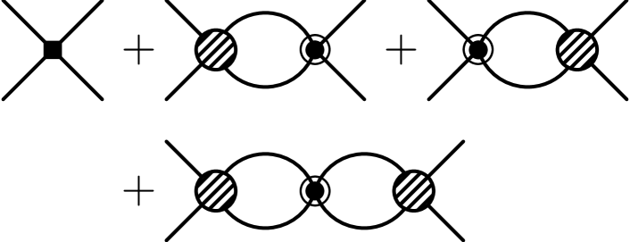
Figure 4: NLO correction to the $N\!N$ scattering amplitude from the $C_{2}$ interaction (circled circle).

This procedure can be generalized to higher orders and other operators. At N²LO we must consider two insertions of $C_{2}$ and one insertion of $C_{4}$; the latter is determined entirely in terms of $r_{0}^{2}$, the shape parameter emerging at N³LO Kaplan et al. (1998a, b); van Kolck (1999b). Generally, enhancements depend on the partial waves involved. The interactions contributing to such waves are operators in the “$\cdots$” of Eq. (13) that make $T$ dependent on the scattering angle. There is no enhancement for operators that contribute only to higher waves, as long as there are no other low-energy poles as is the case in $N\!N$ scattering. Thus, for example, a $P$-wave operator leading to a term $\propto\mathbf{k}^{\prime}\cdot\mathbf{k}$ appears first at N³LO. The enhancement is only partial for operators that connect an $S$ wave to other waves. The short-range tensor force that connects $S$ and $D$ waves is present at N²LO because it is enhanced by one power of $M_{\text{lo}}^{-1}$ Chen et al. (1999a). The lowest orders in the potential are shown schematically in Fig. 5.

Figure 5: Diagrams representing the $AN$ nuclear potential in Pionless EFT. The order of the contributions is indicated as $\mathcal{O}(Q^{\mu}/M_{\text{hi}}^{\mu})$, $\mu\geq 0$, where $Q\sim M_{\text{lo}}$ and $M_{\text{hi}}\sim m_{\pi}$, so that circles around the central solid circle denotes inverse powers of $M_{\text{hi}}$.

Summarizing, the $2N$ potential (16) is a particularly simple form of Eq. (9) where there are no non-analytic functions and

$$\mu=d/2\;\;(s_{2}=2)\ \ \text{,}\ \ \mu=d+1-s_{2}\;\;(s_{2}=0,1)\,,$$ (19)

$$\tilde{\mathcal{N}}=\mathcal{O}\left((4\pi)^{A-1}m_{N}^{-1}M_{\text{lo}}^{5-3A}\right)\,,$$ (20)

with $A=2$, $d$ the number of derivatives, and $s_{2}=0,1,2$ the number of $S$ waves connected by the operator Bedaque and van Kolck (1998); van Kolck (1997); Kaplan et al. (1998a, b); Bedaque et al. (1998); van Kolck (1999b). Using the standard graph equalities to eliminate the number of internal lines $I$ and loops $L$, $I=\sum_{i}V_{i}+L-1$ and $I=-A+\sum_{i}f_{i}V_{i}/2$, where $V_{i}$ is the number of vertices with $f_{i}$ nucleon lines, we obtain Eq. (5) for the amplitude with

$$\nu=\sum_{i}V_{i}\mu_{i}\ \ \text{,}\ \ \mathcal{N}=\mathcal{O}\left((4\pi)^{A-1}m_{N}^{-1}M_{\text{lo}}^{5-3A}\right)\,.$$ (21)

Assuming $M_{\text{lo}}\sim\gamma_{d}$, a rough estimate of the expansion parameter is $M_{\text{lo}}/M_{\text{hi}}\sim\gamma_{d}/m_{\pi}\sim 1/3$.

II.2.3 Regularization and renormalization

Loops in a quantum field theory are often not convergent, and the same in true in Pionless EFT. Observables are rendered finite by renormalization. For example, if we introduce a regulator function $f(x)$, the nucleon bubble integral becomes

$$I_{0}(k)=m_{N}\int\!\!\frac{\mathrm{d}^{3}q}{(2\pi)^{3}}\frac{f(\mathbf{q}^{2}/\Lambda^{2})}{k^{2}-\mathbf{q}^{2}+\mathrm{i}\varepsilon}\\ ={-}\frac{m_{N}}{4\pi}\left[\theta_{1}\Lambda-\sqrt{-k^{2}-\mathrm{i}\varepsilon}+\mathcal{O}(k^{2}/\Lambda)\right]\,,$$ (22)

where $\theta_{1}$ is a dimensionless number that depends on the form of $f(x)$ (for example, $\theta_{1}=2/\pi$ for a step function). With Eq. (II.2.1) truncated at the scattering length as a renormalization condition, the choice

$$C_{0}(\Lambda)=\frac{4\pi}{m_{N}}\frac{1}{1/a_{0}-\theta_{1}\Lambda}$$ (23)

ensures, to this order, that the physical amplitude is independent of $\Lambda$, up to corrections that vanish as $\Lambda\to\infty$. The latter can be removed by higher-order LECs, such as $C_{2}(\Lambda)$. It is the non-analytic dependence on energy, which is regulator independent, that characterizes a loop. The corresponding term in Eq. (22) is an explicit example of the estimates (15) and (15).

Schemes and power counting

In early stages, there was much confusion about whether or not the choice of regularization should be understood to affect the power-counting scheme. The difference between the artificial regulator parameter $\Lambda$ and the breakdown scale $M_{\text{hi}}$ of the theory has not always been appreciated. For example, Kaplan et al. (1998a) have argued that $C_{0}\propto\Lambda^{-1}$ would again give a theory with a very limited range of applicability. The need to choose $\Lambda\stackrel{{\scriptstyle>}}{{{}_{\sim}}}M_{\text{hi}}$ in order to suppress regulator artifacts $\sim\mathcal{O}(1/\Lambda)$ does seem to invalidate the scaling $C_{0}\propto M_{\text{lo}}^{-1}$, but there are correlations among the diagrams which are captured by determining $C_{0}(\Lambda)$ after resummation, reflecting the original $M_{\text{lo}}$ counting.

If one uses dimensional regularization to render integrals finite, the $I_{0}$ bubble does not have a pole in four spacetime dimensions, so in the minimal subtraction scheme there would be no divergence at all. Instead of this, Kaplan et al. (1998a) advocate explicitly subtracting the pole in three dimensions (corresponding to the linear divergence in the cutoff scheme), thereby introducing a renormalization scale $\mu$, which can be chosen freely, and giving Eq. (23) with $\theta_{1}\Lambda\to\mu$. This procedure, called “power divergence subtraction” (PDS), makes the need for resummation of the bubble diagrams more transparent. Picking $\mu\sim Q$, the running coupling $C_{0}$ scales like $Q^{-1}$, implying again that each diagram in Fig. 3 is of the same order. With this scheme, power counting is “manifest” in the sense that it is reflected by the scaling of coupling constants even after renormalization has been carried out. Phillips et al. (1999) have shown that if all poles of a divergent loop integral are subtracted—like the original PDS, one particular choice of infinitely many possibly schemes—one recovers exactly the same result as with a simple momentum cutoff.

Under an appropriate power counting, changing the low-energy points used as renormalization conditions affects the running of the LECs by $1/\Lambda$ terms, and leads to the same $T$ matrix up to higher-order terms. Taking for example the pole position $\mathrm{i}\gamma$ instead of zero energy generates the LO amplitude with $1/a_{0}\to\gamma$; the relative difference is an NLO correction $\sim r_{0}/a_{0}=\mathcal{O}(M_{\text{lo}}/M_{\text{hi}})$. While the a priori EFT error estimate is always determined by neglected higher orders, the freedom to choose what input parameters are used at a given order can improve agreement of the central values with experimental data. Gegelia (1999a) discusses the relation of subtractive renormalization to the other approaches mentioned above.

It was eventually realized Lepage (1997) that cutoff variation can be used (and is particularly useful in numerical calculations) as a diagnostic for missing interactions at a given order, an example of which will be given in Sec. II.3.2. Long and Yang (2012b) pointed out that also the leading residual cutoff dependence can be used to infer the existence of next-order operators. Equation (22), for example, indicates that $C_{2}\propto M_{\text{hi}}^{-1}$ in order for the residual dependence on $\Lambda\stackrel{{\scriptstyle>}}{{{}_{\sim}}}M_{\text{hi}}$ to be no larger than NLO. Thus renormalization provides guidance for the power counting.

Subleading resummation

Experience with nonsingular potentials makes it almost automatic to solve the Schrödinger equation exactly with a truncation of the potential (16). At LO this is equivalent to the resummation (14). Renormalization of the truncation at the level of $C_{2}$, however, leads to $r_{0}\stackrel{{\scriptstyle<}}{{{}_{\sim}}}\Lambda^{-1}$ Cohen (1997); Phillips and Cohen (1997); Scaldeferri et al. (1997), a version of the so-called “Wigner bound” Wigner (1955). This is problematic for $N\!N$ scattering where $r_{0}>0$. At first interpreted as a failure of EFT, this observation reveals instead the danger of resumming subleading singular potentials van Kolck (1999b). Such a resummation includes a subset of arbitrarily high-order contributions without all the LECs needed for perturbative renormalization, such as $C_{4}$ when $C_{2}$ is inserted twice at N²LO. It is still possible to work with a fixed cutoff that reproduces $r_{0}$, at the cost of losing the ability to use cutoff variation $\Lambda\stackrel{{\scriptstyle>}}{{{}_{\sim}}}M_{\text{hi}}$ as a diagnostic for missing interactions. Moreover, there is no guarantee that results for other observables will be any better than those obtained from a perturbative treatment of subleading corrections. An example is given by Stetcu et al. (2010a).

II.2.4 Renormalization group

Running coupling

Imposing renormalizability of physical amplitudes leads to solutions of RG equations. Their detailed form depends on the regularization scheme. For example, in PDS one finds for the dimensionless coupling constant $\hat{C_{0}}\equiv m_{N}\mu C_{0}/(4\pi)$ Kaplan et al. (1998a),

$$\mu\frac{\mathrm{d}}{\mathrm{d}\mu}\hat{C_{0}}=\hat{C_{0}}(1+\hat{C_{0}})\,,$$ (24)

where the right-hand side is given by the beta function. It is convenient to consider the flow of $\hat{C_{0}}$ instead of $C_{0}$ in order to separate the behavior of the operator from the behavior of the coupling constant. The RG equation (24) has two fixed points: the free fixed point $\hat{C_{0}}=0$ and a nontrivial fixed point $\hat{C_{0}}=-1$ Weinberg (1991), which correspond to $a_{0}=0$ and to the unitary limit $1/a_{0}=0$, respectively. Similar equations can be derived for all coupling constants in the effective Lagrangian, and the beta function will in general change as one goes to higher orders. Thus the expansion in Pionless EFT can be thought of as an expansion around the unitary limit of infinite scattering length, similar to the expansion in Chiral EFT around the chiral limit of vanishing quark masses. An equation similar to (24) holds for a simple momentum cutoff $\Lambda$, leading then to Eq. (23). In dimensional regularization with minimal subtraction, on the other hand, the coupling $C_{0}$ is independent of $\mu$ Kaplan et al. (1996). In this scheme the unitary limit cannot be reached for any finite value of the coupling.

Wilsonian renormalization group

The RG is more generally useful to study the behavior of the EFT. Extending previous work Weinberg (1990, 1991); Adhikari and Frederico (1995); Adhikari and Ghosh (1997); Beane et al. (1998b); Phillips et al. (1998); Kaplan et al. (1998a, b, 1999b), Birse et al. (1999) studied the RG flow of an effective potential of the form

$$V_{2N}(\mathbf{p}^{\prime},\mathbf{p},k)=V_{2N}(\mathbf{p}^{\prime},\mathbf{p})+C_{02}k^{2}+\cdots\,,$$ (25)

where the additional energy-dependent terms compared to Eq. (16) come from a different choice of operators in the effective Lagrangian (13). It is possible to trade energy dependence for momentum dependence and vice versa by field redefinitions or, alternatively, using the equation of motion. Within a Wilsonian formulation of the RG Wilson (1983), demanding that the off-shell amplitude stays invariant under a decrease in the momentum cutoff $\Lambda$ in the Lippmann-Schwinger equation defines a “running” potential $V(p,p^{\prime},k,\Lambda)$ which satisfies

$$\frac{\partial V}{\partial\Lambda}=\frac{m_{N}}{2\pi^{2}}V(p^{\prime},\Lambda,k,\Lambda)\frac{\Lambda^{2}}{\Lambda^{2}-k^{2}}V(\Lambda,p,k,\Lambda)\,.$$ (26)

Defining further a rescaled potential $\hat{V}$ by multiplying all quantities with appropriate powers of $\Lambda$, Birse et al. (1999) showed that in the limit where $\Lambda\to 0$ there exist two IR fixed points satisfying $\partial\hat{V}/\partial\Lambda=0$. One of these, $\hat{V}=0$, is trivial whereas the second, nontrivial one corresponds to the unitary limit. Additional fixed points are accessible with further fine tuning Birse et al. (2016). An extensive study including also higher waves was carried by Harada and Kubo (2006) and Harada et al. (2009). The RG analysis captures the results obtained from Feynman diagrams, which yield directly the solutions of the RG equations. It unifies both the natural and fine-tuned cases discussed in Sec. II.2.2, and it is possible to derive the power counting for either case by studying perturbations of the potential around the fixed points.

II.2.5 Dibaryon fields

It is possible to efficiently capture the physics associated with the shallow $S$-wave two-body states by introducing in the effective Lagrangian “dimeron” (“molecular” or, here, “dibaryon”) fields with their quantum numbers, an idea first introduced in EFT by Kaplan (1997). For any single channel we can write, instead of (13),

$${\!\mathcal{L}=\psi^{\dagger}\Big{(}\mathrm{i}\partial_{0}+\frac{\boldsymbol{\nabla}^{2}}{2m_{N}}\Big{)}\psi+g\left[d^{\dagger}(\psi\psi)+\mathrm{H.c.}\right]}\\ {\hbox{}+d^{\dagger}\Big{[}\eta\Big{(}\mathrm{i}\partial_{0}+\frac{\boldsymbol{\nabla}^{2}}{4m_{N}}\Big{)}-\Delta\Big{]}d+\cdots\,,}$$ (27)

where $\eta=\pm 1$ is a parameter that determines the sign of the effective range. It will be fixed to $\eta=-1$ in the remainder of this section to ensure $r_{0}>0$. Instead of $C_{0}$ and $C_{2}$, we have the new parameters $\Delta$ (the “residual mass”) and $g$. With this choice, nucleons no longer couple directly, but only through the $s$-channel exchange of the dibaryon $d$. If one neglects the kinetic term for this field, it is possible to recover the leading terms in Eq. (13) by using the equation of motion for $d$,

$${d=\frac{g}{\Delta}\psi\psi\,,}$$ (28)

and identifying $C_{0}=-g^{2}/\Delta$. Because of this redundancy, without loss of generality one may fix $g$ at LO; a convenient choice is $g^{2}\equiv 4\pi/m_{N}$ Grießhammer (2004) so that $\Delta=-1/a_{0}$ represents the low-energy scale $M_{\text{lo}}$. The $d$ kinetic term leads to both energy- and momentum-dependent four-nucleon-field interactions, corresponding to a choice of operators that differs from Eq. (13), but can be shown to be equivalent up to higher orders and field redefinitions Bedaque and Grießhammer (2000).

The original bubble series with $C_{0}$ vertices turns into a self-energy correction for the dibaryon field: whereas the tree-level bare propagator is just $\mathrm{i}D(p_{0},\mathbf{p})={-}\mathrm{i}/\Delta$, summing up all bubble insertions as shown in Fig. 6 gives the full LO propagator as

$$\mathrm{i}D^{(0)}(p_{0},\mathbf{p})={-}\mathrm{i}\left[\Delta+g^{2}\,I_{0}\!\left(\sqrt{m_{N}p_{0}-\mathbf{p}^{2}/4}\right)\right]^{-1}\,.$$ (29)

The center-of-mass $N\!N$ scattering amplitude is recovered by attaching nucleon-dibaryon vertices on both ends: $T^{(0)}={-}g^{2}D^{(0)}(p_{0}=k^{2}/m_{N},\mathbf{p}=0)$.

Figure 6: Bubble sum for the dressed dibaryon propagator obtained from the bare propagator (double dashed line).

Not only is the dibaryon formalism useful to study processes with deuterons in the initial and/or final state (see below), where it can conveniently be used as an interpolating field, but it also makes higher-order corrections particularly simple. For example, where before we had to insert $C_{2}$ vertices in different places (see Fig. 4), we now only have to insert the dibaryon kinetic-energy operator into the LO propagator, giving

$$\mathrm{i}D^{(1)}(p_{0},\mathbf{p})=\mathrm{i}\left(p_{0}-\frac{\mathbf{p}^{2}}{4m_{N}}\right)\left(D^{(0)}(p_{0},\mathbf{p})\right)^{2}$$ (30)

at NLO. As in the case without dibaryons, renormalization is carried out by relating $D^{(1)}$ to the NLO amplitude correction $T^{(1)}(k)$ and matching to the effective-range term in Eq. (II.2.1). A difference is, however, that this is now carried out with an energy-dependent operator—note the dependence of Eq. (30) on the Galilei-invariant energy $\tilde{p}_{0}=p_{0}-\mathbf{p}^{2}/(4m_{N})$—whereas our choice of $C_{2}$ terms in Eq. (13) only includes momentum-dependent operators. The NLO component of $g$ can be adjusted to reproduce $r_{0}$, and $g$ and $\Delta$ are now independent. This means that these parameters have RG runnings that differ from those for $C_{0}$ and $C_{2}$ Birse et al. (1999).

With a dibaryon, range effects can be resummed using the propagator

$$\mathrm{i}D^{\text{resum}}(p_{0},\mathbf{p})=\frac{{-}\mathrm{i}}{\Delta+g^{2}\,I_{0}\!\left(\sqrt{m_{N}\tilde{p}_{0}\vphantom{2^{3}}}\right)-\tilde{p}_{0}}\,.$$ (31)

The Wigner bound is automatically avoided by allowing the dibaryon to be a ghost field. In fact, Beane and Savage (2001) proposed that the relatively large sizes of the $N\!N$ effective ranges (about $2m_{\pi}^{-1}$) justify their resummation as an LO effect. However, this procedure leads to two $S$-matrix poles per channel and is thus more likely to be interpreted as a resummation of NLO interactions, which includes additional higher-order effects.

II.2.6 Spin-isospin projection and parametrizations

For a fixed $N\!N$ channel it is convenient to use the effective Lagrangian (13), with $\psi$ a nucleon field for which the combination $\psi^{\dagger}\psi$ has definite spin and isospin $(S,I)$. The Pauli principle dictates that only isospin-triplet $\mathrm{t}\equiv(0,1)$ and isospin-singlet $\textrm{s}\equiv(1,0)$ are allowed combinations. We use subscripts “$\mathrm{s}$” and “$\mathrm{t}$” here in reference to isospin, with a warning that the same subscripts are sometimes used in reference to spin. To go beyond the description of an isolated two-nucleon system, it is desirable to treat both combinations on the same footing. To this end, it is convenient to introduce a nucleon field $N$ that is a doublet in both spin and isospin space, along with projection operators

$$(P_{\textrm{s}})^{i}=\sigma^{2}\sigma^{i}\tau^{2}/\sqrt{8}\ \ \text{,}\ \ (P_{\textrm{t}})^{A}=\sigma^{2}\tau^{2}\tau^{A}/\sqrt{8}\,,$$ (32)

where $\sigma^{i}$ ($\tau^{A}$) denotes the three Pauli matrices in spin (isospin) space, and we have used lower- (upper-) case indices to further distinguish the two spaces. The Lagrangian for the $N\!N$ system can then be written as

$$\mathcal{L}=N^{\dagger}\left(\mathrm{i}\partial_{0}+\frac{\boldsymbol{\nabla}^{2}}{2m_{N}}\right)N-\frac{C_{0\textrm{s}}}{2}(N^{T}P_{\textrm{s}}N)^{\dagger}(N^{T}P_{\textrm{s}}N)\\ -\frac{C_{0\textrm{t}}}{2}(N^{T}P_{\textrm{t}}N)^{\dagger}(N^{T}P_{\textrm{t}}N)+\cdots\,,$$ (33)

where the ellipses represent analogous terms with $C_{2\textrm{s/t}}$ as well as higher-order operators. Fierz rearrangements can be used to generate equivalent interactions. Analogously, Eq. (27) is generalized to the nuclear case by introducing two dibaryon fields—one for each $N\!N$ $S$-wave channel— using the same projection operators $P_{\textrm{s},\textrm{t}}$ Bedaque and van Kolck (1998).

The two channels are somewhat different concerning both sign and magnitude of the scattering lengths. However, it has been customary to treat both $a_{\mathrm{s}}^{-1}$ and $|a_{\mathrm{t}}|^{-1}$ as $M_{\text{lo}}$, although we return to this issue in Sec. II.2.7. The ERE, Eq. (II.2.1), has a certain radius of convergence, set by the nearest singularity to the expansion point $k^{2}=0$. The pion-exchange cut on the imaginary $k$ axis starting at $m_{\pi}$/2 leaves the deuteron pole within the radius of convergence of the ERE, and indeed it is well known that the properties of this pole can be expressed in terms of the ERE parameters Goldberger and Watson (1967), cf. Sec. II.2.1. For example, the deuteron binding momentum is

$$\gamma_{d}=\frac{1}{a_{\rm s}}\left(1+\frac{r_{\rm s}}{2a_{\mathrm{s}}}+\cdots\right)\,.$$ (34)

Alternatively, and this is in fact what was done first historically Bethe (1949), one can perform the ERE directly about this pole (i.e., about the point $\mathrm{i}\gamma_{d}$ in the complex momentum plane),

$$k\cot\delta_{d}(k)={-}\gamma_{d}+\dfrac{\rho_{d}}{2}\big{(}k^{2}+\gamma_{d}^{2}\big{)}+\cdots\,,$$ (35)

where $\rho_{d}\simeq 1.765\leavevmode\nobreak\ \mathrm{fm}$ de Swart et al. (1995) is the deuteron effective range. The motivation for using Eq. (35) instead of the ERE about zero momentum is that it captures the exact location of the pole already at LO. Grießhammer (2004) extended the procedure to the ${}^{1}S_{0}$ channel, where it is possible to define the ERE about the virtual-state pole.

The first detailed comparison of the ${}^{3}S_{1}$ phase shift obtained in Pionless EFT with empirical values was carried out up to N²LO by Chen et al. (1999a), with LECs fitted to Eq. (35). In Fig. 7 we show results fitted to Eq. (II.2.1) instead, which are qualitatively similar: convergence is seen at low energies and already at NLO a very good description is achieved. The corresponding results for ${}^{1}S_{0}$ up to N²LO were presented by Beane et al. (2001b).

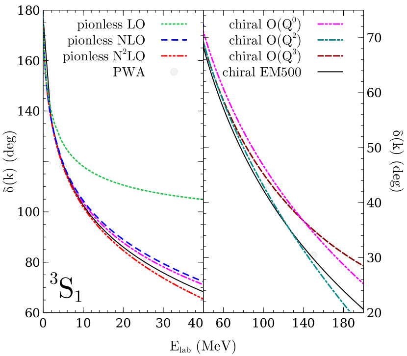
Figure 7: The $N\!N$ scattering phase shift $\delta$ as a function of the nucleon laboratory energy $E_{\text{lab}}$ in the ${}^{3}S_{1}$ partial wave for Pionless EFT and Chiral EFT at various orders Long and Yang (2012a) (results kindly provided by C.-J. Yang), and the chiral potential “EM500” Entem and Machleidt (2003). For comparison we show the partial-wave analysis (PWA) of Navarro Pérez et al. (2013), with error bars smaller than the symbols.

II.2.7 Coulomb effects and other isospin breaking

Since almost all nuclear systems involve more than one proton, the inclusion of electromagnetic effects is generally important. In the low-energy regime, the dominant effect is given by “Coulomb photons”, i.e., the familiar, static potential ($\sim\alpha/r$) between charged particles. It originates from the replacement of derivatives in the effective Lagrangian with covariant ones,

$$D_{\mu}=\partial_{\mu}+\mathrm{i}eA_{\mu}\hat{Q}\,,$$ (36)

where $\hat{Q}$ is an appropriate charge operator (e.g., $\hat{Q}=(1+\tau_{3})/2$ for nucleons). The Coulomb photon-nucleon coupling $\mathrm{i}e$ comes from the gauging of the nucleon time derivative in Eq. (33), while the Coulomb-photon “propagator” is $\mathrm{i}/(\mathbf{q}^{2}+\lambda^{2})$, where $\lambda$ is an IR-regulating photon mass that is eventually taken to zero. Finer electromagnetic effects enter through operators with more covariant derivatives and also directly through the field strength, or alternatively the electric ($E_{i}=\partial_{0}A_{i}-\partial_{i}A_{0}$) and magnetic ($B_{i}=\epsilon_{ijm}\partial^{j}A^{m}$) fields.

Kong and Ravndal (1999b, 2000) were the first to study proton-proton ($pp$) scattering in Pionless EFT. The challenge here lies in the fact that the Coulomb interaction is important at very low energies: we see from Eq. (10) for the Coulomb potential $V\sim e^{2}/Q^{2}$ that Coulomb is nonperturbative for ${Q\stackrel{{\scriptstyle<}}{{{}_{\sim}}}\alpha m_{N}/2\equiv k_{C}}$, which is in the low-energy region of Pionless EFT. Subtracting the pure-Coulomb amplitude $T_{C}$ from the full amplitude $T$, one can write

$$T_{SC}=T-T_{C}={-}\frac{4\pi}{m_{N}}\frac{\mathrm{e}^{2\mathrm{i}\sigma_{C}}}{k\cot\delta_{pp}(k)-\mathrm{i}k}$$ (37)

in terms of the “subtracted” $pp$ phase shift $\delta_{pp}(k)$ and the pure-Coulomb phase shift $\sigma_{C}=\arg{\Gamma(1+\mathrm{i}\eta)}$. Renormalization can be carried out by matching to the “Coulomb-modified” ERE Bethe (1949),

$$C_{\eta}^{2}\left(k\cot\delta_{pp}(k)-\mathrm{i}k\right)+\alpha m_{N}H(\eta)\\ ={-}\frac{1}{a_{pp}}+\frac{r_{pp}}{2}k^{2}+\cdots\,,$$ (38)

where $a_{pp}\simeq-7.8$ fm and $r_{pp}\simeq 2.8\leavevmode\nobreak\ \mathrm{fm}$ Bergervoet et al. (1988) are the ERE parameters, $C_{\eta}^{2}=2\pi\eta[\exp(2\pi\eta)-1]^{-1}$ is the Sommerfeld factor in terms of $\eta=k_{C}/k$, and $H(\eta)=\Re[\psi(1+\mathrm{i}\eta)]-\ln\eta+\mathrm{i}C_{\eta}^{2}/(2\eta)$ in terms of the digamma function $\psi$. It should be emphasized that the $pp$ scattering amplitude, and thus also the effective range parameters, are always defined in the presence of the Coulomb interaction and cannot be divided into strong and electromagnetic parts in a model-independent way Kong and Ravndal (1999b); Gegelia (2004). For particles with non-unit charges the definition of the Coulomb momentum $k_{C}$ is generalized in Sec. III, see Eq. (68).

In Pionless EFT, $T_{SC}$ is obtained by replacing all empty bubbles in Fig. 3 with the dressed one shown in Fig. 8. The initial and final-state Coulomb interactions are accounted for by the construction in Eq. (37). “Dressing” here refers to resumming the Coulomb interaction to all orders between each pair of $C_{0}$ vertices, which Kong and Ravndal (1999b, 2000) were able to do using a known analytic expression for the pure Coulomb Green’s function. With dimensional regularization,

$$\frac{4\pi}{m_{N}C_{0}^{pp}(\mu)}=\frac{1}{a_{{pp}}}-\mu+\alpha m_{N}\left(\frac{1}{\varepsilon}+\ln\frac{\mu}{\alpha m_{N}}+\text{const.}\right).$$ (39)

The term linear in the renormalization scale $\mu$ comes from the PDS prescription, but Coulomb exchange now introduces an additional logarithmic divergence, reflected in the pole in $\varepsilon=d-3$, where $d$ is the number of spatial dimensions. Range corrections have been considered at NLO by Kong and Ravndal (2000) and at N²LO by Ando et al. (2007). An equivalent formulation in terms of a $pp$ dibaryon exists Ando and Birse (2010). The RG analysis of Birse et al. (1999) discussed in Sec. II.2.4 has also been extended to the charged-particle sector Barford and Birse (2003); Ando and Birse (2008).

Figure 8: Bubble diagram dressed with Coulomb exchange (wavy line).

The LEC $C_{0}^{pp}=C_{0\textrm{t}}+\Delta C_{0(+)}$ in Eq. (39) contains an isospin-dependent contribution $\Delta C_{0(+)}$, which is a short-range (or “indirect”) electromagnetic effect. The EFT includes also isospin breaking from the quark masses van Kolck (1993, 1995). While electromagnetic interactions break isospin more generally (“charge dependence”), effects linear in the quark masses break charge symmetry (a rotation of $\pi$ around the second axis in isospin space) specifically. Introducing the projectors $P_{(\pm)}=(P_{\mathrm{t}}^{1}\mp\mathrm{i}P_{\mathrm{t}}^{2})/\sqrt{2}$ onto the $pp$/$nn$ channel, the isospin-breaking Lagrangian takes the form

$$\mathcal{L}_{\textrm{ib}}=\delta m_{N}N^{\dagger}\tau_{3}N-\frac{\Delta C_{0(+)}}{2}(N^{T}P_{(+)}N)^{\dagger}(N^{T}P_{(+)}N)\\ -\frac{\Delta C_{0(-)}}{2}(N^{T}P_{(-)}N)^{\dagger}(N^{T}P_{(-)}N)+\cdots\,.$$ (40)

NDA (11) indicates that the neutron-proton mass splitting $\delta m_{N}=\mathcal{O}(\varepsilon{\bar{m}},\alpha m_{N}/(4\pi))$. It is well known that the two types of contributions are comparable in magnitude, $\varepsilon{\bar{m}}\sim\alpha m_{N}/4\pi$, valid up to a (scale-dependent) factor of a few, but have opposite signs, the quark masses tilting the balance in favor of the neutron. The mass-splitting term can be removed by a redefinition of the nucleon field Friar et al. (2004), and reappears as an $\mathcal{O}(\delta m_{N}/m_{N})$ effect in the nucleon kinetic term. The most important quark-mass effects in the $N\!N$ system lie in the short-range LECs $\Delta C_{0(\pm)}$. The reduced quark mass is $(\varepsilon{\bar{m}})_{\mathrm{red}}=\varepsilon{\bar{m}}/M_{\text{hi}}$ and, together with the $S$-to-$S$-wave enhancement discussed in Sec. II.2.2, leads to $(a_{nn}-a_{\mathrm{t}})/a_{\mathrm{t}}\sim\Delta C_{0(-)}/C_{0\mathrm{t}}=\mathcal{O}(\varepsilon{\bar{m}}\,a_{\mathrm{t}})\simeq 0.2$, cf. König et al. (2016). A similar contribution exists for $\Delta C_{0(+)}$ which is, however, dominated by the electromagnetic contribution $\Delta C_{0(+)}/C_{0\textrm{t}}=\mathcal{O}(\alpha m_{N}a_{\mathrm{t}})$, consistent with Eq. (39).

For most of the region of validity of Pionless EFT, $Q\stackrel{{\scriptstyle>}}{{{}_{\sim}}}\alpha m_{N}$ and all electromagnetic interactions are expected to be perturbative. In this region, $Q\stackrel{{\scriptstyle>}}{{{}_{\sim}}}1/a_{\mathrm{t}}$ as well. König et al. (2016) developed an expansion in powers of $\alpha m_{N}/Q$ and $1/(Qa_{\mathrm{t}})$ in addition to the standard $Q/M_{\text{hi}}$ expansion. For simplicity, they paired the expansions by taking $\alpha m_{N}\sim a_{\mathrm{t}}^{-1}=\mathcal{O}(M_{\text{lo}}^{2}/M_{\text{hi}})$ and $\varepsilon{\bar{m}}=\mathcal{O}(M_{\text{lo}}^{3}/M_{\text{hi}}^{2})$. In this case, LO in the ${}^{1}S_{0}$ channel consists of the isospin-symmetric unitary amplitude, that is, Eq. (II.2.1) with $k\cot\delta_{\textrm{t}}=0$. The first short-range and electromagnetic corrections break isospin symmetry at NLO, reproducing $a_{pp}$ and leading to equal scattering lengths in the other two ${}^{1}S_{0}$ isospin channels. In addition, at NLO there is the standard, isospin-symmetric $C_{2\mathrm{t}}$ interaction, while quark-mass effects (and the $nn$ splitting from $np$) first enter at N²LO. This is consistent with the observed relation $r_{pp}\simeq r_{\mathrm{t}}$.

II.2.8 External currents

One of the great advantages of the EFT approach is that it is straightforward to include external currents in addition to interactions between nucleons. Power counting leads to a systematic expansion of current operators, which had previously been classified only as one-body and many-body pieces (also known as “meson-exchange currents”).

Photons are introduced in the effective Lagrangian as described above. In addition, weak interactions are accounted for by current-current interactions, where the currents have the well-known vector-axial ($V-A$) form. Power counting is similar to that described in Sec. II.2.2, with current operators subject to the same enhancement by powers of $M_{\text{lo}}^{-1}$ when $S$ waves are involved Chen et al. (1999a). Electromagnetic couplings were analyzed with the Wilsonian RG by Kvinikhidze and Birse (2018).

The earliest example in the context of Pionless EFT are calculations of static deuteron properties by Chen et al. (1999a), paralleling previous work by Kaplan et al. (1999b) and Savage et al. (1999) in Chiral EFT with perturbative pions. Chen et al. (1999a) calculated several deuteron properties (charge, magnetic dipole and electric quadrupole form factors, as well as electric polarizabilities) beyond LO, including also relativistic corrections. Results were found to be in very good agreement with both experimental data and, at low orders, with those obtained from effective-range theory Lucas and Rustgi (1968); Friar and Fallieros (1984); Wong (1994). At higher orders, the EFT goes beyond the effective-range approach (which is based on input from elastic $N\!N$ scattering only) because new operators appear with undetermined coefficients. For example, there are magnetic four-nucleon-one-photon couplings at NLO,

$$\mathcal{L}_{\text{mag}}^{(1)}=eL_{1}\left(N^{T}P^{i}_{\textrm{s}}N\right)^{\dagger}\left(N^{T}P^{3}_{\textrm{t}}N\right)B_{i}\\ -\mathrm{i}eL_{2}\,\epsilon_{ijk}\left(N^{T}P^{i}_{\textrm{s}}N\right)^{\dagger}\left(N^{T}P^{j}_{\textrm{s}}N\right)B^{k}+\mathrm{H.c.}\,.$$ (41)

This is the two-nucleon analog of the single-particle “Pauli term” that describes the direct $\vec{S}\cdot\vec{B}$ coupling of the nucleon spin to a magnetic field, which accounts for the nucleon anomalous magnetic moment. Here $L_{1}$ and $L_{2}$ are LECs that contribute to the deuteron dipole magnetic moment as well as to the capture process $np\to d\gamma$.

Motivated by the original work of Bethe (1949) and Bethe and Longmire (1950), Phillips et al. (2000) proposed a new scheme to incorporate NLO and higher orders in processes involving the deuteron. Up to higher-order corrections contained in the ellipses we can read off the residue of the deuteron pole from Eq. (35),

$$Z_{d}=\left(1-\gamma_{d}\rho_{d}\right)^{-1}=1+\gamma_{d}\rho_{d}+(\gamma_{d}\rho_{d})^{2}+\cdots\,.$$ (42)

This residue is directly related to the long-range tail of the deuteron wavefunction in configuration space. Phillips et al. (2000) argued that convergence of deuteron observables (at least those sensitive to the long-range tail of the wavefunction) can be dramatically improved by fitting to $Z_{d}$ exactly right at NLO—rather than building it up perturbatively as given in Eq. (42)—while not spoiling convergence for the ${}^{3}S_{1}$ phase shifts.

A deuteron dibaryon field (see Sec. II.2.5) is particularly convenient for processes with external deuterons. The dressed dibaryon can be used directly as an interpolating field to define the $S$ matrix, provided its wavefunction renormalization is properly taken into account. With a dibaryon, the effects of a resummation of the effective range can be assessed Beane and Savage (2001); Ando and Hyun (2005).

A number of processes has been carefully addressed with these tools. A precise and controlled theoretical prediction of the $np\to d\gamma$ cross section is important because it enters as an input parameter into big-bang nucleosynthesis calculations. The low-energy values required are difficult to access experimentally, but are ideally suited for an application of Pionless EFT. The pionless analysis of this process started by Chen et al. (1999a) was refined in subsequent papers Chen et al. (1999b); Chen and Savage (1999). Rupak (2000) carried out the analysis to N⁴LO, giving a prediction that is accurate to a theoretical uncertainty below 1%. This reaction was revisited with dibaryon fields at NLO and a resummation of effective-range effects by Ando et al. (2006).

The related processes of deuteron electro- and photodisintegration are experimentally accessible, and discrepancies between phenomenological potential models and data have been reported. Dibaryon fields implementing a resummation of range effects have been used to N²LO for $ed\to e^{\prime}pn$ Christlmeier and Grießhammer (2008) and $d\gamma\to np$ Ando et al. (2011); Song et al. (2017a), with results generally supporting phenomenological models. For example, Christlmeier and Grießhammer (2008) concluded that no consistent theoretical calculation could describe the data because the EFT calculation, unlike the potential-model approach, comes with a rigorous uncertainty estimate. Subsequently, the resolution of a problem with the data analysis gave agreement between experiment and the EFT calculation Ryezayeva et al. (2008), see Fig. 9.

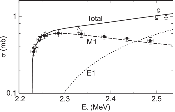
Figure 9: Total cross section $\sigma$ for deuteron electrodisintegration as function of the photon energy $E_{\gamma}$. Good agreement is seen between measured data points and theoretical calculation (lines), which was achieved after the pionless calculation of Christlmeier and Grießhammer (2008) helped resolve a problem with the experimental analysis. Figure adapted from Ryezayeva et al. (2008) by H. W. Grießhammer. Courtesy of H. W. Grießhammer.

The proton-proton fusion process $pp\to de^{+}\nu_{e}$ is of similar importance for an understanding of the Sun. Obviously, Coulomb effects play an important role for this reaction at very low energies. Kong and Ravndal (1999a, c, 2001), building upon their previous work on $pp$ scattering (see Sec. II.2.7), presented a first calculation in Pionless EFT at NLO. This calculation was later extended to N⁴LO by Butler and Chen (2001). An NLO calculation using a dibaryon field to resum effective-range corrections was presented by Ando et al. (2008). Chen et al. (2013) extended the calculation of the astrophysical $pp$ S-factor to also include its energy derivatives.

The inverse process, neutrino-deuteron breakup scattering, was considered by Butler et al. (2001) to N²LO, along the lines of an earlier NLO perturbative-pion calculation Butler and Chen (2000). At NLO, the axial-vector counterparts of Eq. (41) appear, with two analogous LECs usually denoted $L_{1,A}$ and $L_{2,A}$. However, because of the quantum numbers of initial and final states, only the isovector $L_{1,A}$, which contributes to $pp\to de^{+}\nu_{e}$ as well, is significant. Various constraints on $L_{1,A}$ have been discussed by Butler et al. (2002), Chen et al. (2003), Balantekin and Yuksel (2003) and Chen et al. (2005a), confirming SNO’s conclusions about neutrino oscillations.

Additionally, single-nucleon properties can be inferred from nuclear data. Compton scattering is influenced by the nucleon polarizabilities, which are response functions that carry much information about hadron dynamics and thus QCD. While proton polarizabilities can be extracted directly, neutron polarizabilities can only be probed in nuclear Compton scattering. Compton scattering on the deuteron was studied to N²LO by Grießhammer and Rupak (2002), where effective ranges were resummed and $Z_{d}$ fitted. Values for the isoscalar, scalar electric and magnetic polarizabilities were extracted by Grießhammer and Rupak (2002). Additional features of the cross section were considered by Chen et al. (2005b) and Chen et al. (2005c). Sum rules for vector and tensor polarizabilities were given by Ji and Li (2004), while a low-energy theorem for the spin-dependent Compton amplitude was obtained by Chen et al. (2004a).

All in all, these calculations support the convergence of Pionless EFT for momenta below the pion mass, with the power counting discussed in Sec. II.2.2. They provide theoretically-controlled cross sections that impact astrophysics and particle physics. Heavier probes, such as pions Beane and Savage (2003a), can be considered as well through a heavy-field treatment. Most interesting for nuclear physics are processes with additional nucleons, which we consider next.

II.3 Light nuclei: bound and scattered

Pionless EFT extends effective-range theory into the nuclear realm, where it leads to a striking emergence of structure related to the Efimov phenomenon Efimov (1970a, 1981), which we discuss in more detail, in the context of Halo/Cluster EFT, in Sec. III.3.

II.3.1 Extension to three particles

The simplest three-body system that can be studied in Pionless EFT is neutron-deuteron ($nd$) scattering in the quartet $S$-wave channel (total spin $\nicefrac{{3}}{{2}}$ and zero orbital angular momentum). The Pauli principle dictates that only the same configuration can appear in the intermediate state. Bedaque and van Kolck (1998) calculated the $nd$ quartet scattering length in a framework using a deuteron dibaryon field (see Sec. II.2.5). The driving mechanism is the exchange of a nucleon (neutron) between in and outgoing deuterons. The EFT power counting gives that all diagrams with an arbitrary number of such exchanges are of the same order. Quite analogous to the two-body bubble chain they can be conveniently resummed into an integral equation for the scattering amplitude, shown diagrammatically in Fig. 10. The loop integrals are convergent, but for a numerical treatment it is still convenient to introduce a momentum cutoff. Resumming effective range corrections to all orders in the deuteron sector, Bedaque and van Kolck (1998) calculated the scattering length to be $6.33\leavevmode\nobreak\ \mathrm{fm}$, in very good agreement with the experimental value 6.35(2) $\mathrm{fm}$ Dilg et al. (1971). A perturbative treatment of effective-range corrections according to Eq. (35) gives $(5.09+0.98+0.21=6.28)\leavevmode\nobreak\ \mathrm{fm}$ to N²LO, with an estimated 3% uncertainty. The LO result of $5.09\leavevmode\nobreak\ \mathrm{fm}$ agrees with the much older result of Skorniakov and Ter Martirosian (1957) who used a zero-range model that is equivalent to Pionless EFT at LO. Bedaque et al. (1998) and Bedaque and Grießhammer (2000) extended the EFT calculation to $nd$ scattering at finite energy.

Figure 10: Integral equation for $nd$ scattering in the spin-quartet channel. A pair of similar, but coupled, equations describes the doublet channel.

II.3.2 The triton as a near-Efimov state

Three nucleons can also couple to an $S$-wave state with total spin $\nicefrac{{1}}{{2}}$, which is the channel of the trinucleon bound states: triton (³H) and helion (${}^{3}\mathrm{He}$). The formalism used to calculate quartet-channel scattering can be extended directly to the doublet channel, where now also ${}^{1}S_{0}$ intermediate states are allowed. The result can be written as an integral equation for the $nd$ $T$ matrix with the same structure as in Fig. 10, but for the two coupled channels $n+np$(${}^{3}S_{1}$) and $n+np$(${}^{1}S_{0}$) Skorniakov and Ter Martirosian (1957). The triton should show up as a pole in this amplitude at a negative energy $E={-}B({}^{3}\mathrm{H})={-}8.4818\leavevmode\nobreak\ \mathrm{MeV}$. Since its relevant momentum scale is given by $\gamma_{T}=\sqrt{2m_{N}B({}^{3}\mathrm{H})/3}\sim 80\leavevmode\nobreak\ \mathrm{MeV}$, it is within the expected range of validity of the EFT.

However, it has been known for a long time that the three-nucleon system is unstable when described solely with nonderivative two-body short-range interactions: as the range of such a potential is sent to zero, one encounters the “Thomas collapse,” i.e., the binding energy diverges Thomas (1935). Bedaque et al. (2000), generalizing their previous work on the three-boson system Bedaque et al. (1999a, b), showed that the same happens in Pionless EFT: as the cutoff $\Lambda\gg M_{\text{lo}}$ is increased, the ground-state energy grows as $\Lambda^{2}/m_{N}$, and excited states appear repeatedly. Since the $N\!N$ scattering lengths are large, one encounters an approximate realization of the Efimov effect Efimov (1970a, 1981), i.e., a tower of three-body states with the ratio of neighboring binding energies approaching a universal constant.

The three-body force

The scattering amplitude in the doublet channel, obtained from the integral equations analogous to Fig. 10, does not approach a stable limit as the cutoff is increased. This lack of renormalization is a genuine nonperturbative effect since every diagram generated by iterations is finite by itself. Bedaque et al. (2000) showed that the system can be stabilized by adding a nonderivative three-body contact interaction. Fierz rearrangements show that there is only one such interaction, which can be written in any one of various equivalents forms, for example

$$\mathcal{L}_{\text{3b}}={-}4h_{0}C_{0{\rm t}}^{2}\big{(}N^{T}(P_{\rm t})^{k}N\big{)}^{\dagger}\big{(}N^{\dagger}\sigma^{k}\sigma^{l}N\big{)}\big{(}N^{T}(P_{\rm t})^{l}N\big{)}\,,$$ (43)

where $h_{0}$ is a new LEC to be determined. In the formalism with dibaryon fields, every nucleon-exchange diagram has to be accompanied by a dibaryon-nucleon interaction with strength $h_{0}$, as shown in Fig. 11. Attaching the two-nucleon-dibaryon vertex $g$ from Eq. (27) on both dibaryon ends recovers the six-nucleon operator (43) in the theory without dibaryon field.

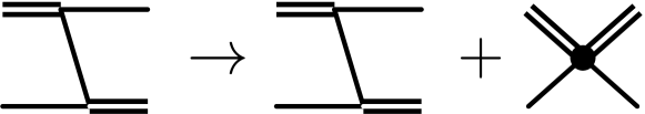
Figure 11: Modification of the driving mechanism in Fig. 10, with the LO three-body force (solid circled) in the $nd$ doublet channel.

The $3N$ force is symmetric Bedaque et al. (2000) under the group of combined spin and isospin transformations, Wigner’s $SU(4)$ Wigner (1937a, b). Because the two-body amplitude is also $SU(4)$ symmetric for momenta $a_{\mathrm{s}}^{-1}<Q<M_{\text{hi}}$ Mehen et al. (1999), the coupled integral equation illustrated in Fig. 10 is symmetric in the limit where all momenta are large compared to the inverse scattering lengths. This allowed Bedaque et al. (2000) to study the UV behavior of the amplitude based on decoupling the two integral equations, with one of the rotated amplitudes behaving exactly like the amplitude for the three-boson system with two-body scattering length $a_{2}$. This in turn leads to the analytical result Bedaque et al. (1999a, b)

$${\frac{\Lambda^{2}h_{0}(\Lambda)}{m_{N}}}\equiv H(\Lambda)\approx{-}\frac{\sin\left(s_{0}\log(\Lambda/\Lambda_{*})-\arctan(s_{0}^{-1})\right)}{\sin\left(s_{0}\log(\Lambda/\Lambda_{*})+\arctan(s_{0}^{-1})\right)}\,,$$ (44)

conveniently written as a dimensionless function. Here, $s_{0}\simeq 1.0064$ is a universal constant Danilov (1961) and $\Lambda_{*}$ is a parameter that has to be fixed to a three-body datum. The striking log-periodic dependence on the cutoff is shown in Fig. 12, where the overall prefactor in Eq. (44) depends on the details of the regularization scheme employed in a given calculation Platter et al. (2004); Braaten et al. (2011). Hammer and Mehen (2001b) studied this “ultraviolet limit cycle” and derived the RG equation of which Eq. (44) is a solution. They realized that the explicit three-body force can be set to zero by working at a set of log-periodically spaced cutoffs $\Lambda_{n}=\Lambda_{*}\exp[s_{0}^{-1}(n\pi+\arctan s_{0}^{-1})]$ where $n$ is an integer. Braaten and Hammer (2003) have argued that the UV limit cycle observed in Pionless EFT hints at an underlying infrared cycle in QCD.

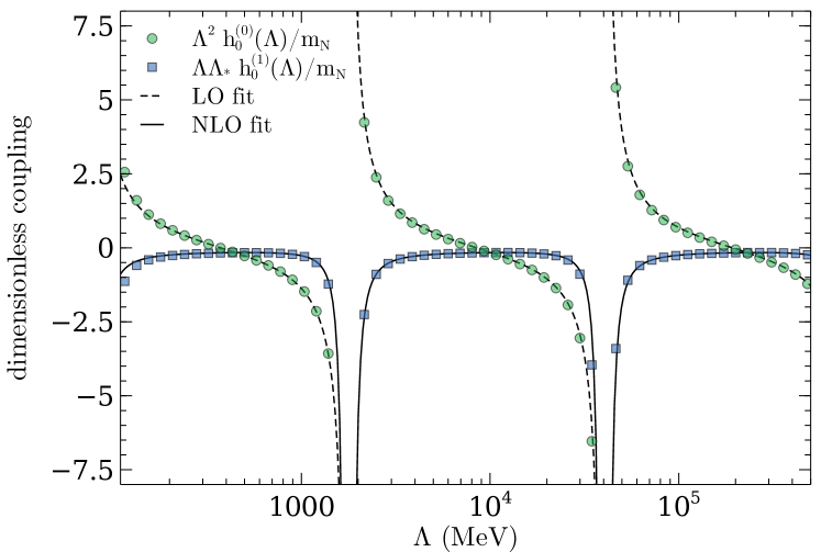
Figure 12: RG running of the three-body coupling $h_{0}$ at LO and NLO. Numerical data points are fitted using Eq. (44) at LO and an analogous expression Ji et al. (2012) at NLO.

Such a $3N$ force would be of higher order according to naïve dimensional analysis. The fact that it has to be included already at LO to renormalize the three-body system is another consequence of the fine tuning encountered in the two-body sector. After renormalization the Efimov tower of states is cutoff independent, its position determined by $\Lambda_{*}$. If the $N\!N$ scattering lengths were in fact infinite, one would have a tower of shallow three-body states accumulating at zero energy. The large but finite physical scattering lengths cut off this spectrum in the IR, whereas the breakdown scale $M_{\text{hi}}$ of the EFT sets a limit for the deepest state. In nuclear physics at physical quark masses, $a_{\rm s}$ and $m_{\pi}$ are not large enough for the appearance of an excited $3N$ state. However, Rupak et al. (2019) show, in agreement with earlier model calculations Adhikari and Tomio (1982), that a shallow virtual state in $nd$ scattering, known to exist for a long time van Oers and Seagrave (1967); Girard and Fuda (1979), becomes the first excited bound state as $a_{\rm s}$ increases. Other situations are discussed by Braaten and Hammer (2003).

The Phillips line

Pionless EFT at LO offers a striking but simple explanation of the well-known “Phillips line”, i.e., the fact that different model potentials for the nuclear interaction tuned to the same $N\!N$ scattering data give different but highly correlated results for the triton binding energy and the doublet $nd$ scattering length Phillips (1968). Pionless EFT allows one to understand this and other correlations among three-body observables as a consequence of the RG, i.e., as a correlation originating in the variation of $\Lambda_{*}$ Bedaque et al. (2000). This is shown in Fig. 13. The proximity of the LO EFT line to the experimental point means that, whichever observable is used as input, the other comes out correct.

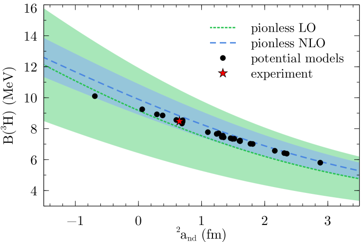
Figure 13: Correlation between the triton binding energy $B(^{3}{\mathrm{H}})$ and the doublet $nd$ scattering length ${}^{2}a_{nd}$ (Phillips line) at LO and NLO, compared to results from various potential models and experiment. Bands indicate estimates of higher-order corrections: the larger band around the dotted line is LO, the smaller band around the dashed line, NLO.

II.3.3 More neutron-deuteron scattering

Range corrections, partial resummation, and two-body parametrizations

At NLO one needs to account for the two-body ranges. In the dibaryon framework that means one insertion of each dibaryon kinetic-energy operator between LO amplitudes, as shown in Fig. 14. At N²LO, the procedure of perturbative range insertions becomes tedious, and a direct calculation of the corrections requires fully off-shell LO amplitudes. To avoid this, range corrections can be resummed with Eq. (31). Already Bedaque and van Kolck (1998) noted that this resummation introduces an artificial deep pole in the deuteron propagator. Located at a momentum scale of roughly $200\leavevmode\nobreak\ \mathrm{MeV}$, it is outside the range of validity of the EFT and thus in principle an irrelevant UV artifact, although it limits the range of cutoffs that can be used in the numerical solution of the scattering equations. This is especially true in the doublet $S$ channel unless measures are taken to remove the pole. In the quartet channel, due to the Pauli principle, the solution is not sensitive to this deep pole and the cutoff can be made arbitrarily large. Considering effective ranges as LO as proposed by Beane and Savage (2001) effectively cuts off the integral of the three-body equation at $\sim r_{0}^{-1}$, eliminating the UV limit cycle and leaving only the IR limit cycle manifest in the Efimov effect. However, in general there is no guarantee that the Efimov tower is at the correct location without a three-body force. Similar results are expected from any selective resummation of higher-order effects, such as relativistic corrections Epelbaum et al. (2017b).

$\,,\,$ $\;\sim\;\left(p_{0}-\frac{\mathbf{p}^{2}}{4m_{N}}\right)$

Figure 14: Dibaryon kinetic-energy corrections for the $nd$ quartet-channel scattering amplitude at NLO. In the doublet channel, there are analogous diagrams with ${}^{1}S_{0}$ dibaryons.

Bedaque et al. (2003b) proposed a middle ground that partially re-expands the resummed propagators and uses terms up to order $n$ for a calculation at NⁿLO. Using these “partially resummed” propagators generates all desired terms at a given order, but still retains some higher-order corrections, which have to be assumed to be negligible. We note that for such an approach to be valid it is important to keep the cutoff at or below the breakdown scale of the theory. ${}^{3}S_{1}$-${}^{3}D_{1}$ mixing as well as relativistic corrections formally enter at N²LO but were not included by Bedaque et al. (2003b). Grießhammer (2004) implemented the two-body parametrization (42) and found a substantially better description of data, particularly in the doublet $S$ wave.

The first strictly perturbative NLO calculation of $nd$ scattering in the doublet $S$ channel was carried out by Hammer and Mehen (2001a), implementing the procedure suggested by Bedaque et al. (2000). Vanasse (2013) developed a scheme that avoids the numerically expensive determination of full off-shell amplitudes made in earlier perturbative calculations Ji et al. (2012); Ji and Phillips (2013), requiring even slightly less effort than using the partial resummation of Bedaque et al. (2003b). Beyond the practical benefit, Vanasse (2013)’s N²LO calculation also showed that an anomalous (unitarity-violating) behavior of the quartet $S$-wave $nd$ phase shift above the deuteron breakup threshold, known to practitioners as a consequence of the partial-resummation scheme, does not occur with a fully perturbative treatment of range corrections. The lesson is that individually small, undesirable effects can be generated by their infinite resummation. Overall, Vanasse (2013) obtains $nd$ phase shifts at N²LO which are in good agreement with the empirical behavior up to laboratory energies of $\simeq 24\leavevmode\nobreak\ \mathrm{MeV}$.

Higher partial waves

Even with only $S$-wave interactions in the two-body sector, the nucleon-exchange diagram driving the $nd$ scattering equations (Fig. 10) generates contributions in all partial waves. Gabbiani et al. (2000) calculated the scattering phase shifts up to $G$ waves ($\ell=4$) to N²LO using the full resummation (31) but omitting ${}^{3}S_{1}$-${}^{3}D_{1}$ mixing. They found good agreement with both potential-model calculations and available experimental data up to about $140\leavevmode\nobreak\ \mathrm{MeV}$ center-of-mass momentum, indicating that the breakdown scale of Pionless EFT is indeed close to being set by the pion mass, at least for these particular observables. Better results still are obtained with the two-body parametrization (42) Grießhammer (2004). The fully perturbative N²LO calculation by Vanasse (2013) did include ${}^{3}S_{1}$-${}^{3}D_{1}$ mixing and found reasonable agreement with potential-model results.

The vector analyzing power $A_{y}$ has defied explanation with potential models even at energies as low as a few $\mathrm{MeV}$—the “$A_{y}$ puzzle”. Margaryan et al. (2016) employed the fully perturbative approach to calculate $nd$ polarization observables at N³LO. They found that varying the ${}^{3}P_{J}$ LECs (first entering at N³LO) with the expected error (a $15\%$ band around their central values) covers a range for $A_{y}$ that is consistent with experimental data.

Ordering of three-body forces

Bedaque et al. (2000) argued that at NLO range corrections force a shift in the LEC of the $3N$ force (43), which was confirmed by Hammer and Mehen (2001a) in an explicit NLO calculation. Thus,

$$h(\Lambda)=h_{0}^{(0)}(\Lambda)+h_{0}^{(1)}(\Lambda)+\cdots\,,$$ (45)

where $h_{0}^{(0)}(\Lambda)$ is given in Eq. (44) and $h_{0}^{(1)}(\Lambda)$, determined in a fully perturbative calculation with physical $N\!N$ effective-range parameters, is shown in Fig. 12. At NLO, the numerical data has been fit with the analytical result found by Ji et al. (2012). The existence of the correction $h_{0}^{(1)}$ does not mean that there is a new three-body force at NLO—it is merely an adjustment of the LO coefficient carried out by demanding that the observable used to fixed $h_{0}^{(0)}(\Lambda)$ stays invariant after the inclusion of range corrections. Because there is no new three-body parameter at NLO, simple correlations through $\Lambda_{\star}$ survive with small shifts, as can be seen in the NLO line in Fig. 13. Since $h_{0}^{(1)}(\Lambda)$ depends on the two-body scattering lengths, if the latter are changed, further experimental input is needed to determine the NLO LEC Ji et al. (2010).

The conclusion that, despite having canonical dimension 9, the nonderivative three-body force appears at LO together with the nonderivative two-body force of dimension 6 raised the questions: Do other three-body interactions have to be promoted? More generally, what is the ordering of three-body forces in the pionless power counting? Since according to Bedaque et al. (2000) a new $3N$ force enters at N²LO, Bedaque et al. (2003b) used a Lepage-plot analysis Lepage (1997) to show that its inclusion reduces the errors in the calculation. A general and comprehensive analysis of pionless three-body forces using the asymptotic techniques of Bedaque et al. (1999a, b, 2000) was carried out by Grießhammer (2005), who identified a logarithmic divergence at N²LO that mandates the inclusion of a new three-body force at this order. Grießhammer (2005) also cataloged the minimal orders at which $3N$ forces must first appear in various channels for proper renormalization. Platter and Phillips (2006), using a subtractive renormalization scheme, argued that the LO three-body force is sufficient to achieve cutoff independence up to N²LO, contradicting the findings of Bedaque et al. (2003b). Ji et al. (2012) and Ji and Phillips (2013), studying the three-boson system, later explained this discrepancy by noting that the conclusion of Platter and Phillips (2006) only holds in the limit where the three-body UV cutoff is taken to infinity, with the partial resummation of range corrections affecting the perturbative expansion at smaller cutoffs. Using a fully perturbative inclusion of range corrections, Ji and Phillips (2013) concluded that a new three-body force indeed enters at N²LO. This term can be implemented using the same $SU(4)$-symmetric spin-isospin structure as the LO three-body force, with appropriate time derivatives included to give a linear dependence on the energy Ji and Phillips (2013); Vanasse (2013).

Generalizing these results, the $3N$ potential takes the form (9) with (cf. Grießhammer (2005)) $\mu=d+2-s_{3}$, where $s_{3}=0,1,2$ is the number of nucleon-deuteron ($N\!d$) Wigner-symmetric $S$ waves connected by the operator. The first orders are represented in Fig. 5. Amplitudes have the form (5) with the normalization (20) for $A=3$.

II.3.4 Proton-deuteron scattering and helion

Nonperturbative Coulomb effects

As discussed in Sec. II.2.7, at the low energies potentially reached in scattering Coulomb-photon exchange needs to be treated nonperturbatively, which poses additional technical challenges. The first attempt to study Coulomb effects was made in the simpler quartet $S$-wave $pd$ scattering by Rupak and Kong (2003). They developed a power counting that, with some approximations, amounts to iterating a Coulomb potential between proton and deuteron to all orders, along with the one-nucleon exchange diagram that also enters in $nd$ scattering. Rupak and Kong (2003) calculated the Coulomb-subtracted $S$-wave phase shift in the quartet channel, but could not reach convergence below $pd$ center-of-mass momenta of $20\leavevmode\nobreak\ \mathrm{MeV}$ (the regime where Coulomb effects really are nonperturbative). Convergence down to $3\leavevmode\nobreak\ \mathrm{MeV}$ was later achieved by König and Hammer (2011) owing to an improved numerical procedure. König and Hammer (2011) also extended the analysis to the doublet $S$-wave channel, including helion, and applied the partial-resummation approach of Bedaque et al. (2003b) to calculate higher orders.

Ando and Birse (2010) carried out a direct momentum-space calculation of helion based on a generalization of the $nd$ integral equation discussed in Sec. II.3.2. Recasting methods developed by Kok et al. (1979, 1981) into EFT, Ando and Birse (2010) included Coulomb effects via a fully off-shell Coulomb $T$ matrix and obtained, at a single momentum cutoff $\Lambda_{0}=380.689\leavevmode\nobreak\ \mathrm{MeV}$ (the first cutoff value where the experimental triton binding energy is reproduced without a $3N$ force, $H(\Lambda_{0})=0$) a ${}^{3}\mathrm{He}$ binding energy $B({}^{3}\mathrm{He})\simeq 7.66\leavevmode\nobreak\ \mathrm{MeV}$, close to the experimental value of about $7.72\leavevmode\nobreak\ \mathrm{MeV}$. Ando and Birse (2010) treated all Coulomb effects nonperturbatively, but considered the strong sector only at LO. Kirscher et al. (2010) obtained similar numerical results in a calculation that included NLO and selected higher-order interactions as part of an effective potential which was treated exactly.

The pionless calculation of $pd$ scattering and helion was revisited and extended by König (2013) and König et al. (2015), who argued that the NLO $pd$ system, within the partial-resummation approach, is not properly renormalized by the isospin-symmetric $3N$ force alone. The same conclusion was reached in a parallel analysis by Vanasse et al. (2014), who calculated $pd$ scattering and ${}^{3}\mathrm{He}$ at NLO in strict perturbation theory. Using an asymptotic analysis, it was shown that Coulomb at LO requires a nonderivative $3N$ interaction at NLO (but not LO) to properly renormalize the $pd$ system. At this level, one can no longer predict low-energy $pd$ scattering from $nd$ scattering without further input. Fixing the corresponding LEC to the ${}^{3}\mathrm{He}$ binding energy gives good agreement with an analytically-derived expression, and it also provides cutoff-stable results for the phase shift. In contrast, Kirscher and Gazit (2016) recently argued that ${}^{3}\mathrm{He}$ is renormalized at NLO without an additional counterterm ($pd$ scattering was not investigated). While both calculations use Pionless EFT, they differ in the numerical implementation and regularization scheme.

A comparison of the different schemes for the counting of Coulomb effects in $pd$ scattering up to NLO was provided by König and Hammer (2014). These authors argued that for the scattering of composite charged particles there is a certain arbitrariness in the definition of Coulomb-subtracted quantities (phase shifts and modified ERE parameters), namely whether or not information about the deuteron substructure is included in the definition of the pure Coulomb phase shift.

Perturbative Coulomb effects

Renewed interest and developments in the strict application of perturbation theory also motivated a new look into the counting of Coulomb effects. The characteristic trinucleon momentum scale $\gamma_{T}\sim 80\leavevmode\nobreak\ \mathrm{MeV}\gg\alpha m_{N}$ suggests that Coulomb effects should be a perturbative correction to the ${}^{3}\mathrm{He}$ binding energy (compared to the triton as its isospin mirror state). Already König et al. (2015) showed that the calculation of Ando and Birse (2010) can be reproduced essentially unchanged when the fully off-shell Coulomb $T$ matrix is replaced by one-photon exchange diagrams. However, the calculation of König et al. (2015) is still nonperturbative because $B({}^{3}\mathrm{He})$ is extracted from the pole in the off-shell $pd$ amplitude obtained from an integral equation that resums both one-nucleon exchange as well as $\mathcal{O}(\alpha)$ Coulomb diagrams. König et al. (2016) instead calculated the binding-energy difference $B({}^{3}\mathrm{H})-B({}^{3}\mathrm{He})$ as a perturbation around an isospin-symmetric LO including a contribution missed in the earlier calculation of König et al. (2015). Once the logarithmic divergence generated by $pp$ Coulomb effects is isolated and properly renormalized, the NLO ${}^{3}\mathrm{He}$ binding energy converges as the cutoff increases without an isospin-breaking $3N$ force. König et al. (2016) find $B({}^{3}\mathrm{He})=(7.62\pm 0.17)\leavevmode\nobreak\ \mathrm{MeV}$, supporting the perturbative nature of Coulomb in this bound state. The same conclusion was reached independently by Kirscher and Gazit (2016). These results suggest that for nuclear ground states Coulomb is an NLO effect and isospin-breaking $3N$ forces do not enter up to this order. The same holds for $pd$ scattering for center-of-mass momenta $k\gtrsim 20\leavevmode\nobreak\ \mathrm{MeV}$, which König (2017) showed to be predicted from $nd$ scattering up to NLO.

Dineutron constraints

Kirscher and Phillips (2011) used Pionless EFT to constrain the neutron-neutron ($nn$) scattering length, for which there exist conflicting experimental determinations of ${-}16.1\pm 0.4\leavevmode\nobreak\ \mathrm{fm}$ Huhn et al. (2000, 2001) and ${-}18.7\pm 0.7\leavevmode\nobreak\ \mathrm{fm}$ Gonzalez Trotter et al. (1999, 2006). Using a model-independent correlation between the difference of the $nn$ and (Coulomb-modified) $pp$ scattering lengths on the one hand and the ${}^{3}\mathrm{H}$-${}^{3}\mathrm{He}$ binding-energy difference on the other, Kirscher and Phillips (2011) extracted $a_{nn}=(-22.9\pm 4.1)\leavevmode\nobreak\ \mathrm{fm}$ from an LO calculation where isospin-breaking, nonderivative $N\!N$ contact interactions are included.

Kirscher and Phillips (2011) only considered negative values for $a_{nn}$, thus excluding the possibility of a bound shallow state, the existence of which would correspond to $a_{nn}$ large and positive. Motivated by renewed experimental interest in the existence of such a state, Hammer and König (2014) revisited the calculation and argued that the relevant parameter that enters the pionless calculation is not $a_{nn}$ directly, but rather its inverse, such that going from large negative to large positive $a_{nn}$ is only a small change. Extending the calculation of Kirscher and Phillips (2011) to NLO, and taking into account the new $pd$ counterterm identified by Vanasse et al. (2014), Hammer and König (2014) concluded that Pionless EFT currently does not exclude a bound dineutron state.

II.3.5 Infrared regulators

Solving the EFT beyond the three-nucleon system poses significant technical challenges. All calculations so far have relied on the transition to the Hamiltonian and a solution of the Schrödinger equation or one of its many-body variants. One way to mitigate difficulties is to introduce an IR regulator in the form of a confining potential that produces discrete energy levels and, together with the UV regulator, reduces the solution of the Schrödinger equation to matrix inversion.

A simple choice is to confine the system to a periodic cubic box, as first considered for EFT by Muller et al. (2000) and Abe et al. (2004). The case of $N\!N$ in Pionless EFT was dealt with by Beane et al. (2004), where a relation between phase shifts and energy levels within the box, originally obtained by Luscher (1986, 1991), was rederived. The relations between $N\!N$ LECs and ERE parameters for a large lattice were found by Seki and van Kolck (2006). Several papers have studied the limit-cycle of the three-body system and the finite-volume corrections to three-body binding energies in periodic cubic boxes numerically Kreuzer and Hammer (2009, 2010, 2011); Kreuzer and Grießhammer (2012). An analytical expression for the volume dependence of the three-body binding energy in the unitary limit was obtained by Meißner et al. (2015) and Hansen and Sharpe (2017). König and Lee (2018) have studied the volume dependence of arbitrary $N$-body bound states, providing a more general perspective that reproduces the leading exponential dependence of the explicit three-body results just mentioned. The formulation of the three-particle quantization condition in a finite volume using the dibaryon formalism, which is required for the extraction of scattering phase shifts from lattice calculations, was considered by Briceno and Davoudi (2013), Hammer et al. (2017c), and Hammer et al. (2017b). Alternative approaches Hansen and Sharpe (2014); Mai et al. (2017) are reviewed by Hansen and Sharpe (2019). $N\!d$ scattering in the quartet $S$- and $P$-wave channels was calculated on a lattice by Elhatisari et al. (2016a), and found to be in good agreement with continuum results. Other reactions, such as $np\to d\gamma$ Rupak and Lee (2013) and $pp$ fusion Rupak and Ravi (2015), are also accessible with this method.

Another widely employed confining potential is the harmonic oscillator, which can also be deployed to EFT Stetcu et al. (2010b). The analog of the Lüscher formula, due to Busch et al. (1998), also follows from Pionless EFT Stetcu et al. (2010a); Luu et al. (2010). Using this relation to determine the two- and three-nucleon LECs from, respectively, $N\!N$ and $nd$ phase shifts, Rotureau et al. (2012) generalized an earlier calculation for spin $\nicefrac{{1}}{{2}}$ fermions Rotureau et al. (2010) and reproduced previous NLO results for two- and three-nucleons in the limit of a wide harmonic oscillator. Tölle et al. (2011, 2013) investigated the related problem of up to 6 spinless bosons in a harmonic trap and provided explicit expressions for the running coupling constants. Using smeared contact interactions, they improved the convergence of the energy levels considerably. A recent refinement of the Busch formula has been worked out by Zhang (2019).

II.3.6 Four nucleons

One of the virtues of encoding the Efimov effect in the three-body force is that its consequences for systems with more nucleons can be assessed in a model-independent way. A potential obstacle is the relatively strong binding of the $A=4$ ground state, the alpha particle (${}^{4}\mathrm{He}$), whose binding energy $B({}^{4}\mathrm{He})=28.296\leavevmode\nobreak\ \mathrm{MeV}$ can be associated with a momentum scale $\gamma_{\alpha}=\sqrt{m_{N}B({}^{4}\mathrm{He})/2}\sim 110\leavevmode\nobreak\ \mathrm{MeV}$ that is not necessarily within the realm of Pionless EFT.

The application of Pionless EFT to the four-nucleon system was initiated by Platter et al. (2005), extending their previous work on the four-boson system with large two-body scattering length Platter et al. (2004). It was found that no $4N$ force is required for renormalization at LO, i.e., the alpha-particle binding energy converges as a function of increasing UV cutoff. Low-energy four-nucleon observables are then determined at LO only by two- and three-body input parameters. This means that, as for the Phillips line (Fig. 13), Pionless EFT provides a natural explanation also for the phenomenological Tjon line Tjon (1975), an empirical correlation between $B({}^{4}\mathrm{He})$ and $B({}^{3}\mathrm{H})$. The surprising success of this LO calculation Platter et al. (2005) is apparent in Fig. 15. The renormalizability and good description of the alpha-particle binding at LO found by Platter et al. (2005) have been confirmed in other calculations, for example using the resonating-group Kirscher et al. (2010, 2015) and auxiliary-field diffusion Monte Carlo Contessi et al. (2017) methods.

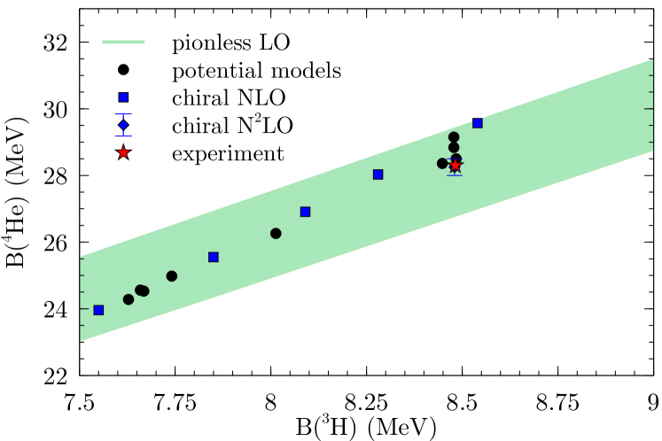
Figure 15: Correlation between alpha-particle and triton binding energies, respectively $B({}^{4}\mathrm{He})$ and $B({}^{3}\mathrm{H})$ (Tjon line), at LO in Pionless EFT, compared to results from various chiral and phenomenological potentials, and experiment. The band indicates an estimate of higher-order corrections.

Hammer and Platter (2007) later studied a four-body generalization of the Efimov effect in the four-boson system, demonstrating that the three-body ground state is associated with two four-body states, one very near the particle-trimer threshold, another deeper by a factor $\simeq 4$. The alpha-particle ground state is 3.7 times more bound than helion, and it has an excited, $0^{+}$ state just below the neutron-helion threshold. The $0^{+}$ excited state was obtained at LO by Stetcu et al. (2007), who solved the Schrödinger equation in a harmonic-oscillator basis, as done in the no-core shell model approach. The three LECs were fitted to the deuteron, triton and alpha ground-state energies, and the binding energy of the excited state, extrapolated in both UV and IR regulators, was found to be within 10% of the experimental value.

These calculations did not include the Coulomb interaction, which is consistent with the power counting developed later by König et al. (2015). Coulomb interactions have so far been included only in calculations based on effective potentials solved nonperturbatively, as suggested originally by Weinberg in the context of Chiral EFT Weinberg (1991). A variety of methods was used to solve the Schrödinger equation: resonating group Kirscher et al. (2010), stochastic variational Lensky et al. (2016), and no-core shell model Bansal et al. (2018). While results improve within a range of cutoff values, the resummation of subleading interactions (Sec. II.2.3) limits this range to small values and prevents conclusions about the RG beyond LO based on these calculations. In the first study of perturbative range corrections in $A\geq 4$ systems, Bazak et al. (2019) found that a four-body forces is required to renormalize the universal four-boson system at NLO. This result directly carries over to Pionless EFT and implies that an additional observable (most conveniently taken to be the ${}^{4}\mathrm{He}$ binding energy) is required as input at NLO to set the scale of the four-body force.

Kirscher et al. (2010) and Kirscher (2013) have pioneered the calculation of nucleon-trinucleon scattering in Pionless EFT. New correlations between the neutron-helion and neutron-triton scattering lengths, and the triton binding energy were identified. Proton-helion scattering was found in good agreement with an existing phase-shift analysis. These successes have been tempered by an LO calculation Deltuva et al. (2011) of the lowest, $0^{-}$ resonance in neutron-helion scattering—without Coulomb and an explicit $3N$ force, but with specific cutoff values for which the helion energy is correct. However, it is difficult to check the absence of regularization artifacts due to the absence of an explicit $3N$ interaction. Except for this one calculation, all evidence so far points to an unexpected triumph of the theory for $A=4$.

II.3.7 Beyond four nucleons

Nuclear binding momenta generally increase with the number of nucleons, but it is not clear what momentum scale (e.g., total binding energy or binding energy per nucleon) is most relevant for the EFT power counting. Consequently, it is an open question up to which number of nucleons Pionless EFT should work. Successful applications to ${}^{4}\mathrm{He}$, which is already significantly more deeply bound than ${}^{3}\mathrm{He}$ and ${}^{3}\mathrm{H}$, indicate that the binding energy per nucleon might be the relevant scale to estimate the binding momentum, but this remains to be firmly tested.

The first Pionless EFT calculation beyond four nucleons was carried out by Stetcu et al. (2007) with the no-core shell model. With the same parameters that led to an excellent postdiction of the ${}^{4}\mathrm{He}$ excited state, the ground-state energy of ${}^{6}\mathrm{Li}$ came out at 70% of the experimental value, which is consistent with the a priori LO uncertainty estimate from the pionless power counting. With the resonating-group method, Kirscher (2010) found that Pionless EFT does not predict a bound five-nucleon state, and carried out an exploratory study for the ${}^{6}\mathrm{He}$ system. It was concluded that Pionless EFT appears to support a shallow ${}^{6}\mathrm{He}$ bound state, but a lack of numerical convergence prevented a strong assertion.

More recently, Contessi et al. (2017) used the auxiliary-field diffusion Monte Carlo method to study ${}^{4}\mathrm{He}$ and ${}^{16}\mathrm{O}$ at LO. No evidence was found for a ${}^{16}\mathrm{O}$ that is stable with respect to breakup into four alpha particles. LO Pionless EFT does not fail to provide sufficient saturation, but a small effect such as the ${}^{16}\mathrm{O}$ energy relative to four alphas ($\sim 15\%$ of the ${}^{16}\mathrm{O}$ binding energy) requires a higher-order calculation. Bansal et al. (2018) used the coupled-cluster method to study the same systems and also ⁴⁰Ca, with qualitatively similar results at LO. With NLO interactions treated exactly, they found ${}^{16}\mathrm{O}$ and ⁴⁰Ca to be stable, and in reasonable agreement with experiment.

Leading-order calculations all show convergence with increasing cutoff in the absence of $4N$ and higher-body forces, as is the case for bosons Bazak et al. (2016). Bazak et al. (2019) show that the five- and six-boson systems are renormalized by the four-body force at NLO and conjecture that yet-higher-body forces enter at subsequent orders. For nucleons, the Pauli principle is expected to suppress these forces relative to the bosonic case because at least two derivatives are required. Together, NLO results suggest that Pionless EFT might work over a much wider range of $A$ than originally anticipated.

There have been ambitious attempts to consider even larger systems. Kirscher (2017) has recently investigated the possibility that a sufficiently large number of neutrons might bind. The properties of dilute, low-temperature neutron matter on a spacetime lattice Lee and Schäfer (2005, 2006a, 2006b); Abe and Seki (2009b, a) were found in qualitative agreement with potential-model calculations and expectations from other fermionic systems. While Pionless EFT reproduces the longstanding results for the low-density expansion in a uniform Fermi system Hammer and Furnstahl (2000), various resummations relevant for nuclear matter have been discussed by Schäfer et al. (2005), Kaiser (2011), and Kaiser (2012). Convergence of Pionless EFT at saturation density is, however, not obvious.

II.3.8 External currents and reactions

The coupling to external currents works exactly as in the two-body sector (see Sec. II.2.8). Given the increased technical challenges, there are fewer calculations, and they mostly tackle triton and helion properties. Within this limited scope, they confirm the convergence of Pionless EFT at low energies.

The simplest observable is the triton charge form factor, in particular the charge radius, which determines the leading momentum dependence. Platter and Hammer (2006) used an effective quantum-mechanical framework to obtain the form factor in the impulse approximation, i.e., considering the electric charge operator between triton wavefunctions obtained by solving a Faddeev equation for the effective potential derived from the pionless Lagrangian at LO. Similar to the Phillips line (see Sec. II.3.2), the existence of a single LO three-body parameter in Pionless EFT explains a correlation between the triton binding energy and charge radius that had previously been observed with different potential models Friar et al. (1985). An N²LO calculation was reported by Sadeghi (2010), but few details are given. Recently, the fully perturbative treatment of higher-order corrections was extended to the triton and helion charge radii at N²LO Vanasse (2017b, 2018), and magnetic moments and radii at NLO Vanasse (2018). Even though Coulomb interactions were neglected for ${}^{3}\mathrm{He}$, good agreement with experiment was found. Analogous results were obtained with a resummation of higher-order effects by Lensky et al. (2016), who also showed the correlation between the ${}^{4}\mathrm{He}$ charge radius and other three- and four-nucleon observables.

Sadeghi and Bayegan (2005), Sadeghi et al. (2006), and Sadeghi (2007) calculated the $nd\to{}^{3}\mathrm{H}\,\gamma$ capture cross section, finding good agreement with available experimental data at N²LO. Sadeghi and Bayegan (2010) calculated the inverse process of triton photodisintegration, which features the same amplitudes due to time-reversal symmetry. Several significant flaws in the calculation of Sadeghi et al. (2006) were identified by Arani et al. (2014), who presented an updated calculation. At N²LO, they still find reasonable agreement of the thermal $nd$ capture cross section with experiment. The total cross section for the related reaction $pd\to{}^{3}\mathrm{He}\,\gamma$ was calculated to NLO in a range of energies amenable to perturbative Coulomb interactions by Nematollahi et al. (2016). The $3N$ force was fixed by the helion binding energy and data were reasonably described considering the uncertainty of the calculation. The even more challenging process of deuteron-deuteron radiative capture ($dd\to{}^{4}\mathrm{He}\,\gamma$) was calculated at LO by Sadeghi and Khalili (2014), with the $3N$ force fitted to the alpha-particle energy. While available data for the astrophysical $S$-factor are apparently well described, a lack of technical details makes it difficult to assess the validity of the calculation.

New ground was broken with the extension to electroweak processes made by De-Leon et al. (2016), who studied triton $\beta$ decay to NLO. This work establishes a new way of fixing the LEC $L_{1,A}$ of the axial-vector counterpart of Eq. (41), which is relevant for other electroweak processes ($pp$ fusion, in particular) as well. Calculations like this reveal the potential of Pionless EFT to tackle interesting reactions involving more than two nucleons, based for example on the general framework developed by De-Leon et al. (2019).

II.4 Outstanding issues and current trends

Pionless EFT has fulfilled the longstanding goal of a renormalizable quantum field theory for nuclear physics. Although it has a narrow regime of strict validity, it seems to apply to, at least, $A\leq 3$ bound states and possibly to extend to $A=4$ and beyond. RG invariance, combined with the fine tuning that places two-body bound states near zero energy, has led to a power counting that flies in the face of NDA, as summarized for the potential in Fig. 5. Yet, unresolved questions remain, such as:

• How far in $A$ can we describe nuclei within this framework? So far all LO calculations ($A\leq 40$) give binding energies in agreement with experiment within the expected theoretical uncertainty, but finer details such as relative energies and thresholds are not reproduced. Calculations for $A=4,16,40$ where subleading interactions are resummed reinforce the surprising success of LO. However, at the moment, no calculation exists for more than four nucleons where NLO and higher orders are treated perturbatively. There also remain issues about the power counting of Coulomb interactions and other isospin-breaking interactions. Higher-order calculations for $A>4$ are sorely needed.

• Wigner (1937a, b) proposed an $SU(4)$ spin-isospin symmetry to explain the strong binding of nuclei containing integer numbers of alpha particles. Since the $3N$ force (43) is $SU(4)$ symmetric Bedaque et al. (2000), one cannot but wonder whether there are signs of $SU(4)$ symmetry also in light nuclei. It was shown by Chen et al. (2004b) that binding energies of $A\leq 4$ nuclei satisfy inequalities obtained from $SU(4)$ symmetry. Accordingly, Vanasse and Phillips (2017) developed an expansion around an $SU(4)$-symmetric LO based on average ${}^{1}S_{0}$ and ${}^{3}S_{1}$ scattering lengths. They showed that this expansion is promising also for observables other than binding energies, since it converges well for the triton charge radius up to NLO in the symmetry-breaking parameter (and including range corrections as well).

• In the same spirit, how far can we push the expansion around the nontrivial fixed point of the $N\!N$ amplitude, i.e., the unitary limit where both the deuteron and the ${}^{1}S_{0}$ virtual state have zero energy? In this limit the LO EFT has not only exact $SU(4)$ symmetry but also discrete scale invariance: while the two-body amplitude is invariant under continuous scale transformations Mehen et al. (2000), the three-body force (44) is symmetric only under discrete scale changes Bedaque et al. (1999a, b). This remaining symmetry leads to Efimov states in the three-body system and its descendants in the four- Hammer and Platter (2007) and higher-body systems. König et al. (2017) and König (2017), generalizing an earlier approach to the ${}^{1}S_{0}$ channel König et al. (2016), have proposed an expansion around the unitary (or unitarity) limit also in the ${}^{3}S_{1}$ channel: expansions in both $1/(Qa_{\rm t})$ and $1/(Qa_{\mathrm{s}})$ are added to the standard Pionless EFT expansion. A single LO parameter $\Lambda_{*}$ provides the nonperturbative scaffolding on top of which more quantitative results are built in by perturbation theory. This quite radical expansion appears to converge remarkably well for three- and four-nucleon binding energies König et al. (2017); König (2017). At LO all binding energies are functions of $\Lambda_{*}$, and for bosons Carlson et al. (2017) they saturate according to the liquid-drop formula. The correlation between nuclear-matter saturation energy and density expressed in the Coester line Coester et al. (1970) would emerge from variation of $\Lambda_{*}$ van Kolck (2017) just as the Tjon line—if, that is, Pionless EFT holds all the way to heavy nuclei. Related work that aims to simplify nuclear physics based on the closeness of the real world to the unitarity limit and/or Wigner $SU(4)$ limit has been carried out by Kievsky and Gattobigio (2016); Kievsky et al. (2018); Gattobigio et al. (2019); Lu et al. (2018).

III Halo/Cluster EFT

III.1 Motivation

In this section we discuss efforts to go one step further in the application of low-energy universality by including tightly bound clusters of nucleons as explicit fields in the effective Lagrangian. This Halo/Cluster EFT framework is appropriate for halo nuclei and nuclei with a cluster structure. In both cases, the energy required to remove clusters or halo nucleons, characterized by a momentum scale $M_{\text{lo}}$, is much smaller than the energy required to break clusters apart, associated with a momentum scale $M_{\text{hi}}$. The classic example is ⁶He, where the energy to separate two neutrons from an alpha-particle core is $S_{2n}\simeq 0.975\leavevmode\nobreak\ \mathrm{MeV}\ll B({}^{4}\mathrm{He})$. This class of systems can be thought of as nucleons orbiting one or more clusters, all separated by distances much larger than the cluster sizes. They typically lie at the limits of nuclear stability represented in the nuclear chart by the so-called driplines, and are target of a vigorous experimental program at rare-isotope facilities worldwide. As we discuss below, they can display more than one low-momentum scale, e.g., when Coulomb interactions are present or when a cluster has an isolated low-energy excited state.

As in Eq. (5), observables are expanded in powers of $M_{\text{lo}}/M_{\text{hi}}$ and $Q/M_{\text{hi}}$, where $Q$ is a typical momentum. While Halo/Cluster EFT is mathematically similar to the Pionless EFT for nucleons discussed in the previous section—and in fact is a theory without explicit pions by itself, becoming Pionless EFT for light nuclei when the cores are nucleons—there are a number of new aspects. First, higher partial waves between clusters, or between clusters and nucleons, are often enhanced, as for the $n\alpha$ scattering relevant for ⁶He. This causes a richer structure already in the two-body sector and requires modified power counting schemes. Second, the antisymmetrization between nucleons in a cluster (which are not active degrees of freedom) and halo nucleons is not explicit.

One might ask what kind of error is introduced by using explicit fields for tightly bound clusters. The effect on observables of exchanging nucleons in the core with halo nucleons is governed by the overlap of the wavefunctions of the halo nucleons with the wavefunctions of the core nucleons. Since the range of the former is $M_{\text{lo}}^{-1}$ while the range of the latter is $M_{\text{hi}}^{-1}$, this overlap is suppressed by $M_{\text{lo}}/M_{\text{hi}}$ compared to the overlap of two halo nucleons. Therefore, these effects are controlled by the EFT expansion in $M_{\text{lo}}/M_{\text{hi}}$ and are encoded in the LECs of Halo/Cluster EFT. The same argument applies for nucleons in different, widely separated clusters. For momenta $Q$ of the order of the breakdown scale $M_{\text{hi}}$ or above, when distances compared to the core size are probed, full antisymmetrization and other short-range physics have to be included explicitly.

Halo/Cluster EFT exploits the scale separation between $M_{\text{lo}}$ and $M_{\text{hi}}$ independently of the mechanism creating it. Thus it complements ab initio approaches to halo nuclei by zooming out to large distances and providing universal relations between different few-body observables. These relations can be combined with input from an underlying EFT or experiment to predict halo properties. Moreover, they allow us to test the consistency of different approaches and/or experiments. A particular strength lies in the possibility to describe the electroweak structure and reactions of halo nuclei in a model-independent way with controlled error estimates.

Halo/Cluster EFT can be viewed as a generalization of nuclear cluster models and is usually referred to simply as Halo EFT Bertulani et al. (2002); Bedaque et al. (2003a). We give a brief overview here, starting with $S$-wave neutron halos and Efimov states in Secs. III.2 and III.3, respectively. The complementarity with ab initio methods, useful to explore heavy halos, is discussed in Sec. III.4, before higher partial waves are tackled in Sec. III.5. We show how Halo EFT connects with electromagnetic processes in Sec. III.6, before sketching the changes needed for proton halos (Sec. III.7) and multi-cluster systems (Sec. III.8), and ending with an outlook (Sec. III.9). Our emphasis is complementary to Sec. II. A more in-depth discussion can be found in the recent review of Halo EFT by Hammer et al. (2017a).

III.2 $S$-wave neutron halos

We start with the case of $S$-wave halo nuclei or cluster states without Coulomb interactions. For definiteness, we consider one- and two-neutron halo nuclei using the formalism of Hagen et al. (2013b). The extension to other cases is straightforward. We also restrict our analysis to LO in $M_{\text{lo}}/M_{\text{hi}}$. Higher-order effects can be included as discussed in the previous section for Pionless EFT.

The effective Lagrangian for neutrons ($n$) and a spinless core ($c$) can be written as the sum of one-, two- and three-body contributions, $\mathcal{L}=\mathcal{L}_{1b}+\mathcal{L}_{2b}+\mathcal{L}_{3b}+\cdots$, where the ellipses denote higher-order terms and

$$\mathcal{L}_{1b} =\psi_{0}^{\dagger}\left(\mathrm{i}\partial_{0}+\frac{\boldsymbol{\nabla}^{2}}{2m_{0}}\right)\psi_{0}+\psi_{1}^{\dagger}\left(i\partial_{0}+\frac{\boldsymbol{\nabla}^{2}}{2m_{1}}\right)\psi_{1}\,,$$

$$\mathcal{L}_{2b} =\Delta_{1}\,d_{1}^{\dagger}d_{1}-g_{1}\left[d_{1}^{\dagger}\,(\psi_{1}\,\psi_{0})+\mathrm{H.c.}\right]$$

$$\hskip 10.00002pt\hbox{}+\Delta_{0}\,d_{0}^{\dagger}d_{0}-\frac{g_{0}}{2}\left[d_{0}^{\dagger}\,(\psi_{1}^{\text{\;T}}P\,\psi_{1})+\mathrm{H.c.}\right]\,,$$

$$\mathcal{L}_{3b} =\Omega\,t^{\dagger}\,t-h\left[t^{\dagger}(\psi_{0}\,d_{0})+(\psi_{0}\,d_{0})^{\dagger}t\right]\,.$$ (46)

The notation is slightly changed compared to the previous section (cf. Eq. (27)) in order to efficiently account for neutron and core fields, the Pauli spinor $\psi_{1}$ and the scalar $\psi_{0}$, respectively. The two-body part $\mathcal{L}_{2b}$ includes two dimerons, the scalar $d_{0}$ corresponding to an ${}^{1}S_{0}$ $nn$ pair and the Pauli spinor $d_{1}$ for a $cn$ pair. $P=\mathrm{i}\sigma_{2}/\sqrt{2}$ projects the two neutrons on the spin singlet. Finally, $\mathcal{L}_{3b}$ represents the three-body interaction written in terms of a trimeron auxiliary field Bedaque et al. (2003b), which is particularly useful for form-factor calculations Hagen et al. (2013b); Vanasse (2017b). It includes the bare trimeron residual mass $\Omega$ and the bare coupling $h$ of the trimeron $t$ to the $d_{0}$ dimeron ($nn$) and the $c$ field $\psi_{0}$. Only the parameter combination $h^{2}/\Omega$ contributes to observables at LO. As in Pionless EFT, there exists a whole class of equivalent theories with three-body forces acting in different channels. Integrating out the auxiliary fields, different choices of $\mathcal{L}_{2b}$ and $\mathcal{L}_{3b}$ can be transformed into the same theory without dimeron and trimeron fields up to four- and higher-body interactions.

In the following, we focus on the properties of the $cn$, $nn$, and $cnn$ systems. For compact notation, we define the mass parameters:

$$M_{\text{tot}}=m_{0}+2m_{1}\,,\;M_{i}=M_{\text{tot}}-m_{i}\,,\;m_{ij}=M_{i}-m_{j}\,,$$

$$\mu_{i}=\frac{m_{0}m_{1}^{2}}{m_{i}M_{i}}\,,\;\tilde{\mu}_{i}=\frac{m_{i}M_{i}}{M_{\text{tot}}}\,.$$ (47)

The diagrams for the dressed dimeron propagator, Fig. 6, are completely analogous to that for the dibaryon field discussed in Sec. II.2.5. At LO, the full dimeron propagator for the dimeron $d_{i}$ is

$$\mathrm{i}D_{i}(p_{0},\textbf{p})=\frac{2\pi\mathrm{i}}{s_{i}\,g_{i}^{2}\mu_{i}}\left[1/a_{i}-\sqrt{-2\mu_{i}\tilde{p}_{0}-\mathrm{i}\varepsilon}\,\right]^{-1}\,,$$ (48)

where $\tilde{p}_{0}=p_{0}-\textbf{p}^{2}/(2M_{i})$ and $s_{i}=\delta_{i0}/2+\delta_{i1}$ is a symmetry factor. As before, $a_{i}$ stands for the respective scattering length. For positive $a_{i}$, the propagator has a bound-state pole on the first Riemann sheet with residue $Z_{i}=2\pi/(s_{i}\,g_{i}^{2}\mu_{i}^{2}a_{i})$. For negative $a_{i}$, there is a pole on the second sheet corresponding to a virtual state.

The leading correction to the propagator (48) is due to the effective range. It can be included by making the dimeron fields dynamical as discussed in Sec. II.2.5. Here, we stay at LO in the EFT expansion and neglect effective-range corrections. The pole momentum $\gamma_{i}$ is then given by $\gamma_{i}=1/a_{i}$.

Observables in the $cnn$ system can be obtained from the $T$-matrix for the scattering process of a dimeron and a particle. The universal properties and structure of two-neutron halos were also explored in an effective quantum-mechanical framework Canham and Hammer (2008, 2010); Acharya et al. (2013) by solving the Faddeev equations for an effective potential reflecting the expansion in $M_{\text{lo}}/M_{\text{hi}}$ and for the renormalized zero-range model Amorim et al. (1997); Delfino et al. (2006). For a review of the latter work see Frederico et al. (2012).

We consider the center-of-mass frame, in which the on-shell $T$-matrix only depends on the total energy $E$ and the relative momenta in the ingoing and outgoing channels p and k, respectively. External dimeron legs are renormalized with the wavefunction renormalization factors $\sqrt{|Z_{i}|}$. The absolute value is only required for $i=0$ because $Z_{0}<0$, corresponding to the unbound $nn$ pair. Here, the factor provides a convenient redefinition of the amplitude but has no physical significance.

There are two possibilities for the initial or final state, depending on the identity of the particle and dimeron. Here we label the $T$-matrix element $T_{ij}$ by the index $i$ ($j$) of the dimeron and particle in the incoming (outgoing) channel. Keeping the matrix structure of $T_{ij}$ implicit, the integral equation for the $T$ matrix is given by Fig. 10 with the substitution in Fig. 11, where the contact three-body coupling is $h^{2}/\Omega$. The $T$ matrix can be decomposed into partial-wave contributions $T_{lm,l^{\prime}m^{\prime}}=\delta_{ll^{\prime}}\delta_{mm^{\prime}}T_{l}$. The resulting $2\times 2$-matrix integral equation for angular momentum $l$ is a generalization of the Skorniakov-Ter-Martyrosian equation Skorniakov and Ter Martirosian (1957) and reads

$$T_{l}(E,p,k)=\int_{0}^{\Lambda}\!\mathrm{d}q\,R_{l}(E,p,q)\,\bar{D}(E,q)\,T_{l}(E,q,k)\\ \hbox{}+R_{l}(E,p,k)$$ (49)

when a sharp momentum-space cutoff $\Lambda$ is imposed on the loop momentum in the three-body sector. For simplicity we focus on the $S$ wave, $l=0$, and drop the subscript $l$ on $R$ and $T$. The components of the interaction matrix $R$ are given by

$$R_{ij}(E,p,k) =\frac{2\pi\,\chi_{ij}\,m_{ij}}{\left|a_{i}a_{j}s_{i}s_{j}\right|^{\frac{1}{2}}\mu_{i}\mu_{j}}\,\frac{1}{pk}\ Q_{0}\big{(}c_{ij}\big{)}-\delta_{i0}\delta_{j0}H\,,$$

$$c_{ij} =\frac{m_{ij}}{pk}\left(\frac{p^{2}}{2\mu_{j}}+\frac{k^{2}}{2\mu_{i}}-E-\mathrm{i}\varepsilon\right)\,,$$ (50)

where $\chi_{ij}=1-\delta_{i0}\delta_{j0}$ and $Q_{0}$ is a Legendre function of the second kind. Moreover, $H=|Z_{0}|h^{2}/\Omega$ is the dimensionless three-body coupling defined in Eq. (44) which depends log-periodically on the cutoff $\Lambda$. It only contributes for angular momentum $l=0$. The dimeron matrix is diagonal in the channel indices: $\bar{D}=\text{diag}(\bar{D}_{0},\bar{D}_{1})$ with

$$\bar{D}_{i}(E,q)=\frac{\mu_{i}|a_{i}|q^{2}}{2\pi^{2}}\ \left[-1/a_{i}+\sqrt{-2\mu_{i}\tilde{E}-\mathrm{i}\varepsilon}\right]^{-1}\,,$$ (51)

and $\tilde{E}=E-q^{2}/(2\tilde{\mu}_{i})$.

The transition amplitude near the energy of an $S$-wave three-body bound state can be decomposed into a regular and an irregular part. This yields the homogeneous bound-state equation

$$\mathcal{B}(p)=\int_{0}^{\Lambda}\mathrm{d}q\,R(E,p,q)\,\bar{D}(E,q)\,\mathcal{B}(q)\,,$$ (52)

which has nontrivial solutions only at the bound-state energy $E=-B_{cnn}$.

For a given cutoff $\Lambda$, we can fix the unknown three-body parameter $H$ such that Eq. (52) has a solution at the desired value $E=-B_{cnn}$. However, any other three-body observable can be used as well. In this way, the three-body coupling is renormalized and other three-body observables (including other three-body bound states) can be predicted. In particular, Eq. (49) can be solved numerically in order to determine the $T$ matrix for three-body scattering observables. Since the two-neutron system is not bound, only the element $T_{11}$ describes a particle-dimeron scattering process, namely the scattering of a neutron from a $cn$ bound state at energy $E=p^{2}/(2\tilde{\mu}_{1})-1/(2\mu_{1}a_{1}^{2})$:

$$T_{11}\!\left(E,\,p,\,p\right)=\frac{2\pi}{\tilde{\mu}_{1}}\,\frac{1}{p\cot\delta_{cn-n}(p)-\mathrm{i}p}{\,.}$$ (53)

The other elements contribute to three-body scattering and breakup.

A fully perturbative extension of this formalism to NLO was recently presented by Vanasse (2017a). NLO equations with resummed range corrections were previously given by Canham and Hammer (2010).

III.3 Excited Efimov states in halo nuclei

The bound-state solutions of Eq. (52) are a specific variant of Efimov states Efimov (1970a, 1973). Thus the Efimov effect provides a natural binding mechanism for two-neutron halos with dominantly $S$-wave interactions. However, the contributions of higher partial waves and partial-wave mixing complicate the situation. While Halo EFT naturally accommodates resonant interactions in higher partial waves as discussed in subsection III.5, there is no Efimov effect in this case, see, e.g., Jona-Lasinio et al. (2008); Nishida (2012); Braaten et al. (2012). A general overview of Efimov states in nuclear and particle physics was given by Hammer and Platter (2010). Here, we review the possibility of identifying Efimov states in halo nuclei.

Since the strength of the interaction between the neutrons and the core is fixed, the identification of Efimov physics is more delicate than for ultracold atoms, where the effective scattering length can be dialed through an external magnetic field. In particular, the log-periodic dependence of observables on the scattering length cannot be used to identify Efimov physics. Instead one may look for excited states which (approximately) satisfy the universal scaling relation for Efimov states Efimov (1970a, 1973). Note that there are two relevant scattering lengths for a $cnn$ system, $a_{0}\equiv a_{nn}$ and $a_{1}\equiv a_{cn}$. Since $a_{nn}$ is the same for all halo nuclei and negative, we focus only on the dependence on $a_{cn}$. We define the three-body momentum as

$$K=\mathrm{sgn}(E)\sqrt{2\tilde{\mu}_{1}|E|}\,,$$ (54)

where the sign of the square root is taken as the sign of the energy $E$. The schematic dependence of the Efimov spectrum on $K$ and the inverse neutron-core scattering length $a_{cn}^{-1}$ is illustrated in Fig. 16. The breakdown scale $M_{\text{hi}}$ defines a region outside of which details of short-range physics matter and the bound states cease to be universal. Two typical situations are shown, with two universal states (at $a_{cn}>0$) and one universal state (at $a_{cn}<0$).

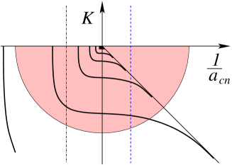
Figure 16: Illustration of the Efimov spectrum as a function of the three-body momentum $K$ (cf. Eq. (54)) and the inverse neutron-core scattering length $a_{cn}^{-1}$. The diagonal line in the fourth quadrant represents the neutron-core threshold. The solid lines indicate the Efimov states. The window of universality for bound states is represented by the hashed half circle, while the dashed and dot-dashed lines indicate a typical system with $a_{cn}>0$ and $a_{cn}<0$, respectively.

In the hypothetical unitary limit $a_{cn}^{-1}=a_{nn}^{-1}=0$, the Efimov spectrum becomes geometric,

$$K^{(n)}=-\lambda_{0}^{-n}\kappa_{*}\,,$$ (55)

where $\lambda_{0}=e^{\pi/s_{0}}$ is the discrete scaling factor and $\kappa_{*}$ is the binding momentum of the state with label $n=0$. In general, $s_{0}$ and $\lambda_{0}$ depend on the number of interacting pairs and the masses and symmetry properties of the particles, and $\lambda_{0}\approx 22.7$ for the equal-mass nucleons discussed in Sec. II. The value of $\kappa_{*}$ is related by a (regulator-dependent) constant factor to the three-body parameter $\Lambda_{\star}$ that determines the three-body force $H$ in Eq. (44). An explicit value for the case of identical bosons is given by Braaten and Hammer (2006). The spectrum shown in Fig. 16 is invariant under discrete scaling transformations with $\lambda_{0}$:

$$\kappa_{*}\longrightarrow\kappa_{*}\,,\quad a_{cn}\longrightarrow\lambda_{0}^{m}a_{cn}\,,\quad K\longrightarrow\lambda_{0}^{-m}K\,,$$ (56)

where $m$ is any integer. This discrete scale invariance holds for all few-body observables and is a clear signature of an RG limit cycle in the three-body system Bedaque et al. (1999a).

If more particles are added, no new parameters are needed for renormalization at LO Platter et al. (2004, 2005). As a consequence, all four-body observables in the universal regime are governed by the same limit cycle and can be characterized by $a$ and $\kappa_{*}$. This leads to the universal correlations between three- and four-body observables already discussed in Secs. II.3.2 and II.3.6. A similar behavior is expected for higher-body observables.

Halo nuclei have been discussed as possible candidates for Efimov states for more than 30 years Fedorov et al. (1994). As the full Efimov plot for $cnn$ systems is three-dimensional and depends on the two scattering lengths $a_{nn}$ and $a_{cn}$, it is more instructive to plot candidate nuclei in a two-dimensional plane characterized by the neutron-core energy $E_{nc}$ and the neutron-neutron energy $E_{nn}$, in units of the three-body ground-state energy $E_{gs}$, as introduced by Amorim et al. (1997). If a given nucleus lies within a certain boundary curve that weakly depends on the mass number $A$ of the core, it should display an excited Efimov state. The candidate nuclei ¹¹Li, ¹²Be, ¹⁴Be, ¹⁸C, and ²⁰C were investigated in LO Halo EFT assuming only resonant $S$-wave interactions by Canham and Hammer (2008). An update of this analysis with current halo candidates and established halo nuclei is shown in Fig. 17. The triton has also been added, since it can be interpreted as an two-neutron halo with a proton core.

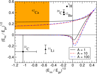
Figure 17: Boundary curves for the existence of excited Efimov states in two-neutron halo nuclei with different core masses $A$ as function of the square roots of the neutron-core energy $E_{nc}$ and neutron-neutron energy $E_{nn}$ in units of the three-body ground-state energy $E_{gs}$. The sign of the square root is taken positive (negative) if the corresponding two-body system, $nc$ or $nn$, has a bound state (virtual state). Established halo nuclei are shown by the data points while the shaded area gives the parameter range for the predicted halo nucleus ⁶²Ca. Reprinted by permission from Springer Nature: Hammer (2018), copyright (2018).

In 2010, ²²C was established as the then heaviest halo nucleus. In particular, ²²C was found to display a large matter radius Tanaka et al. (2010) and a large $S$-wave component in its $n$-²⁰C subsystem Horiuchi and Suzuki (2006). Since the information on the neutron-core energy $E_{nc}$ was ambiguous, Acharya et al. (2013) used Halo EFT to explore the correlation between the $n$-²⁰C energy and the two-neutron separation energy of ²²C. Combining this correlation with the matter-radius measurement, they demonstrated that an excited Efimov state in ²²C is unlikely. A recent update of this analysis by Hammer et al. (2017a), using the more precise matter radius from Togano et al. (2016) as input, reached the same conclusion.

Whether heavier neutron halos than ²²C exist is still an open question, although there is some experimental evidence that the ground states of ³¹Ne and ³⁷Mg have a low one-neutron separation energy and can be considered deformed $P$-wave halos Nakamura et al. (2014); Kobayashi et al. (2014). This makes it worthwhile to investigate the possibility for Efimov states in heavier nuclei.

III.4 Ab initio methods and Efimov states in heavier nuclei

Halo EFT can be used in conjunction with ab initio calculations to extend the reach of the latter or to test the consistency of different approaches. Here, we discuss an example of the former in the context of Efimov physics. Further examples regarding electromagnetic reactions will be given below.

Coupled-cluster calculations by Hagen et al. (2012b) of neutron-rich calcium isotopes—which used a chiral potential with schematic $3N$ forces and included coupling to the scattering continuum—suggested that a large $S$-wave scattering length might occur in the ⁶¹Ca system, with interesting implications for ⁶²Ca. Subsequently, Hagen et al. (2013a) computed the elastic scattering of neutrons on ⁶⁰Ca obtaining quantitative estimates for the scattering length and the effective range, and confirming that a large scattering length can be expected. These results were then used as input for Halo EFT in the study of the ⁶⁰Ca-$n$-$n$ system.

Specifically, the focus was on signals of Efimov physics that are a consequence of the large scattering lengths in the ⁶⁰Ca-$n$ and $n$-$n$ systems. This is illustrated in Fig. 18, where the universal correlation between the ⁶¹Ca-$n$ scattering length and the two-neutron separation energy of ⁶²Ca is shown. For ⁶²Ca with $m_{0}=60m_{1}$, the discrete scaling factor governing the energy spectrum is approximately $16^{2}=256$ Braaten and Hammer (2006), which is slightly more favorable than in the case of equal mass particles. The asymptotic scaling ratio applies only for deep states or in the unitary limit of infinite scattering length. Away from the unitary limit, however, the ratio of energies near threshold can be significantly smaller—see Fig. 16 and the corresponding discussion by Braaten and Hammer (2006). In the case of ⁶²Ca, the whole energy region between $S_{2n}\approx 5-8\leavevmode\nobreak\ \mathrm{keV}$ and the breakdown scale $S_{\mathrm{hi}}\approx 500\leavevmode\nobreak\ \mathrm{keV}$ is available for Efimov states. At $S_{2n}\approx 230\leavevmode\nobreak\ \mathrm{keV}$, the ⁶⁰Ca-$n$ scattering length jumps from $+\infty$ to $-\infty$ and an excited Efimov state appears. It is thus conceivable that ⁶²Ca would display an excited Efimov state and unlikely that it would not display any Efimov states at all. The matter radius of ⁶¹Ca relative to the ⁶⁰Ca core was found to be 4.9(4) $\mathrm{fm}$, while the matter radius of ⁶²Ca could be even larger, depending on the precise value of $S_{2n}$.

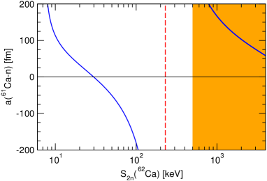
Figure 18: Correlation between the ⁶¹Ca-$n$ scattering length and the two-neutron separation energy $S_{2n}$ of ⁶²Ca. The emergence of an excited Efimov state around $S_{2n}=230$ keV is indicated by the vertical dashed line. The shaded area indicates the region where Halo EFT breaks down. Figure taken from Hammer (2016) under the terms of the Creative Commons Attribution License, https://creativecommons.org/licenses/by/4.0/.

One can summarize the situation on (excited) Efimov states in halo nuclei as follows. While the ground states of many $S$-wave halo nuclei are close to the Efimov limit, there is currently no observed halo nucleus that displays an excited Efimov state or is likely to display such a state. There is some theoretical evidence that the situation could be different for ⁶²Ca. The corresponding parameter range is indicated by the shaded square in Fig. 17. The results of Hagen et al. (2013a) imply that ⁶²Ca is possibly the largest and heaviest halo nucleus in the chart of nuclei and demonstrated that a large number of observables would display characteristic features of Efimov physics. Measurement of these observables clearly poses a significant challenge for experiment. For example, ⁵⁸Ca is the heaviest Calcium isotope that has been observed experimentally Tarasov et al. (2009). However, future radioactive-beam facilities might provide access to calcium isotopes as heavy as ⁶⁸Ca.

III.5 Higher partial waves and resonances

Next we discuss systems with resonant interactions in higher partial waves. Such interactions are ubiquitous in halo and cluster nuclei and lead to a richer power counting structure.

Consider two-body scattering with reduced mass $\mu$ and energy $E=k^{2}/2\mu$ in the center-of-mass frame. Resonance behavior arises when the $S$-matrix has a pair of poles in the two lower quadrants of the complex $k$ plane. The projection of $S$ into the resonant partial wave $l$ can be written

$$\frac{S_{l}}{s_{l}(k)}=\frac{k+k_{+}}{k-k_{+}}\,\frac{k+k_{-}}{k-k_{-}}=\frac{E-E_{0}-\mathrm{i}\Gamma(E)/2}{E-E_{0}+\mathrm{i}\Gamma(E)/2}\,.$$ (57)

Here $k_{\pm}=\pm k_{R}-\mathrm{i}k_{I}$ with $k_{R,I}>0$ are the pole positions, $s_{l}(k)$ is a smooth function in the energy region under consideration, $E_{0}=(k_{R}^{2}+k_{I}^{2})/2\mu$ is the position of the resonance (where the corresponding phase shift crosses $\pi/2$), and $\Gamma(E)/2=kk_{I}/\mu$ is referred to as the half-width of the resonance. A narrow resonance is one for which $\Gamma(E_{0})/{(2E_{0})}\ll 1$, that is, for which the poles are near the real axis, $k_{I}/k_{R}\ll 1$. We call the resonance shallow if $|k_{\pm}|\equiv M_{\text{lo}}\ll M_{\text{hi}}$. An example of a shallow, narrow resonance, is given by the ${}^{2}P_{3/2}$ resonance in $n\alpha$ scattering (the ground state of ⁵He), which has Bertulani et al. (2002) $\Gamma(E_{0})/2\simeq 0.3\leavevmode\nobreak\ \mathrm{MeV}\ll E_{0}\simeq 0.8\leavevmode\nobreak\ \mathrm{MeV}\ll E_{\alpha}\simeq 20\,\mathrm{MeV}$, or $k_{I}\simeq 6\,\mathrm{MeV}\ll k_{R}\simeq 34\leavevmode\nobreak\ \mathrm{MeV}\ll\sqrt{m_{N}E_{\alpha}}\simeq 140\leavevmode\nobreak\ \mathrm{MeV}$, where $E_{\alpha}$ is the excitation energy of the $\alpha$ core and $m_{N}$ is the nucleon mass.

Shallow resonances can be described in Halo EFT, just as bound states. For notational simplicity we take the two scattering particles to be identical, with mass $m=2\mu$ and no spin. Generalization to other situations is straightforward. Like for bound states, it is convenient to introduce a dimeron field with the quantum numbers of the resonance. Note that the formulation with dimeron fields is equivalent to a formulation with particle contact interactions. (For details see the discussion by Bertulani et al. (2002) and, for $S$-wave states, Sec. II.) In the following, we focus on the case where the resonance is in the $l=1$ state, in which case the dimeron field $d$ has three components corresponding to spin 1. In a notation similar to Eq. (27),

$${\mathcal{L}=\psi^{\dagger}\left(\mathrm{i}\partial_{0}+\frac{\boldsymbol{\nabla}^{2}}{2m}\right)\psi+d^{\dagger}_{l}\bigg{[}\eta_{1}\bigg{(}\mathrm{i}\partial_{0}+\frac{\boldsymbol{\nabla}^{2}}{4m}\bigg{)}-\Delta_{1}\bigg{]}d_{l}}\\ {\hbox{}+\frac{g_{1}}{4}\left[d^{\dagger}_{l}(\psi\tensor{\nabla}_{l}\psi)+\mathrm{H.c.}\right]+\cdots\,,}$$ (58)

where the Galilean combination $(\overset{\smash{\raisebox{-1.5pt}{\tiny$\leftarrow$}}}{\boldsymbol{\nabla}}-\overset{\smash{\raisebox{-1.5pt}{\tiny$\rightarrow$}}}{\boldsymbol{\nabla}})*=\overset{\smash{\raisebox{-1.5pt}{\tiny$\leftarrow$}}}{\boldsymbol{\nabla}}-\overset{\smash{\raisebox{-1.5pt}{\tiny$\rightarrow$}}}{\boldsymbol{\nabla}}$ places the two particles in a $P$ wave.

The full dimeron propagator, depicted in Fig. 6, is the bare propagator given by the inverse of the dimeron kinetic term and dressed by the bubbles generated by the $d\psi\psi$ interactions in Eq. (58). The two-particle $T$ matrix is obtained by attaching external particle legs. The result reproduces the ERE for $P$ waves, Eq. (LABEL:eq:T-kcot), with

$$\frac{1}{a_{1}}=\theta_{3}\Lambda^{3}-\frac{12\pi\Delta_{1}}{mg_{1}^{2}}\ \ \text{,}\ \ {-}\frac{r_{1}}{2}=\theta_{1}\Lambda+\eta_{1}\frac{12\pi}{m^{2}g_{1}^{2}}\,,$$ (59)

where, as in Eq. (22), $\theta_{1,3}$ are numbers that depend on the chosen regularization. We see that both the scattering length and effective range need to be included at LO to absorb all divergences Bertulani et al. (2002). This requirement has to be reflected by the power counting for $P$ waves. We note that the need to include additional interactions for renormalization at LO will become more severe in higher partial waves.

For the scaling of the parameters $a_{1},r_{1},\ldots$, different scenarios can be envisioned:

• Naïve dimensional analysis suggests that the typical size for the ERE parameters $a_{1},r_{1},\ldots$ is given by the appropriate power of the momentum scale $M_{\text{hi}}$ where the EFT breaks down.

For instance, if the interaction between the particles is described by a potential of depth $\sim M_{\text{hi}}$ and range $\sim 1/M_{\text{hi}}$, one would expect $a_{1}\sim 1/M_{\text{hi}}^{3}$ and $r_{1}\sim M_{\text{hi}}$. In particular, a resonance or bound state, if present, generally occurs at the momentum scale $M_{\text{hi}}$.

Scenario (i) is clearly not appropriate for halo nuclei with shallow resonances or bound states. In such systems, the interactions are finely tuned in such a way as to produce a resonance or bound state close to threshold, at a scale $M_{\text{lo}}$ much smaller than $M_{\text{hi}}$, violating the NDA estimate. This situation can occur when one or more of the ERE parameters have unnatural sizes related to $M_{\text{lo}}$.

• Bertulani et al. (2002) proposed a different power counting assuming $a_{1}\sim 1/M_{\text{lo}}^{3}$ and $r_{1}\sim M_{\text{lo}}$, while all higher ERE parameters scale with $M_{\text{hi}}$.

With this scaling, all three terms of the ERE shown explicitly in Eqs. (II.2.1) and (II.2.1) are of the same order for momenta $k\sim M_{\text{lo}}$ and must be retained at LO. Higher ERE parameters are suppressed by powers of $M_{\text{lo}}/M_{\text{hi}}$ and thus are subleading.

Scenario (ii) requires that two combinations of constants, $\Delta_{1}/g_{1}^{2}$ and $1/g_{1}^{2}$, be fine tuned against the large values $\Lambda\stackrel{{\scriptstyle>}}{{{}_{\sim}}}M_{\text{hi}}$ in Eq. (59) in order to produce a result containing powers of the small scale $M_{\text{lo}}$. From a naturalness perspective, this makes it less likely to occur in nature than a scenario with one fine tuning like the one for an $S$-wave bound state.

• An alternative scaling was suggested by Bedaque et al. (2003a), where $a_{1}\sim 1/(M_{\text{lo}}^{2}M_{\text{hi}})$, $r_{1}\sim M_{\text{hi}}$, and all other ERE parameters again scale with appropriate powers of $M_{\text{hi}}$.

This scenario requires only one combination of constants, namely $\Delta_{1}/g_{1}^{2}$, to be fine tuned.

With option (iii), the terms proportional to $1/a_{1}$ and $r_{1}k^{2}$ in the dimeron propagator are of the same order for momenta $k\sim M_{\text{lo}}$. The term stemming from the unitarity cut, $\mathrm{i}k^{3}$, is suppressed by one power of $M_{\text{lo}}/M_{\text{hi}}$ and is, therefore, subleading. The remaining terms in the ERE are even more suppressed. Thus, LO corresponds to taking the bare dimeron propagator while the effects of loops and higher-derivative interactions enter as higher-order corrections.

At LO the difference between the scalings (ii) and (iii) is the presence of the unitarity-cut term $\sim\mathrm{i}k^{3}$. This difference disappears if instead of considering generic momenta $k$ of order $M_{\text{lo}}$ we focus onto a narrow region around the position of the resonance at $k=\sqrt{2/a_{1}r_{1}}$. Due to the near cancellation within a window of size $\Delta k=2/a_{1}r_{1}^{2}$ around the pole between the two terms that are leading in scenario (iii), the unitarity-cut term has to be resummed to all orders, and provides a width to the resonance. In this kinematic range there are two fine tunings: one implicit in the short-distance physics leading to the unnatural value of $a_{1}$, and another one explicitly caused by the choice of kinematics close to the pole. Power counting for resonances is further discussed by Gelman (2009), Alhakami (2017), and Schmidt et al. (2018).

If the underlying theory cannot be solved, the appropriate scaling for a specific physical system can be inferred from the data, i.e., from the numerical values of the ERE parameters. However, such a determination is not always unique and/or different scalings might apply in different kinematic regions. In the first papers on Halo EFT, Bertulani et al. (2002) and Bedaque et al. (2003a) applied the scalings (ii) and (iii), respectively, to the lowest resonance in $n\alpha$ scattering. The experimental ERE parameters can be accommodated in both scalings such that both appear viable. Although the unitarization implicitly carried out in (iii) is not necessary except near the resonance, it improves the description throughout the low-energy region. In either case, scattering data determine the $n\alpha$ interaction parameters.

The two-neutron halo nucleus ⁶He offers a further testing ground for Halo EFT with resonant $P$ waves. The $n\alpha$ interaction in that nucleus is dominated by the ${}^{2}P_{3/2}$ resonance. The structure and renormalization of ⁶He were investigated by Rotureau and van Kolck (2012) and Ji et al. (2014). Rotureau and van Kolck (2012) calculated ⁶He at LO in the Gamow shell model using scenario (ii) and found that a three-body force—the analog of $\mathcal{L}_{3b}$ in Eq. (46)—is required to stabilize the system. Ji et al. (2014) solved the Faddeev equations in scenario (iii), but demoted the ${}^{2}S_{1/2}$ $n\alpha$ interaction to NLO. They also found that a three-body force is required for renormalization at LO and determined its running over a wide range of cutoffs. The observed behavior is not log-periodic, although some periodicity is observed. Alternative formulations at LO were investigated by Ryberg et al. (2017) and shown to be equivalent, while momentum-space probability densities of ⁶He were calculated by Göbel et al. (2019).

The power counting for resonant partial waves with $l\geq 2$ was also discussed by Bertulani et al. (2002) and Bedaque et al. (2003a). Their analysis of the power divergences of the one-loop self-energy showed that the first $l+1$ ERE parameters are required to absorb all divergences. This was confirmed by the Wilsonian RG analysis of Harada et al. (2009), which considered the cases $l=1,2$ explicitly. An alternative power counting for bound states with $l=2$ was proposed by Braun et al. (2018a) and applied to the description of $D$-wave states in ¹⁵C and ¹⁷C Braun et al. (2018b).

III.6 Electromagnetic properties and reactions

For one-neutron halos, Halo EFT essentially reproduces the ERE, but their electromagnetic structure and reactions can be predicted. The formalism is similar to that of Pionless EFT (Sec. II.3.8) and serves to illustrate it. Moreover, the accuracy limits of cluster models can be estimated from the order at which gauge-invariant couplings to currents appear.

In the following, we exemplify the power of Halo EFT in the electromagnetic sector using the example of ¹¹Be Hammer and Phillips (2011) and give a brief overview of results in other systems. The first excitation of ¹⁰Be is $3.4\leavevmode\nobreak\ \mathrm{MeV}$ above the ground state, which has $J^{P}=0^{+}$. Meanwhile, ¹¹Be has a $1/2^{+}$ state with neutron separation energy $B_{0}=500\leavevmode\nobreak\ \mathrm{keV}$, and a $1/2^{-}$ state with $2n$ separation energy $B_{1}=180\leavevmode\nobreak\ \mathrm{keV}$ Ajzenberg-Selove (1990), which we denote ¹¹Be^∗. The shallowness of these two states of ¹¹Be compared to the bound states of ¹⁰Be suggests that they have significant components in which a loosely bound neutron orbits a ¹⁰Be core. In Halo EFT, the $1/2^{+}$ state is described as an $S$-wave bound state of the neutron and the core, while $1/2^{-}$ is a $P$-wave bound state governed by scenario (iii) from the previous section.

The effective Lagrangian for the system can be obtained by combining Eq. (46) for the $1/2^{+}$ ground state and Eq. (58) (generalized to unequal masses) for the $1/2^{-}$ excited state. Photons are included via the minimal substitution, Eq. (36), and through the field strength. (See Hammer and Phillips (2011) for explicit expressions.)

Here our focus is on electric properties, and the dominant pieces of the electric response follow from the minimal substitution (36). But, at higher orders in the computation of these properties, gauge-invariant operators (counterterms) appear involving the electric field $\mathbf{E}$ and the fields $c$ for the ¹⁰Be core, $n$ for the halo neutron, $d$ for the ¹¹Be ground-state dimeron, and $d^{*}$ for the ¹¹Be^∗ excited-state dimeron. Possible one- and two-derivative operators with one power of the photon field are L_EM =  & L_C0   d^†( ∇⋅E) d + L_C0^(*)  d^*† ( ∇⋅E)  d^*
+ iL_E1^(1/2)  ( [d d^*†]_l  E_l + H.c.) + ⋯ , where $[\cdots]_{l}$ indicates the projection on $l=1$. If magnetic properties are to be considered, we have to include operators involving the magnetic field ${\bf B}$ as well.

The electric interactions in Eq. (III.6) are gauge invariant by themselves, and so we must determine the order at which they occur. Rescaling the fields to absorb all powers of $M_{\text{lo}}$ as done by Beane and Savage (2001), the scaling of the coupling constants with $M_{\text{lo}}$ can be obtained from NDA Hammer and Phillips (2011). As a consequence, the leading effects in the charge-radius-squared of the $1/2^{-}$ state in ¹¹Be are $\sim(r_{1}M_{\text{lo}})^{-1}\sim(M_{\text{lo}}M_{\text{hi}})^{-1}$. The operator proportional to $L_{C0}^{(*)}$ produces effects of order $(r_{1}M_{\text{hi}})^{-1}\sim(M_{\text{hi}})^{-2}$, and thus affects the prediction for the charge radius at NLO. Similarly, the E1($1/2^{+}\rightarrow 1/2^{-}$) matrix element has parametric dependence $M_{\text{lo}}^{-1}(M_{\text{lo}}M_{\text{hi}})^{-1/2}$. Including the proper wavefunction renormalization factors, the operator with LEC $L_{E1}^{(1/2)}$ yields an effect $\sim M_{\text{hi}}^{-1}(M_{\text{lo}}M_{\text{hi}})^{-1/2}$, and so also occurs already at NLO. Thus for electric quantities involving the shallow $1/2^{-}$ excited state of ¹¹Be there are two parameters in the Halo EFT description at NLO which cannot be fixed with ¹⁰Be-$n$ scattering information alone. There are none at LO and presumably more at N²LO.

III.6.1 Form Factors

The form factor of the ¹¹Be ground state is computed by calculating the contribution to the irreducible vertex for $A_{0}dd$ interactions shown in Fig. 19. There is no diagram coupling the photon to the neutron at this order since $Q_{n}=0$. In the Breit frame, where the four-momentum of the virtual photon is $q=(0,\mathbf{q})$, the irreducible vertex for the $A_{0}$ photon coupling to the $d$ field is ${-}\mathrm{i}eQ_{c}G_{E}(|\mathbf{q}|)$ where $Q_{c}$ is the charge of the core. A straightforward calculation yields

$$G_{E}(|\mathbf{q}|)=\frac{2\gamma_{0}}{f|\mathbf{q}|}\arctan\!\left(\frac{f|\mathbf{q}|}{2\gamma_{0}}\right)\,,$$ (60)

with $\gamma_{0}=\sqrt{\mathstrut 2\mu_{1}B_{0}}$ and $f=(1+m_{0}/m_{1})^{-1}$, in the notation of Eq. (47). For the deuteron $m_{0}=m_{N}$ and $f=1/2$, thus Eq. (60) reduces to the LO Pionless EFT result of Chen et al. (1999a).

Figure 19: The LO contribution to the irreducible vertex for an $A_{0}$ photon coupling to the ¹⁰Be-neutron $S$-wave bound state. The thick solid line indicates the ¹¹Be ground state, while the solid, dashed, and curly lines represent the neutron, ¹⁰Be core, and photon, respectively.

The form factor is a function of $\mathbf{q}^{2}$ only and the charge radius is defined as $\langle r_{E}^{2}\rangle=-6(\mathrm{d}/\mathrm{d}\mathbf{q}^{2})G_{E}|_{\mathbf{q}^{2}=0}$. Applying this expression to Eq. (60) yields

$$\langle r_{E}^{2}\rangle=\frac{f^{2}}{2\gamma_{0}^{2}}\,,$$ (61)

which gives the charge radius of the ¹¹Be ground state relative to the charge radius of ¹⁰Be. Thus we have $\langle r_{E}^{2}\rangle_{{}^{11}{\rm Be}}-\langle r_{E}^{2}\rangle_{{}^{10}{\rm Be}}=f^{2}/2\gamma_{0}^{2}$. This relation can be understood by writing the charge distribution of ¹¹Be as a convolution of the charge distribution of ¹⁰Be with that of the ¹⁰Be-$n$ halo system. Using the convolution theorem for the Fourier transform, one finds that the total mean-square radius is the sum of the squared radii for ¹⁰Be and the ¹⁰Be-$n$ halo system.

The latter effect can be calculated in Halo EFT. We note that the finite size of the core will also appear in Halo EFT at higher orders Chen et al. (1999a). An extended power-counting scheme that explicitly takes into account the scaling of the mass ratio $f$ to move these contributions to lower orders was given by Ryberg et al. (2019).

Inserting $\gamma_{0}=0.15\leavevmode\nobreak\ \mathrm{fm}^{-1}$, the relative radius becomes $\langle r_{E}^{2}\rangle_{{}^{11}{\rm Be}}-\langle r_{E}^{2}\rangle_{{}^{10}{\rm Be}}=0.19\leavevmode\nobreak\ \mathrm{fm}^{2}$. This is consistent with the experimental result, $0.51(17)\leavevmode\nobreak\ \mathrm{fm}^{2}$ Nörtershauser et al. (2009), within the $40\%$ uncertainty from NLO effects in this system. Using the experimental result for the ¹⁰Be charge radius as further input, we find $\langle r_{E}^{2}\rangle^{1/2}_{{}^{11}{\rm Be}}=2.40\leavevmode\nobreak\ \mathrm{fm}$ at LO. This is 2–3% smaller than the atomic-physics measurement which yields $\langle r_{E}^{2}\rangle^{1/2}_{{}^{11}{\rm Be}}=2.463(16)\leavevmode\nobreak\ \mathrm{fm}$ Nörtershauser et al. (2009).

At NLO a new operator associated with gauging the term $\sim d^{\dagger}\partial_{0}d$ in the effective Lagrangian contributes. The calculation produces an increased charge radius, as long as the $S$-wave $n$-¹⁰Be effective range $r_{0}$ is positive (cf. Beane and Savage (2001)),

$$\langle r_{E}^{2}\rangle_{{}^{11}{\rm Be}}-\langle r_{E}^{2}\rangle_{{}^{10}{\rm Be}}=\frac{f^{2}}{2(1-r_{0}\gamma_{0})\gamma_{0}^{2}}\,.$$ (62)

Using the value $r_{0}=2.7\leavevmode\nobreak\ \mathrm{fm}$ determined from Coulomb dissociation of ¹¹Be (see below), the relative radius becomes $\langle r_{E}^{2}\rangle_{{}^{11}{\rm Be}}-\langle r_{E}^{2}\rangle_{{}^{10}{\rm Be}}=0.31(5)\leavevmode\nobreak\ \mathrm{fm}^{2}$ at NLO, which improves the agreement with the atomic-physics measurement. The change is of order $40$%, in agreement with the a priori expectation. As a consequence, the result for the full charge radius of the ¹¹Be ground state increases to $\langle r_{E}^{2}\rangle^{1/2}_{{}^{11}{\rm Be}}=2.42\leavevmode\nobreak\ \mathrm{fm}$. In contrast to observables involving the $1/2^{-}$ state, the radius of the ¹¹Be ground state does not receive any corrections from short-distance physics until N³LO Chen et al. (1999a). The remaining difference between NLO and experimental values is consistent with the presence of the short-distance operator $\sim L_{C0}$ from Eq. (III.6) at N³LO in the expansion for the radius.

For the charge form factor of the $1/2^{-}$ excited state, NLO corrections might be expected to be smaller since its typical momentum is lower. However, a counterterm enters already at NLO for this observable. The form factor is given by the contribution to the irreducible vertex for $A_{0}d^{*}d^{*}$ interactions. There are two diagrams at LO, the first of which is analogous to that for the $1/2^{+}$ state shown in Fig. 19, while the second diagram represents a direct coupling of the photon from gauging the $d^{*\dagger}\partial_{0}d^{*}$ term in the effective Lagrangian. The latter contributes at LO because the effective range $r_{1}$ corresponds to an LO operator for the $1/2^{-}$ state. The charge form factor of the $1/2^{-}$ state at LO is obtained as Hammer and Phillips (2011)

$${G_{E}^{(*)}(|\mathbf{q}|)=1-\frac{\gamma_{1}}{r_{1}}+\frac{f^{2}\mathbf{q}^{2}+2\gamma_{1}^{2}}{|\mathbf{q}|fr_{1}}\,\arctan\!\left(\frac{f|\mathbf{q}|}{2\gamma_{1}}\right)\,,}$$ (63)

where $\gamma_{1}=\sqrt{2\mu_{1}B_{1}}$ and $r_{1}$ is the $P$-wave effective range for $n$-¹⁰Be scattering. Note that $G_{E}^{(*)}(0)=1$, as required by charge conservation, while the charge radius of the $1/2^{+}$ state relative to the ¹⁰Be ground state is

$${\langle r_{E}^{2}\rangle^{(*)}={-}\frac{5f^{2}}{2\gamma_{1}r_{1}}\,.}$$ (64)

This scales as $1/(M_{\text{lo}}M_{\text{hi}})$ as expected. It seems counterintuitive that there is a short-distance contribution to $\langle r_{E}^{2}\rangle^{(*)}$ already at NLO—especially when the corresponding effect does not occur in $\langle r_{E}^{2}\rangle$ until N³LO Chen et al. (1999a). The reason for this enhanced sensitivity is that the probability distribution of $P$-wave states is drawn in to shorter distances than the one of $S$-wave states, as it gets caught between the attractive potential that produces the $P$-wave state and the centrifugal barrier. Observables associated with a shallow $P$-wave bound state will, therefore, generically exhibit counterterms at lower order than those of their $S$-wave counterparts.

Numerical evaluation of the LO expression (64) leads to the prediction $\langle r_{E}^{2}\rangle_{{}^{11}{\rm Be}^{*}}-\langle r_{E}^{2}\rangle_{{}^{10}{\rm Be}}=0.36\leavevmode\nobreak\ \mathrm{fm}^{2}$, where we have used the value $r_{1}=-0.66\leavevmode\nobreak\ \mathrm{fm}$ from the $B(E1)$ value as input (see below). The NLO radius includes contributions from the counterterm $L_{C0}^{(*)}$ in Eq. (III.6), the coefficient of which is unknown. Hammer and Phillips (2011) estimated the NLO contributions to be of order 20%, assuming that the short-distance effects in $\langle r_{E}^{2}\rangle^{1/2}_{{}^{11}{\rm Be}^{*}}$ scale with $f$. This assumption is in agreement with the expectation from the power counting. Using again the experimental result for the ¹⁰Be charge radius Nörtershauser et al. (2009), the prediction for the charge radius of ¹¹Be^∗ at LO is $\langle r_{E}^{2}\rangle^{1/2}_{{}^{11}{\rm Be}^{*}}=(2.43\pm 0.1)\leavevmode\nobreak\ \mathrm{fm}$. To date there is no experimental determination of this charge radius.

Halo EFT calculations for the charge and magnetic form factors of ¹¹Be and ¹⁹C were performed to NLO by Fernando et al. (2015). They considered ¹⁵C as well and suggested the inclusion of the effective range as an LO effect in this particular case.

III.6.2 E1 transition and photodisintegration

Next we discuss the E1 transition from the $1/2^{+}$ state to the $1/2^{-}$ state. The irreducible vertex for this transition is depicted in Fig. 20. We compute the transition for a photon of arbitrary four momentum $k=(\omega,{\bf k})$, and the sum of diagrams yields ${-}\mathrm{i}\Gamma_{j\mu}$, where $j$ is the angular momentum index of the $d^{*}$ field and $\mu$ is the polarization index of the photon. The diagrams depicted in Fig. 20 are divergent, but their divergences cancel—providing a nontrivial check on the calculation. As long as both diagrams are considered current conservation is also satisfied Hammer and Phillips (2011), $k^{\mu}\Gamma_{j\mu}=0$. Note that if only the long-distance E1 mechanism on the left-hand side of Fig. 20 is considered—as was done, for example, by Typel and Baur (2008)—then current conservation is not satisfied and it appears that some input from short-distance physics is needed in order to define the prediction for this observable.

Figure 20: The two diagrams contributing to the irreducible vertex for the $S$-to-$P$-state transition, $\Gamma_{j\mu}$, at LO. The double line indicates the ¹¹Be excited state; the other lines are as in Fig. 19.

Evaluating the diagrams in Fig. 20, we obtain the LO Halo EFT result for ${\rm B(E1)}$,

$${\rm B(E1)}=-\frac{Z_{\text{eff}}^{2}e^{2}}{3\pi}\frac{\gamma_{0}}{r_{1}}\left[\frac{2\gamma_{1}+\gamma_{0}}{(\gamma_{0}+\gamma_{1})^{2}}\right]^{2}\,,$$ (65)

with $Z_{\text{eff}}=fQ_{c}\approx 0.366$ the effective charge. No regularization is needed in order to get a finite result. We note that the result (65) is “universal” in the sense that it applies to any E1 $S$-to-$P$-wave transition in a one-neutron halo nucleus. Once $r_{1}$, $\gamma_{1}$, and $\gamma_{0}$ are known for a given one-neutron halo, the prediction (65) is accurate up to corrections of ${\mathcal{O}}(M_{\text{lo}}/M_{\text{hi}})$.

Since there is no experimental value for the $P$-wave effective range $r_{1}$, Hammer and Phillips (2011) extracted it from the experimental number ${\rm B(E1)}(1/2^{+}\rightarrow 1/2^{-})=0.105(12)\leavevmode\nobreak\ e^{2}$ $\mathrm{fm}$² from Summers et al. (2007), yielding $r_{1}^{\rm LO}={-}0.66\leavevmode\nobreak\ \mathrm{fm}^{-1}$. Short-distance effects enter B(E1) through a counterterm in the NLO corrections. The B(E1) ($1/2^{+}\rightarrow 1/2^{-}$) transition therefore cannot be predicted at NLO, which can be seen from the presence of the operator with LEC $L^{(1/2)}_{E1}$ in Eq. (III.6).

Comparing this calculation with a shell-model treatment of ¹¹Be, it is clear that one effect which is subsumed into the NLO counterterm $L^{(1/2)}_{E1}$ is the transition of a neutron from a $d_{5/2}$ to a $p_{3/2}$ orbital, with that neutron coupled to the $2^{+}$ state of ¹⁰Be. This $2^{+}$ state is $3.4\leavevmode\nobreak\ \mathrm{MeV}$ above the ¹⁰Be ground state, so the dynamics associated with it takes place at distances $\sim M_{\text{hi}}^{-1}$. Hence in Halo EFT it can only appear in short-distance operators such as that multiplying $L^{(1/2)}_{E1}$. The computation of Millener et al. (1983) suggests that such a contribution reduces the E1 matrix element by $\sim 30$%, which is the anticipated size of an NLO effect when the $M_{\text{lo}}/M_{\text{hi}}$ expansion is employed in the ¹¹Be system. There are other effects of a similar size that will affect B(E1) at NLO. Specifically, there are NLO corrections from the wavefunction renormalization factors associated with the $S$- and $P$-wave fields. Both tend to increase B(E1) over the LO prediction.

We move on to the photodisintegration of ¹¹Be into ¹⁰Be plus a neutron. In practice this process is measured using Coulomb excitation of the ¹¹Be nucleus, with the two reactions connected within the equivalent-photon approximation. There are three contributions to this process, as depicted in Fig. 21. The first diagram, denoted “LO” in the figure, corresponds to the contribution from the plane-wave impulse approximation. The second and third diagrams, denoted “NLO”, include the final-state interactions between the neutron and the core in the $J=1/2$ channel. As we will show below, the first diagram is dominant over diagrams involving $P$-wave final-state interactions. From these diagrams, we obtain the differential B(E1) strength distribution at NLO Hammer and Phillips (2011),

$${\frac{\mathrm{d}{\rm B(E1)}}{\mathrm{d}E}=\frac{e^{2}Z_{\text{eff}}^{2}}{4\pi}\frac{12\mu_{1}\gamma_{0}{|\mathbf{p}^{\prime}}|^{3}}{\pi^{2}({\mathbf{p}^{\prime}}^{2}+\gamma_{0}^{2})^{4}}}\\ {\hbox{}\times\left(1+r_{0}\gamma_{0}+\frac{2\gamma_{0}}{3r_{1}}\frac{3{\mathbf{p}^{\prime}}^{2}+\gamma_{0}^{2}}{{\mathbf{p}^{\prime}}^{2}+\gamma_{1}^{2}}\right)\,.}$$ (66)

where ${\mathbf{p}^{\prime}}$ is is the relative momentum of the outgoing ¹⁰Be-$n$ pair and $E={\mathbf{p}^{\prime}}^{2}/(2\mu_{1})$ is the kinetic energy of the ¹⁰Be-$n$ pair in the center-of-mass frame.

Figure 21: Diagrams contributing to photodissociation of the ¹¹Be ground ($S$-wave) state. The notation is as in Fig 20.

The LO result corresponds to taking only the 1 in the parenthesis of Eq. (66). The NLO correction comes from two sources. The first is the shift of of the wavefunction renormalization to larger values due to $r_{0}>0$, which tends to increase the B(E1) strength. Second, final-state interactions between the neutron and the core in the $J=1/2$ channel enter at this order. Accurate measurements of the Coulomb dissociation spectrum therefore provide information on the $S$-wave $n$-¹⁰Be effective range, if the $P$-wave effective range is already fixed from another observable.

Up to LO accuracy for bound-to-bound state transition and NLO for bound-to-continuum, there are four LECs: $\gamma_{0}$ and $\gamma_{1}$ (which are known from separation energies) and the $S$- and $P$-wave effective ranges $r_{0}$ and $r_{1}$. At the next order, the counterterm $L_{E1}^{(1/2)}$ from Eq. (III.6) enters as well.

Folding the Halo EFT result (66) with the neutron detector resolution and the spectrum of E1 photons, the experimental data of Palit et al. (2003) are well described, as shown in Fig. 22. At NLO, if we take the value of $r_{1}$ fixed above, we have one free parameter, the value of the $S$-wave effective range $r_{0}$. A reasonable fit is found for $r_{0}=2.7\leavevmode\nobreak\ \mathrm{fm}$, very close to the effective-range result of Typel and Baur (2005) with all integrals cut off at $R=2.78\leavevmode\nobreak\ \mathrm{fm}$. This choice of the cutoff corresponds to specific assumptions about the counterterms. Another experiment by Fukuda et al. (2004) can be described equally well but suggests a 3-4% larger value for $r_{0}$.

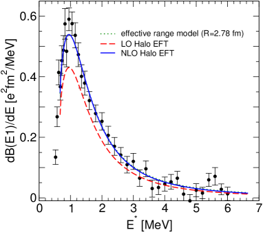
Figure 22: Differential B(E1) strength for Coulomb dissociation of ¹¹Be into ¹⁰Be + $n$ as a function of excess energy of the neutron, $E^{*}$. The dashed (solid) lines show the Halo EFT result of Hammer and Phillips (2011) at LO (NLO) folded with the detector resolution. The experimental data are from Palit et al. (2003), while the dotted line (almost on top of the solid line) gives the effective range model of Typel and Baur (2005). Reprinted from Hammer and Phillips (2011), with permission from Elsevier.

The Coulomb dissociation of the one-neutron halo nucleus ¹⁹C was studied by Acharya and Phillips (2013) using the ¹⁸C core and the neutron as effective degrees of freedom. In this case, there is no excited state present. The authors demonstrated the power of Halo EFT by calculating various observables and extracted the ERE parameters and the separation energy of the halo neutron from the Coulomb dissociation data of Nakamura et al. (1999). In particular, they obtained the values $(575\pm 55\pm 20)\leavevmode\nobreak\ \mathrm{keV}$ for the one-neutron separation energy of ¹⁹C, and $(7.75\pm 0.35\pm 0.3)\leavevmode\nobreak\ \mathrm{fm}$ for the ¹⁸C-neutron scattering length, where the first error is statistical and the second error is an estimate of the EFT uncertainty. Their prediction for the longitudinal-momentum distribution is in good agreement with the data of Bazin et al. (1995) and confirms the $S$-wave dominance for ¹⁹C.

The charge form factor and the Coulomb breakup of two-neutron halo nuclei were first calculated by Hagen et al. (2013b), Hagen (2014), and Acharya (2015) at LO. The calculation of the charge form factor was recently extended to NLO by Vanasse (2017a). (Vanasse also corrected an error in the prefactor of one term in the form factor calculation of Hagen et al. (2013b).) Since the value of the neutron-core effective range is unknown and can only be estimated, we only quote in Table 1 the LO charge radii for ¹¹Li, ¹²Be, and ²²C from Vanasse (2017a), together with the input value for the two-neutron separation energy. The charge radius for ¹¹Li has been measured by Puchalski et al. (2006) and Sanchez et al. (2006). The result $\langle r_{E}^{2}\rangle=1.104(85)$ fm² is consistent with the LO result within the estimated $40$% uncertainty due to range effects. The charge radii of ¹⁴Be and ²²C have not yet been measured.

Nucleus	$S_{2n}$ [MeV]	$\langle r^{2}_{E}\rangle$ [fm2]
11Li	0.3693(6)	0.744
14Be	1.27(13)	0.126
22C	0.11(6)	0.519 ${}^{+\infty}_{{-}0.274}$

Table 1: Two-neutron separation energies and LO charge radii squared for four different two-neutron halos. Adapted from Vanasse (2017a).

Halo EFT has also been used to calculate the matter radii of the two-neutron halos listed in Table 1 up to NLO using (i) dimeron propagators with resummed range effects Canham and Hammer (2008, 2010) and (ii) with a fully perturbative treatment of range corrections Vanasse (2017a). Both methods lead to consistent results.

III.6.3 Correlations

EFTs in general, and Halo EFT in particular, provide model-independent correlations between different observables. In Pionless EFT, the most prominent universal correlations were discussed in Secs. II.3.2 and II.3.6. Such correlations have also proven useful in the analysis of universal properties of ultracold atoms Braaten and Hammer (2006).

In the previous sections, we have expressed the electromagnetic properties of the ¹¹Be system through the ERE parameters for $n$-¹⁰Be scattering: $\gamma_{0}$, $\gamma_{1}$, $r_{0}$, and $r_{1}$. These expressions can be interpreted as correlations between scattering observables and electromagnetic properties. Analogously, there are correlations between different electromagnetic observables.

As a specific example, we consider the correlation between the B(E1) strength and the radius of the $1/2^{+}$ state in ¹¹Be at LO. Using Eqs. (64) and (65) we obtain

$${\rm B(E1)}=\frac{2e^{2}Q_{c}^{2}}{15\pi}\left(\langle r_{E}^{2}\rangle_{{}^{11}{\rm Be}^{*}}-\langle r_{E}^{2}\rangle_{{}^{10}{\rm Be}}\right)\,x\left[\frac{1+2x}{(1+x)^{2}}\right]^{2}\,,$$ (67)

where $Q_{c}$ is the charge of the core and $x=\sqrt{B_{1}/B_{0}}$ is the square root of the ratio of the neutron separation energies for the $1/2^{-}$ and $1/2^{+}$ states. The B(E1) strength is thus proportional to the mean-square radius of the $1/2^{-}$ state. In the limit of vanishing neutron separation energy for the $1/2^{-}$ state, the B(E1) strength vanishes linearly with $x$. Equation (67) can also be used to obtain the charge radius of the $1/2^{-}$ state $\langle r_{E}^{2}\rangle_{{}^{11}{\rm Be}^{*}}$ directly from the measured value of ${\rm B(E1)}$ and the neutron separation energies $B_{1}$ and $B_{0}$. This gives $\langle r_{E}^{2}\rangle_{{}^{11}{\rm Be}^{*}}-\langle r_{E}^{2}\rangle_{{}^{10}{\rm Be}}=0.35\ldots 0.39\leavevmode\nobreak\ \mathrm{fm}^{2}$, depending on which experimental value for B(E1) is used. Similar correlations can be derived for other observables.

These correlations make Halo EFT a powerful tool to test the consistency of experimental data and/or ab initio calculations based on general assumptions about the scaling of observables with $M_{\text{lo}}$ and $M_{\text{hi}}$. They can be combined with ab initio results to obtain predictions for low-energy observables as discussed in III.4 and below. In this spirit, Braun et al. (2018a) used a correlation between the B(E2) value for the transition $5/2^{+}\to 1/2^{+}$ and the quadrupole moment of the $5/2^{+}$-state in ¹⁵C to predict the quadrupole moment from ab initio calculations of the B(E2) value. Lei et al. (2018) used a correlation between the $d\alpha$ $S$-wave scattering length and the amount by which ⁶Li is bound with respect to the $np\alpha$ threshold to argue that ⁶Li is a two-nucleon halo nucleus.

III.6.4 Neutron capture

The inverse reaction of the photodissociation of one-neutron halo nuclei is radiative neutron capture on the core nucleus, which can be relevant for a variety of astrophysical processes. The corresponding efforts in Halo EFT have been reviewed by Higa (2015) and Rupak (2016).

One example is the radiative neutron capture on ⁷Li. This reaction was investigated in Halo EFT by Rupak and Higa (2011). They expressed the cross section in terms of $n$-⁷Li scattering parameters and showed that the LO uncertainty comes from the poorly known $P$-wave effective range $r_{1}$. The low-energy data for this reaction can be described well by a one-parameter fit yielding $r_{1}=-1.47\leavevmode\nobreak\ \mathrm{fm}^{-1}$. In subsequent work, Fernando et al. (2012) extended this calculation to higher energies, where the $3^{+}$ resonance becomes important. Their results suggest a resonance width about three times larger than the experimental value. They also presented power-counting arguments that establish a hierarchy for electromagnetic one- and two-body currents.

The radiative neutron capture on ⁷Li was refined by Zhang et al. (2014b) in an approach combining Halo EFT and ab initio calculations. They presented a Halo EFT calculation that describes neutron capture to both the ground and first excited states of ⁸Li. Each of the possible final states were treated as halo bound-state configurations of ⁷Li plus a neutron, including low-lying excited states of the ⁷Li core. The asymptotic normalization coefficients of these bound states were taken from an ab initio calculation using a phenomenological potential. In contrast to Rupak and Higa (2011), they found good agreement with the ratio of partial cross sections for different initial spin states. Moreover, they obtained excellent agreement with the measured branching rations between the two final states.

Rupak et al. (2012) applied Halo EFT to the dominant E1 contribution to radiative neutron capture on ¹⁴C including contributions from both resonant and non-resonant interactions. They found that significant interference between these two mechanisms leads to a capture contribution that deviates from simple Breit-Wigner resonance form.

III.7 Proton halos

Proton halos are less common due to the delicate interplay between attraction from the strong interaction and the Coulomb repulsion. The presence of the Coulomb barrier introduces the Coulomb momentum,

$${k_{C}=Z_{1}Z_{2}\alpha\mu_{12}\,,}$$ (68)

with $Z_{1,2}$ the particle charges and $\mu_{12}$ their reduced mass, as a new scale corresponding to the inverse of the Bohr radius of the system. This scale is independent of the hadronic scales and complicates the power counting (cf. the discussion for protons in Sec. II). In general, the correct scaling of the Coulomb momentum with respect to strong-interaction scales strongly depends on the system considered. One focus of recent studies in Halo EFT has been, therefore, on the underlying scaling relations in systems and reactions with Coulomb forces.

An EFT for $S$-wave proton halo nuclei was developed by Ryberg et al. (2014b). They analyzed the universal features of proton halos bound due to a large $S$-wave scattering length and derived LO expressions for the charge form factor and the radiative proton-capture cross section. In subsequent work Ryberg et al. (2016) extended the calculation to higher orders and analyzed the effect of finite-range corrections. They calculated the charge radius to NLO and the astrophysical $S$-factor for low-energy proton capture to fifth order in the low-energy expansion. Higher-order ERE parameters cannot contribute to the E1 capture reaction, and thus the accuracy is only limited by gauge-invariant counterterms. As an application, Ryberg et al. (2016) considered the $S$-factor for proton capture on ¹⁶O into the excited $1/2^{+}$ state of ¹⁷F and quantified an energy-dependent model error to be utilized in data fitting. They also provided a general discussion of the suppression of proton halos compared to neutron halos by the need for two fine tunings in the underlying theory. Schmickler et al. (2019a, b) investigated universal binding in few-body systems of up to four charged particles. They showed that range corrections are generically enhanced in the strong Coulomb case relevant for most nuclei.

The inclusion of Coulomb effects in $P$-wave halos was pioneered by Higa (2010), who looked at low-energy $p\alpha$ scattering. More extensive calculations were carried out later by Zhang et al. (2014a)—extending their previous work for neutron capture to proton halos—for ${}^{7}\mathrm{Be}(p,\gamma)^{8}\mathrm{B}$. This reaction is important for analyzing solar neutrino experiments Adelberger et al. (2011); Haxton et al. (2013). However, due to the Coulomb barrier it cannot be measured at the very low energies required for this purpose and the data must be extrapolated. Zhang et al. (2014a) demonstrated that Halo EFT together with input from ab initio calculations constitutes a powerful tool to carry out this extrapolation. They treated ${}^{8}\mathrm{B}$ as a shallow $P$-wave bound state of a proton and a ${}^{7}\mathrm{Be}$ core and included the first core excitation explicitly. The couplings were fixed using measured binding energies and $p$-${}^{7}\mathrm{Be}$ $S$-wave scattering lengths, together with ${}^{8}\mathrm{B}$ asymptotic normalization coefficients from ab initio calculations. They emphasized the important role of $p$-${}^{7}\mathrm{Be}$ scattering parameters in determining the energy dependence of $S(E)$ and demonstrated that their present uncertainties significantly limit attempts to extrapolate the data to stellar energies. Zhang et al. (2015) extended this calculation to NLO and used Bayesian methods to determine the EFT parameters and the low-energy $S$-factor, using measured cross sections and scattering lengths as inputs. The results of their analysis, which reduced the uncertainty of $S(0)$ by a factor of two, are shown in Fig. 23. Further details are given by Zhang et al. (2018a).

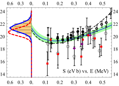
Figure 23: Right panel: NLO $S$-factor as function of energy (solid blue curve). Shading indicates 68% interval. The dashed line gives the LO result. Left panel: 1d probability distribution functions for $S(0)$ (blue line and histogram) and $S(20\leavevmode\nobreak\ \mathrm{keV})$ (red-dashed line). Figure taken from Zhang et al. (2015), under the terms of the Creative Commons Attribution License, https://creativecommons.org/licenses/by/4.0/.

In related work, Ryberg et al. (2014a) pointed out that the charge radius of ⁸B and the $S$-factor for ${}^{7}\mathrm{Be}(p,\gamma)^{8}\mathrm{B}$ are correlated at LO in Halo EFT. This correlation thus provides indirect access to the $S$-factor at low energies and serves as a consistency check.

III.8 Cluster systems

Many nuclear states are close to a threshold for break-up into smaller clusters, and are therefore amenable to an EFT approach where these smaller clusters are the relevant degrees of freedom. For example, several states of nuclei with $A=4(n+1)$, $n\geq 1$ an integer, and equal numbers of proton and neutrons are thought to be made of alpha-particle clusters Ikeda et al. (1968). The most famous example is the Hoyle state, the first $0^{+}$ excited state of ¹²C, which owing to its position near the $3\alpha$ threshold plays an important role in the creation of ¹²C and ¹⁶O—and thus our type of life—in the universe. Traditionally, these states have been investigated with a variety of phenomenological approaches Freer et al. (2018).

The first step to study these systems in Halo EFT is $\alpha\alpha$ scattering. Higa et al. (2008) developed a power counting for this system, which is highly fine tuned. Due to the subtle interplay of strong and electromagnetic forces there is a narrow resonance at an energy of about $0.1\leavevmode\nobreak\ \mathrm{MeV}$, the ⁸Be ground state. The scenario explored by Higa et al. (2008) can be viewed as an expansion around the limit where, when electromagnetic interactions are turned off, the ⁸Be ground state is at threshold and exhibits conformal invariance. This implies treating the Coulomb momentum $k_{C}=2\alpha m_{\alpha}\simeq 60$ MeV, where $m_{\alpha}$ is the alpha particle mass, as a high-momentum scale and expanding observables in powers of $Q/(3k_{C})$, where $Q$ is a typical external momentum, in addition to the standard expansion in the strong interactions. The Coulomb-modified scattering length is very large, and the corresponding effective range almost saturates the Wigner bound for charged systems König et al. (2013). The corresponding phase shifts are shown in Fig. 24 together with the experimental data from Afzal et al. (1969) and an ab initio lattice EFT calculation from Elhatisari et al. (2015). Agreement with data seems to extend somewhat beyond the laboratory energy $E_{\rm Lab}=2$ MeV corresponding to $k_{C}$. The sharp rise in the phase shift at low energies is a fine-tuned effect that is very difficult to describe in the ab initio calculation, which displays a bound state instead. In contrast, the ab initio calculation extends to much higher energies than Halo EFT.

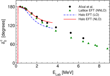
Figure 24: Halo EFT results for the $\alpha\alpha$ $S$-wave phase shift by Higa et al. (2008) as a function of the laboratory energy $E_{Lab}$. LO and NLO phase shifts are given by the (blue) dashed and (red) solid lines, respectively. The experimental data are from Afzal et al. (1969), while the lattice EFT results are from Elhatisari et al. (2015).

An RG analysis of the coupled channels $p+^{7}$Li and $n+^{7}$Be which couple to a $2^{-}$ state of ⁸Be very close to the $n+^{7}$Be threshold was carried out by Lensky and Birse (2011). A more recent study involving ⁸Be concerned a reported anomaly in the $e^{+}e^{-}$ production from the decay of one of the $1^{+}$ resonances to the ground state. A careful analysis inspired by Halo EFT was carried by Zhang and Miller (2017), who concluded that nuclear physics is unlikely to explain the experimental result.

C and O production in stars also depends on the radiative capture of alpha particles by ¹²C, ¹²C$(\alpha,\gamma)^{16}$O, at low energies. As in Sec. III.6, parameters from elastic $\alpha$-¹²C scattering enter in a Halo EFT approach to the capture process. Ando (2016, 2018) developed a description of the elastic reaction taking the ¹²C ground state as pointlike, and obtained asymptotic normalization coefficients for some of the ¹⁶O states from a fit to phase shifts.

Very little has been done using Halo EFT for other cluster systems. An early application of Halo EFT for $l=2$ to the reaction $d+t\to n+\alpha$ was carried out by Brown and Hale (2014). However, they used dimensional regularization with minimal subtraction and thus missed relevant parameters. Higa et al. (2018) recently investigated another important process in the Sun, namely the radiative capture of an $\alpha$ particle on ³He. They extracted an $S$-factor slightly above the average in the literature, but consistent within error bars. Zhang et al. (2018b) recently performed a Bayesian analysis of this reaction without relying on existing phase shift analyses as a constraint.

III.9 Outlook

In this section, we have reviewed the progress in Halo/Cluster EFT, a short-range EFT with explicit fields for nucleon and cluster degrees of freedom, designed for the description of halos and cluster nuclei. Such systems have a very rich structure due to the emergence of new scales from the Coulomb interaction between the clusters. The Efimov effect plays an important role for neutron halos and its application in the presence of Coulomb interactions presents an exciting opportunity for the discovery of new phenomena.

Halo EFT is conceptually very similar to the Pionless EFT discussed in Sec. II. As a description of nuclei not limited to the few-nucleon sector, it complements ab initio approaches by parametrizing universal relations between low-energy observables in systems dominated by shallow bound states and low-lying resonances, and it quantifies the corrections to these relations. While such ab initio calculations can be based on interactions from Chiral EFT (which is reviewed in the following section), for systems within its reach of applicability Halo EFT sets up a more effective/efficient expansion. Halo EFT promises a quantitative description on the same footing of both nuclear structure and reactions of clusterized systems and exotic isotopes, which is is a major challenge of contemporary nuclear theory. Nuclear reactions have been investigated both in strict Halo EFT Schmidt et al. (2019) as well as in accurate phenomenological models of reactions with a Halo EFT motivated description of the projectile Yang and Capel (2018); Capel et al. (2018). Many of these reactions have impact on astrophysical processes and even on the quantification of nuclear uncertainties in experimental anomalies.

Future challenges include a better integration of ab initio methods and Halo EFT in order to maximally benefit from the strengths of both approaches. The use of Bayesian statistics for the estimation of higher-order corrections provides a method to account for the different sources of theory errors beyond simple scaling arguments. Finally, hypernuclei are a new and almost unexplored arena for Halo EFT and universality. As we discuss in Sec. V.3, experimental data are not abundant and a combination of Halo EFT and ab initio methods therefore appears to be especially promising.

IV Chiral EFT

IV.1 Motivation

As the typical momentum in a nuclear process increases beyond the pion mass, pion effects can no longer be approximated by an expansion around the zero-range limit. As a response to the failure of early attempts to achieve RG invariance in pion theories, an approach gradually emerged in the 1950s where the nuclear potential and currents took purely phenomenological forms or, at best, came from the single (and, very occasionally, double) exchange of an arbitrary selection of mesons. The potential was almost always constructed so as to be regular (i.e., not a singular potential Frank et al. (1971)), which in the case of meson exchange was ensured by including physical form factors. The relative ease of solving the two-nucleon Schrödinger equation numerically made it possible to produce exquisite fits to a large amount of two-nucleon data, frequently of the same quality even with very different physical input into the potential. In contrast, a comparable description of $A>2$ systems seems to require three-nucleon forces and two-nucleon currents, but the large variety of possible structures posed a significant obstacle to this purely phenomenological approach. Moreover, the connection to QCD and the assignment of systematic errors are not addressed.

Chiral EFT attempts to overcome these shortcomings by solving the RG problems of earlier pion theories. In hindsight, the latter were both too restrictive, in the sense of not including all interactions consistent with symmetries, and not restrictive enough, in the sense of not incorporating the constraints of chiral symmetry. Early forms of mesonic Chiral Perturbation Theory (ChPT) date back to the 1960s and were extremely important in the development of the EFT paradigm. The mature version of mesonic ChPT took shape in the 1980s Weinberg (1979); Gasser and Leutwyler (1984, 1985), and processes for $A=1$ Gasser et al. (1988); Jenkins and Manohar (1991a, b); Bernard et al. (1991b, a) and $A\geq 2$ Weinberg (1990); Rho (1991); Weinberg (1991); Ordóñez and van Kolck (1992); Weinberg (1992); van Kolck (1993) started receiving significant attention in the late 1980s and early 1990s. As this section reviews, substantial progress has been made in understanding the structure of the nuclear potential and currents, but Chiral EFT has not yet produced a complete solution to the RG problems that plagued earlier pion theories.

Extensive reviews exist of Chiral EFT applications to nuclear phenomenology by, for example, van Kolck (1999a); Beane et al. (2001b); Bedaque and van Kolck (2002); Epelbaum et al. (2009); Machleidt and Entem (2011); Epelbaum and Meißner (2012). We focus here on some of the conceptual issues, which parallel those of Pionless EFT (Sec. II) and Halo/Cluster EFT (Sec. III). Chiral EFT extends Pionless EFT to processes with characteristic momentum $Q\sim M_{\text{lo}}$, where $M_{\text{lo}}\sim m_{\pi}\ll M_{\text{QCD}}$. As discussed in Sec. IV.2, the breakdown scale $M_{\text{hi}}\stackrel{{\scriptstyle<}}{{{}_{\sim}}}M_{\text{QCD}}$ depends in part on the degrees of freedom kept explicit. Section IV.2 also discusses the pertinent symmetries and Lagrangian. The nuclear potential and currents, defined in Sec. I.3, are free of the IR enhancement that leads to nuclear bound states and resonances. As a consequence, contributions to the potential can be treated similarly to contributions to amplitudes in ChPT, as discussed in Sec. IV.3. The relation to experiment via amplitudes and the more complex issue of their renormalization are reviewed in Sec. IV.4. Analogous considerations afflict reactions with external light probes such as photons and pions, which are sketched in Sec. IV.5. Section IV.6 lists some of the outstanding issues facing Chiral EFT.

IV.2 Basic elements

IV.2.1 Degrees of freedom and symmetries

By extending the Pionless EFT of Sec. II to include an isovector field $\vec{\pi}$ that collects the three charged pion states one develops a representation of QCD for $Q\sim m_{\pi}$, with $m_{\pi}$ now among the low-energy scales collectively denoted by $M_{\text{lo}}$. In this EFT, pion exchange among nucleons generates amplitudes that are no longer given by the ERE or a simple generalization thereof. Instead, there appear non-analytic functions of $Q/m_{\pi}$ in all amplitudes.

The lightness of the pions relative to other hadrons can be explained naturally if they are identified with the pseudo-Goldstone bosons of the spontaneous breaking of (approximate) chiral symmetry, $SU(2)_{\rm L}\times SU(2)_{\rm R}$ for two flavors. In the chiral limit ($\bar{m}=0$, $\varepsilon=0$, $e=0$), the QCD Lagrangian (3) has an exact chiral symmetry. In contrast, the spectrum shows only an approximate isospin symmetry, $SU(2)_{\rm V}$. Close to the chiral limit $SU(2)_{\rm L}\times SU(2)_{\rm R}$ is an approximate symmetry of Eq. (3). Pions, which have vanishing mass in the chiral limit, acquire a relatively small but non-zero common squared mass $m_{\pi}^{2}=\mathcal{O}(M_{\text{QCD}}\bar{m})$ and a square-mass splitting $\delta m_{\pi}^{2}=\mathcal{O}(\alpha M_{\text{QCD}}^{2}/4\pi,\varepsilon^{2}m_{\pi}^{4}/M_{\text{QCD}}^{2})$ between charged and neutral states.

Pions should play a special role as long as $\bar{m}\ll M_{\text{QCD}}$. In this section we consider this regime, where we integrate out all other mesons because they are expected to have masses $\mathcal{O}(M_{\text{QCD}})$. The lightest of these is the $\sigma$ with spin $S=0$ and isospin $I=0$, and a mass (half-width) $m_{\sigma}=441\leavevmode\nobreak\ \mathrm{MeV}$ ($\Gamma_{\sigma}/2=271\leavevmode\nobreak\ \mathrm{MeV}$) Caprini et al. (2006). This suggests that the EFT radius of convergence is no larger than $M_{\text{hi}}\sim\sqrt{m_{\sigma}^{2}+\Gamma_{\sigma}^{2}/4}\simeq 500\leavevmode\nobreak\ \mathrm{MeV}$. The hadronic EFT of QCD beyond this scale is not known. The problem is power counting: by NDA, interactions with derivatives will produce powers of $Q/M_{\text{QCD}}$ in amplitudes; thus, as $Q$ approaches $M_{\text{QCD}}$ all interactions are equally important. To incorporate mesons in an EFT we need an argument that, at least at a formal level, justifies treating their masses and interactions as small with respect to $M_{\text{QCD}}$. Typically this is accomplished by assuming QCD to have further approximate symmetries. For example, scale symmetry has been invoked in the context of three flavors to justify the inclusion of a scalar-isoscalar meson Crewther and Tunstall (2015) and a dynamical “vector” symmetry Georgi (1989) postulated for the $\rho$ meson. Although very interesting, such schemes have so far met with limited success, if any, away from the mesonic sector.

One must, however, consider the effects of nucleon excitations. As mentioned in Sec. I, for $Q\ll m_{N}\sim M_{\text{QCD}}$, the nucleon mass is inert. For baryon-number conserving processes, the relevant mass scale for other baryons is their mass splitting from the nucleon. The Delta isobar with $S=3/2$ and $I=3/2$ lies at $m_{\Delta}-m_{N}-i\Gamma_{\Delta}/2\simeq(270-50\mathrm{i})\leavevmode\nobreak\ \mathrm{MeV}$ Arndt et al. (2006). Although the mass difference $m_{\Delta}-m_{N}$ does not vanish in the chiral limit, it is relatively small, in line with arguments based on a large number of colors $N_{\rm c}$: when QCD is generalized to an $SU(N_{\rm c})$ gauge theory, $m_{\Delta}-m_{N}=\mathcal{O}(M_{\text{QCD}}/N_{\rm c})$. A Deltaless version of Chiral EFT exists where the Delta isobar is integrated out, but it fails before one reaches the Delta region in $A=1$ processes, which leads to relatively large errors in $A\geq 2$ systems Pandharipande et al. (2005). To increase the radius of convergence beyond $\sim\sqrt{(m_{\Delta}-m_{N})^{2}+\Gamma_{\Delta}^{2}/4}\simeq 275\leavevmode\nobreak\ \mathrm{MeV}$, one introduces Jenkins and Manohar (1991b); Hemmert et al. (1998) a heavy field $\Delta$—a four-component object in spin and isospin space with the nucleon mass $m_{N}$ removed from its rest energy. As a consequence, the Delta kinetic energy and interactions are also expanded around the non-relativistic limit. Apart from the spin/isospin structure, the main difference with respect to the nucleon is that a term linear in the mass difference $m_{\Delta}-m_{N}$ (included in $M_{\text{lo}}$) remains in the Lagrangian. Explicit Delta propagation improves the description of data beyond threshold Fettes and Meißner (2001) and enlarges the realm of Chiral EFT beyond the Delta region once the power counting is properly reformulated Pascalutsa and Phillips (2003); Long and van Kolck (2010).

Whether other nucleon excitations should be introduced in Chiral EFT is less clear. The Roper resonance Roper (1964) is special for several reasons Long and van Kolck (2011). First, its pole appears at an energy not much above the Delta, $m_{R}-m_{N}-\mathrm{i}\Gamma_{R}/2\simeq(420-80\mathrm{i})\leavevmode\nobreak\ \mathrm{MeV}$ Arndt et al. (2006). Other resonances lie at least $M_{\text{hi}}\simeq 500\leavevmode\nobreak\ \mathrm{MeV}$ above threshold—the next resonance ($S_{11}$) has a mass $m_{S_{11}}-m_{N}\simeq 500\leavevmode\nobreak\ \mathrm{MeV}$ Arndt et al. (2006)—and it is difficult to see why they should be incorporated in the EFT without the concomitant inclusion of meson resonances. Second, the Roper width is, numerically, $\Gamma_{R}\sim\Gamma_{\Delta}(m_{R}-m_{N})^{3}/(2(m_{\Delta}-m_{N})^{3})$, as expected from ChPT widths scaling as $Q^{3}/M_{\text{QCD}}^{2}$. This is not true for higher resonances, which typically have relatively smaller widths. As a consequence, the Delta and the Roper nearly saturate the Adler-Weisberger sum rule, a result which suggests that, together with the nucleon, they fall into a simple reducible representation of the chiral group Weinberg (1969); Beane and van Kolck (2005). Inclusion of an explicit Roper field Banerjee and Milana (1996); Gegelia et al. (2016) improves the convergence of Chiral EFT around the Delta resonance Long and van Kolck (2011), but it has not been systematically investigated. In the following we consider Chiral EFT with nucleon and Delta fields only.

IV.2.2 Chiral Lagrangian

The construction of the most general chiral Lagrangian is based on the theory of the non-linear realization of a symmetry Weinberg (1968); Coleman et al. (1969); Callan et al. (1969). Different parametrizations of the three-dimensional sphere $SU(2)_{\rm L}\times SU(2)_{\rm R}/SU(2)_{\rm V}=SO(4)/SO(3)\sim S^{3}$ correspond to different choices of pion fields. Observables are of course independent of this choice. Pions appear in the chiral Lagrangian always as $\vec{\pi}/f_{\pi}$, where the pion decay constant $f_{\pi}\simeq 92\leavevmode\nobreak\ \mathrm{MeV}$ is determined by the radius of $S^{3}$. Because the three pions cannot provide a linear realization of $SO(4)$, they transform non-linearly under chiral symmetry, so each term in the chiral Lagrangian is associated with an infinite tower of interactions in powers of $(\vec{\pi}/f_{\pi})^{2}$. Nucleon $N=(p\;n)^{T}$ and Delta $\Delta=(\Delta^{++}\;\Delta^{+}\;\Delta^{0}\;\Delta^{-})^{T}$ fields can be chosen to transform under chiral symmetry just as under an isospin rotation, but with an angle linear in the pion field. Covariant derivatives of the pion and baryon fields can be defined so that they transform in the same way. They are $D_{\mu}=(1-\vec{\pi}^{2}/4f_{\pi}^{2}+\cdots)\partial_{\mu}$ and $\mathcal{D}_{\mu}=\partial_{\mu}+\mathrm{i}\vec{\tau}\cdot(\vec{\pi}\times\partial_{\mu}\vec{\pi})/4f_{\pi}^{2}+\cdots$ for the pion and nucleon, respectively, where $\vec{\tau}$ are the Pauli matrices in isospin space. For the Delta, the form is the same as for the nucleon with $\vec{\tau}$ replaced by the $I=3/2$ representation of $SO(3)$. Delta-nucleon transition operators involve a set of $2\times 4$ isospin matrices $\vec{T}$. Details are given, e.g., by Ordóñez et al. (1996).

The chiral Lagrangian is automatically chiral-invariant if it is built from isospin-symmetric operators involving the baryon fields, their covariant derivatives, and the pion covariant derivative. Chiral-symmetric interactions of the pions are thus proportional to the momentum. Away from the chiral limit, quark masses and electromagnetic interactions break chiral symmetry and even the isospin subgroup. The symmetry breaking pattern is known from Eq. (3), and interactions in the EFT are constructed to behave the same way. Thus, although chiral symmetry is not exact, information about QCD is contained also in the chiral-symmetry breaking interactions. These interactions do not necessarily involve derivatives, but must be proportional to powers of the small parameters $\bar{m}/M_{\text{QCD}}$, $\varepsilon$ and $e$, as well as the coefficients of higher-dimensional operators (including violations of parity, time-reversal, and possibly baryon-number and Lorentz invariance). The parameter $\bar{m}/M_{\text{QCD}}$ can be traded for $m_{\pi}^{2}/M_{\text{QCD}}^{2}$, while $\varepsilon$ and $e$ govern isospin-breaking quantities. Electromagnetic interactions are constrained by $U(1)_{\rm em}$ gauge invariance and appear in two ways: i) between low-energy photons and other fields via chiral-covariant derivatives enlarged to be gauge-covariant as well, and via the electromagnetic field strength; ii) among hadronic fields that originate in integrating out energetic photons.

Overall, chiral symmetry and its known breaking pattern lead to a low-energy expansion because all interactions of pions among themselves or with nucleons involve derivatives (which bring powers of $Q\sim M_{\text{lo}}$ to amplitudes), powers of $m_{\pi}^{2}\sim M_{\text{lo}}^{2}$, or powers of smaller parameters. Choices of fields with different chiral-transformation properties do not change this feature, but will in general require delicate cancelations among different interactions.

As in Pionless EFT, it is most convenient to choose a heavy nucleon for which the Dirac matrices reduce to the Pauli spin matrices $\sigma$. Analogously, one can employ a heavy Delta field using the corresponding $S=3/2$ matrices. Nucleon-Delta bilinears can be constructed with $2\times 4$ spin transition matrices $S$ analogous to the isospin transition matrices $\vec{T}$. Incorporating Lorentz invariance—in an expansion in $Q/m_{N}$—is thus no more difficult in Chiral EFT than in Pionless EFT. In recent years it has become popular to use “covariant” baryon fields from which the nucleon mass is not subtracted. As any field redefinition, such choices cannot affect observables in an essential way: amplitudes obtained from different fields but the same power counting can only differ by higher-order terms. Although these differences are sometimes interpreted as an indication of the “best” field choice, they merely reflect the error of the truncation.

The baryon-number-conserving chiral Lagrangian can be split into pieces with even numbers of fermion fields, $\mathcal{L}=\mathcal{L}_{f=0}+\mathcal{L}_{f=2}+\mathcal{L}_{f\geq 4}$, where

$$\mathcal{L}_{f=0}=\frac{1}{2}\left[\left(D_{0}\vec{\pi}\right)^{2}-(\mbox{\boldmath$D$}\vec{\pi})^{2}-m_{\pi}^{2}\vec{\pi}^{2}\left(1-\frac{\vec{\pi}^{2}}{4f_{\pi}^{2}}+\cdots\right)\right]\\ \hbox{}+\cdots\,,$$ (69a)

$$\mathcal{L}_{f=2}=N^{\dagger}\left(\mathrm{i}\mathcal{D}_{0}+\frac{\mbox{\boldmath${\cal D}$}^{2}}{2m_{N}}\right)N+\frac{g_{A}}{2f_{\pi}}N^{\dagger}\vec{\tau}\mbox{\boldmath$\sigma$}N\cdot\mbox{\boldmath$D$}\vec{\pi}\\ \hbox{}+\Delta^{\dagger}\left(\mathrm{i}\mathcal{D}_{0}+m_{N}-m_{\Delta}\right)\Delta\\ +\frac{h_{A}}{2f_{\pi}}\left(N^{\dagger}\vec{T}\mbox{\boldmath$S$}\Delta+\mathrm{H.c.}\right)\cdot\mbox{\boldmath$D$}\vec{\pi}+\cdots\,,$$ (69b)

$$\mathcal{L}_{f\geq 4}={-}\frac{C_{0\textrm{t}}}{2}\left(N^{T}P_{\mathrm{t}}N\right)^{\dagger}\left(N^{T}P_{\mathrm{t}}N\right)-\frac{1}{2}\left[C_{0\textrm{s}}+D_{2\textrm{s}}m_{\pi}^{2}\left(1-\frac{\vec{\pi}^{2}}{2f_{\pi}^{2}}+\ldots\right)\right]\left(N^{T}P_{\mathrm{s}}N\right)^{\dagger}\left(N^{T}P_{\mathrm{s}}N\right)\\ \hbox{}-\frac{C_{2\textrm{s}}}{8}\Big{\{}\left(N^{T}P_{\mathrm{s}}N\right)^{\dagger}\big{[}N^{T}P_{\mathrm{s}}\mbox{\boldmath${\cal D}$}^{2}N+(\mbox{\boldmath${\cal D}$}^{2}N)^{T}P_{\mathrm{s}}N\big{]}+\mathrm{H.c.}\Big{\}}-\frac{C_{2\textrm{t}}^{\prime}}{4}\Big{[}\left(N^{T}P_{\mathrm{t}}\mbox{\boldmath${\cal D}$}N\right)^{\dagger}\cdot\left(N^{T}P_{\mathrm{t}}\mbox{\boldmath${\cal D}$}N\right)\\ \hbox{}+\left((\mbox{\boldmath${\cal D}$}N)^{T}P_{\mathrm{t}}N\right)^{\dagger}\cdot\left((\mbox{\boldmath${\cal D}$}N)^{T}P_{\mathrm{t}}N\right)\Big{]}+\frac{G_{A}}{2f_{\pi}}N^{\dagger}\!N\,N^{\dagger}\mbox{\boldmath$\sigma$}\vec{\tau}N\cdot\mbox{\boldmath$D$}\vec{\pi}-H_{0}\,N^{\dagger}\!N\,N^{\dagger}\!N\,N^{\dagger}\!N+\cdots\,,$$ (69c)

with LECs $g_{A}$, $h_{A}$, $C_{0\textrm{s,t}}$, $D_{2\textrm{s}}$, $C_{2\textrm{s}}$, $C_{2\textrm{t}}^{\prime}$, $G_{A}$, and $H_{0}$, and where we used a notation similar to Eq. (33). Only a few representative interactions are shown explicitly here, others (including more fields, derivatives, powers of $m_{\pi}^{2}$, isospin breaking, etc.) being relegated to the “$\cdots$”. Note that many terms can be written in different forms with Fierz reordering and/or field redefinitions. One can also introduce dibaryon fields as described in Sec. II.2.5 and done, for example, by Soto and Tarrus (2012) and Long (2013).

Particularly convenient for nuclear processes, where nucleon energies and momenta are of very different magnitudes, is to use field redefinitions to eliminate time derivatives of the nucleon field in favor of spatial derivatives. When interaction terms appear in the classical Lagrangian which depend on time derivatives, the effective Lagrangian obtained via the path integral of the Hamiltonian contains additional terms Charap (1970); Salam and Strathdee (1970); Honerkamp and Meetz (1971); Charap (1971); Gerstein et al. (1971). These do not vanish in general if a momentum cutoff is used. Generally, the easiest way to respect symmetries is to implement regulators as operators in the chiral Lagrangian constructed from chiral-covariant objects Slavnov (1971); Djukanovic et al. (2005); Long and Mei (2016).

If $m_{\Delta}-m_{N}$ is considered a large scale, the Delta is integrated out and appears only through LECs starting at one order higher than in the Deltaful EFT. If $m_{\pi}$ is also considered a large scale, pions are integrated out as well. Although the chiral Lagrangian formally reduces to the pionless form (33) when terms with pions and Deltas are omitted from Eq. (69), one should keep in mind that the remaining LECs depend on what degrees of freedom appear in the EFT.

IV.3 Chiral Perturbation Theory and the nuclear potential

A great advantage of EFT over earlier attempts to describe nuclear physics from field theory is its explicit focus on the regime of momenta well below the nucleon mass, where the theory splits into sectors of fixed nucleon number $A$. As pointed out in Sec. I, there are significant differences between $A\leq 1$ and $A\geq 2$ processes.

IV.3.1 Power counting

To express amplitudes in an expansion in powers of $Q/M_{\text{QCD}}$, as in Eq. (5), one needs to count powers of both $Q\sim M_{\text{lo}}$ and $M_{\text{QCD}}$. For $Q$ one first relates nucleon energies and momenta, and this relation in general depends on the sector of the theory. For $A\leq 1$, typically (but not always) $E=\mathcal{O}(Q)$, while $A\geq 2$ processes with only nucleons in external legs involve energies $E=\mathcal{O}(Q^{2}/m_{N})$. For pions, since we count $m_{\pi}$ as $M_{\text{lo}}$, $E=\mathcal{O}(Q)$. The crucial assumption in counting powers of $M_{\text{QCD}}$ is naturalness, namely that an LEC needed to eliminate cutoff dependence of a loop at a certain order has finite pieces of the same order.

For an $A\leq 1$ Feynman diagram, the various elements scale (after renormalization) as: [eq:ChPTPC] derivative &∼Q  ,
baryon, pion propagator ∼Q^-1, Q^-2  ,
(pion) loop integral ∼(4π)^-2Q^4  , where the factor of $(4\pi)^{{-}2}$ is typical of relativistic loops. The sizes of LECs can be estimated via NDA, Eq. (11). Chiral-symmetric operators depend on arbitrary powers of the reduced strong-coupling constant $g_{\rm red}=g/(4\pi)$, which for consistency should be taken as 1. NDA applied to Eq. (69a) gives $f_{\pi}=\mathcal{O}(M_{\text{QCD}}/4\pi)$, and for a generic LEC Manohar and Georgi (1984); Georgi and Randall (1986)

$$c_{i}=\mathcal{O}\left(\frac{c_{i,\text{red}}}{f_{\pi}^{f_{i}+p_{i}-2}M_{\text{QCD}}^{\Delta_{i}}}\right)\,,\quad\Delta_{i}\equiv d_{i}+f_{i}/2-2\,,$$ (70)

where $d_{i}$, $f_{i}$ and $p_{i}$ the number of, respectively, derivatives, baryon fields, and pion fields of the corresponding operator. The reduced LEC $c_{i,\text{red}}=\mathcal{O}(1)$ for a chiral-symmetric operator. NDA is consistent with the non-relativistic expansion since applied to Eq. (69b) it gives $m_{N}=\mathcal{O}(M_{\text{QCD}})$. Keeping explicit Deltas means, however, that we are taking $(m_{\Delta}-m_{N})_{\rm red}=\mathcal{O}(M_{\text{lo}}/M_{\text{QCD}})\ll 1$, as suggested by large-$N_{\rm c}$ arguments. A chiral-symmetry breaking operator stemming from the quark masses will have a reduced LEC proportional to powers of ${\bar{m}}_{\rm red}={\bar{m}}/M_{\text{QCD}}=m_{\pi}^{2}/M_{\text{QCD}}^{2}=\mathcal{O}(M_{\text{lo}}^{2}/M_{\text{QCD}}^{2})$ and $\varepsilon\stackrel{{\scriptstyle<}}{{{}_{\sim}}}\mathcal{O}(1)$, using that $m_{\pi}^{2}=\mathcal{O}(M_{\text{QCD}}\bar{m})$ when NDA is again applied to Eq. (69a). The effect of integrating out hard photons is given by powers of $e_{\rm red}^{2}=(e/(4\pi))^{2}\stackrel{{\scriptstyle<}}{{{}_{\sim}}}\mathcal{O}(M_{\text{lo}}^{3}/M_{\text{QCD}}^{3})$ van Kolck (1993, 1995) in the corresponding reduced LEC. If we take $\varepsilon=\mathcal{O}(1)$, then $c_{i,\text{red}}=\mathcal{O}(M_{\text{lo}}^{n_{i}}/M_{\text{hi}}^{n_{i}})$ where $n_{i}$ counts the powers of the low-energy scales $m_{\pi}$, $m_{\Delta}-m_{N}$ and $(e/(4\pi))^{2/3}m_{N}$. It is convenient to enlarge the definition of $d_{i}$ to include $n_{i}$ as well. The interactions displayed in Eqs. (69a) and (69b) then have $\Delta_{i}=0$, except for the nucleon recoil term $\mbox{\boldmath${\cal D}$}^{2}/2m_{N}$ with $\Delta_{i}=1$. Chiral symmetry guarantees $\Delta_{i}\geq 0$ for all interactions stemming from the terms shown explicitly in Eq. (3).

Using standard identities for connected graphs, a diagram with $L$ loops and $V_{i}$ vertices with chiral index $\Delta_{i}$ contributes to the amplitude (5) a term with Weinberg (1979)

$$\nu=2L+\sum_{i}V_{i}\Delta_{i}\,,\quad\mathcal{N}=f_{\pi}^{4-3A-E_{b}}\,,$$ (71)

where $E_{b}$ is the number of external bosons. The factor $2L$ implies that ChPT amplitudes are in general perturbative, i.e., the non-analytic functions $F^{(\nu)}$ in Eq. (5) can be obtained from a finite number of Feynman diagrams. Because of the way NDA was inferred, these loop diagrams are accompanied by higher-index interactions that provide the necessary counterterms for RG invariance in the sense of Eq. (7). Because of chiral symmetry, $\nu\geq 0$. LO ($\mathcal{O}({\mathcal{N}})$) and NLO (relative $\mathcal{O}(Q/M_{\text{QCD}})$) consist of tree-level ($L=0$) diagrams made out of interactions with chiral index $\Delta=0$ and, respectively, no or one interaction with $\Delta=1$. They are equivalent to ancient current algebra. Baryons are not only nonrelativistic, but also approximately static. Quantum-mechanical corrections ($L\geq 1$) start at N²LO (relative $\mathcal{O}(Q^{2}/M_{\text{QCD}}^{2})$). As $\nu$ increases, progressively more short-range physics is included, which account for details of hadron structure. Many good reviews of ChPT exist, see for example Bernard et al. (1995); Bernard (2008).

That is not to say that within certain regions of phase space perturbation theory does not break down. The power counting (71) is only meant as a general rule, which is bound to fail in specific situations. For example, within a momentum window of size $\mathcal{O}(Q^{3}/M_{\text{QCD}}^{2})$ around the Delta pole—where $E\simeq m_{\Delta}-m_{N}$—the one-loop diagrams that make for most of the Delta width become important and a resummation is necessary at LO Pascalutsa and Phillips (2003); Long and van Kolck (2010). Similarly, around certain points below threshold where energies are $\mathcal{O}(Q^{2}/M_{\text{QCD}})$, nucleon recoil needs to be resummed and elevated to LO Lv and Long (2016). The latter resummation is naturally incorporated by the use of non-heavy baryon (“covariant”) fields Becher and Leutwyler (1999); Fuchs et al. (2003), but in the literature it is often wrongly implied that such a choice is necessary. In general, the choice of fields is unimportant, but one should always ensure that the power counting (71) applies to the kinematic region of interest. Any resummation needs to be done carefully so as not to break RG invariance.

Nucleon-only $A\geq 2$ processes have $E=\mathcal{O}(Q^{2}/m_{N})$ and require a resummation as well Weinberg (1991). We will return to this in Sec. IV.4, focusing for now on the sum of “irreducible” diagrams involving $A\geq 2$ nucleons (and $E_{b}=0$), which is defined (see Sec. I.3) as the “full” nuclear potential. The analogous currents are briefly discussed in Sec. IV.5.

By construction, the potential is free of IR enhancement, and we expect a power counting similar to ChPT’s to apply as long as interactions with $f\geq 4$ also obey NDA. A complication is that the full potential introduced in Sec. I.3 includes disconnected diagrams. Each disconnected piece scales as $(4\pi)^{n}Q^{-4}$, where $n$ is an integer, coming from the fact that the extra four-dimensional delta function, which enforces momentum conservation, also eliminates a loop integral. Weinberg and others Weinberg (1991); Ordóñez and van Kolck (1992); Weinberg (1992); van Kolck (1993) assumed $n=2$ on the basis of Eq. (IV.3.1), while Friar (1997) took $n=1$, which is consistent with the nonrelativistic nature of reducible loops as discussed in Sec. IV.4.3. As a consequence, a diagram with $1\leq C\leq A-1$ separately connected pieces contributes to the potential (9) with Weinberg (1991); Friar (1997) μ&= n (A-1-C) + 2L + ∑_i V_i Δ_i  ,
~N = (4π)^(2-n)Af_π^4-3A  . This power counting (with $n=2$) has been used in most studies of chiral potentials to date.

IV.3.2 Nuclear potential

In Chiral EFT, Fig. 2 is undone: pion exchange appears explicitly in the potential, with the remaining contact interactions accounting for higher-momentum physics. In contrast to Pionless EFT, the potential itself involves (irreducible) loops, where energies are comparable to momenta and nucleons are approximately static. The long-range pion-exchange contributions appear in all partial waves and yield many-body forces consistent with $2N$ forces and the hadronic physics described by ChPT. They are not known to violate the estimate (IV.3.1).

Pion loops also generate short-range contributions that cannot be separated from contact interactions in the potential. The piece of a LEC that removes the cutoff dependence in irreducible loops, or more generally the piece that obeys NDA, is sometimes referred to as a “primordial counterterm” Long and Yang (2012a, b). This is to distinguish it from another piece that renormalizes the reducible loops of the full amplitude. This additional piece may violate NDA and be present at a lower order than the primordial piece, as discussed in Sec. IV.4. As in Pionless EFT, the potential is not cutoff independent.

Leading order

The full LO potential has maximum $C$ ($C_{\rm max}=A-1$, from $A-2$ disconnected lines): it consists of the sum over pairs of the $2N$ potential at tree level ($L=0$) constructed entirely from $\Delta=0$ interactions. The long-range $2N$ potential consists of static one-pion exchange (OPE) and the primordial counterterms are the two LECs of the non-derivative chiral-symmetric contact interactions in Eq. (69c):

$$V^{(0)}=-\frac{4\pi}{m_{N}M_{N\!N}}\frac{\vec{\tau}_{1}\cdot\vec{\tau}_{2}}{\mbox{\boldmath$q$}^{2}+m_{\pi}^{2}}\left(S_{12}(\mbox{\boldmath$q$})-\frac{m_{\pi}^{2}}{3}\mbox{\boldmath$\sigma$}_{1}\cdot\mbox{\boldmath$\sigma$}_{2}\right)\\ +{C_{0\mathrm{s}}P_{\mathrm{s}}+C_{0\mathrm{t}}P_{\mathrm{t}}}\,,$$ (72)

where the indices 1 and 2 label the two nucleons, $q$ is the transferred momentum, and $S_{12}(\mbox{\boldmath$q$})=(\mbox{\boldmath$\sigma$}_{1}\cdot\mbox{\boldmath$q$})(\mbox{\boldmath$\sigma$}_{2}\cdot\mbox{\boldmath$q$})-\mbox{\boldmath$q$}^{2}(\mbox{\boldmath$\sigma$}_{1}\cdot\mbox{\boldmath$\sigma$}_{2})/3$ is the tensor operator. OPE is static because the transferred energy, related to nucleon recoil, is small (relative $\mathcal{O}(Q/M_{\text{QCD}})$) compared to $|\mbox{\boldmath$q$}|$. The scale that controls the OPE strength, in a form we can compare with short-range interactions in Pionless EFT, is given by Kaplan et al. (1998a, b):

$$M_{N\!N}=\frac{16\pi f_{\pi}^{2}}{g_{A}^{2}m_{N}}=\mathcal{O}(f_{\pi}){\,,}$$ (73)

using NDA. OPE gives rise in coordinate space to i) a tensor potential that is as singular $\sim 1/r^{3}$ as $r\to 0$, and ii) the regular Yukawa potential. The tensor potential is non-vanishing only for total spin $s=1$ and can mix waves with $l=j\pm 1$. It is attractive in some uncoupled waves like ${}^{3}P_{0}$ and ${}^{3}D_{2}$, and in one of the eigenchannels of each coupled wave. The Yukawa potential is attractive in isovector (isoscalar) channels for $s=0$ ($s=1$). The other two terms in Eq. (72) are contact interactions, which for large cutoffs contribute only to the ${}^{3}S_{1}$ and ${}^{1}S_{0}$ channels. A contact interaction from OPE has been eliminated through the redefinition

$$C_{0\mathrm{s}}+\frac{4\pi}{m_{N}M_{N\!N}}\to C_{0\mathrm{s}}=\mathcal{O}\left(\frac{4\pi}{m_{N}M_{N\!N}}\right)\,.$$ (74)

Subleading orders

The order increases as the chiral index $\Delta$, the number of loops $L$, and the number of nucleons in connected pieces increase. In much of the literature the potential at relative $\mathcal{O}(Q^{\mu}/M_{\text{QCD}}^{\mu})$ is referred to as N^μ-1LO, but this notation is not flexible enough to accommodate changes in the power counting described in Set. IV.4, which suggest $n=1$ in Eq. (IV.3.1) and also departures from NDA. For clarity, we denote the order of contributions using their explicit scaling throughout the rest of this section. The structure of the long-range nuclear potential is shown schematically in Fig. 25.

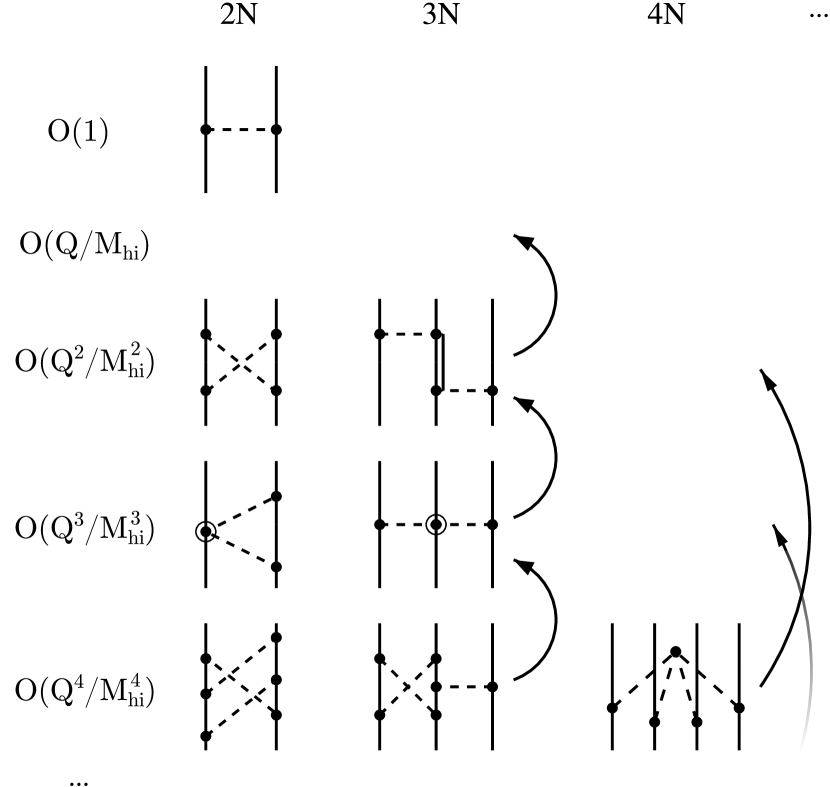
Figure 25: Sample of diagrams representing the pion-range components of the $AN$ nuclear potential in Chiral EFT, according to Eq. (IV.3.1) with $n=2$. The order of the contributions is indicated as $\mathcal{O}(Q^{\mu}/M_{\text{hi}}^{\mu})$, $\mu\geq 0$, where $Q\sim m_{\pi}$ and $M_{\text{hi}}\sim M_{\text{QCD}}$. Arrows in the $3N$ and $4N$ columns indicate the changes for $n=1$. A solid (double) line stands for a nucleon (nucleon excitation), while a dashed line, for a pion. A circle around the central solid circle denotes an inverse power of $M_{\text{hi}}$.

The first few-body forces arise van Kolck (1993, 1994) at $\mathcal{O}(Q^{n}/M_{\text{QCD}}^{n})$ compared to LO, from $\Delta=0$ and $L=0$ with $C=A-2$:

• a $3N$ TPE force via an intermediate Delta—the Fujita-Miyazawa force Fujita and Miyazawa (1957), shown in Fig. 25;

• nucleon-only $3N$ and “double-pair” forces (for $A\geq 4$) when, in a time-ordered diagram, a $2N$ interaction occurs while a pion is flying between two nucleons.

Forces of the second type exactly cancel against nucleon recoil in the $2N$ OPE, once the latter is inserted in the Lippmann-Schwinger equation Weinberg (1991); Ordóñez and van Kolck (1992); van Kolck (1993, 1994). But recoil is an $\mathcal{O}(Q/m_{N})$ effect compared to LO: the cancellation implies that $(4\pi)^{2-n}Q^{2}/M_{\text{QCD}}^{2}\sim Q/m_{N}$. For $n=2$ one obtains $Q/m_{N}\sim Q^{2}/M_{\text{QCD}}^{2}$ at variance with the NDA that underlies the power counting. In contrast, if one takes NDA seriously, $m_{N}=\mathcal{O}(M_{\text{QCD}})=\mathcal{O}(4\pi f_{\pi})$, then $n=1$ and $Q\sim f_{\pi}=\mathcal{O}(M_{NN})$. As we discuss in Sec. IV.4, this is consistent with the counting of factors of $4\pi$ suggested by Pionless EFT. Not all authors count $m_{N}$, and thus implicitly choose $n$, in the same way. However, regardless of how $m_{N}$ is counted, Chiral EFT, just as Pionless EFT, implements the constraints of Lorentz invariance in a $Q/m_{N}$ expansion.

After this cancellation, the $2N$ potential vanishes at relative $\mathcal{O}(Q/M_{\text{QCD}})$ if we neglect parity violation Weinberg (1991); Ordóñez and van Kolck (1992); van Kolck (1993, 1994). For $n=1$, the Fujita-Miyazawa $3N$ force survives at this order. It is demoted to relative $\mathcal{O}(Q^{2}/M_{\text{QCD}}^{2})$ if $n=2$, in which case the full potential vanishes at $\mathcal{O}(Q/M_{\text{QCD}})$. More generally, the first $aN$ force ($L=0$, all interactions with $\Delta=0$) is expected to appear at relative $\mathcal{O}(Q^{n(a-2)}/M_{\text{QCD}}^{n(a-2)})$. The relative suppression of few-body forces Weinberg (1991); Ordóñez and van Kolck (1992); van Kolck (1993, 1994) is in agreement with the experience drawn from phenomenological potentials containing explicit pion exchange, for which $3N$ forces are usually found necessary at the 10% level—for example, to provide $\sim 1$ MeV to the triton binding energy $\simeq 8.5\leavevmode\nobreak\ \mathrm{MeV}$. The explanation for the smallness, but non-negligibility, of phenomenological few-body forces was an early success of Chiral EFT.

$2N$ potential

At relative $\mathcal{O}(Q^{2}/M_{\text{QCD}}^{2})$, corrections to OPE merely shift existing couplings—for example, $g_{A}$ in Eq. (73) receives a contribution proportional to $m_{\pi}^{2}$, the so-called Goldberger-Treiman discrepancy. The long-range $2N$ potential consists of two-pion exchange (TPE), the so-called box, crossed-box (shown in Fig. 25), triangle and football diagrams built out of $\pi N^{\dagger}N$ and $2\pi N^{\dagger}N$ interactions with chiral index $\Delta=0$. For the latter three types, all combinations of nucleons and Deltas need to be considered in intermediate states. For the box diagram with nucleons only, once-iterated OPE needs to be subtracted. The primordial counterterms consist of all possible two-derivative chiral-symmetric contact interactions Ordóñez and van Kolck (1992); van Kolck (1993); Ordóñez et al. (1996), such as the $C_{2\mathrm{s}}$ and $C_{2\mathrm{t}}^{\prime}$ terms in Eq. (69c), and no-derivative chiral-symmetry breaking terms linear in the quark masses, such as $D_{2\mathrm{s}}$. The constraints imposed by relativity on these primordial counterterms have been discussed by Girlanda et al. (2010).

At relative $\mathcal{O}(Q^{3}/M_{\text{QCD}}^{3})$, apart from further contributions to OPE parameters, the $2N$ potential is made up of TPE with one $\Delta=1$ vertex, such as the triangle diagram shown in Fig. 25. For $n=1$, Galilean corrections ($\propto m_{N}^{-1}$) should be kept, while for $n=2$ they contribute only at next order. There are no new contact interactions at this order.

The isospin-symmetric $2N$ potential up to $\mathcal{O}(Q^{3}/M_{\text{QCD}}^{3})$ was derived early on Ordóñez and van Kolck (1992); van Kolck (1993); Ordóñez et al. (1996); Kaiser et al. (1997, 1998) and rederived many times since. Epelbaum et al. (1998) introduced the unitary transformation method which allows for the separation of the iterated OPE with a consistent set of $1/m_{N}$ corrections. Friar (1999) discusses the various forms, including pre-EFT results, and the issues involved in the separation of iterated OPE. The potential at this order resembles phenomenological potentials where pion exchange is supplemented by a short-range structure. The TPE part, which carries information about the chiral symmetry of QCD, involves LECs that can be determined from pion-nucleon scattering. (For recent work, see Hoferichter et al. (2015a); Siemens et al. (2017).) It is a chiral analog of the van der Waals potential and behaves at short distances as $1/r^{5}$, $1/r^{6}$, or $1/r^{7}$ depending on order and number of intermediate Deltas, and has the qualitative features of heavier-meson exchange potentials Kaiser et al. (1997, 1998). The TPE from Chiral EFT without explicit Deltas successfully replaces heavier-meson exchange in the Nijmegen partial-wave analysis of $2N$ data Rentmeester et al. (1999, 2003); for a modern version, see Navarro Pérez et al. (2014, 2015).

The $2N$ potential has now been extended to higher orders. One- and two-loop TPE and two-loop three-pion exchange (see Fig. 25) diagrams at $\mathcal{O}(Q^{4}/M_{\text{QCD}}^{4})$ were calculated by Kaiser (2000a, b, 2001a, 2002, 2015). More recently the long-range Deltaless potential has been constructed at $\mathcal{O}(Q^{5}/M_{\text{QCD}}^{5})$ Kaiser (2001b); Epelbaum et al. (2015c); Entem et al. (2015a), and even $\mathcal{O}(Q^{6}/M_{\text{QCD}}^{6})$ Entem et al. (2015a). By parity conservation, primordial counterterms only appear at even orders.

$3N$ potential

Beyond the Fujita-Miyazawa term, $3N$ forces have a similar hierarchy. At $\mathcal{O}(Q^{n+1}/M_{\text{QCD}}^{n+1})$, the $3N$ potential contains TPE diagrams where one interaction has $\Delta=1$ (see Fig. 25). Again, the form of TPE is constrained by chiral symmetry, and provides a chiral-corrected version of the earlier Tucson-Melbourne (TM) potential Coon et al. (1979), sometimes called the TM^′ potential Friar et al. (1999); Huber et al. (2001); Coon and Han (2001), and close in form to the Brazil potential Coelho et al. (1983). There are no additional isospin-symmetric contributions from Deltas Epelbaum et al. (2008a), but there are mixed one-pion/short-range and purely short-range components originating in the interactions with LECs $G_{A}$ and $H_{0}$, respectively, in Eq. (69c) van Kolck (1994); Epelbaum et al. (2002b). Again, parity conservation implies primordial counterterms only at every second order.

The primordial counterterms at $\mathcal{O}(Q^{n+3}/M_{\text{QCD}}^{n+3})$ have been listed by Girlanda et al. (2011). Relativistic corrections, which appear at this order for $n=1$, have been calculated by Bernard et al. (2011). At $\mathcal{O}(Q^{n+2}/M_{\text{QCD}}^{n+2})$ the first loops in the $3N$ force appear as indicated in Fig. 25, and have been derived without Deltas by Ishikawa and Robilotta (2007) and Bernard et al. (2008, 2011). The long-range Deltaless and Deltaful potentials at one order higher ($\mathcal{O}(Q^{n+3}/M_{\text{QCD}}^{n+3})$) are found in Krebs et al. (2012, 2013, 2018).

One must as well look into higher-order double-pair or other disconnected diagrams where more than two clusters of nucleons interact at the same time. Epelbaum (2006b, 2007) finds that double-pair diagrams with a recoil correction ($\mathcal{O}(Q^{2n}/M_{\text{QCD}}^{2n})$), with one insertion of a $\Delta=2$ interaction ($\mathcal{O}(Q^{n+2}/M_{\text{QCD}}^{n+2})$), or with $L=1$ ($\mathcal{O}(Q^{n+2}/M_{\text{QCD}}^{n+2})$) all add to nothing without Deltas.

$4N$ potential

Four-body forces first appear at relative $\mathcal{O}(Q^{2n}/M_{\text{QCD}}^{2n})$, among them the one from a four-pion interaction displayed in Fig. 25. They are all of long range and contain no free parameters. The components without Deltas can be found in Epelbaum (2006b, 2007). A first estimate Rozpedzik et al. (2006) of the effect of these components in ⁴He gives an additional binding of a few hundred keV. The first contact $4N$ force is of $\mathcal{O}(Q^{2(n+1)}/M_{\text{QCD}}^{2(n+1)})$; since it has no derivatives, the exclusion principle allows only one such interaction, as has been verified explicitly by Girlanda et al. (2011).

Isospin violation

As discussed in Sec. II, Coulomb exchange is nonperturbative only at small energies; in the region Chiral EFT power counting is designed for, the Coulomb potential can be treated in perturbation theory. The way $e_{\text{red}}$ is counted above ensures that the Coulomb potential appears at $\mathcal{O}(M_{\text{lo}}/M_{\text{QCD}})$, not LO. Other purely electromagnetic components are even smaller and can be incorporated as in ChPT. More interesting is the isospin breaking coming from interactions in Eq. (69) where hard photons have been integrated out and/or the quark mass difference $\bar{m}\varepsilon$ (see Eq. (3)) appears. These interactions lead to the charge-neutral pion mass splitting $\delta m_{\pi}^{2}=\mathcal{O}(M_{\text{lo}}^{3}/M_{\text{QCD}})>0$ and the neutron-proton mass difference $\delta m_{N}=\mathcal{O}(M_{\text{lo}}^{2}/M_{\text{QCD}})>0$. Other isospin-violating effects are, likewise, suppressed by at least one power of $M_{\text{QCD}}^{-1}$ van Kolck (1993, 1995), which means isospin is an accidental symmetry: although broken in QCD, it is a symmetry of the LO EFT.

In contrast to many models, Chiral EFT produces relatively simple isospin-violating forces that are invariant under both gauge transformations and pion-field redefinitions. The isospin-violating $2N$ potential has been calculated up to relative $\mathcal{O}(Q^{3}/M_{\text{QCD}}^{3})$ by van Kolck (1993, 1995); van Kolck et al. (1996a, 1998); Friar and van Kolck (1999); Niskanen (2002); Friar et al. (2003, 2004); Epelbaum and Meißner (2005); Epelbaum et al. (2008a, b), including the pion mass splitting in OPE and TPE, the most important isospin-breaking pion-nucleon coupling in OPE, simultaneous photon-pion exchange, the nucleon mass difference in TPE, and primordial counterterms. In standard terminology Miller et al. (1990), “class I” forces refer to isospin symmetry, “class II” to forces that break charge independence but not charge symmetry—defined as a rotation of $\pi$ around the 2-axis in isospin space—, “class III” to forces that break charge symmetry but vanish in the $np$ system, and “class IV” to those that break charge symmetry but cause isospin mixing in the $np$ system. Class M forces are first found at $\mathcal{O}(Q^{{\rm M}-1}/M_{\text{QCD}}^{{\rm M}-1})$, which provides a justification for the pre-EFT phenomenology, where this hierarchy was observed Miller et al. (1990).

Isospin violation first appears in the $3N$ potential at relative $\mathcal{O}(Q^{n+1}/M_{\text{QCD}}^{n+1})$ where it breaks charge symmetry through the nucleon mass difference in TPE Friar et al. (2004); Epelbaum et al. (2005b); Friar et al. (2005). However, since $\delta m_{N}$ is the result of a partial cancellation between quark-mass and electromagnetic effects, isospin breaking in the $3N$ potential is relatively small.

Summary

The nuclear potential—its long-range form and its primordial counterterms—has been derived in Chiral EFT to a considerably high order. Although some of its elements had been anticipated using phenomenological methods, new forces have also been found, particularly those carrying the hallmark of QCD via chiral symmetry. Small differences of implementation remain regarding the related assignments of order to few-body forces and to the inverse nucleon mass. A more detailed exposition of the chiral potential can be found in Epelbaum (2006a); Machleidt and Entem (2011). We turn now to some of the important issues that arise in connecting these forces to data.

IV.4 Nuclear amplitudes and observables

Observables are determined by the $T$ matrix, which in turn is obtained by using the potential with the appropriate dynamical framework—the Lippmann-Schwinger or Schrödinger equation, or one of its many-body variants. This process involves reducible diagrams for which the power counting of the previous section does not apply. Weinberg’s original prescription Weinberg (1990, 1991) was to truncate the potential and solve the corresponding equation exactly. The hope, based on experience with regular potentials, was that, if corrections are small in the potential, they would only generate small corrections at the amplitude level even if treated nonperturbatively. However, chiral potentials are only regular due to the regularization procedure, which means that reducible diagrams generate further regulator dependence. As in Pionless EFT (Sec. II), non-negative powers of $\Lambda$ are generated this way which, if not compensated by the LECs, lead not only to potentially large corrections from subleading orders, but also to model dependence through the regulator choice. The relevant question is to which extent Eq. (7) affects the ordering of the short-range interactions in the potential.

IV.4.1 Weinberg’s prescription

The first numerical study of chiral potentials with Weinberg’s prescription by Ordóñez et al. (1994, 1996) yielded a reasonable description of $2N$ data at $\mathcal{O}(Q^{3}/M_{\text{QCD}}^{3})$ with explicit Deltas for a Gaussian regulator on the transferred momentum with cutoff values $\Lambda=500,800,1000\leavevmode\nobreak\ \mathrm{MeV}$, but used an over-complete set of interactions. A drawback of such a local (but non-separable) regulator is that it allows a contact interaction to contribute to all partial waves consistent with the exclusion principle. In the large-$\Lambda$ limit the contribution of a contact interaction to all but one wave disappears, but at any finite cutoff data fitting is highly coupled and complicated. Epelbaum et al. (2000) carried out the first fit with the minimum number of seven LECs at $\mathcal{O}(Q^{2}/M_{\text{QCD}}^{2})$. That work as well as subsequent fits have employed different regulators for the potential and for the dynamical equation, with a separable, non-local regulator for the latter. Fits of higher quality were achieved, and it eventually emerged that they do depend on the choice of regulator; only for a limited range of cutoff values $\Lambda\stackrel{{\scriptstyle<}}{{{}_{\sim}}}M_{\text{QCD}}$ have good fits been obtained Epelbaum and Meißner (2013); Marji et al. (2013). A milestone was a fit Entem and Machleidt (2003) to $2N$ data at $\mathcal{O}(Q^{4}/M_{\text{QCD}}^{4})$ without explicit Deltas for a non-local, super-Gaussian exponential regulator with $\Lambda=500\leavevmode\nobreak\ \mathrm{MeV}$. This achieved accuracy comparable to that of phenomenological potentials (for the ${}^{3}S_{1}$ phase shifts, see curve labeled “EM500” in Fig. 7). Since then other high-quality fits have been achieved at this or even lower and/or incomplete orders Epelbaum et al. (2004b, 2005a); Ekström et al. (2013, 2014); Epelbaum et al. (2015b); Piarulli et al. (2015). The state-of-the-art are the $\mathcal{O}(Q^{5}/M_{\text{QCD}}^{5})$ fits of Entem et al. (2017) and Reinert et al. (2018). We might expect increasingly accurate results as newly developed fitting-optimization procedures are applied to higher-order potentials.

To the orders where good fits to $2N$ data have been achieved, the chiral potential is expected, as discussed in the previous section, to include $3N$ forces whichever value one takes for $n$. In most calculations, where $n=2$ is assumed and the Delta is integrated out, the leading $3N$ forces appear at $\mathcal{O}(Q^{3}/M_{\text{QCD}}^{3})$ and its two parameters $G_{A}$ and $H_{0}$ (Eq. (69c)) are fitted to few-nucleon data. An obvious observable to fit with $H_{0}$ is the triton binding energy, as frequently done in Pionless EFT. Possible ways to determine $G_{A}$ include a $2N$ process such as $N\!N\to N\!N\pi$ Hanhart et al. (2000); Baru et al. (2009), another $3N$ quantity, such as the doublet neutron-deuteron ($nd$) scattering length Epelbaum et al. (2002b) or the tritonhalf-life Gardestig and Phillips (2006); Nakamura (2008); Gazit et al. (2009); Ekström et al. (2014); Baroni et al. (2016), and a $4N$ quantity, such as the ${}^{4}\mathrm{He}$ binding energy Nogga et al. (2006); Ekström et al. (2013). Kalantar-Nayestanaki et al. (2012) review chiral $3N$ forces in light nuclei. Recently a simultaneous fit to $A\leq 4$ properties Carlsson et al. (2016) has been performed up to $\mathcal{O}(Q^{3}/M_{\text{QCD}}^{3})$ without explicit Deltas. Overall, a good description of $A\leq 4$ systems, including scattering, can be achieved at this order and higher, as long as a “good” regulator with a cutoff parameter $\Lambda\stackrel{{\scriptstyle<}}{{{}_{\sim}}}M_{\text{QCD}}$ is employed.

Owing to their symmetry connection with QCD, chiral potentials have become increasingly popular within the nuclear structure/reaction community, particularly after the milestone fit of Entem and Machleidt (2003). Remarkable progress has been achieved in the development of “ab initio” many-body methods for the solution of the Schrödinger equation starting from a given potential. Typically additional UV and IR regulators (see Sec. II.3.5) are introduced, and EFT suggests extrapolations to mitigate their effects Coon et al. (2012); Furnstahl et al. (2012); Tölle et al. (2013); Kruse et al. (2013); More et al. (2013); Furnstahl et al. (2014, 2015a); Coon and Kruse (2016); König et al. (2014); Wendt et al. (2015). Extensive benchmarking—for examples, see Kamada et al. (2001); Hagen et al. (2007); Abe et al. (2012)—has ensured that, while not entirely controlled, results are found in very satisfactory agreement with each other. Ab initio methods are now at a stage where they can contribute substantially to the understanding of the input interactions, by relating parameters of these interactions to $A>4$ data. The majority of today’s ab initio calculations uses chiral potentials as input, for many of the new methods are flexible enough to accommodate the non-localities of both the interactions themselves and the chosen regulators.

Weinberg’s prescription is simple to implement because it is the same as that used for a phenomenological potential: the various components are treated equally in the solution of the Schrödinger equation. The availability of many-body calculations has led to an increased use of $A>4$ data to constrain the potential parameters—particularly those of the $3N$ force, which proves important in describing some nuclear quantities such as the ground-state spin of ¹⁰Be Navratil et al. (2007), the dripline in oxygen isotopes Otsuka et al. (2010); Hagen et al. (2012a), and the evolution of shell structure in calcium isopes Holt et al. (2012); Hagen et al. (2012b). These achievements have been reviewed by Hammer et al. (2013), and more recently in a compilation of articles Dudek (2016) celebrating the 40-year anniversary of the 1975 Nobel Prize. While a large number of nuclear data have been well described—for example an excellent reproduction of $A\leq 12$ spectra Piarulli et al. (2018)—there are also challenges in reproducing bulk properties of both nuclei Somà et al. (2014); Binder et al. (2018) and nuclear matter Hagen et al. (2014); Drischler et al. (2019), as well as some $A=3$ scattering observables, including the recalcitrant $A_{y}$ puzzle Piarulli et al. (2018); Binder et al. (2018).

The issue of the optimal set of data to fit has come to the fore. In a controlled EFT, a change in input data at a given order is not, ordinarily, a systematic improvement because it represents a change that can be compensated by higher orders. However this is not necessarily true when correlated data are employed Lupu et al. (2015). If only data at $Q\sim M_{\text{lo}}$ are used as input, we expect no particular correlations. Guaranteeing that this is the case is made difficult by the relative closeness between $M_{\text{lo}}$ and $M_{\text{hi}}$ in Chiral EFT, aggravated by the use of cutoff parameters $\Lambda\stackrel{{\scriptstyle<}}{{{}_{\sim}}}M_{\text{hi}}$. If one employs data characterized by $Q<M_{\text{lo}}$, which are better described by a lower-energy EFT, correlations might appear. Examples of correlations among few-nucleon observables were given in Secs. II and III. If one attempts to use, say, the triton binding energy and the doublet $nd$ scattering length to fix two parameters of the $3N$ force, one might expect one parameter combination to be relatively poorly determined. These are low-energy data within the realm of Pionless EFT, which reorganizes interactions into the appropriate low-energy combinations. Since one expects larger systems to be increasingly within the regime of Chiral EFT, it is possible that using properties of heavier nuclei provides real improvement. A concrete example is the so-called NNLO${}_{\text{sat}}$ potential Ekström et al. (2015), a Deltaless chiral potential at $\mathcal{O}(Q^{3}/M_{\text{QCD}}^{3})$ where the LECs are simultaneously adjusted not only for $A\leq 4$, but also to binding energies and radii of carbon and oxygen isotopes. Examples of the corresponding predictions for other nuclei are shown in Fig. 26. In a similar spirit, Elhatisari et al. (2015, 2016b), implementing Chiral EFT in a lattice framework, have shown that the alpha-alpha interaction can be used as a sensitive handle to determine internucleon interactions.

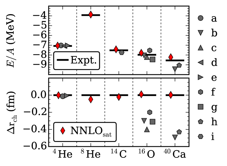
Figure 26: Ground-state energy (negative of binding energy) per nucleon (top), and residuals (differences between computed and experimental values) of charge radii (bottom) for selected nuclei computed with a variety of chiral potentials (labeled a—i and $\text{NNLO}_{\text{sat}}$). Figure and description taken from Ekström et al. (2015). Courtesy of A. Ekström.

The role of the regulator has also been under increasing scrutiny in ab initio calculations. A powerful tool for many-body calculations is quantum Monte Carlo (QMC), which pioneered the modern solution of many-nucleon systems but is best suited for local potentials. In Chiral EFT, it favors local interactions and regulators. Antisymmetrization among nucleons can be used to eliminate some non-local contact interactions Gezerlis et al. (2013, 2014); Lynn et al. (2014); Piarulli et al. (2016); Logoteta et al. (2016), enabling various new calculations. For example, the effects of the $\mathcal{O}(Q^{2}/M_{\text{QCD}}^{2})$ potential in neutron matter have been studied Gezerlis et al. (2013, 2014); Tews et al. (2016); Lynn et al. (2016). Because of antisymmetrization, different spin-isospin forms of the $3N$ contact interaction can be written, which are all equivalent and consistent with zero within the EFT truncation error for $\Lambda\stackrel{{\scriptstyle>}}{{{}_{\sim}}}M_{\text{QCD}}$. In contrast, the limitation to $\Lambda\stackrel{{\scriptstyle<}}{{{}_{\sim}}}M_{\text{QCD}}$ leads to relatively large regulator artifacts above saturation density Lynn et al. (2016). This indicated that a lack of RG invariance, besides destroying model-independence, also has undesirable phenomenological consequences.

IV.4.2 Renormalization of singular potentials

The regulator dependence of Weinberg’s prescription has been understood for a long time. Historically the first observation was that the potential (72) can be solved semi-analytically in the ${}^{1}S_{0}$ channel: if $p$ ($\mbox{\boldmath$p$}^{\prime}$) denotes the relative incoming (outgoing) momentum in the center-of-mass frame and $k^{2}/m_{N}$ the energy, the LO amplitude can be written Kaplan et al. (1996); Gegelia (1999b); Eiras and Soto (2003); Long and Yang (2012b)

$$T^{(0)}(\mbox{\boldmath$p$}^{\prime},\mbox{\boldmath$p$};k)=T_{\mathrm{Y}}(\mbox{\boldmath$p$}^{\prime},\mbox{\boldmath$p$};k)+\frac{\chi(\mbox{\boldmath$p$}^{\prime};k)\chi(\mbox{\boldmath$p$};k)}{C_{0\mathrm{s}}^{-1}(\Lambda)-I(\Lambda;k)}\,,$$ (75)

where $T_{\mathrm{Y}}$ is the amplitude for a pure Yukawa potential and

$$\chi(\mbox{\boldmath$p$};k) =1+m_{N}\int\frac{\mathrm{d}^{3}l}{(2\pi)^{3}}\frac{T_{\mathrm{Y}}(\mbox{\boldmath$l$},\mbox{\boldmath$p$};k)}{k^{2}-\mbox{\boldmath$l$}^{2}+\mathrm{i}\epsilon}\,,$$ (76)

$$I(\Lambda;k) =m_{N}\int\frac{\mathrm{d}^{3}l}{(2\pi)^{3}}\frac{\chi^{{2}}(\mbox{\boldmath$l$};k)}{k^{2}-\mbox{\boldmath$l$}^{2}+\mathrm{i}\epsilon}{\,,}$$ (77)

where we keep the regularization implicit. When $T_{\mathrm{Y}}=0$, $I(\Lambda;k)$ reduces to the $I_{0}(\Lambda;k)$ of Eq. (22), and Eq. (75) to Eq. (14). While $T_{\mathrm{Y}}$ and $\chi$ have no non-negative-power dependence on $\Lambda$, $I(\Lambda;k)$ has two types of inadmissible cutoff dependence: $\propto\Lambda$ and $\propto(m_{\pi}^{2}/M_{N\!N})\ln(\Lambda/M_{N\!N})$. The former is the same cutoff dependence one sees in Pionless EFT (Sec. II), and can be absorbed in $C_{0\mathrm{s}}$. The latter cutoff dependence, which appears despite the fact that the Yukawa interaction is regular by itself and is formally the same as the logarithmic divergence generated by the Coulomb interaction (see Sec. II.2.7), comes from the interference between contact interaction and OPE. It does not appear in other singlet channels Eiras and Soto (2003); Nogga et al. (2005), but it cannot be absorbed in $C_{0\mathrm{s}}$, which is the LEC of a chiral-invariant interaction and thus is not linear in $m_{\pi}^{2}$. Instead, one has to modify the LO potential (72) by Kaplan et al. (1996)

$$C_{0\mathrm{s}}\to C_{0\mathrm{s}}+m_{\pi}^{2}D_{2\mathrm{s}}=\mathcal{O}\left(\frac{4\pi}{m_{N}M_{N\!N}}\right)\,.$$ (78)

Even though NDA estimates $D_{2\mathrm{s}}=\mathcal{O}(C_{0\mathrm{s}}/M_{\text{QCD}}^{2})$, renormalization requires $D_{2\mathrm{s}}=\mathcal{O}(C_{0\mathrm{s}}/M_{\text{lo}}^{2})$. Because of the different transformation properties under chiral symmetry, the two operators with LECS $C_{0\mathrm{s}}$ and $D_{2\mathrm{s}}$ differ in their pion interactions, see Eq. (69c). Of course, one cannot see this problem numerically in the $2N$ system unless one varies $m_{\pi}$, which is not done in most nuclear work, and even then the divergence is only logarithmic. The additional pion interactions from $D_{2\mathrm{s}}$ should have effects on other processes, such as pion-nucleus scattering, but only when there is a significant contribution from the ${}^{1}S_{0}$ $2N$ partial wave. Regardless of its phenomenological (ir)relevance, this is the simplest example where the renormalization of observables in Chiral EFT is not guaranteed by NDA. This result has been confirmed in many other studies Beane et al. (2002); Pavón Valderrama and Ruiz Arriola (2004, 2006a).

A similar but more dramatic renormalization effect concerns the momentum dependence of OPE. The tensor potential is singular, behaving at short distances as $-\alpha/r^{n}$ with $n=3$ and, in some channels, $\alpha>0$. It is well known Frank et al. (1971) that such potentials need to be treated carefully because both solutions of the radial Schrödinger equation are irregular at $r=0$. For two particles of reduced mass $\mu$, the zero-energy $S$-wave radial wavefunction behaves at short distances as

$$\psi(r)=r^{n/4-1}\cos\left(\frac{\sqrt{2\mu\alpha}\,r^{1-n/2}}{n/2-1}+\phi_{n}\right)+{\cdots}\,,$$ (79)

where $\phi_{n}$ is a phase related to the scattering length and, more generally, the phase shifts. In EFT, the phase is determined by a contact interaction, the LEC of which displays an oscillatory dependence on the cutoff Beane et al. (2001a); Bawin and Coon (2003); Braaten and Phillips (2004); Alberg et al. (2005); Hammer and Swingle (2006); Bouaziz and Bawin (2014); Odell et al. (2019), characteristic of a limit cycle or more complicated attractor. For RG analyses and reviews of limit cycles, see Barford and Birse (2003, 2005); Pavón Valderrama and Ruiz Arriola (2008), and Hammer and Platter (2011); Bulycheva and Gorsky (2014), respectively. Without the contact interaction, the increasing attraction of the singular potential leads to the repeated appearance of low-energy bound states as the momentum cutoff increases. With the contact interaction, not only the two-, but also the three-body system is renormalized properly Odell et al. (2019), at least for $n=3$.

The argument can be generalized to the tensor force Beane et al. (2002); Birse (2006), which is attractive in some uncoupled channels and has one attractive eigenvalue in coupled channels. In ${}^{3}S_{1}$-${}^{3}D_{1}$, the $C_{0\mathrm{t}}$ interaction in Eq. (72) is sufficient to absorb the cutoff dependence and fix the low-energy phase shifts Frederico et al. (1999); Beane et al. (2002); Pavón Valderrama and Ruiz Arriola (2005, 2006a); Yang et al. (2008), as suggested by NDA. However, in higher partial waves the effects of $C_{0\mathrm{t}}$ are cutoff artifacts that disappear at large cutoffs. As the cutoff increases, bound states accrue in the higher partial waves where the tensor OPE is attractive (${}^{3}P_{0}$, ${}^{3}P_{2}$-${}^{3}F_{2}$, ${}^{3}D_{2}$, ${}^{3}D_{3}$-${}^{3}G_{3}$, etc.), leading to wild variation in the corresponding low-energy phase shifts Nogga et al. (2005); Pavón Valderrama and Ruiz Arriola (2006b). This problem can be cured Nogga et al. (2005) by a short-range interaction in each such wave, e.g., including a term $C^{\prime}_{2\mathrm{t}}(\mathbf{p}^{\prime}\cdot\mathbf{p})P_{\mathrm{t}}$ in Eq. (72). As primordial counterterm, $C^{\prime}_{2\mathrm{t}}=\mathcal{O}(C_{0\mathrm{s}}/M_{\text{QCD}}^{2})$ appears only at $\mathcal{O}(Q^{2}/M_{\text{QCD}}^{2})$, and similarly for the counterterms in other attractive, singular waves. The absence in Weinberg’s prescription of the appropriate counterterms explains the need for a “physical cutoff” $\Lambda_{\text{phys}}\stackrel{{\scriptstyle<}}{{{}_{\sim}}}1\leavevmode\nobreak\ \mathrm{GeV}$, where ${}^{3}P_{0}$ would develop a bound state Nogga et al. (2005). In other waves, bound states cross threshold at higher cutoffs. In triplet waves where OPE is repulsive there is no need for such counterterms at LO Eiras and Soto (2003); Nogga et al. (2005).

Renormalization problems have been reported Pavón Valderrama and Ruiz Arriola (2006a, b); Entem et al. (2008); Yang et al. (2009a, b); Zeoli et al. (2013) within Weinberg’s prescription also for higher-order potentials, which are increasingly singular and attractive in other waves as well. In contrast, a perturbative treatment of more-singular corrections to singular potentials can be properly renormalized Long and van Kolck (2008) with counterterms containing more derivatives, as expected from NDA. Renormalization of chiral potentials seems to demand that at least some parts of the potential be treated in perturbation theory, just like in Pionless EFT.

IV.4.3 Connection with Pionless EFT

Experience with Pionless EFT Bedaque and van Kolck (1998); van Kolck (1997); Kaplan et al. (1998a, b); Bedaque et al. (1998); van Kolck (1999b) shows that the factors associated with reducible loops are [eq:ConnectionPionlessPC] potential &∼4πm_N^-1 M_lo^-1(Q M_QCD^-1)^μ  ,
nucleon prop. ∼m_N Q^-2  ,
reducible loop int. ∼(4πm_N)^-1 Q^5  , where the factor of $(4\pi)^{{-}1}$ is typical of integrals involving Schrödinger propagators. One iteration of the order-$\mu$ potential adds a reducible loop and two nucleon propagators, or $(Q/M_{\text{lo}})(Q/M_{\text{QCD}})^{\mu}$. This is an IR enhancement of $m_{N}/(4\pi Q)$ over the factor that arises from Eqs. (IV.3.1) and (IV.3.1). As a consequence, the perturbative series in the LO potential ($\mu=0$) fails to converge for $Q\sim M_{\text{lo}}$, while subleading potentials ($\mu\geq 1$) should be amenable to perturbation theory.

The LO chiral potential (72) has the form (IV.4.3) if $M_{N\!N}=\mathcal{O}(M_{\text{lo}})$. Since bound states indicate a breakdown of perturbation theory, one expects binding energies per nucleon

$$\frac{B_{A}}{A}\sim\frac{M_{N\!N}^{2}}{M_{\text{QCD}}}\sim\frac{f_{\pi}}{4\pi}\sim 10\leavevmode\nobreak\ \mathrm{MeV}\,,$$ (80)

which is in the right ballpark for heavy nuclei. Thus chiral symmetry together with this IR enhancement provides a natural explanation Bedaque and van Kolck (2002) for the shallowness of nuclei compared to $M_{\text{QCD}}$, $B_{A}/A\ll M_{\text{QCD}}$, long considered a mystery.

The factor of $4\pi$ in the IR enhancement was not recognized before Pionless EFT was developed, but it has implications for the natural size of few-body forces. Connecting an $aN$ potential to another nucleon to make it an $(a+1)N$ potential without changing $L$ or $\Delta$ involves an additional factor $4\pi m_{N}^{-1}M_{\text{lo}}^{-2}$ from the extra $2N$ interaction and the extra nucleon propagator inside the $aN$ potential. At the same time, it adds a reducible loop and one nucleon propagator at the amplitude level, resulting in an overall suppression by $Q/m_{N}$. For $m_{N}=\mathcal{O}(M_{\text{QCD}})$—as dictated by NDA for $A=1$, where it works well—this is the $n=1$ suppression of Friar (1997). In contrast, missing the $4\pi$ in the IR enhancement would require $Q/m_{N}\sim Q^{2}/M_{\text{QCD}}^{2}$, as found in Sec. IV.3.2 for $n=2$ Weinberg (1991); Ordóñez and van Kolck (1992); Weinberg (1992); van Kolck (1993). Thus, counting factors of $4\pi$ in reducible loops leads to Friar’s power counting, which, however, has not been widely tested so far.

IV.4.4 Perturbative pions

A radical solution to the renormalization problems of Weinberg’s prescription was proposed by Kaplan et al. (1998a, b): assume the contact interactions carry a low-energy scale characteristic of the binding momenta of light nuclei, $M_{\text{lo}}\ll M_{N\!N}$, and treat $M_{N\!N}$ as a high-energy scale. Pion exchange in nuclear amplitudes appears in two expansions:

1. The expansion in $Q/(4\pi f_{\pi})$ of the nuclear potential, which, as discussed in Sec. IV.3.2, is similar to the ChPT expansion for $A\leq 1$.

2. An expansion in $Q/M_{N\!N}$ in the solution of the dynamical equation, which is similar to the Pionless EFT expansion for $A\geq 2$.

Thus, if $Q\sim m_{\pi}\ll M_{N\!N}\stackrel{{\scriptstyle<}}{{{}_{\sim}}}M_{\text{QCD}}$ one can treat all pion exchanges in perturbation theory. Numerically $M_{N\!N}$ could be larger than the NDA estimate $M_{N\!N}\sim f_{\pi}$.

This version of Chiral EFT closely resembles Pionless EFT (Sec. II), with similar $M_{\text{lo}}$ scaling of the LECs but different values, and additional pion exchanges. The range of validity of the EFT is enlarged, at least near the chiral limit where integrating out pions becomes a very restrictive condition. At LO the two EFTs are formally the same, so the corresponding results from Pionless EFT carry over (there are two non-derivative $2N$ contact interactions and one non-derivative three-nucleon force), but $m_{\pi}$ is now counted as $M_{\text{lo}}$ together with the $2N$ binding momenta.

At relative $\mathcal{O}(Q/M_{N\!N})$, however, there are not only two-derivative two-nucleon contact terms ($\propto Q^{2}$) but also OPE, which provides a shape function that goes beyond the first two terms in the effective-range expansion. In perturbation theory, the $m_{\pi}^{2}\ln\Lambda$ cutoff dependence in the ${}^{1}S_{0}$ channel (Sec. IV.4.2) comes from a diagram where OPE appears in-between two LO interactions. The corresponding chiral-symmetry breaking counterterm ($\propto m_{\pi}^{2}$) must be NLO as well. Both $Q^{2}$ and $m_{\pi}^{2}$ corrections appear at the same order, as in ChPT, but they are suppressed by only one power of $Q/M_{N\!N}$. The two-nucleon amplitude is well reproduced Kaplan et al. (1998a, b); Soto and Tarrus (2008). (For the renormalization issues associated with a resummation of effective-range effects with and without dibaryon fields, see Ando and Hyun (2012) and Nieves (2003), respectively.) There is only one calculation of the effects of perturbative OPE in the three-nucleon system—quartet $nd$ scattering below and above break-up Bedaque and Grießhammer (2000)—and it gives results very similar to those from Pionless EFT (Sec. II.3.3).

N²LO Fleming et al. (2000a); Cohen and Hansen (1999b); Fleming et al. (2000b); Soto and Tarrus (2010), i.e., relative $\mathcal{O}(Q^{2}/M_{N\!N}^{2})$ is a crucial test of this expansion, since it is the first manifestation of iterated OPE. It was demonstrated Cohen and Hansen (1999b); Fleming et al. (2000b) that, while the expansion works well at small momenta, in the low, spin-triplet partial waves where the OPE tensor force is attractive, it fails for momenta $Q\sim 100\leavevmode\nobreak\ \mathrm{MeV}$. Fleming et al. (2000b) employed dimensional regularization with a power-divergence subtraction (PDS) Kaplan et al. (1998a, b) designed to facilitate power counting, but of course other regularization/subtraction schemes give equivalent results Cohen and Hansen (1998); Mehen and Stewart (1999a, b). (For an RG discussion, see Harada et al. (2011).) A calculation employing a procedure similar to Pauli-Villars regularization gave better results Beane et al. (2009) in channels with LECs, but not in the spin-triplet channels lacking LECs at that order. These signs of the breakdown of perturbative pions are consistent with an expansion in $Q/M_{N\!N}$ where $M_{N\!N}\sim f_{\pi}$ as indicated by NDA.

There has also been criticism of the perturbative-pion expansion based on the poor convergence of threshold observables Cohen and Hansen (1999a, c). This suggests that the expansion in $m_{\pi}/M_{N\!N}$ is not great for the real world, again pointing to the low value of $M_{N\!N}$. However, it is the reorganization of interactions in Pionless EFT that is optimized for momenta $Q\ll m_{\pi}$, where the ERE holds. The effectiveness of a power counting in Chiral EFT should be judged from the convergence of observables at $Q\sim m_{\pi}$. At such momenta, for example, the scattering length contribution is small, and one might start from the unitary limit instead Soto and Tarrus (2008, 2010), as discussed in Sec. II.4. In the ${}^{1}S_{0}$ channel, the perturbative-pion expansion does converge Beane et al. (2002) despite claims to the contrary based on an NLO calculation Gegelia (1998a). The slow convergence can be attributed to the short-range interactions. For analyses of perturbative pions in the better-controlled context of toy models, see Steele and Furnstahl (1999); Rupak and Shoresh (1999); Kaplan and Steele (1999).

In the real world, this version of Chiral EFT does not seem to work much beyond the regime of validity of Pionless EFT. Because the latter is simpler and holds for larger pion masses, it has been preferred in most low-energy applications. However, Chiral EFT retains the constraints of chiral symmetry that are lost in Pionless EFT; when such constraints are useful, Chiral EFT with perturbative pions can be deployed. Moreover, at smaller pion masses Chiral EFT with perturbative pions is expected to have a considerably larger range of applicability than Pionless EFT.

IV.4.5 Partly perturbative pions

For a couple of years the choice facing the field was between a power counting that lacks counterterms in the sense discussed in Sec. IV.4.2 (i.e., ensuring that all divergences at a given order can be absorbed) but worked well phenomenologically (Sec. IV.4.1), and another one that has all counterterms but failed to converge even at relatively small energies (Sec. IV.4.4). A way out was suggested by Nogga et al. (2005) and carried out by Valderrama (2011); Pavón Valderrama (2011); Long and Yang (2011, 2012a, 2012b). Perhaps not surprising in hindsight, this solution is a middle ground between Weinberg’s prescription and fully perturbative pions. It is based on two observations:

1. Pions are perturbative in sufficiently high two-nucleon partial waves. For an orbital angular momentum $l>l_{\text{cr}}$, where $l_{\text{cr}}(l_{\text{cr}}+1)\sim M_{\text{hi}}/M_{N\!N}$, the centrifugal barrier dominates over OPE at all distances $r\stackrel{{\scriptstyle>}}{{{}_{\sim}}}1/M_{\text{hi}}$ relevant when $Q\lesssim M_{\text{hi}}$. In these waves OPE should be perturbative for the external momenta where Chiral EFT holds Nogga et al. (2005). In other words, OPE in the radial Schrödinger equation is an expansion in $Q/M_{N\!N}^{(l)}$, where $M_{N\!N}^{(0)}=M_{N\!N}$ but $M_{N\!N}^{(l)}$ increases with $l$. For $l\leq l_{\text{cr}}$, OPE is nonperturbative. In these waves, and in these waves only, OPE needs to be iterated at LO, as observed by Fleming et al. (2000b). The LECs needed for renormalization (Sec. IV.4.2) should, of course, be iterated as well. All subleading interactions are to be treated in distorted-wave perturbation theory for $l\leq l_{\text{cr}}$, and in ordinary perturbation theory for $l>l_{\text{cr}}$.

2. Multiple pion exchange, being suppressed by powers of $Q/(4\pi f_{\pi})$, should be small after renormalization, and thus amenable to perturbation theory in all waves. It is more singular than OPE, but can be renormalized perturbatively with a finite number of LECs Long and van Kolck (2008).

Since the OPE tensor force survives in the chiral limit, for $m_{\pi}\stackrel{{\scriptstyle<}}{{{}_{\sim}}}M_{N\!N}$ one can perform an additional expansion around the chiral limit Beane et al. (2002), but, as discussed in Sec. IV.4.4, this expansion is not likely to be useful much beyond the physical pion mass.

For $M_{\text{hi}}>M_{N\!N}$, i.e., $M_{N\!N}$ counted as a low-energy scale, one expects $l_{\text{cr}}\geq 1$. Of course, other dimensionless factors stemming from spin and isospin make the transition from nonperturbative to perturbative OPE somewhat fuzzy, which however does not mean that such a transition does not exist. Early studies of perturbative pions with and without Deltas Kaiser et al. (1997); Ballot et al. (1998); Kaiser et al. (1998), which did not discriminate between iterated pion exchange and multiple pion exchange in the potential, indicated that pion exchange might be perturbative for $l\stackrel{{\scriptstyle>}}{{{}_{\sim}}}3$. This interpretation is also consistent with subsequent investigations of peripheral waves with chiral potentials up to $\mathcal{O}(Q^{6}/M_{\text{QCD}}^{6})$ Entem and Machleidt (2002); Epelbaum et al. (2004a); Krebs et al. (2007); Entem et al. (2015b, a). Qualitatively, this result has been confirmed for OPE Nogga et al. (2005). A semi-analytical estimate Birse (2006) of the momenta where the tensor part of OPE needs to be treated nonperturbatively in the lower triplet waves is given in Table 2. Some evidence thus points to $l_{\text{cr}}\approx 3$. More detailed, recent analyses suggest, however, that pions are perturbative up to a relatively high scale in all waves other than ${}^{3}S_{1}$-${}^{3}D_{1}$ and ${}^{3}P_{0}$ Wu and Long (2019); Kaplan (2019).

Channel	$p_{\text{cr}}$/MeV	Channel	$p_{\text{cr}}$/MeV	Channel	$p_{\text{cr}}$/MeV
${}^{3}S_{1}$-${}^{3}D_{1}$	66	${}^{3}P_{0}$	182	${}^{3}P_{1}$	365
${}^{3}P_{2}$-${}^{3}F_{2}$	470	${}^{3}D_{2}$	403	${}^{3}D_{3}$-${}^{3}G_{3}$	382
${}^{3}F_{3}$	2860	${}^{3}F_{4}$-${}^{3}H_{4}$	2330	${}^{3}G_{4}$	1870

Table 2: Estimate of the critical values $p_{\text{cr}}$ of the relative momentum in the lowest two-nucleon triplet channels above which the OPE tensor force cannot be treated perturbatively Birse (2006).

In the low $2N$ waves where $l\leq l_{\text{cr}}$ and $M_{N\!N}^{(l)}\approx M_{N\!N}$, the situation at LO is similar to Weinberg’s prescription, except that more short-range interactions are needed for renormalization Nogga et al. (2005) than implied by NDA. For example, in the ${}^{1}S_{0}$ channel OPE at LO solves the problem of the slow convergence of perturbative pions Beane et al. (2002) at the cost of the additional $D_{2\rm s}$ LEC in Eq. (78). The residual $1/\Lambda$ dependence then means Long and Yang (2012b) that a correction appears at $\mathcal{O}(Q/M_{\text{QCD}})$ from the two-derivative contact interaction responsible for the short-range contribution to the effective range, similarly to Pionless EFT (Sec. II.2.3). At higher orders in the lower partial waves, multiple-pion exchanges appear and require at $\mathcal{O}(Q^{\mu}/M_{\text{QCD}}^{\mu})$ LECs with up to $\mu$ derivatives more than the LECs appearing at LO Long and van Kolck (2008).

This approach was confronted with empirical phase shifts for the lower $2N$ partial waves by Nogga et al. (2005); Epelbaum and Meißner (2013); Valderrama (2011); Pavón Valderrama (2011); Long and Yang (2011, 2012a, 2012b); Yang (2016). The results of Long and Yang (2012a) are included in Fig. 7, whereas Fig. 27 shows the ${}^{3}P_{0}$ results of Pavón Valderrama (2011) as a further example. While in both cases $\mathcal{O}(Q^{2}/M_{\text{QCD}}^{2})$ improves on $\mathcal{O}(1)$, $\mathcal{O}(Q^{3}/M_{\text{QCD}}^{3})$ goes in the wrong direction—perhaps an indication that a better description of the pion-nucleon subamplitude with an explicit Delta isobar is needed.

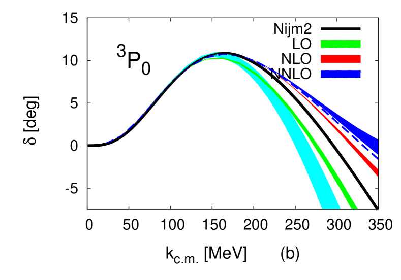
Figure 27: The $N\!N$ ${}^{3}P_{0}$ phase shift $\delta$ as a function of the center-of-mass momentum $k_{c.m.}$ at different chiral orders: ${\mathcal{O}}(1)$ (green), ${\mathcal{O}}(Q^{2}/M_{\text{QCD}}^{2})$ (red), and ${\mathcal{O}}(Q^{3}/M_{\text{QCD}}^{3})$ (blue), according to Pavón Valderrama (2011). Bands represent the variation of a coordinate-space cutoff in the range 0.6–0.9 fm, with the dashed line showing the ${\mathcal{O}}(Q^{3}/M_{\text{QCD}}^{3})$ results with a 0.3 fm cutoff. The cyan band shows the ${\mathcal{O}}(Q^{3}/M_{\text{QCD}}^{3})$ potential in Weinberg’s prescription with the regularization procedure of Epelbaum et al. (2004b), where the momentum-space cutoff in pion loops (Lippmann-Schwinger equation) is varied between 500 and 700 (450 and 650) MeV. The solid black line is the Nijmegen phase-shift analysis Stoks et al. (1993). Figure from Pavón Valderrama (2011). Courtesy of M. Pavón Valderrama.

Little is known quantitatively about partly perturbative pions beyond the two-nucleon system. The three-nucleon system is renormalized properly without a three-nucleon force at LO Nogga et al. (2005); Song et al. (2017b) and, without explicit Deltas, also at NLO Song et al. (2017b). The truncation in $l$ needed at LO is reminiscent of the truncation in total two-nucleon angular momentum typically invoked in solutions of the Faddeev and Faddeev-Yakubovski equations for three- and four-nucleon systems with phenomenological potentials. However, to go to higher orders the $l$ dependence of $M_{N\!N}^{(l)}$ must be quantified. So far, this has been done only in singlet waves Pavón Valderrama et al. (2017).

At LO, symmetric nuclear matter was found to saturate, but with significant underbinding, in a cutoff-converged Brueckner pair approximation Machleidt et al. (2010). This is in contrast to Weinberg’s prescription, where Deltaless Sammarruca et al. (2018) or Deltaful Ekström et al. (2018) potentials of $\mathcal{O}(1)$ and $\mathcal{O}(Q^{2}/M_{\text{QCD}}^{2})$ do not saturate within the EFT domain. The fact that higher-order potentials with this prescription do saturate Ekström et al. (2018); Drischler et al. (2019); Sammarruca et al. (2018) suggests that, if nuclear matter is within the regime of Chiral EFT, the LO potential requires more interactions than prescribed by NDA.

Although they differ in detail from the field-theoretical renormalization outlined above, RG analyses of the Schrödinger equation Birse (2006, 2011); Valderrama (2016) support the conclusion that counterterms in two-nucleon attractive singular waves appear at lower order than expected on the basis of NDA. The case is further strengthened by removing the effect of OPE and (perturbative) TPE from empirical two-nucleon phase shifts Birse (2007); Ipson et al. (2011). The Schrödinger RG analysis also predicts the enhancement of some three-body forces Birse (2011).

IV.4.6 Other approaches

The renormalization of Chiral EFT described in the previous section was criticized by Epelbaum et al. (2018), who provided examples where the nonperturbatively renormalized amplitude exhibits positive powers of the cutoff $\Lambda$ when expanded in Planck’s constant $\hbar$. Since no observable considered in that work is affected, however, the significance of this claim for an EFT is unclear. Moreover, Valderrama (2019) argued that these powers of $\Lambda$ can be eliminated by changing the $\Lambda^{-1}$ running of the LECs Valderrama (2016). (See also the response by Epelbaum et al. (2019).)

An alternative approach to the renormalization woes of Weinberg’s prescription was articulated by Epelbaum et al. (2018), building on earlier work Gegelia (1998b, 1999a, a, 1999b); Gegelia and Japaridze (2001); Gegelia and Scherer (2006); Epelbaum and Gegelia (2009). It consists of renormalizing the perturbative series and subsequently resumming the renormalized contributions, that is, it includes at each order the infinite number of LECs needed to eliminate the cutoff dependence of all diagrams to be resummed. These LECs exist because an EFT contains all interactions allowed by symmetry, but even without pions they are difficult or impossible to write down explicitly. In a stark departure from naturalness, only the LECs prescribed by NDA are assumed to contribute finite parameters, which amounts to an infinite number of fine tunings. The resummation of an infinite number of derivative interactions introduces an intrinsic nonlocality in all channels at every order—not only LO in, say, the $N\!N$ ${}^{1}S_{0}$ Beane and Savage (2001); Sánchez Sánchez et al. (2018) or the $N\alpha$ ${}^{2}P_{3/2}$ Bertulani et al. (2002) channels, where there are shallow poles.

In this approach, there are no constraints on the EFT from renormalization, for example no Wigner bound on the effective range (Wigner (1955); see Sec. II.2.3) when $C_{2}$ or higher-order interactions are resummed Gegelia (1998b) and no explanation Epelbaum et al. (2017b, 2019) for the emergence of a single, independent three-body scale in the three-body system at LO, which determines the position of the Efimov tower of states (Efimov (1970b); see Sec. II.3.2). Thus, the justification for power counting from the combination of renormalization and naturalness, which in the perturbative context gives NDA Manohar and Georgi (1984); Georgi and Randall (1986), is absent. NDA becomes an ad hoc rule. It does not, e.g., reproduce the established scaling of range corrections in amplitudes resulting from short-range potentials, which is represented in Pionless EFT through Eq. (18).

So far this approach has been implemented only in the ${}^{1}S_{0}$ channel, where significant dependence on the choice of (low-energy) subtraction points is seen Gegelia (1999a, 1998a, b); Gegelia and Japaridze (2001). On the basis of a toy model, Epelbaum et al. (2017a) conclude that Weinberg’s prescription is satisfactory as long as the renormalization scale $\mu=\mathcal{O}(M_{\text{hi}})$. Chiral EFT’s overlapping integrals in other channels prevent the explicit resummation of “renormalized diagrams” and it is not known whether this procedure, if it can be carried out at all, reproduces the nonperturbative solution of the Lippmann-Schwinger equation. Further discussion of renormalization from the perspective of subtraction schemes can be found in Timoteo et al. (2011); Szpigel and Timoteo (2012); Batista et al. (2017).

Gegelia and Japaridze (2001) offer the solution that the cutoff should not be varied significantly around the breakdown scale in Chiral EFT. In the absence of renormalization, non-negative powers of the cutoff should appear in the truncated amplitude given by Eq. (6) as corrections of $\mathcal{O}(Q^{\mathcal{V}+1-i}\Lambda^{i}/(M_{\text{hi}}^{\mathcal{V}+1-j}M_{\text{lo}}^{j}))$ with nonnegative integers $i,j$. If $j=0$ the corrections should be small for $\Lambda\ll M_{\text{hi}}$ Gegelia and Scherer (2006), but $j>0$ arises when the LO potential, which does not involve $M_{\text{hi}}$, is singular.

An attempt to mitigate cutoff artifacts was made by Djukanovic et al. (2007), Epelbaum and Gegelia (2012), and Epelbaum et al. (2014, 2015a) with the most recent formulations developed by Behrendt et al. (2016) and Baru et al. (2019b). A nucleon propagator with faster large-momentum fall-off is constructed by demanding that states satisfy a relativistic (Lorentz-invariant) normalization condition, while overall the treatment is still nonrelativistic. This softer UV behavior helps to obtain LO amplitudes with well-defined large-cutoff limits. While Behrendt et al. (2016) state that higher orders should be treated in perturbation theory if this feature is to be maintained beyond LO, from a practical point of view they still advocate a nonperturbative treatment (where the cutoff is then limited again to a finite range, argued to be larger than what is typically used with standard Weinberg counting). Moreover, Behrendt et al. (2016) find that with their approach a ${}^{3}P_{0}$ LEC has to be promoted compared to NDA, as in the purely nonrelativistic context Nogga et al. (2005). There is, nevertheless, growing interest in the development of a covariant version of Chiral EFT, which could perhaps be used as input to relativistic formulations of nuclear physics Petschauer and Kaiser (2013); Ren et al. (2018, 2017).

IV.5 Pion and electroweak reactions

One of the great advantages of a quantum-field-theoretical foundation of nuclear physics is that not only many-body forces can be constructed consistently with two-body forces, but also many-body currents can be derived consistently with inter-nucleon interactions. This virtue was realized early on Rho (1991); Weinberg (1991), and some of the pioneering papers on reactions have been dedicated to electroweak currents Park et al. (1993, 1996b); Phillips and Cohen (2000), neutron radiative capture on the proton Park et al. (1995, 1998a), proton-proton fusion Park et al. (1998b), Compton scattering on the deuteron Beane et al. (1999), pion photo- Beane et al. (1995, 1997) and electro- Bernard et al. (2000) production off the deuteron, pion photoproduction off the trinucleon Lenkewitz et al. (2011, 2013), pion scattering on the deuteron Beane et al. (1998a) and helion Liebig et al. (2011), as well as pion production in $2N$ collisions Park et al. (1996a); Cohen et al. (1996); van Kolck et al. (1996b); Sato et al. (1997). The goal is not only to supply information to other areas of physics where these reactions play a role, but also to extract nucleon properties (in particular for the neutron, for which good targets do not exist) to infer properties of the QCD dynamics.

The early work, reviewed by van Kolck (1999a) and Bedaque and van Kolck (2002), was based on Weinberg’s prescription, where, in addition to the potential, also the kernel of the reaction process is expanded according to NDA. For probes with energies $E\sim Q\sim m_{\pi}$, the kernel is defined as the subdiagrams to which the external probes are attached, energies are comparable to momenta, and nucleons are approximately static. Like the potential, kernels can be multiply connected, and power counting is similar to Eqs. (71) and (IV.3.1). For any kernel, a figure like Fig. 25 can be drawn. However, some subtleties need to be taken into account when probes have other typical energy or momentum:

• $E\sim M_{N\!N}^{2}/M_{\text{QCD}}$ (e.g. Compton scattering): a resummation is needed between kernels because infrared enhancements appear in intermediate states, where nucleons are not static Beane et al. (1999).

• $Q\sim\sqrt{m_{\pi}m_{N}}$ (e.g. pion production): intermediate states containing only nucleons can be part of the kernel, but these nucleons are not static Cohen et al. (1996).

The full amplitude is given by the matrix element of the kernel with wavefunctions obtained from the potential. In Weinberg’s prescription, these wavefunctions are exact solutions of a truncated potential. Much of the work predating phenomenologically successful chiral potentials employed a “hybrid” approach where the kernel was calculated in Chiral EFT but wavefunctions from “realistic” phenomenological potentials were used. Emphasis has since been shifting towards increased consistency between wavefunctions and kernels. Reactions are an area of renewed interest in Chiral EFT, in consonance with the revival of development in the broader area of nuclear reactions, including ab initio approaches. Of particular recent interest have been electroweak currents, where earlier work was revisited and significantly improved upon—see the excellent reviews by Phillips (2016) and Riska and Schiavilla (2017). There has also been substantial work on reactions involving pions, particularly pion production in two-nucleon collisions, which has now been calculated up to three orders in the chiral expansion Baru et al. (2014).

The process that has been most thoroughly examined in Chiral EFT is Compton scattering (CS). It gives access to nucleon polarizabilities—response functions that carry much information about hadron dynamics. While proton polarizabilities can be extracted directly, neutron polarizabilities can only be probed in nuclear CS. Chiral EFT allows for a consistent treatment of both these cases, and at the same time enables a connection with lattice QCD through variation in the pion mass. Recent work has capitalized on all advances in EFT and provides an analysis of CS that is a model for future work on nuclear reactions. At the one-nucleon level, CS was calculated in ChPT with an explicit Delta isobar McGovern et al. (2013), including the resummation Pascalutsa and Phillips (2003) needed to go through the Delta peak. At the nuclear level, the kernel was calculated consistent with Weinberg’s prescription Grießhammer et al. (2012a). Proton McGovern et al. (2013) and deuteron Myers et al. (2014, 2015) data were fitted and polarizabilities were extracted, see Fig. 28. The average quark mass was then varied to produce predictions, with uncertainties determined via Bayesian techniques Furnstahl et al. (2015c, b); Wesolowski et al. (2016), for the polarizabilities at unphysical pion masses Grießhammer et al. (2016b), to which lattice QCD results can be compared. Analyses of this type for other processes should increasingly become standard in this field, allowing to bridge from QCD to nuclear reactions just as to nuclear structure.

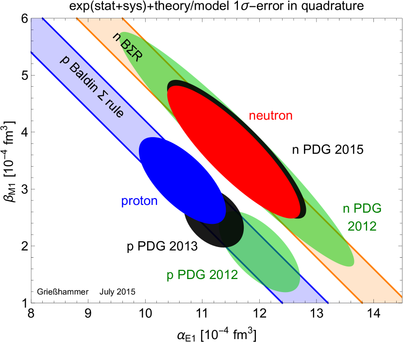
Figure 28: Nucleon electric ($\alpha_{{\rm E}1}$) and magnetic ($\beta_{{\rm M}1}$) polarizabilities extracted with Chiral EFT. Ellipses show the 1$\sigma$-error fits of McGovern et al. (2013) for proton (blue, on lower band) and neutron (red, on upper band), where statistic, systematic, and theory errors were added in quadrature. For comparison, Particle Data Group averages before (large, green ellipses) and after (small, black ellipses) these fits are also given. The bands are the constraints from the Baldin sum rule. Reprinted from Grießhammer et al. (2016a), with the permission of AIP Publishing.

The renormalization problems of Weinberg’s prescription demand scrutiny in the treatment of reactions as well. The emergence of a perturbative-pion formulation of Chiral EFT has led to a re-examination of many of the reactions that had been studied earlier with Weinberg’s prescription. With perturbative pions, not only the kernel but also the wavefunction is expanded in perturbation theory. For the deuteron—target of most, if not all, perturbative-pion studies—the analytical nature of the calculations makes it easier to establish proper renormalization. In most cases, the LO calculation is the same as in Pionless EFT (Secs. II.2.8 and II.3.8), and pion effects enter explicitly at subleading orders. For example, the charge, magnetic dipole and electric quadrupole form factors of the deuteron have been calculated to NLO by Kaplan et al. (1999b). Other reactions include neutron radiative capture on the proton Savage et al. (1999), deuteron Compton scattering and polarizability Chen et al. (1998b, a); Chen (1999), and neutrino-deuteron scattering Butler and Chen (2000). Generally, this approach has been successful for the low-energy properties of the deuteron, both in comparison with data and with nonperturbative-pion calculations.

IV.6 Outstanding issues and current trends

Within Weinberg’s prescription, work continues in pushing potential and kernels to higher orders, as well as developing better fitting strategies. Meanwhile, an RG-invariant formulation of Chiral EFT has not yet achieved the level of phenomenological impact of Weinberg’s prescription. Some of the outstanding questions are:

• What is the role of fine-tuning in Chiral EFT? The scattering length is particularly large in the ${}^{1}S_{0}$ two-nucleon channel, where short-range interactions show strong energy dependence Birse (2010). In particular, short-range contributions to the effective range are anomalously large, which has led to the suggestion that the two-derivative contact interaction ($C_{2\mathrm{s}}$ in Eq. (69c)) should be treated as LO Beane et al. (2002); Long (2013), following a similar proposal in Pionless EFT Beane and Savage (2001) (Sec. II.2.5) and Chiral EFT with perturbative pions Ando and Hyun (2012) (Sec. IV.4.4). Although an improved description is achieved, convergence deteriorates quickly with momentum, at least in a calculation without Deltas Long (2013). The role of the relatively low-energy zero of the amplitude remains to be fully investigated Lutz (2000); Sánchez Sánchez et al. (2018).

• What is the pion mass variation of nuclear amplitudes? To determine this variation, we need lattice data within the region of validity of Chiral EFT. While lattice QCD data exist at relatively large $m_{\pi}$, not all competing collaborations are in agreement. Moreover, differences exist within Chiral EFT depending on the approach used. Among the issues for extrapolations is the role of “radiation” pions, which are present only at relatively high order. Real pions can be produced in $2N$ collisions for momenta $Q\stackrel{{\scriptstyle>}}{{{}_{\sim}}}\sqrt{m_{\pi}m_{N}}$; at lower $Q$ the effects of the corresponding virtual pions are indistinguishable from the LECs Ordóñez et al. (1996); Epelbaum et al. (1998). These contributions have been investigated in the perturbative-pion context Mehen and Stewart (2000); Mondejar and Soto (2007); Soto and Tarrus (2012) where they give rise to powers of $m_{\pi}^{1/2}$.

• The NDA-based organization of pion-exchange contributions to the potential is not affected by the renormalization issues that plague Weinberg’s prescription, except for the possible enhancement factors of $4\pi$ in few-nucleon forces (Sec. IV.3.2). Once the $2N$ system has been properly renormalized, one must ask whether short-range many-body forces are immune to the enhancements seen in Pionless EFT (Sec. II.3.2). Most work on many-body forces in Chiral EFT takes Weinberg’s power counting for granted. Nogga et al. (2005) and Song et al. (2017b) have found no renormalization evidence for a $3N$ force in LO or $\mathcal{O}(Q/M_{\text{QCD}})$, but they obtain a triton binding energy which is only about half of the experimental value, perhaps because this is a very-low energy observables in the sense of being within the regime of Pionless EFT. Kievsky et al. (2017) argue from continuity with Pionless EFT that the $H_{0}$ three-body force in Eq. (69c) should be included at LO.

• The most important problem facing reaction theory in Chiral EFT echoes the renormalization woes of Weinberg’s prescription for nuclear structure. In order to maintain model independence, one must ensure that the average of the reaction kernel has a well-defined limit as the cutoff is increased. Only for electroweak reactions on the deuteron has this been investigated Pavón Valderrama and Phillips (2015); Phillips (2016), with the conclusion that enhancements over NDA appear there as well. The impact of this observation on previously studied reactions and future reaction theory remains to be investigated.

• To which extent can an RG-invariant formulation of Chiral EFT be incorporated in calculations of larger nuclei? Distorted-wave perturbation theory usually becomes very demanding in second order where the fully off-shell $A$-body propagation is needed in intermediate states. In Pionless EFT, this problem has been side-stepped by a reformulation in terms of the solution of further integral equations Vanasse (2013, 2017b). It is an open issue whether this or another method can be applied to the $A$-nucleon problem in Chiral EFT.

• Although not RG invariant, Weinberg’s prescription has several practical advantages because it is most closely related to previous phenomenological approaches. For example, it provides fits to data of comparable quality to “realistic” phenomenological potentials (Sec. IV.4.1), it explains some of the qualitative features of these potentials (Sec. IV.3.2), and it can be employed in already existing ab initio codes. Its successes beg the question, is it possible that a particular choice of regulator allows for a small-cutoff formulation of Chiral EFT that is equivalent to its RG-invariant form? It is conceivable that one can iterate subleading terms of the latter, as it is done in the former, within a limited range of cutoffs, just as iterating momentum-dependent contact interactions in Pionless EFT requires cutoff values $\Lambda\stackrel{{\scriptstyle<}}{{{}_{\sim}}}1/r_{0}$ (Wigner bound, Sec. II.2.3). If achieved, such an understanding of Weinberg’s prescription might justify current uses of Chiral EFT without requiring further development of ab initio methods. Furthermore, it will likely make it desirable to choose a regulator which optimizes convergence for the problem at hand, for example neutron matter Lynn et al. (2016). First steps in this direction were just made by Tews et al. (2018) and Pavón Valderrama (2019).

• Irrespective of other issues discussed above and throughout this section, it is a highly nontrivial task to determine the LECs of Chiral EFT—quite substantial in number at higher orders—from fitting calculated observables to data. One wants to do this in such a way that the EFT can fulfill its promises of providing systematic model independence and fully quantified uncertainties. For that, one should account for the truncation error of the EFT expansion directly as part of the fitting procedure, and propagate forward all this information to the final result of a calculation. Following the initial suggestion of Schindler and Phillips (2009), Bayesian methods have emerged in recent years Furnstahl et al. (2015c, b); Wesolowski et al. (2016); Melendez et al. (2017); Wesolowski et al. (2019) as an important tool to address the issue in a robust and comprehensive way.

V Broader applications

Many of the ideas originating in nuclear EFTs have found applications to other systems. Pionless EFT, while being clearly connected to QCD as a low-energy limit, is driven largely by the universal features that arise from the large $N\!N$ scattering lengths and the associated large sizes of light nuclei. As a consequence, the EFT for nuclear halo states discussed in Sec. III can be constructed as a generalization of Pionless EFT. But universality goes beyond nuclear physics: it is relevant to any system dominated by short-range interactions, when one is interested in distance scales much larger than the range of the interactions.

As one probes distances comparable to the interaction range, issues similar to the ones discussed in Chiral EFT emerge. For example, can the long-range part of the interaction be treated in perturbation theory? In other hadronic systems, the long-range interaction might still be one-pion exchange, and then Chiral EFT applies except that other heavy particles are substituted for nucleons.

In this section we briefly describe some of the systems where versions of Pionless and Chiral EFTs have found application. We start by discussing how these EFTs arise from QCD.

V.1 Connection with QCD

The inclusion of all possible interactions consistent with QCD symmetries ensures that nuclear EFTs capture the low-energy limit of QCD. This means that in principle one can follow a top-down approach and determine low-energy constants that appear in an EFT from a direct solution of the more general theory. While such solutions of QCD (in the highly nonperturbative low-energy regime) are elusive analytically, lattice calculations have made significant progress towards nuclear systems. Matching EFT to LQCD serves to extend the predictions of QCD in essentially two directions:

1. Larger distances: solution by ab initio methods of an EFT with parameters fixed by LQCD allows for predictions of properties of larger nuclei and their reactions, which are difficult to simulate directly from QCD.

2. Smaller pion masses: with the relative importance of chiral-symmetry-breaking interactions understood, Chiral EFT can be used as an extrapolation tool from larger quark—and thus pion—masses to the physical point.

Moreover, remnants of QCD’s color gauge symmetry can be traced down to nuclear EFTs. In particular, it is possible to consider the inverse number of colors, $1/N_{\rm c}$, as an expansion parameter to constrain nuclear forces. This has been studied, for example, by Kaplan and Manohar (1997); Phillips and Schat (2013); Phillips et al. (2015); Samart et al. (2016); Schindler et al. (2018).

V.1.1 Nuclear physics at large quark masses

The pion mass is a tunable parameter in LQCD. With calculations getting more expensive for lower pion masses, typically results are extracted for values of $m_{\pi}$ well above the physical point. Observables like hadron spectra can by now be described with amazing accuracy Kronfeld (2012), and results for hadronic properties have become available even at or below the physical pion masses. Direct QCD calculations of few-nucleon systems, however, still use relatively large pion masses (Beane et al. (2011) review the framework), and even then significant discrepancies exist among the outcomes from various groups. EFT calculations have used a subset of these results, and tested their consistency with increasing nucleon number $A$.

Barnea et al. (2015) have shown how LQCD input for few-nucleon systems at a fixed pion mass can be used in conjunction with ab initio solutions of EFT to predict the properties of larger nuclei. Using the LQCD results of Beane et al. (2013) at $m_{\pi}=805\leavevmode\nobreak\ \mathrm{MeV}$ for $A=2,3$ to fix the pionless LECs at LO, Barnea et al. (2015) predicted binding energies for $A=4,5,6$. The $A=4$ result was consistent with the direct LQCD prediction, lending credibility to both approaches. Within the large uncertainties of the LQCD input and of LO Pionless EFT, the pattern of binding energies resembles that of the physical world, but with larger binding momenta which nevertheless remain below the pion mass. These results were extended to $A=16$ and to lattice input from Yamazaki et al. (2012) at $m_{\pi}=510\leavevmode\nobreak\ \mathrm{MeV}$ by Contessi et al. (2017), and further to resummed NLO and $A=40$ by Bansal et al. (2018).

Simple reactions can be calculated directly in LQCD. Beane et al. (2015) extracted the pionless LEC $L_{1}$ that appears in Eq. (41), thus allowing for a parameter-free calculation of the $np\to d\gamma$ capture process (as well as the inverse photodisintegration process) in very good agreement with the experimental capture cross section. The nuclear matrix element determining the $pp\to de^{+}\nu_{e}$ fusion cross section and the Gamow-Teller matrix element contributing to tritium $\beta$-decay were calculated in LQCD by Savage et al. (2017), allowing for a direct extraction of the leading two-nucleon axial counterterm $L_{1,A}=3.9(0.1)(1.0)(0.3)(0.9)$ fm³ in Pionless EFT. For larger nuclei, one can use Pionless EFT to turn LQCD bound-state input into predictions for reactions, as shown by Kirscher et al. (2015). They calculated $nd$ scattering observables at LO and obtained the Phillips and Tjon line correlations at unphysical pion masses. Other observables such as magnetic moments and polarizabilities of light nuclei Chang et al. (2015); Kirscher et al. (2017) have been studied as well. Mapping the patterns of nuclear properties at unphysical pion masses could shed light into the nature of the fine tuning that pervades nuclear physics.

V.1.2 Fine-tuning in Chiral EFT and infrared limit cycle

Chiral EFT, constituting the many-nucleon generalization of ChPT, yields the pion-mass dependence of nuclear observables. If LQCD data are within the limit of validity of the theory, the latter can be used to extrapolate towards smaller values of the quark—and thus pion—masses.

If $M_{N\!N}$ is considered a low-energy scale, the pion-mass dependence arises at LO from the explicit pion mass in OPE and from the chiral-symmetry-breaking $D_{2{\rm s}}$ interaction in the ${}^{1}S_{0}$ channel, Eq. (78). At subleading orders, it enters not only through the explicit pion mass in multiple-pion exchange, but also through the quark-mass dependence of other LECs. There have been various calculations of the pion-mass dependence of two- Beane et al. (2002); Beane and Savage (2003c); Epelbaum et al. (2003); Beane and Savage (2003b); Epelbaum et al. (2002a); Chen et al. (2012); Soto and Tarrus (2012); Berengut et al. (2013) and three- Hammer et al. (2007) nucleon observables, which differ in the power counting used and related issues (order, range of cutoffs, etc.), and assumptions about presently unknown LECs. Qualitatively, the observation of Beane et al. (2002) has been confirmed: the deuteron (${}^{1}S_{0}$ virtual state) becomes unbound (bound) at a pion mass close (very close) to physical.

Although we do not know why these critical values of $m_{\pi}$ are close to physical, the pion-mass dependence offers a plausible mechanism for the fine-tuning observed in the real world, where the $N\!N$ binding energies are small compared to the scale set by Eq. (80), and scattering lengths large with respect to $M_{N\!N}^{-1}$. Except in the vicinity of an $m_{\pi}$ critical value, these quantities attain values more in line with expectation. In order to produce shallow poles, short-range physics does not need to be particularly strong, but must be fine-tuned to negatively interfere with OPE, or vice versa. (For example, in the ${}^{1}S_{0}$ channel with nonperturbative OPE the finite, energy-independent terms of $I(\Lambda;k)$ in Eq. (75) must partially cancel the short-range term.)

A variation of the pion mass has an effect similar to the variation of an external magnetic field near a Feshbach resonance. Braaten and Hammer (2003), using the pion-mass dependence of the $N\!N$ $S$-wave scattering lengths calculated within Chiral EFT by Epelbaum et al. (2003), studied the consequences for the three-body spectrum as a function of the pion mass. They found that an excited state of the triton appears at $m_{\pi}\approx 175\leavevmode\nobreak\ \mathrm{MeV}$, indicating that slightly changing the parameters to increase the pion mass brings QCD closer yet to an infrared limit cycle. Based on this it is conjectured that it should be possible to tune QCD exactly to the limit cycle by changing the up and down quark masses separately. In this case, the triton would have infinitely many excited states. Epelbaum et al. (2006) showed that parameters sets exist which make both $N\!N$ $S$ waves diverge for critical pion masses between $179$ and about $200\leavevmode\nobreak\ \mathrm{MeV}$. Hammer et al. (2007) extended this analysis to higher orders and also calculated three-nucleon scattering observables as a function of the pion mass. The triton spectrum in the vicinity of a limit cycle found in that work is shown in Fig. 29. Some of the implications to primordial nucleosynthesis are pointed out by Bedaque et al. (2011) and Berengut et al. (2013).

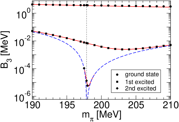
Figure 29: Triton spectrum in the vicinity of a limit cycle as function of the pion mass. The circles, squares, and diamonds give the chiral-potential result of Epelbaum et al. (2006), while the solid lines are N²LO calculations in Pionless EFT Hammer et al. (2007). The vertical dotted line indicates the critical pion mass. The thresholds for stable three-nucleon states are given by the dashed lines. Reprinted by permission from Springer Nature: Hammer et al. (2007), copyright (2007).

V.2 Antinucleon systems

While nucleon-antinucleon pairs can be integrated out at low energies, nuclear EFTs apply as well to systems where antinucleons, a consequence of the Lorentz invariance of QCD, appear in initial states. The simplest such system is antinucleon-nucleon ($\bar{N}\!N$) scattering. While the details of annihilation involve short distances, low-energy antinucleon-nucleus scattering can be described in ways similar to nucleon-nucleus scattering provided that the loss of flux to annihilation is accounted for with complex LECs. Other ingredients are very similar and related by charge conjugation ($C$) to the nuclear potential summarized in Fig. 25.

The use of Chiral EFT for $\bar{p}p$ was pioneered by Chen et al. (2010) and Chen and Ma (2011), along the lines of Kaplan et al. (1996) for the spin-singlet $N\!N$ channel. The $\bar{N}\!N$ potential was derived to $\mathcal{O}(Q^{4}/M_{\text{QCD}}^{4})$ by Kang et al. (2014) and Dai et al. (2017), who also obtained a very successful description of $\bar{p}p$ observables using Weinberg’s prescription together with the promotion of some interactions and the demotion of others. The final-state interactions generated by these potentials Chen et al. (2010); Kang et al. (2015) explain the near-threshold enhancement in the $\bar{p}p$ invariant-mass spectrum seen in charmonium decays and $e^{+}e^{-}$ annihilation. Chiral two-pion exchange had already been incorporated in the partial-wave analysis of elastic and charge-exchange scattering $\bar{p}p$ data by Zhou and Timmermans (2012), following the earlier Nijmegen approach to $N\!N$ Rentmeester et al. (1999, 2003).

V.3 Hypernuclei

Among the “$\cdots$” in Eq. (3) we find the kinetic, mass, and strong and electromagnetic interaction terms of the strange quarks. Chiral EFT can be extended to $SU(3)_{\rm L}\times SU(3)_{\rm R}$ in an attempt to incorporate kaon and eta exchange to describe hypernuclei. The difficulty is the intermediate value of the strange quark mass: it prevents integrating the strange quark out at a perturbative scale, as it is done for heavier quarks, but leads to poor convergence of the ChPT expansion Donoghue et al. (1999) because of the relatively large kaon and eta masses, $m_{K}$ and $m_{\eta}$.

Nevertheless, by counting $m_{K}$ and $m_{\eta}$ as low-energy scales, one can formally apply the power counting of Sec. IV.3.1 to organize the inter-baryon potential along the lines of Sec. IV.3.2. The two-baryon potential was derived up to $\mathcal{O}(Q^{2}/M_{\text{QCD}}^{2})$ by Polinder et al. (2006), Haidenbauer and Meißner (2010), Haidenbauer et al. (2013), and Haidenbauer et al. (2016). With Weinberg’s prescription, a description of hyperon-nucleon data is obtained of quality comparable to the most advanced phenomenological models. The leading three-baryon forces, which appear at $\mathcal{O}(Q^{n+1}/M_{\text{QCD}}^{n+1})$, have also been written down Petschauer et al. (2016). A large-$N_{\rm c}$ analysis of hyperon-nucleon interactions was carried out by Liu et al. (2019), while a covariant formulation presented by Li et al. (2016, 2018). If $m_{K}$ or $m_{\eta}$ are considered large scales, the onset of $\eta$-nuclear binding can be considered in a Pionless EFT approach in order to derive constraints on the $\eta N$ scattering length Barnea et al. (2017a, b).

Certain hypernuclei are also amenable to Pionless and Halo EFT. The process of $\Lambda d$ scattering and the properties of the hypertriton ${}_{\Lambda}^{3}$H in the $SU(3)$ limit were first studied in Pionless EFT by Hammer (2002). Since the hypertriton is extremely shallow, the low-energy observables in this channel are insensitive to the exact values of the $\Lambda N$ low-energy parameters, as any shift can be absorbed by changing the three-body force. By constructing a system of coupled integral equations in the spin-isospin basis, Ando et al. (2015) investigated the viability of the $nn\Lambda$ bound state suggested by the recent experiment of the HypHI collaboration at GSI Rappold et al. (2013). The three-body force present at LO prevented any definitive conclusions about the existence of the $nn\Lambda$ bound state. More recently, Hildenbrand and Hammer (2019) calculated the structure of $nn\Lambda$ and ${}_{\Lambda}^{3}$H, and clarified the value of the corresponding scaling factors. For physical hyperon and nucleon masses, they obtained the $\Lambda d$ scattering length $a_{\Lambda d}=(13.8^{+3.8}_{-2.0})$ fm, where the error is dominated by the uncertainty in the hypertriton binding energy. Implications of three-body universality to systems with two neutrons and a flavored meson (such as $K^{-}$ and $D^{0}$) were considered by Raha et al. (2018).

Pionless EFT for states with strangeness ${-}1$ was extended up to ${}_{\Lambda}^{5}$He by Contessi et al. (2018), presenting a solution to the “overbinding problem” observed with previous approaches based on nucleon-hyperon model interactions. Light nuclear states with strangeness ${-}2$ have also been examined by Contessi et al. (2019). With the $\Lambda\Lambda$ contact interaction estimated from correlations observed in relativistic heavy ion collisions and the $\Lambda\Lambda N$ three-body force constrained by the binding energy of ${}^{\ \ 6}_{\Lambda\Lambda}$He, the conditions for ${}^{3,4}_{\Lambda\Lambda}n$, ${}^{4,5}_{\Lambda\Lambda}$He and ${}^{\ \ 5}_{\Lambda\Lambda}$H binding were discussed.

In paralell, ${}_{\Lambda\Lambda}^{\ \ 4}$H and ${}_{\Lambda\Lambda}^{\ \ 6}$He have been described in Halo EFT as three-body systems where the two hyperons orbit around, respectively, deuteron Ando et al. (2014) and alpha-particle Ando and Oh (2014) cores. In the spin-singlet channel of $S$-wave ${}_{\Lambda}^{\,3}$H-$\Lambda$ scattering, there is no bound state and no three-body force at LO. In this case, the ${}_{\Lambda}^{\,3}$H-$\Lambda$ scattering length was found to be $a_{0}=(16.0\pm 3.0)\leavevmode\nobreak\ \mathrm{fm}$. In the spin-triplet channel, a $\Lambda\Lambda d$ contact interaction is required at LO to obtain a cutoff-independent ${}_{\Lambda\Lambda}^{\ \ 4}$H binding energy. Similarly, a $\Lambda\Lambda\alpha$ three-body force is needed for ${}_{\Lambda\Lambda}^{\ \ 6}$He renormalization already at LO, but the correlation between the double-$\Lambda$ separation energy of ${}_{\Lambda\Lambda}^{\ \ 6}$He and the $S$-wave $\Lambda\Lambda$ scattering length could be investigated.

The paucity of experimental information on hypernuclei represents an important opportunity for Lattice QCD to impact nuclear physics through EFT (see Sec. V.1.1).

V.4 Hadronic molecules

Universality also bridges the gap between the seemingly unrelated domains of atomic and hadronic physics. In recent years, a large number of new “quarkonium” states in the charmonium and bottomonium region have been identified by various experiments Patrignani et al. (2016). Many of these states are close to the thresholds for decays into charm and bottom mesons which strongly influences their properties, see reviews by Swanson (2006) and Brambilla et al. (2011). A new “flavored nuclear physics” has emerged where nucleons are replaced by hadrons containing heavy quarks, which is amenable to EFTs that parallel those deployed in conventional nuclear physics.

A prominent member of this family of so-called $XYZ$ states is the $X(3872)$, where the number in parentheses refers to the center-of-mass energy (in $\mathrm{MeV}$) at which the state was first observed. The closeness of the $X(3872)$ to the $\bar{D}^{0}D^{*0}$ threshold as well as its quantum numbers $J^{PC}=1^{++}$ Aaij et al. (2013) quickly led to the conjecture that it can be interpreted, at least in part, as a shallow bound or virtual state of these two mesons. Braaten and Kusunoki (2004a) first used an EFT assuming a large $\bar{D}^{0}D^{*0}$ scattering length to describe the $X(3872)$, with a number of further papers building upon this, for example Braaten and Kusunoki (2004b); Braaten et al. (2004); Braaten and Kusunoki (2005b, a); Braaten and Lu (2007, 2008). An extension of this EFT to the three-body sector was given by Canham et al. (2009), who studied $D$ and $D^{*}$ scattering off the $X(3872)$. Consequences of this pionless EFT for other states, including the effects of heavy quark symmetry, are discussed by AlFiky et al. (2006); Mehen and Powell (2011); Nieves and Valderrama (2012); Guo et al. (2013a); Wilbring et al. (2013); Guo et al. (2013b); Albaladejo et al. (2015); Valderrama (2018); Liu et al. (2018).

The corrections to universality can be calculated systematically using an EFT for the $X$ with explicit pions, called XEFT, which was developed by Fleming et al. (2007). The analog of the scale (73) is

$$M_{DD^{*}}=\frac{8\pi f_{\pi}^{2}}{g^{2}\mu_{{D^{0}}D^{*0}}}\,,$$ (81)

where $\mu_{{D^{0}}D^{*0}}\simeq 967\leavevmode\nobreak\ \mathrm{MeV}$ is the reduced mass and $g\simeq 0.5-0.7$ is the transition coupling of the pion to $\bar{D}^{0}$-$D^{*0}$. $M_{DD^{*}}$ is larger than $M_{N\!N}$, while the mass associated with OPE is smaller, $[(m_{D^{*0}}-m_{D^{0}})^{2}-m_{\pi}^{2}]^{-1/2}\simeq 45$ MeV instead of $m_{\pi}$. As a consequence, one expects pions to be perturbative Fleming et al. (2007); Baru et al. (2011); Valderrama (2012); Alhakami and Birse (2015); Braaten (2015) in the region of energies where the bound state might lie. XEFT is analogous to the version of Chiral EFT discussed in Sec. IV.4.4.

A number of aspects of exotic mesons were investigated in this approach, such as light-quark-mass Jansen et al. (2014) and finite-volume Jansen et al. (2015) effects on the $X(3872)$ binding energy, various decays of the $X(3872)$ Fleming et al. (2007); Fleming and Mehen (2008); Mehen and Springer (2011); Baru et al. (2011); Fleming and Mehen (2012); Mehen (2015), the decay $\psi(4160)\to X(3872)\gamma$ as a probe the $X(3872)$’s molecular content Margaryan and Springer (2013), the triangle singularity in $e^{+}e^{-}\to X(3872)\gamma$ Braaten et al. (2019b), scattering of low-energy pions on the $X(3872)$ Braaten et al. (2010), the role of exact Galilei invariance for the $X(3872)$ and its line shape Braaten (2015); Schmidt et al. (2018), $X(3872)$ production in colliders Braaten et al. (2018, 2019a), and heavy and light-quark symmetries Hidalgo-Duque et al. (2013).

The role of pion exchange has been further discussed for the $X(3872)$ at physical Nieves and Valderrama (2011); Kalashnikova and Nefediev (2013); Wang and Wang (2013); Baru et al. (2015b) and unphysical Baru et al. (2013, 2015a) quark masses, as well as in the context of other states and the implications of heavy quark symmetry Liu et al. (2014); Cleven et al. (2015); Baru et al. (2016, 2017); Lu et al. (2019); Geng et al. (2018a, b); Xu et al. (2019); Wang et al. (2018, 2019); Baru et al. (2019a).

V.5 Fundamental symmetries

According to QCD, nuclei ultimately emerge from the interaction between quarks and gluons. The quarks and gluons, however, are subject not only to the strong and electromagnetic interactions displayed explicitly in Eq. (3), but also to weak and possibly other interactions found in the “$\cdots$”. Allowing for violation of symmetries such as parity ($P$) and time reversal ($T$) from higher-dimensional interactions in Eq. (3) introduces other components to the nuclear potential and currents. Nuclear EFT enables us to incorporate the effects of weak and beyond-the-Standard-Model interactions in the description of low-energy hadronic and nuclear processes. Input from Lattice QCD is particularly desirable in this context Cirigliano et al. (2019).

V.5.1 Parity violation

Besides being responsible for beta decay, weak interactions also imply that there should be small $P$-violating operators in the nuclear force and currents. Since they stem mostly from four-quark interactions proportional to the Fermi constant $G_{F}\simeq 1.17\cdot 10^{-5}\leavevmode\nobreak\ \mathrm{GeV}^{-2}$, NDA (11) suggests that for $T$-conserving $P$ violation the suppression factor is $G_{F}f_{\pi}^{2}\sim 10^{-7}$. The framework for the incorporation of $P$-violating effects in nuclear EFTs was developed by Zhu et al. (2005). A major motivation for this program is to understand the tension that exists among different experiments Holstein (2010), when analyzed with quark and meson-exchange models Desplanques et al. (1980).

In the pionless theory, $P$ violation in the nuclear force is manifest as $S$-to-$P$-wave contact interactions, five of which are independent at LO Zhu et al. (2005); Girlanda (2008). Phillips et al. (2009) pointed out that Pionless EFT is well suited to describe a number of existing and planned $N\!N$ scattering experiments and calculated the relevant relationships between observables (typically spin-polarization asymmetries) at LO in the $P$-violating sector. Schindler et al. (2016) have argued that large-$N_{\rm c}$ arguments can be used to reduce the number of LO $P$-violating operators from five to two. Grießhammer and Schindler (2010) have shown that no $P$-violating $3N$ force occurs up to and including NLO, enabling predictions for $P$-violating elastic neutron-deuteron scattering Grießhammer et al. (2012b); Vanasse (2012) based on the two-nucleon LECs. However, Vanasse (2019) concludes that a $P$-violating $3N$ force is required at NLO, after all.

First pionless calculations of the deuteron anapole (or toroidal dipole) moment and $P$-violating effects in the $np\to d\gamma$ capture process were presented by Savage (2001), building upon previous work in the theory with explicit, perturbative pions Savage and Springer (1998); Kaplan et al. (1999a); Savage and Springer (2001). Schindler and Springer (2010), Vanasse and Schindler (2014), and Shin et al. (2010) looked at $P$-violating asymmetries in the $np\to d\gamma$ process. Spin polarization in the inverse process was studied by Ando et al. (2011). Moeini Arani and Bayegan (2013) and Arani and Bayegan (2014) studied $P$ violation in the $nd\to{}^{3}\mathrm{H}\,\gamma$ radiative-capture reaction, and Mahboubi et al. (2016) included electromagnetic effects to calculate polarized $pd$ scattering.

Some of these processes have also been considered in Chiral EFT. As far as strong interactions are concerned, the power $\mu$ of a contribution to the potential (see Eq. (IV.3.1)) can now be negative, but of course the corresponding terms are suppressed by small factors. The lowest orders of the $T$-conserving, $P$-violating potential and electromagnetic currents were obtained by Zhu et al. (2005), Kaiser (2007), Liu and Zhu (2008), Girlanda (2008), Viviani et al. (2014), and de Vries et al. (2014). They display new elements, such as TPE, compared to the one-meson-exchange potentials usually employed to study $P$ violation Desplanques et al. (1980). Calculations of $P$ violation in few-nucleon systems have so far been based on Weinberg’s prescription, as reviewed by de Vries and Meißner (2016).

V.5.2 Time-reversal violation

In the case of $T$, there is potential violation from the QCD vacuum angle $\bar{\theta}$ and from higher-dimensional operators, all contained in the “$\cdots$” in Eq. (3). While the former is anomalously small ($\bar{\theta}\stackrel{{\scriptstyle<}}{{{}_{\sim}}}10^{-10}$ Tanabashi et al. (2018)), the latter are suppressed by at least two powers of a large scale. All violation from operators of dimension up to six is accompanied by $P$ violation. These interactions induce $T$-violating nuclear form factors, such as electric dipole and magnetic quadrupole, which could be probed in proposed storage-ring experiments Pretz (2013). In nuclear EFT they are calculated within the same framework used for nucleon electric dipole moments.

The lowest-order $P,T$-violating potential calculated in Chiral EFT by Maekawa et al. (2011) and de Vries et al. (2013) shows, as its $P$-conserving counterpart, new ingredients compared to one-meson-exchange potentials Liu and Timmermans (2004). The implications of an additional large-$N_{\rm c}$ expansion are discussed by Samart et al. (2016). Together with $P,T$-violating currents, form factors were calculated for the deuteron in Chiral EFT with perturbative pions by de Vries et al. (2011b) and with Weinberg’s prescription by de Vries et al. (2011a), Bsaisou et al. (2013), Liu et al. (2012), and Bsaisou et al. (2015); good accord was found between these calculations. de Vries et al. (2011a) and Bsaisou et al. (2015) have also calculated the electric dipole moments of triton and helion with Weinberg’s prescription. The deuteron also possesses a $P$-conserving, $T$-violating form factor, the toroidal quadrupole. The contribution to this moment from the same $P,T$-violating operators in conjunction with weak interactions was obtained with perturbative pions by Mereghetti et al. (2013). $T$ violation in few-nucleon systems is reviewed by Mereghetti and van Kolck (2015), where it is shown how measurements of the electric dipole moments of nuclei, together with further theoretical advances, could at least partially disentangle the various possible sources of $T$ violation.

V.5.3 Other symmetries

Higher-dimensional operators in the Standard Model break also other symmetries like lepton ($L$) and baryon ($B$) number, but less work exists in the context of nuclear EFTs. Of particular contemporary interest is $L$ violation, especially through the only dimension-five operator, which leads to Majorana neutrino masses. The most sensitive laboratory probe of $L$ violation (by two units) is neutrinoless double-beta decay ($0\nu\beta\beta$), which is however afflicted by severe nuclear-physics uncertainties. Traditionally $0\nu\beta\beta$ has been calculated from the exchange of an explicit Majorana neutrino together with phenomenological nuclear models, but more recently nuclear EFTs have been deployed Cirigliano et al. (2018c). It has been uncovered that a short-range LEC must enter at LO for proper renormalization in both Pionless Cirigliano et al. (2018b) and Chiral Cirigliano et al. (2018a) EFTs. First ab initio calculations of these contributions in light nuclei are becoming available Pastore et al. (2018); Cirigliano et al. (2018a). Operators of higher dimensions have been considered as well Prezeau et al. (2003); Cirigliano et al. (2017). Implementation of these operators in the shell model are starting to appear Horoi and Neacsu (2017, 2018).

Analogous to $L$ violation is $B$ violation by two units. The process of neutron-antineutron oscillation in a nucleus leads to decay after the antineutron annihilates with a nucleon. An NLO calculation of this process in the deuteron Oosterhof et al. (2019) gives a lifetime in Pionless EFT that is comparable to earlier zero-range models, while in Chiral EFT (with perturbative pions) it is a factor of $\simeq 2.5$ smaller than existing potential-model calculations.

Extensions of the Standard Model can be constructed which account for possible violation of Lorentz and (then unprotected) $CPT$ symmetries at high energies, allowing for operators with low dimensions. Most tests of these symmetries take place at low energies where QCD is nonperturbative, impeding direct bounds on operators involving strongly-interacting particles. Among the lowest-dimensional operators of this type is a Lorentz-violating (but $CPT$-conserving) purely gluonic operator. The nuclear potential induced by this operator and its possible effects on atomic-clock comparisons and on the spin precession of the deuteron and other light nuclei in storage-ring experiments are discussed by Noordmans (2017). Dimension-five operators are similarly discussed by Noordmans et al. (2016). A more detailed analysis of the nuclear implications of these interactions is needed.

V.6 Dark-matter detection

Nuclear EFTs have also been used to describe dark-matter scattering off heavy nuclei in direct-detection experiments. The dark-matter particles must be nonrelativistic in order to be bound in the dark-matter halo by gravitation, with typical velocities of order $0.001$ times the speed of light. Since the recoil momentum is comparable to the typical momentum of a nucleon in the nucleus, it is crucial for the interpretation of current experimental limits (cf. Liu et al. (2017)) that nuclear-structure factors be properly addressed.

The calculation of nuclear-structure factors in nuclear EFT has been organized in two different ways. First, a Pionless EFT for nucleon and dark-matter fields Fan et al. (2010); Fitzpatrick et al. (2013, 2012); Anand et al. (2014) allows a study of nuclear response functions in terms of effective couplings, and the extraction of limits on the coefficients of the operators. This approach reaches its limit at the largest momentum transfers for scattering off heavy nuclei where the details of pion exchange are resolved. Second, Chiral EFT has been used to predict the nuclear-structure factors for spin-independent and spin-dependent scattering. The analysis within Chiral EFT establishes relations between different operators in the pionless framework, and provides a counting scheme that indicates at which order two-nucleon operators contribute. Recent work in this direction includes Chiral EFT-based structure factors for the spin-dependent response Menendez et al. (2012); Klos et al. (2013), aspects of spin-independent scattering Cirigliano et al. (2012, 2014); Vietze et al. (2015), scattering off light nuclei Körber et al. (2017), inelastic scattering Baudis et al. (2013), as well as a general Chiral EFT analysis of one- and two-body currents Hoferichter et al. (2015b, 2016, 2019) and improved limits for dark-matter models from experimental searches Hoferichter et al. (2017); Aprile et al. (2019).

V.7 Bosons with large scattering length

Up to technical details that arise from spin and isospin degrees of freedom, Pionless EFT is virtually identical to a theory that describes a system of bosons with a large two-body scattering length. Throughout the history of Pionless EFT this fact has been used repeatedly, the few-boson system serving to guide analogous analyses in the few-nucleon sector.

But such bosonic systems are relevant far beyond serving as a toy problem. Experimentally, they are realized in cold atomic gases, where the two-body interaction can in fact be tuned arbitrarily by varying an external magnetic field—the Feshbach-resonance mechanism. In particular, the Efimov effect has been established experimentally by exploiting the fact that the occurrence of three-body states close to points where the two-body scattering length is tuned to infinity Kraemer et al. (2006), with many more experiments since the first observation. A comprehensive discussion of the theoretical treatment of universal few-body systems has been given by Braaten and Hammer (2006). The current status of the field was recently reviewed by Naidon and Endo (2017).

VI Conclusion

As shown in Fig. 1, a significant portion of low-energy nuclear physics is amenable to an EFT description, with different theories tailored specifically for different regions. With increasing energy, a tower of EFTs starts from the simple pionless case, an expansion around the unitary limit of large $N\!N$ scattering lengths. Its range of applicability can be extended by the inclusion of pions—first perturbatively then nonperturbatively—in Chiral EFT, constructed as an expansion around the eponymous chiral limit of vanishing quark masses. Although there is a fundamental difference regarding how pions are treated—a heavy degree of freedom in Pionless EFT, but a light one in Chiral EFT—these theories are low-energy limits of QCD. They are both formulated as theories of pointlike nucleons with interactions that give rise to low-energy poles of the $S$ matrix.

The fact that nucleons, being composite hadrons, in reality have substructure is encoded in the EFT expansion, namely in local operators with an increasing number of derivatives. Establishing the ordering of such interactions is the crucial element that enables a systematic description of observables.

The usefulness of EFT does not stop at this point because new scale separations arise in nuclei. A particular case, Halo/Cluster EFT, has been discussed in this review as a promising way to describe cluster-like nuclei. On yet another level, efforts are underway to construct EFTs for rotational and vibrational modes in heavy nuclei Papenbrock (2011). Moreover, applications to other composite systems—from dark matter to cold atoms—show how nonperturbative EFTs are a driving force behind many important developments in modern theoretical physics.

EFTs are ideally suited to root nuclear physics in the Standard Model EFT, elegantly exploiting its emergence from QCD as the underlying theory of the strong interaction—particularly through lattice simulations. EFTs have become the initio of ab initio methods for the solution of few- and many-nucleon dynamics and engendered such an explosion of activity that it is difficult to draw a line to conclude this article. We have already reached the point where calculated nuclear properties are being used to identify deficiencies in the nuclear interactions used as input.

Ab initio calculations now almost unanimously follow—mostly in Chiral EFT, but increasingly in Pionless EFT—Weinberg’s original prescription, i.e., they do not expand on the subleading components of the potential. Our emphasis in this review were approaches that pursue the longstanding goal of RG invariance through the perturbative expansion of the $S$ matrix on the subleading interactions. This approach has led to a new and unified description of few-body “Efimov physics” under the umbrella of Pionless EFT. It remains to establish, however, to which extent this framework can share the efficiency of Weinberg’s approach without dependence on the form of the regulator, or perhaps explain its phenomenological success for larger nuclei within narrow cutoff windows.

It is thus our hope that this review does not only provide a unified overview of what has been done, but will also inspire future research towards a comprehensive and solid understanding of nuclear structure and reactions from an EFT, and ultimately QCD, perspective.