Kinetics of coarsening have dramatic effects on the microstructure: self-similarity breakdown induced by viscosity contrast.

Abstract

The viscous coarsening of a phase separated mixture is studied and the effects of the viscosity contrast between the phases are investigated. From an analysis of the microstructure, it appears that for moderate departure from the perfectly symmetric regime the self-similar bicontinuous regime is robust. However, the connectivity of one phase decreases when its volume fraction decreases or when it is becoming less viscous than the complementary phase. Eventually self-similarity breakdown is observed and characterized.

I Introduction

The phase separation and the subsequent coarsening of the microstructure under the effects of the surface tension is an ubiquitous mechanism in industrial processesLevitz et al. (1991); Craievich et al. (1986); Kumar and Weinhold (1996). In this context understanding how patterns are formed and how they can be controlled is highly desirable. However this process is complex and involves different mechanisms. Indeed, after a quench an initially thermodynamically stable mixture will lose stabilityCahn and Hilliard (1958), it will then phase separate spontaneously through spinodal decompositionCahn (1965). In both cases, after the initial phase separation process, a complex microstructure has spontaneously formed. It is constituted of the two phases that are separated by an interface with a huge surface area. The evolution of the system will then be driven by the surface tension and will lead to an increase of the characteristic lengthscale of the pattern $l$. If both phases are liquid, the coarsening process involves two successive regimes. First, when $l$ is small the coarsening is mostly due to diffusion and $l$ grows as $t^{1/3}$Cahn (1966); Lifshitz and Slyozokov (1961); Kwon et al. (2007, 2010); Puri et al. (1997); Sun et al. (2018), thereafter, when $l$ is large the effects of fluid flow become dominantWong and Knobler (1981); Siggia (1979); Appert et al. (1995); Bastea and Lebowitz (1997); Kendon et al. (2001); Tanaka and Araki (1998) and $l$ grows as $t$. Hence the time evolution of the characteristic lengthscale of the microstructure is well understood. However, the understanding of the microstructure itself and of how it can be controlled is limited. Indeed, the volume fraction of the phases can be used to control the microstructure and for instance by properly choosing volume fractions of the phases, one can tune a transition from a bicontinuous microstructures where both phases are percolating clusters to an inclusions in a matrix pattern.

This approach is mainly focused on the initial phase separation process and overlooks the importance of the kinetics of the coarsening process, which is well exemplified by recent experiments on the viscous coarsening of glassesBouttes et al. (2014, 2016). Indeed it has been shown that the microstructure is affected by both the volume fraction of the phases and their relative viscosities. Hence, while the driving force for coarsening is always the reduction of the surface energy, the kinetic of the coarsening, that is the path taken by the system to dissipate energy, has a dramatic effect on the microstructure. For instance if the volume fraction of the minority phase is close to $0.3$, when it is much more viscous than the majority phase, a bicontinuous microstructure remains during coarsening while if it is much less viscous a transition toward a discontinuous microstructure is observed. This is in line with previous theoretical work where the interplay between diffusion and flow during the initial stage of spinodal composition was studiedTanaka and Araki (1998) or where visco-elastic effects were taken into accountTanaka (2000); Araki and Tanaka (2000); Kumar and Weinhold (1996)

Here, we focus on the late stage of coarsening in liquids where the pattern evolution is due to viscous flow (diffusion can be neglected) and where the inertial effects are also negligible. Using numerical simulations we show that tuning the kinetic of the coarsening process through the viscosity ratio between the phases dramatically changes the microstructure. The paper is organised as follows. First we present the model equation, the numerical methods and the choice of the initial conditions and of parameters in the light of the physics of the coarsening process. We also describe briefly the tools that have been used to describe the microstructure. Thereafter we present the numerical results in the case where the self-similar coarsening is robust and we discuss its loss of stability. Finally we conclude.

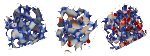
Figure 1: Typical images of the interface between the phases for different values of the parameters. The color of the surface indicates the gaussian curvature (blue: negative, red: positive). One can see that the regions with positive gaussian curvature are more present in the later case.

II Method

The thermodynamics of a binary fluid is well described by the diffuse interface theory of Cahn and HilliardCahn and Hilliard (1958). The simplest symmetric form of the Cahn-Hilliard free-energy reads as:

$$\mathcal{F}=\int\epsilon^{2}(\nabla c)^{2}+A(c^{2}(c-1)^{2})$$ (1)

With such a choice, when $A>0$, an homogeneous mixture with a composition close to 0.5 will spontaneously phase separate into two phases with concentration 0 and 1. The surface tension associated to the interface between the phases and its thickness can be chosen by adjusting $A$ and $\epsilon$. Here $\epsilon^{2}=2.56$ and $A=4.$ were chosen so that $\gamma\approx 0.75$Kendon et al. (2001) and so that the interface thickness is of the order of $w_{int}=1.6$Cahn and Hilliard (1958). The coarsening dynamics via convection and diffusion is governed by the coupled Navier-Stokes (eq.II) and the convective Cahn-Hilliard (CH) (eq.2) equations (NSCH), also known as model H Hohenberg and Halperin (1977). The Navier-Stokes/Cahn-HilliardAnderson et al. (1998) model was used along with the incompressibility constraint (eq.4):

$$\partial_{t}c+\mathbf{v}\cdot\nabla c = -M\triangle\mu$$ (2)

$$\partial_{t}\mathbf{v}+\nabla\cdot(\mathbf{v}\otimes\mathbf{v}) = {\frac{-1}{\rho}(\nabla p+c\nabla\mu)}$$

$$+ \nabla\cdot\left(\frac{\nu{(c)}}{2}(\nabla\mathbf{v}+\nabla\mathbf{v}^{T})\right)$$

$$\nabla\cdot\mathbf{v} = 0$$ (4)

In the Cahn-Hilliard equation (Eq. 2), $M$ is the mobility, $\mu=\delta\mathcal{F}/\delta c$ is the chemical potential that derives from the CH free energy.

In the Navier-Stokes equation (Eq. II) the $-\nabla p$ term on the RHS includes a Lagrangian multiplier that forces incompressibility. The second term is the thermodynamic stress, and accounts for capillary forces. The last term accounts for the viscous dissipation with a composition dependent kinematic viscosity:

$$\nu{(c)}=(1-c)\nu_{1}+c\ \nu_{2},$$ (5)

where $\nu_{1}$ and $\nu_{2}$ are the viscosities of the two phases corresponding to $c=0$ and $c=1$. The viscosity contrast is then defined as $VC=\nu_{1}/\nu_{2}$ The mass density is $\rho$. The model equations were simulated numerically using standard approachesOrszag (1969); Orszag and Patterson (1972); Liu and Shen (2003); Zhu et al. (1999) that are described in the supplementary material ofHenry and Tegze (2018) together with a more detailed description of the model equations that is inspired by Shang et al. (2011); Tóth et al. (2016).

The NSCH model reproduces well the initial phase separation followed by the coarsening of the microstructure that is due to diffusion at small length-scales with a characteristic length-scale growing as $l\propto t^{1/3}$Lifshitz and Slyozokov (1961); Cahn (1966). At larger length scales the coarsening is driven by convection that is governed by surface tension and viscous dissipation. As a result $l$ grows linearly: $l=v_{0}t\propto\gamma/\nu t$ Siggia (1979) where $\gamma$ is the surface tension and $\nu$ is the viscosity of the fluid when $VC=1$. The transition from the diffusive growth to a viscous growth occurs when $v_{0}$ is much larger than the growth velocity associated with diffusion (which itself is a function of the mobility of chemical species and of the chemical potential difference induced by the Gibbs effect). This translates into the fact that the Péclet number ($Pe=lv_{0}/M/\gamma$) is large. Finally the viscous growth law looses its validity when inertial effects cannot be neglected (the Reynolds number $Re$, defined as $l/l_{0}$ where $l_{0}=\nu^{2}/(\gamma\rho)$ becomes large). Since, we are considering fluids with different viscosities, two Reynolds number can be computed: one for each phase. Since the fluid flow in both phases share the same velocity and since there is a clear relation between the fluid flow velocity and the effective viscosity $\nu_{eff}=\sqrt{\nu_{0}\nu_{1}}$Henry and Tegze (2018), the Reynolds number in each phases writes $Re_{1,2}=l/(\nu_{eff}^{2}\gamma\rho VC^{\pm 1/2})$.

Here we have limited ourselves to the viscous coarsening of an already phase separated mixture, assuming that the viscosity is sufficiently high to avoid the effects of fluid flow during the initial phase separation and before well defined phases are present and coarsening takes placeTanaka and Araki (1998). It is important to note that during the course of the coarsening, since $l$ is growing, these two numbers grow (proportionally to $l$). As a result, during the coarsening of a bicontinuous structure, both $Pe$ and $Re$ will increase and there is a transition from a diffusive coarsening regime where ($Pe<<1$, $Re<<1$) to a viscous dominated regime ($Pe>>1$ and $Re<<1$) followed by an inertia dominated regime ($Pe<<1$, $Re>>1$)Kendon et al. (1999). Here we have focused on the well defined Siggia regime for which $Pe>>1$ and $Re<<1$. These constraints apply on the macroscopic lengthscale. In contrast with this requirement, at the scale of the interface, the flow deforms the concentration profile through the interface and therefore changes the surface tension. This effect is unwanted and needs to be counterbalanced by an appropriate restoring mechanism. In actual systems this mechanism is diffusion which is effective on the scale of the actual interface thickness. Here, in order to allow computations, the interface thickness is increased, and some care must be taken to ensure that the diffusion is still efficient enough to restore the equilibrium profile. This translates into the fact that the interface Péclet number must be small enough. According to these constraints and using the results of Henry and Tegze (2018) we have chosen $\rho=1$, $\nu_{eff}=\sqrt{\nu_{0}\nu_{1}}=8$ and a mobility of $M=0.0625$. With this choice of parameters and viscosity contrasts ranging from 1 to 128 both the inertial and diffusive effects can be neglected during coarsening for system characteristic length ranging from $\approx 20$ to $200$. However, when considering viscosity contrast significantly higher than 128, the decrease of the viscosity of the fluid phase is likely to lead to significant a departure from the ideal low Re regime with parameters used here. In the case of experimental systems presented in Bouttes et al. (2014), the viscosities of both phases are such that they are both in the low $Re$ regime.

In our simulations the grid spacing is set to 1 and time step $\Delta t$ is also set to 1. Typical domain size is $1024^{3}$ which ensures that finite size effects are negligible.

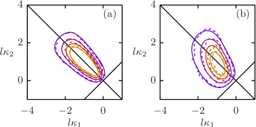
Figure 2: . Contour plot of the PDFs of the principal curvature for a volume fraction of $\varphi=0.5$ for two value of the viscosity contrast $VC=1$ (a) and $VC=128$ (b). The contour lines are equally spaced.Taken fromHenry and Tegze (2018).Contours have been taken at two distinct times corresponding to (solid) $l\approx 23$ in (a) ( resp. 30 in (b)) and to (dashed) $l\approx 88$ in (a) (resp.84 in (b) ) (dashed).

The constraints on the macroscopic Péclet number and on the interface Péclet number imply that the initial phase separation is always affected by the flow and by the viscosity contrast between the two phases. Therefore, we have chosen to use initial conditions that were computed through a well defined procedure (described in appendix). This approach allows us to focus on the effects of the coarsening process itself and had the advantage to allow to build different microstructures with different statistical properties in order to test the robustness of the self similar regime by showing whether the same self similar regime is reached from two different initial conditions that are not simply two realizations of the same stochastic process. During the build up of the initial condition the volume fraction of the phase 1, $\varphi$ is set.

Finally we present briefly the tools of analysis that were used here. As in our previous workHenry and Tegze (2018), the microstructure is first characterized by a characteristic lengthscale $l$ that is computed as the ratio between the total volume and the total interface between the phases. More precisely, it is defined using an energetic approach:

$$l=\frac{V\gamma}{\int\epsilon^{2}(\nabla c)^{2}}$$ (6)

which gives actually $l=V/S$ when the interface between the phases corresponds to an equilibrium profile. In order to characterize more finely the microstructure other quantities are studied. The geometry of the pattern is described using the statistical properties of the curvature of the interface between the phases. From the field of the implicitly defined interface, the curvature are computed using implicit formulasGoldman (2005). The Probability Distribution functions of the principal curvatures are then determined as inHenry and Tegze (2018); Kwon et al. (2007, 2010). A typical example of the PDFs contour that will be used as a reference in the following is shown in fig. 2. In addition integral quantities are considered: the averaged mean curvature rescaled by $l$ and the rescaled genius number: $g=l^{2}(1-\int_{V}\kappa_{g}/(4\pi))/S$ where $\kappa_{g}=\kappa_{1}\kappa_{2}$ is the Gaussian curvature of the interface. The Gaussian curvature is independent of the orientation of the interface and the genius number $g_{l}=(1-\int_{V}\kappa_{g}/(4\pi))$ is a topological invariant of the pattern which is directly related to its Euler’s characteristic. The orientation of the surface is chosen so that the normal points toward the inside of the phase for which the volume fraction is given.

In addition, the conductance $\mathcal{G}$ of the microstructure under the assumption that one phase is conducting and the other is isolating (details of the computation and of the numerical method are given in appendix) is also computed. This quantity gives an estimate of the connectivity of the phase. Indeed, when the phase is non percolating it goes to zero while when it is percolating it can be viewed as the averaged total surface area of the channels that go from one side of the system to the other.

III Results

During the course of our simulations two distinct regimes have been observed. The first one is a continuation of the regime previously described Henry and Tegze (2018) for the case where the volume fraction is 0.5. However, considering volume fractions that differ from $0.5$ leads to more dramatic effects of the changes in flow parameters. Indeed, the system properties are invariant by the transformation :

$$\begin{array}[]{rcl}c&\to&1-c\\ \nu_{1}&\to&\nu_{2}\\ \nu_{2}&\to&\nu_{1}\end{array}$$ (7)

This implies that when changing $\varphi$ to $0.5+(0.5-\varphi)$ and $VC$ ($\log VC$) to $1/VC$ ($-\log VC$), the quantities that depend on the orientation of the interface such as the mean average curvature $<\kappa_{m}>$ are transformed into $-<\kappa_{m}>$ while quantities such as the average Gaussian curvature $<\kappa_{g}>$ that are independent of the interface orientation are transformed into $<\kappa_{g}>$. As a result in the parameter space ($\varphi,\ \log VC$), ($\varphi=0.5$, $VC=1$) is a center of symmetry that corresponds to a point where the interface has zero averrage mean curvature and to an extremum of the averrage gaussian curvature As a result the vicinity of ($\varphi=0.5$, $VC=1$) reflects the symmetries of the problem: more specifically, the average Gaussian curvature when changing parameters is marginally affected which implies that the connectivity of the bicontinuous structure is mostly unchanged. In the following we will show that in the more general case where $\varphi\neq 0.5$ this is no longer the case in the self similar regime. In addition we will present a description of the loss of stability of the self similar-regime and give a rationale for the transition inspired by Bouttes et al. (2016).

III.1 The self similar regime

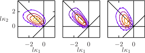
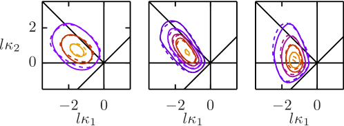
Figure 3: contour plot of the PDFs of the principal curvatures for $\varphi=0.45$ (top) and $\varphi=0.35$ (bottom) and $VC$ equal to 1/128 , 1 , and 128 from left to right. The sign convention is chosen so that the negative curvatures correspond to center of curvature in the minority phase (normal vector pointing toward the minority phase). One can see that there is a clear change in the shape of the distribution. Nevertheless, the self-similar nature of the coarsening regime is illustrated by the fact that the rescaled PDFs are independent of the characteristic size of the microstructure for two different values of the characteristic length.

For a wide parameter range around the perfectly symmetric case, an initially bicontinuous structure evolves after a transient regime in a self-similar manner as it has been described previously. The morphology of the self-similar structure is affected by the control parameters (the volume fraction of the phase ’1 and the ratio of the viscosities of the phase 1 and of the phase 2). In order to give a clear picture of the effects of varying both parameters, we will describe the effects of changing the relative viscosity of the majority phase with respect to the minority phase for a given value of its volume fraction. We will also describe the effects of changing the volume fraction for a given relative viscosity of the less viscous phase with respect to the more viscous one. One should note that while the former approach had already been presented in a previous work it was restricted to variations around the symmetric point and it was limited to a volume fraction of 0.5. This, because of symmetries, implied that the range over which the ratio of viscosities could be varied was limited to two order of magnitudes (between 1 and 128 ). Here since we no longer consider the perfectly symmetric case, the range over which the ratio can be varied is 4 orders of magnitude (between 1/128 and 128). In addition, the parameter value $VC=1$ is no longer a center of symmetry. Hence, thanks to the departure from the vicinity of the center of symmetry and to the wider range of viscosity contrast that can be explored, more visible changes of the microstructure induced by tuning the flow parameters are expected.

This is well illustrated in figure 1 where, for three different values of the viscosity contrast between the phases, the interface between the two phases is plotted at a time of a simulation where the self-similar regime is established and for approximately the same characteristic lengthscales $l$. The volume fraction of the minority phase is $\varphi=0.3$ and the interface is plotted (and coloured proportionally to its Gaussian curvature) when it is 4 times more viscous, 4 times less and 16 times less viscous than the majority phase. From these picture, it is clear that the microstructure are different. When the minority phase is more viscous, regions of positive Gaussian curvature can hardly be seen on the interface. On the contrary, when the minority phase is made less viscous the surface area of regions with positive Gaussian curvature on the interface is increasing. It should also be noted that these regions correspond to spherical caps of the minority phase protruding in the majority phase(both $\kappa_{1,2}<0$). Hence when decreasing the relative viscosity of the minority phase, the microstructure is evolving from a structure that is a network of capillary bridges that are close to minimal surfaces with zero mean curvature and negative Gaussian curvature to a similar structure with the addition of multiple buds of the minority phase protruding in the majority phase.

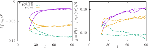
Figure 4: Evolution as a function of the characteristic length of the rescaled mean curvature (left) and genius (right) for the same volume fraction $\varphi=0.40$ and different values of the viscosity ratios. For each value of the viscosity ratio two simulations are represented with different initial conditions and different initial values of the genius and average mean curvature.

In the following parts of this section we will present evidences of the self-similar nature of the coarsening regime and quantitative measures of the effects of changing the viscosity contrast and the volume fraction on the microstructure. The self similar nature of the coarsening regime is well illustrated in figure 3 where the contour of the PDFs of the rescaled principal curvatures are plotted for different values of the viscosity contrast and volume fraction ($\varphi=0.45$ and $\varphi=0.35$). On each plot contours have been plotted at different times corresponding to $l\approx 40$ and $l\approx 80$ and they superimpose well, which indicates that the coarsening process is self-similar as it was for $\varphi=0.5$. The effects on the patterns of changing both the volume fraction and the viscosity contrast are detailed in the following.

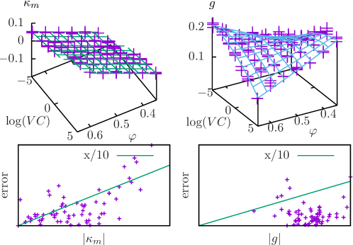
Figure 5: Plot of the rescaled genius and mean curvature as a function of the volume fraction of the phase 1 and the log of the viscosity contrast. The surfaces correspond polynomial fit of the computed values. The bottom plot correspond to the absolute difference between the computed values and the interpolating surface that is represented. One can see that the relative error is of the order of 1/10 in both cases.

When the volume fraction is $\varphi=0.45$, close to $\varphi=0.5$, the PDFs are very similar to the one presented inHenry and Tegze (2018) and recalled in fig.2. On each plot two rescaled PDFs taken for $l\approx 40$ and $l\approx 80$ are represented and superimpose well. For $VC=1$, the PDF is simply slightly shifted away from the zero mean curvature axis $y=-x$ that is a symmetry axis of the PDF for $\varphi=0.5,\ VC=1$ and for $VC=128,\ 1/128$, they are also not very different. One should however, note that in the case $VC=128$, the part of the PDF that corresponds to a positive Gaussian curvature corresponds to caps of the minority phase (the least viscous) protruding in the majority phase while for $VC=1/128$, it corresponds to caps of the majority phase (the least viscous) protruding in the minority phase.

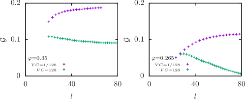
Figure 6: Conductance of the minority phase during the coarsening for two values of the viscosity contrast and two values of the volume fraction.

For a smaller volume fraction $\varphi=0.35$, if both phases share the same viscosity there is no significant departure from the shape presented for $\varphi=0.45$. The shift from the symmetry axis is simply more pronounced. When the minority phase is significantly less viscous ($VC=128$), a significant part of the interface corresponds to region of positive Gaussian curvature. Hence, as can be seen in fig.1, an important part of the minority phase consists of protrusions in the majority phase that do not participate to the connectivity of the minority phase cluster. In the case where $VC=1/128$, the PDF maximum is close to the $\kappa_{2}=0$ axis that corresponds to cylindrical part of the interface (and zero Gaussian curvature). This corresponds to the very thin filament that can be seen for instance in in figure8(d).

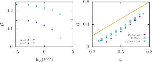
Figure 7: Left Conductance of the sample as a function of the logarithm of the viscosity contrast for two values of the volume fraction $\varphi$. Right: conductance as a function of the volume fraction when the viscosity of the conducting phase is 128, 1 and 1/128 times the viscosity of the isolating phase. The straight line corresponds to $\mathcal{G}=\varphi$

In figure 4 the evolution of the average rescaled mean and Gaussian curvatures are plotted as a function of the characteristic length during coarsening for $\varphi=0.40$, different flow conditions (each line type corresponds to a given flow condition) and different initial conditions (this is made clear by the fact that the lines start at different values of $l\kappa_{m}$ and $g$). In both cases, after a transient that corresponds roughly to doubling $l$ a stationary regime is reached and the limit values of the average Gaussian and mean curvatures are functions of the flow parameters and volume fraction and are independent of the initial condition. This convergence allows to compute the rescaled mean curvature and genius as functions of the viscosity contrast and the volume fraction. The results are summarized in fig. 5, for the range of parameters considered here. The mean curvature is very well approximated by a plane. The rescaled genius plot shows that the center of symmetry $\varphi=0.5,\ VC=1$ is not an extremum but a saddle point. However, despite the fact that the genius is a topological invariant, interpreting this plot in terms of connectivity of the microstructure is difficult.

In order to actually quantify the effects of the control parameters on the connectivity, we have computed the electrical conductance of the microstructure assuming that one phase is conducting (with conductivity 1) while the other is isolating (with conductivity $\approx 0$), the values of the domain size are chosen so that the conductance of a sample filled with the conducting phase is 1 (details are given in the appendix). In fig. 6 (a) the evolution of the conductance of the microstructure as a function of $l$ is plotted for two values of the viscosity contrast and a value of the volume fraction of the conducting phase $\varphi=0.35$. The plot indicates that the conductance is converging toward a limiting value during the coarsening and that the higher conductance is reached by the more viscous phase.

This is confirmed by the plot of the conductance as a function of the viscosity contrast $VC=\nu_{/}1/\nu_{2}$ where the phase 1 is conducting while the phase 2 is isolating for $\varphi=0.3$ and $\varphi=0.4$ in fig. 7. One can see that when decreasing the contrast of the minority phase (which is conducting), there is first a region for which the conductance is not changing a lot while the morphology is changing as is seen on the PDFs of the curvatures or on the evolution of the average mean curvature. Then when the viscosity is decreased further, the conductance decreases significantly. Since the conductance of the phase 1 cannot be larger than its volume fraction (with the conventions used here), the existence of the aforementioned plateau is obvious. Our simulations did not allow to explore systematically the effects of varying the volume fraction on the position of the threshold.

Finally in fig. 7 we have plotted the conductance $\mathcal{G}$ as a function of $\varphi$ for different values of the viscosity contrast. It is clear that, for a given value of $VC$, there is a threshold of the volume fraction below which the conductance of the minority phase goes to zero. This implies that the microstructure is no longer bicontinuous and that the coarsening regime is no longer a self similar viscous regime. The computed conductances when approaching this transition point are decreasing linearly a function of the control parameter (either $\varphi$ or $\log(VC)$ ) down to very small values of the conductance. This indicate that it is likely that the transition from the bicontinuous phase to the inclusion in a matrix phase is continuous: there is no threshold parameter (e.g. $\varphi$ for a given $VC$) above which there exist a bicontinuous phase with a finite conductance and below which the conductance goes to zero. As a result the limits of the self-similar regime should correspond to the domain where $\mathcal{G}(\Phi,VC)=0$ which can be extrapolated using the curves in fig. 7. However, such an extrapolation is likely to give unphysical results when $\varphi$ is close to 1 or to 0 and must be taken with care.

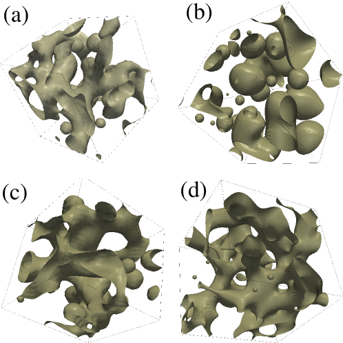
Figure 8: (a),(b) snapshot of the microstructure corresponding to (a) and (d) in fig. 9. (c) and (d) correspond to (e) and (h) in fig. 9. In all snapshots a portion of the domain of size proportional to the characteristic lengthscale $l$ is shown.

Now we give a short description of the transition from a bicontinuous microstructure toward an inclusions in matrix pattern. To this purpose we consider the evolution of an initially bicontinuous pattern when the volume fraction of the minority phase is 0.265. For this value of the volume fraction, there is a self-similar coarsening regime when the minority phase is 128 times more viscous than the majority phase as can be seen in fig 9 and 8. Starting from a microstructure obtained in this regime we let the system evolve with a minority phase that is 128 times less viscous than the majority phase. Snapshots of the microstructure and of the PDFs of the principal curvatures during its evolution are represented in in fig 9 and 8 . For the sake of readability, the snapshots of the microstructure have been taken using portions of the simulation domain of varying size proportionally to the characteristic length $l$. Both the snapshots and the PDFs show that starting from a bicontinuous pattern that consists of capillary bridges linked in a network, the microstructure evolves toward a pattern where there are less capillary bridges and more spherical caps on the microstructure. This evolution eventually leads to the formation of multiple inclusions of the minority phase isolated in the majority phase. In fig. 6 the changes in the conductance of the microstructure during this evolution are plotted and there is a linear decrease of $G$ with $L$ until $G$ reaches zero, which indicates that the minority phase is no longer percolating. It should also be noted that during the time evolution from a bicontinous structure to an incluions in a mattrix pattern, neither the averrage mean curvature nor the the averrage gaussian curvature (see fig. 10) present a discontinuity. They vary smoothly: when the self similar regime is unstable, the mean curvature and the gaussian curvature decrease linearly with time. When considering the two curves it is impossible to detect the loss of continuity of the microstructure. Hence, since the genius is a topological invariant, this confirms that the evolution of the network is continuous in time in the large system size limit.

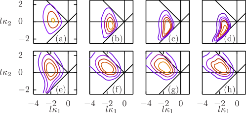
Figure 9: a, b, c and d: Evolution of the PDFs of curvatures for $\varphi=0.735$ when the minority phase is 128 times less viscous than the majority phase. The PDFs is initially centered relatively close to the $\kappa_{1}=-\kappa_{2}$ line. The evolution is such that it is moving toward the line $\kappa_{1}=\kappa_{2}<0$ that corresponds to inclusions of the minority phase in the majority phase. e, f, g and h: the same evolution when the minority phase is the more viscous one. There is a clear evolution toward a distribution centered close to the $\kappa_{1}=-\kappa_{2}$ line (that corresponds to $\kappa_{m}=0$ that appears to be almost unaffected by the changes in $l$.

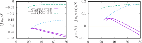
Figure 10: Evolution with characteristic length of the mean curvature (left) and rescaled genius (right)for the same volume fraction $\varphi=0.265$ (and $\varphi=0.4,\ VC=1/128$ as a visual reference) and different values of the viscosity ratios. The values interpolated from the fit of the self-similar regime close to the perfectly symmetric point are: $\kappa_{m}=-0.18,\ -0.10$, $g=0.20,\ 0.06$ when $VC=128,1/128$.

These results on both the self similar regime and the loss of self-similarity can be understood using an argument inspired by the work of Bouttes et al. (2016). Indeed, the coarsenning of a bicontinuous microstructure consists of the successive breakup of capillary bridges (of the minority phase if $\phi$ differs significantly from from 0.5). Once a capillary bridge is broken it retracts and the fluid that was present in it is spead in the remaining capillary bridges, making them thicker and therefore delaying their break-up. Such a process is possible only if the retraction time of the filament is small enough when compared to the breakup time of the remaining filaments.

In Bouttes et al. (2016), the authors show that the retraction time of a filament of a fluid of viscosity $\nu_{fil}$ in a composite matrix consisting of the same fluid as the filament and a complementary phase with viscosity $\nu_{comp}$ is a linear combination of $\nu_{comp}$ and $\nu_{fil}$. They also show that, when there is a strong viscosity contrast between the phases, the filament breakup time is proportional to $\sqrt{\nu_{comp}\nu_{fil}}$ when $nu_{comp}>>\nu_{fil}$ and to $\nu_{fil}$ when $nu_{fil}>>\nu_{comp}$. As a result, the retraction time of a viscous filament is comparable to its breakup time while the retraction time of a fluid filament is much larger than its breakup time.

This allows us, for instance to give a rationale to the increased presence of spherical caps in the microstructure when the minority phase is made less viscous than the majority phase. Indeed, the retraction time of a broken filament (with spherical caps) is inversely proportional to the rate of disapearence of these spherical caps while the capillary breakup time is inversely proportional to the rate of appearance of these broken filaments (spherical caps). Therefore, when the viscosity of the minority phase is increased, the number of spherical caps in the microstructure which is the ratio of these two rates is increased (at dominant order in the limit of large systems).

This also gives a good understanding of the loss of self-similarity when the viscosity of the minority phase is decreased. Indeed, the self similar regime is possible if there is a balance between the flux of mass that goes into the broken filament due to capillary breakup and the flux of mass that goes from the broken filaments to the network of unbroken filaments of the minority phase that make the minority phase continuous. These two fluxes are respectively inversely proportional to the capillary breakup time and the retraction time. If the later is not large enough, such a balance cannot be achieved by the system and loss of self-similarity is observed. With such a process, one would expect to observe a progressive decrease of the conductivity of the pattern as can be seen in fig. 6.

Hence the effects of the changes in the flow parameters on the microstructure are related to their effects on the capillary bridge break-up and capillary bridge retraction characteristic times.

IV Conclusion

We have studied the evolution of the microstructure of a biphasic fluid under the action of surface tension and have focused our work on the effects of considering volume fractions that differ significantly from 0.5 and fluids with different viscosities. From our simulations, it appears that the self similar regime is robust to departure from the perfectly symmetric point for which it had already been observed. It must be noted that for a wide range of parameters and a wide range of initial conditions, it is an attractor. However when the volume fraction differs significantly from 0.5, the initially bicontinuous microstructure evolves under the action of flow in a non self similar manner and eventually become a set of inclusions in a matrix. A few example of this transition were numerically studied and in all cases, the transition was not accompanied by abrupt transition of quantitative observables such as the average mean or Gaussian curvature or the conductance of one phase. The fact that when the minority phase is less viscous than the majority phase, this transition is favoured can be interpreted in the light of the direct observation of the morphological characteristics of the microstructure. It is a consequence of a relative increase of the retraction time of liquid filament after the breakup of capillary bridges when compared to the characteristic time for breakup. This is in line with the mechanism was initially proposed by BouttesBouttes et al. (2016) in the light of experiments: the loss of stability of the self similar coarsening regime when the viscosity of the minority phase is decreased is due to the fact that the time for retraction of a filament is becoming much larger than the characteristic time for capillary bridges.

More importantly, we have shown that the kinetics of coarsening have a dramatic effect on the microstructure and in the case of viscous coarsening we have been able to show their importance In addition, our results indicate that the perfectly symmetric regime (where exchanging phases does not change the problem) is a very peculiar point due to symmetries, and that considering more general situations gives more insight on the pattern forming process.

Appendix A Rescaled mean curvature and genius of a monodisperse suspension of inclusions

In the main part of the manuscript the genius and average mean curvature are used extensively and they are supposed to measure to some extent the morphology of the microstructure. While for the complex microtructures presented here they come from the integration of the curvatures over complex surfaces, in the case of a monodisperse set of inclusions in a mattrix, they are directly related to the volume fraction of one phase and can be easily computed. Here we briefly give their values after recalling the steps leading to the values. To this purpose we consider a monodisperse suspension of spheres that fill the space with a volume fraction $\Phi$. This situation is reached, for instance when space is filled with cubes of side 1, that contain, each, a sphere of radius $r$. The radius of the sphere is then such that:

$$\frac{4}{3}\pi r^{3}=\Phi$$ (8)

which implies

$$r=\left(\frac{3\Phi}{4\pi}\right)^{1/3}$$ (9)

Using the definition of the characteristic length used here, we have that:

$$l=\frac{1}{4\pi r^{2}}=\left(36\pi\Phi^{2}\right)^{-1/3}$$ (10)

The rescaled average mean curvature is then (up to sign change depending on the convention)

$$l<\kappa_{m}>=l\frac{2}{r}=\frac{2}{3\Phi}$$ (11)

where $\Phi$ is the volume fraction occupied by the spheres. For the genius, the same reasonning applies and gives

$$g=(1-N)$$ (12)

where N is the number of elementary cubes. From this, the rescaled genius is, in the limit of large $N$

$$gl^{3}/V=\frac{1-N}{N}l^{3}\approx-\frac{1}{36\pi\Phi^{2}}$$ (13)

For the values used here we have typical values of the rescaled genius and mean curvature that are summarized in the table1

$\Phi$	0.25	0.3	0.35	0.4	0.45	0.5
$l<\kappa_{m}>$	-2.7	-2.2	-1.9	-1.7	-1.5	-1.3
$-gl^{3}/V$	0.14	0.1	0.07	0.055	0.044	0.035

Table 1: summary of the rescaled mean curvature and genius for different values of the volume fraction, in the case of a monodisperse suspension of spheres. Higher values of $\Phi>0.523$ are not considered since they would correspond to overlapping spheres.

Appendix B Measure of the conductivity of the system

In order to measure the connectivity of the microstructure (i.e.) of one of the phases, one can measure the conductivity of the microstructure with one phases with a conductance of 1 and the other a conductance of $g<<1$. This computation, with a sufficiently small $g$, will give a measure of the section of the continuous paths of the conducting phase that go through the sample and therefore of the connectivity of the sample. This is what has been measured here by solving the linear PDE for a given microstructure (the size of the microstrure was set to 1 in all three directions) $c(\mathbf{x})$:

$$0=\nabla(G(c)\nabla V)$$ (14)

whith $G(c)=1$ if $c(\mbox{resp }(1-c)))>0.5$ and $G(c)=g$ if $c(\mbox{resp }(1-c)))<0.5$ in order to suppress the possible effects of the exponential tails of the interfaces. The boundary conditions are $V(i=L=1)=1\mbox{ and }V(i=0)=0$ and periodic at the other faces of the sample where $i$ is either $x$ or $y$ or $z$. Once $V$ is computed (using a method described below), the flux along the $i$ direction is:

$$\Phi_{i}=\int_{j}\int_{k}g\partial_{i}V$$ (15)

where $j$ and $k$ are the two remaining indices once $i$ is set. The results as expected from the isotropy of the sample are independent of the choise of $i$. Therefore the average value of the flux $\Phi=(\Sigma_{i}\Phi_{i})/3$ can de used to define the conductance $\mathcal{G}=\Phi$ In such a system, one can easily see that (conducting tubes along the gradient of $V$ which is anisotropic) the maximal conductance (conducting tubes along the gradient of $V$ which is anisotropic) is equal to the volume fraction of the conducting phase $\varphi$.

When computing V and the conductance of the microstructure, the description of the interfaces is of little interest, therefore a small undersampling, that is using 1 point out of 4 in each direction, was used (using 1 point out of 8 did not affect results in all test cases considered). As a result the system size used when solving the discrete version of eq. 14 was $256^{3}$ which is large.

The solution was computed using a discretized damped wave equation with a properly chosen damping $\lambda=0.005$ and varying mass density to ensure fast convergence toward the equilibrium and a constant wave equation in domains independently of the phase:

$$\partial_{tt}V=\frac{1}{G(c)}(\nabla(G(c)\nabla V))-\lambda\partial_{t}V$$ (16)

Simulations showed that after $10^{4}$ iteration, a very good convergence had been reached : the residual were extremely small and the value of $\Phi$ that was computed was nearly independent of the position where it is computed. This was in stark contrast with results obtained using Gauss Seidel over-relaxation for which after a comparable number of iterations, the same value of the error(using $L_{\infty}$ norm) was reached but where significant long wavelength variations of the flux $\varphi$ were present. An estimate of $\lambda$ in the case of a continuous one dimensional system is of the order of magnitude of $c/L$ where c is the wave-speed and $L$ is the size of the system: considering higher values of $\lambda$ would lead to a mode whose amplitude decreases with a rate much lower than $\lambda$.

The algorithm, which is straightforward, was implemented using GPU acceleration and double precision and solutions of one given problem of dimension $256^{3}$ were reached within approximately 40s. (Using a NVIDIA Tesla P100 Card).

Appendix C Initial condition

The initial condition were computed with the following two step algorithm:

First

the computation domain was filled with oblates ellipsoids (that could overlap) of one phase until the desired mean concentration of one phase was reached. The choice of prolate ellipsoids allows to reach low volume fraction while keeping a bicontinuous structure.

Second

the system was evolved for a relatively short time that corresponds to a significant increase in l (typically by a factor of 2) with different kind of kinetics: either purely diffusive or with a Navier Stokes flow and a viscosity contrast that was (or was not) the one to be used in the main run.

A given initial condition was used for different simulations using different parameter values for the flow.