4.3 Time evolution

Once we have the $U_{dis}$ circuit, we have access to the whole $XY$ spectrum by only implementing this gate over the computational basis states. This allows us to perform exactly time evolution, where the characterization of all states is needed.

The time evolution of a given state driven by a time-independent Hamiltonian is described using the time evolution operator:

Definition 4.3.1 — Time evolution quantum state. 

$$U(t) \equiv e^{-it\mathcal{H}},$$ (4.27)

$$|\psi(t)\rangle =U(t)|\psi_{0}\rangle=\sum_{i}e^{-it\epsilon_{i}}|E_{i}\rangle\langle E_{i}|\psi_{0}\rangle,$$ (4.28)

where $|\psi_{0}\rangle$ is the initial state and $\epsilon_{i}$ are the energies of the Hamiltonian states $|E_{i}\rangle$.

Then, if $|\psi_{0}\rangle$ is an eigenstate of $\mathcal{H}$ there is no change in time (steady state) and, therefore, the expected value of an observable $\mathcal{O}$ will be constant in time. On the contrary, and if $[\mathcal{H},\mathcal{O}]\neq 0$, the expected value will show an oscillation in time given by

$$\langle\mathcal{O}(t)\rangle=\sum_{i,j}e^{-it(\epsilon_{i}-\epsilon_{j})}\langle\psi_{0}|E_{j}\rangle\langle E_{j}|\mathcal{O}|E_{i}\rangle\langle E_{i}|\psi_{0}\rangle.$$ (4.29)

We can take advantage from the fact that the eigenstates of the non-interacting Hamiltonian $\widetilde{\mathcal{H}}$ are the computational basis states and, as we have solved the model, we also know all energies $\epsilon_{i}$. Then, it is straightforward to construct the time evolution of a given state $|\psi_{0}\rangle$ by only expressing it in the computational basis and adding the corresponding factors $e^{-it\epsilon_{i}}$. After that, we only need to implement $U_{dis}$ gate over this state to obtain the time evolution driven by the $XY$ Hamiltonian.

As example, let’s compute the time evolution of the expected value of transverse magnetization for the $n=4$ anti-ferromagnetic Ising Hamiltonian, that is $J=\gamma=1$. In particular, let’s take all spins aligned in the positive $z$ direction as initial state, i.e. $|\uparrow\uparrow\uparrow\uparrow\rangle$, which in the computational basis is the $|0000\rangle$ state. First, we have to express this state in the $\widetilde{\mathcal{H}}$ basis, which using $U_{dis}^{\dagger}$ becomes

$$|\psi_{0}\rangle=U_{dis}^{\dagger}|0000\rangle=\cos(\phi/2)|0000\rangle+i\sin(\phi/2)|1100\rangle,$$ (4.30)

with $\phi=\arctan(1/\lambda)$. Then, we apply the time evolution operator to obtain $|\psi(t)\rangle$:

$$|\psi(t)\rangle=\left(\cos\phi|00\rangle+ie^{4it\sqrt{1+\lambda^{2}}}\sin\phi|11\rangle\right)\otimes|00\rangle.$$ (4.31)

To prepare this state, we just need to apply a $R_{Y}(\phi)$ gate on the first qubit to introduce the $\phi$ angle, followed by a phase gate to introduce the evolution phase $e^{4it\sqrt{1+\lambda^{2}}}$ and a CNOT gate between first and second qubits.

Analytically,

$$\langle\sigma_{z}\rangle=\frac{1+2\lambda^{2}+\cos\left(4t\sqrt{1+\lambda^{2}}\right)}{2+2\lambda^{2}},$$ (4.32)

from which we can obtain the expected value of transverse magnetization, $M_{z}=\frac{1}{2}\langle\sigma_{z}\rangle$.

4.4 Thermal simulation

When a quantum system is exposed to a heat bath its density matrix at thermal equilibrium is characterized by thermally distributed populations of its quantum states following a Boltzmann distribution:

Definition 4.4.1 — Density matrix thermal state. 

$$\rho(\beta)\equiv\frac{e^{-\beta\mathcal{H}}}{\mathcal{Z}}=\frac{1}{\mathcal{Z}}\sum_{i}e^{-\beta\epsilon_{i}}|E_{i}\rangle\langle E_{i}|\ ,$$ (4.33)

where $\beta=1/(k_{B}T)$, $\mathcal{Z}=\sum_{i}e^{-\beta\epsilon_{i}}$ is the partition function and $\epsilon_{i}$ and $|E_{i}\rangle$ are the energies and eigenstates of the Hamiltonian $\mathcal{H}$.

The expected value of some operator $\mathcal{O}$ for finite temperature is computed as

$$\langle\mathcal{O}(\beta)\rangle=\mathrm{Tr}[\mathcal{O}\rho(\beta)]=\frac{1}{\mathcal{Z}}\sum_{i}e^{-\beta\epsilon_{i}}\langle E_{i}|\mathcal{O}|E_{i}\rangle\ .$$ (4.34)

Simulate thermal evolution according to Ising Hamiltonian is, again, straightforward once we have $U_{dis}$ gate because it consists on preparing the corresponding state in the $\widetilde{\mathcal{H}}$ basis and apply $U_{dis}$ circuit. In the case of thermal evolution, $|E_{i}\rangle$ states are the states of the computational basis, so no further gates are needed to initialize qubits apart from the corresponding combination of $X$ gates to prepare the initial product state.

At that point, we can perform an exact simulation or sampling. In the first case, we run the circuit to obtain the expected value of the observable taking as initial state all states in the computational basis and average them with their corresponding energies. This is done classically once we have the expected values of each state. On the other hand, we can perform a more realistic simulation by sampling all states according to Boltzmann distribution. First, we need to prepare classically a random generator that returns one of the computational states following the distribution $e^{-\beta\epsilon_{i}}$. Then, we run the circuit many times and compute the expected value of the operator by preparing as initial state the one returned by the generator each time.

The first method demands more runs of the experiment, to be precise $N\times 2^{n}$, needed for the computation of each expected value. As the averaging part is done classically, no statistical errors arise from it. For the second method, with only $N$ runs we will obtain a value for the observable with a statistical error of $1/\sqrt{N}$.

4.5 Experimental implementation

4.5.1 IBM Quantum Experience

(a)   Tenerife

(b)   Yorktown

(c)   Rueschlikon

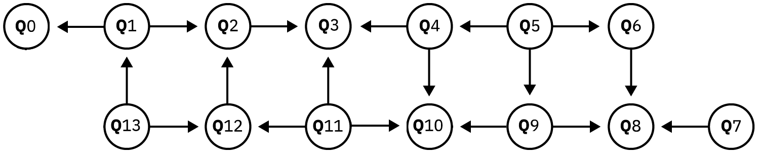
(d)   Melbourne

Figure 4.3: IBM quantum chips. Arrows between qubits indicate the directionality of CNOT gates: control $\rightarrow$ target. (Image source: QISKit Github https://github.com/Qiskit/ with modifications in Melbourne caption).

Since 2016, IBM company is providing universal quantum computer prototypes based on superconducting transmon qubits which are accessible on the cloud, both interactively in their web page, the Quantum Composer, and using a software development kit called QISKit.

Currently, there are four quantum devices available: two 5-qubit chips, Tenerife [Tenerife] and Yorktown [Yorktown], a 16-qubit chip, Rueschlikon [Rueschlikon] and a 14-qubit chip, Melbourne [Melbourne]. These devices are in their first version now, in 2019, but, except Melbourne, they are actually a second generation of the first prototypes: ibmqx2, ibmqx4 and ibmqx3/ibmqx5 respectively.

All backends work with a universal gate set composed by one-qubit unitary gate $U_{3}$ and a two-qubit gate, the CNOT gate. More information about quantum gates can be found in the App. LABEL:app:quantum_gates. Other basic gates are also configured in their low level quantum language, QISKit Terra, such as SWAP, $S$ or $H$ gates. However, it is important to keep in mind which is the basic gate set, as all other quantum gates will be decomposed in terms of the basic set automatically when the circuit is run, increasing the expected circuit depth.

The differences between devices, apart from the number of qubits, come from the qubits connectivity and the role that each qubit plays when a CNOT gate is applied: control or target. Figure 4.3 shows the connectivity of the available devices. Each qubit in the 5-qubit devices is connected with another two except the central one which is connected with the other four. Qubits in the 16-qubit and 14-qubit devices are connected with three neighbours in a ladder-type geometry. The one-directionality of the CNOT gate and the qubits connectivity are crucial for the quantum circuit implementation. If the circuit demands interaction between qubits that are not physically connected, we should implement SWAP gates which will increase our circuit depth and the probability of errors in our final result. Moreover, each time we need to implement a CNOT gate using as a control qubit a physical qubit which is actually a target, we have to invert the CNOT direction using Hadamard gates which, again, will increase the circuit depth and the error probability.

For our propose, Rueschnikon and Melbourne are the best choices for the implementation of the $n=4$ circuit. We can use any of the squares and identify upper qubits as 0 and 2 and lower qubits as 1 and 3, according to the circuit of Fig. LABEL:Fig:circuit.

4.5.2 Rigetti Computing: Forest

At the end of 2017, Rigetti Computing launched a 19-qubit processor, Acorn [Acorn], that can be used in the cloud through a development environment called Forest [Rigetti]. Forest includes a python toolkit, pyQuil, that allows the users to program, simulate and run quantum algorithms similar to IBM’s QISKit. The chip is made of 20 superconducting transmon qubits but, for some technical reasons, qubit 3 is off-line and cannot interact with its neighbors, so it is actually a 19-qubit device. In June 2018, they launched a new chip, Agave [Agave], made up of 8 qubits and recently, in November 2018, another chip of 16 qubits, Aspen-1.

Rigetti’s basic gate set is formed by three one-qubit rotational gates, $R_{z}(-\phi)$ and $R_{x}(\pm\pi/2)$ and a two-qubit gate, CZ. The minus sign added in the angle of $R_{z}$ gate is because Rigetti defines rotational gates as $e^{-i\frac{\theta}{2}\sigma_{i}}$ in contrast with the definition used in this thesis, $e^{i\frac{\theta}{2}\sigma_{i}}$. The use of the CZ gate instead of CNOT has the advantage of bi-directionality, as the result is the same independently of which is the control qubit. For that reason, the connectivity of the devices shown in Fig. 4.4 does not specify the direction of the two-qubit gate.

The qubit topology is very different from IBM’s devices. In Acorn chip, qubits are connected following a zigzag-type geometry, in Agave, qubits form a rectangle and in Aspen-1 they are located in two rings of 8 qubits each that are joined with two connections. Then, for the circuit of $n=4$ spins, we can not do without the fSWAP gates, which means that the circuit depth will be greater than the 16-qubits and 14-qubits IBM devices. On the other hand, it will be comparable with the 5-qubits devices, which also needs from these gates.

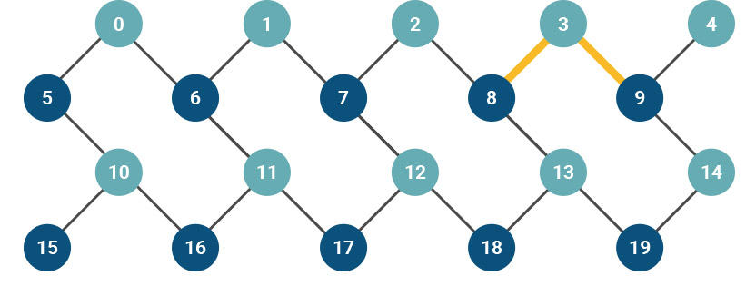
(a)   Acorn

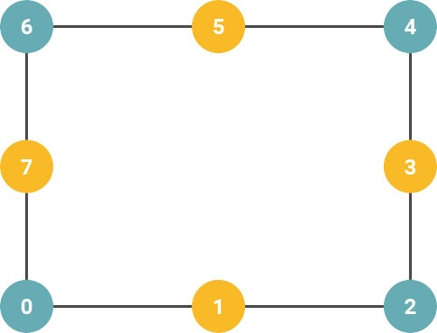
(b)   Agave

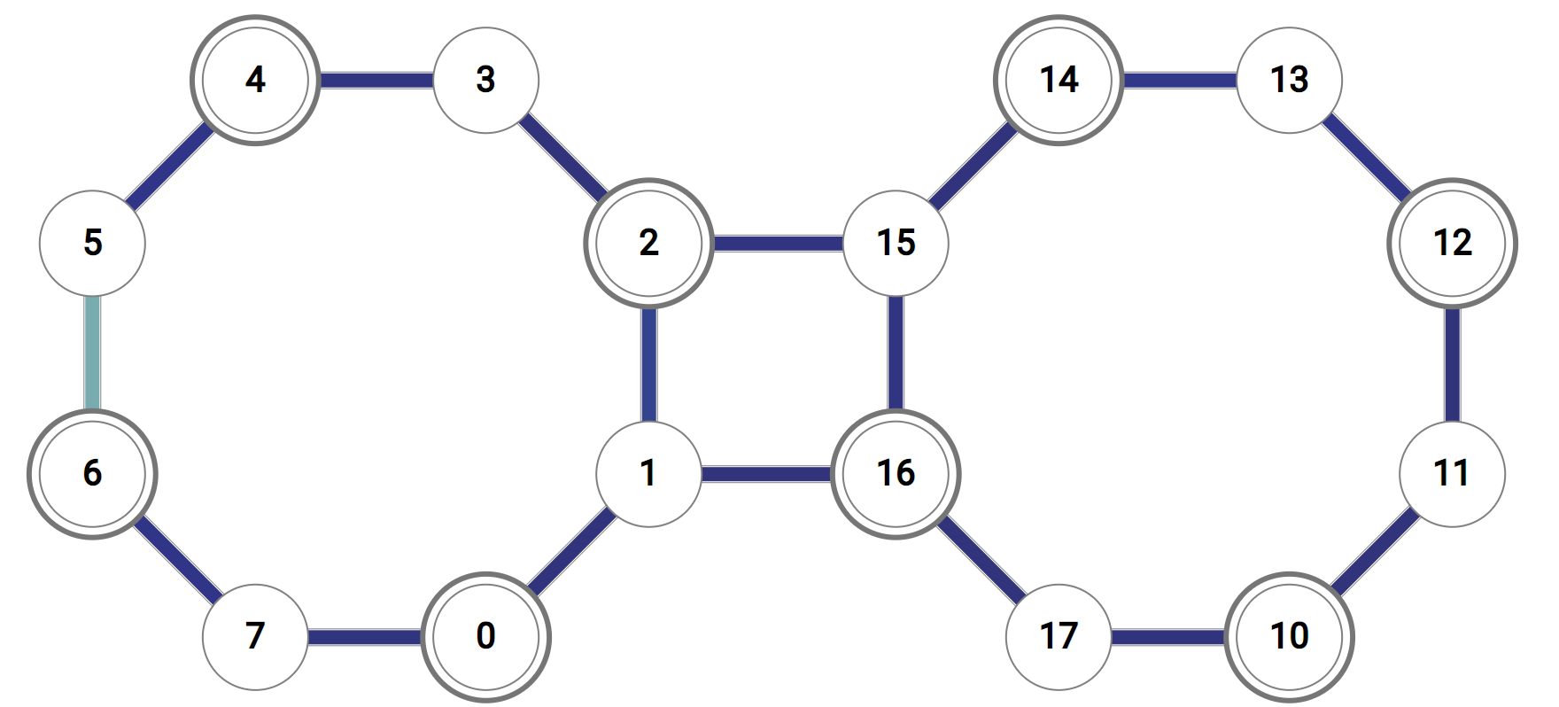
(c)   Aspen-1

Figure 4.4: Rigetti quantum chips architecture (Image source: Rigetti Computing web page https://www.rigetti.com/).

4.6 Results

The experimental results presented below were taken in a period between March and May 2018 in ibmqx4 (now Yorktown), ibmqx5 (now Rueschlikon) and Acorn devices. They were published in Ref. [Cervera18] and the program used for IBM devices was awarded and now is used as a tutorial [IBMtutorial]. Some properties and, specially, post-processing tasks offered by these two companies have changed recently, so the results if the circuits are run at the present moment could be different from the ones obtained.

Let’s set a particular case of the $XY$ model, the anti-ferromagnetic Ising spin chain, to do the experiments and to compare the performance of the three devices. Figure 4.5 shows the results of the exact simulation of ground state transverse magnetization. All points contain a statistical error of $1/\sqrt{N}$ with $N=1024$ which comes from the average over all runs to compute the expected value. The other error sources are discussed qualitatively in the following paragraphs.

The best performance comes from the ibmqx5 device. This is an expected result as we do not need from fSWAP gates because the qubits connectivity. On the other hand, Rigetti’s device, Acorn, perform better than the ibmqx4, even though the number of gates is very similar. Again, it is important to point out that these results could change if we run the experiment at present. In fact, the results obtained after running a quantum circuit could differ depending on the time of the day that they were taken. Each quantum device is calibrated every few hour so the results are expected to be better immediately after this calibration rather than hours later.

The simulation approaches better to the prediction for low $\lambda$. The explanation could come from how affect the experimental error sources to the magnetization. Assuming that two-qubit gates implementation take several hundreds of ns and single qubit gates around one hundred of ns, errors coming from decoherence are expected to be low, as these times are around 50 $\mu$s. On the other hand, errors coming from the gate implementation are cumulative and probably the most important error source. It is not negligible neither errors coming from qubits readout, which can induce a bit flip.

The analysis of the results become more clear if we look at the exact ground state wave function:

$$|gs\rangle=\frac{1}{\mathcal{N}}\left\{\begin{array}[]{ll}\sqrt{2}\alpha\left(|00\rangle|\Psi^{-}\rangle+|\Psi^{-}\rangle|00\rangle\right)+|11\rangle|\Psi^{-}\rangle+|\Psi^{-}\rangle|11\rangle&\mathrm{for}\ \lambda<1,\\ \alpha\left(|0011\rangle-|0110\rangle+|1001\rangle+|1100\rangle\right)+2|1111\rangle&\mathrm{for}\ \lambda>1,\end{array}\right.$$ (4.37)

where $\alpha=\lambda-\sqrt{1+\lambda^{2}}$, $\mathcal{N}=2\sqrt{2}\sqrt{1+\lambda\alpha}$ and $|\Psi^{-}\rangle=(|01\rangle-|10\rangle)/\sqrt{2}$. As $\lambda$ increases, the amplitude for the states proportional to $\alpha$ goes to zero. That means that any error occurring for $\lambda>1$ is dramatic as it will affect the state with higher probability amplitude, the $|1111\rangle$. Then, any error in that regime will inevitably cause a decrease in magnetization. On the other hand, errors in some states for $\lambda<1$ can be compensated in average for the other elements with the same probability amplitude.

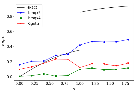
Figure 4.5: Expected value of $\langle\sigma_{z}\rangle$ of the ground state of an $n=4$ Ising spin chain as a function of transverse field strength $\lambda$. Solid line represents the exact result in comparison with the experimental simulations represented by scatter points. The best simulation comes from ibmqx5 device, which is an expected result since the number of gates used is lesser than with the other devices because of qubits connectivity.

Similar results are obtained for the time evolution simulation. Figure 4.6 shows the results for the simulation of the $|\uparrow\uparrow\uparrow\uparrow\rangle$ state transverse magnetization as it was explained in Sec. 4.3. As for the preparation of the initial state it is necessary to implement more gates, only the results for the ibmqx5 device are shown, which is the one that could afford this extra circuit depth.

As expected from the previous result, points that represent higher magnetization carry more errors respect to the predicted theoretical values. However, it is remarkable that the relations among the different points along the values of transverse magnetic field are proportionally correct. The oscillations take place for lower values of $\langle\sigma_{z}\rangle$, have lower amplitudes and are a little bit shifted to the left. Even though, they cross each other at the corresponding points and increase and decrease proportionally to the exact result. That is a clear indicator that the error sources in the quantum device are systematic, as the result does not depend on the state preparation.

As a final remark, notice that we compute the transverse magnetization instead of the staggered magnetization, i.e. $M_{x}=\sum_{i}(-1)^{i}\sigma^{x}_{i}$, which is the order parameter for the anti-ferromagnetic Ising model. For the purpose of these experiments, it is more natural to compute $\langle\sigma_{z}\rangle$, since the states obtained with these quantum devices are expressed in the $\sigma_{z}$ basis. However, it will be straightforward to compute $M_{x}$ as the only change needed appears in the classical post-processing part.

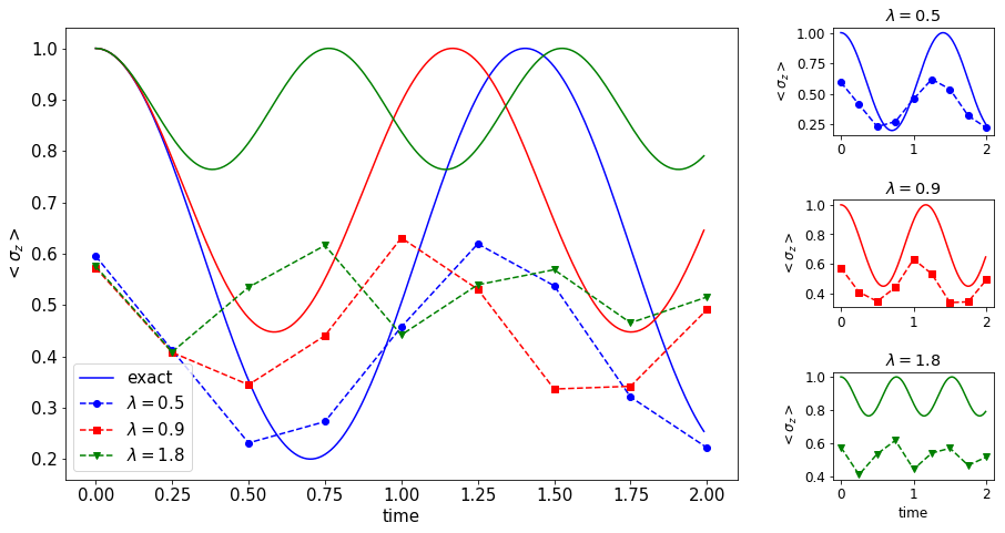
Figure 4.6: Time evolution simulation of transverse magnetization, $\langle\sigma_{z}\rangle$, for the state $|\uparrow\uparrow\uparrow\uparrow\rangle$ of an $n=4$ Ising spin chain. Left plot compares the exact result with the experimental run in the ibmqx5 chip for different values of $\lambda$. Right plots detailed the results for each $\lambda$ to compare them with the theoretical values. Although the magnetization is lesser than expected, the oscillations follow the same theoretical pattern.

4.7 Conclusions

In this chapter, it has been implemented the exact simulation of a one-dimensional Ising spin chain with a transverse field in some quantum computer prototypes: two from IBM and one from Rigetti computing. The method to construct a quantum operation that diagonalize exactly the $XY$ Hamiltonian has been reviewed, providing the explicit circuit for the simulation of an $n=4$ spin chain. It has been also introduced novel approaches to simulate time and thermal evolution using the circuit obtained, in particular, to compute the ground state transverse magnetization and the time evolution of the state of all spins aligned.

The circuit presented allows computing all eigenstates of the $XY$ Hamiltonian by just initializing the qubits in one of the states of the computational basis. It is then an implementation of a Slater determinant with a quantum computer. Because of the one-dimensional $XY$ model is an exactly solvable model, which means that we can compute analytically all the states and energies for any number of spins, and the circuit is efficient, the number of gates scales as $n^{2}$ and the circuit depth as $n\log n$, it can represent a method to test quantum computing devices of any size. As has been shown, it is also a hard test because the simulation of the phase transition surrounding and time evolution require a high qubits control.

The best performance has been obtained with the ibmqx5 chip, although the error respect to the theoretical prediction is large in the paramagnetic phase of the model. A possible reason why this chip shows better results than the others comes from the number of gates used in the quantum circuit, as the qubits connectivity in that device allows us to save all the fSWAP gates. On the other hand, Rigetti’s chip performs better than the ibmqx4 chip, even though both implemented circuits have the same gate depth. However, the results of these few qubits experiments could change totally if we run the circuits again. The results shown were obtained a few months before this thesis was written and, from then on, the quantum devices have changed their properties. In conclusion, this work represents just a proof of concept of how quantum computers can be tested and compared.

The paramagnetic phase is difficult to simulate due to the fact that any error that can induce a qubit bit flip will produce a decrease in magnetization, as can be traced out from the ground state wave function of Eq. (4.37). However, and taking into account this fact, the time evolution simulation is reasonably good, as the expected oscillations for different transverse magnetic field strengths are shifted to the left and have lower amplitude and magnetization, but are also proportional to each other as are the theoretical values.

As a final remark, this circuit is also interesting from a point of view of condensed matter physics as specific methods to simulate exactly time and thermal evolution are provided. This can open the possibility of simulating other interesting models: integrable, like Kitaev Honeycomb model [Schmoll17], or with an ansatz, like the Heisenberg model [Bethe31].

Chapter 5 Absolute Maximal Entanglement in Quantum Computation

La mode est architecture: c’est une question de proportions.

–Coco Chanel

The proliferation of quantum computing devices has caused the necessity of benchmark methods to test them. Current quantum computers are typically characterized by its number of qubits and its connectivity and its performance is measured with gate fidelities, coherence and relaxation times. However, the results obtained are far below the expected accuracy if errors of gates were to be taken at face value and considered independent, as has been already shown in the results of the previous chapter.

Several proposals exist to benchmark quantum computers. As an example, corporations like IBM have defined a figure of merit called quantum volume to quantify the quality of their devices [Volume]. This method follows the ideas of randomize benchmarking [Knill08], another method used to extract qubit gate fidelities. In the previous chapter, we have introduced the simulation of exactly solvable models in a quantum computer, which can be also used as a benchmark method since we can compare the result obtained with the correct solution computed analytically. However, all these methods do not take into account the probably principal resource of quantum computation: entanglement. Although one expects to develop some amount of entanglement in the protocols presented above, are quantum computers able to generate as much entanglement as we will require? The only way to test it is by forcing quantum devices to generate highly entangled states and observe if they are capable to support them.

We know that entanglement is at the core of quantum advantage. Or, in other words, quantum advantage is a consequence of high entanglement generation. This is not surprising since Bell inequalities are violated by high entangled states: quantum physics cannot be described classically because of the existence of entanglement.

In this chapter, we present some quantum circuits that generate Absolutely Maximally Entangled (AME) states, i.e. states that maximally entangle all their bipartitions. The circuits introduced are composed by few CZ gates and one-qubit gates that can be performed in parallel. This proposal is distinctly different from bosonic sampling [Aaronson13], where large entanglement is developed along the circuit to make it impossible to be faithfully reproduced by classical simulation. In a sense, maximally entangled states are a test for a useful quantum computer, not for quantum advantage.

The existence of this kind of states is limited: for qubits, they only exist for $n=2,3,5$ and 6 parties. For that reason, we also propose to simulate AME states of higher dimensions using qubits. The results will maximally entangle some parties although not of them. We derive some interesting properties of these circuits, for example, that the entropy is majorized after each entangling gate is applied. This characteristic could be a consequence of circuit optimality.

Beside benchmarking interest, AME states define an interesting mathematical problem itself and attractive practical applications. These include quantum secret sharing [Helwig12, HC13], open destination quantum teleportation [HC13] and quantum error correcting codes [Scott04]. The last one is a fundamental ingredient for building a quantum computer. In addition, there is a natural link between AME states and holography through error correcting codes [Latorre15, Pastawski15].

The structure of this chapter is organized as follows. First, we introduce a short review of AME states that includes its definition and the most fundamental properties. Second, in Sec. LABEL:sec:graph, we present the graph state formulation that we will use to construct the quantum circuits for AME states. These circuits are shown in Sec. LABEL:sec:AMEgraph and the simulation of AME states of $d>2$ with qubits in Sec. LABEL:sec:AMEqubits. For its interest in error correcting codes, we present an example of an AME state of minimal support in Sec. LABEL:sec:AMEminimal. Finally, we introduce the entropy majorization analysis in Sec. LABEL:sec:maj and close with the conclusions in Sec. LABEL:sec:AMEcon.

5.1 Absolutely Maximally Entangled states

The formal definition of an Absolutely Maximally Entangled (AME) state is the following:

Definition 5.1.1 — Absolutely Maximally Entangled states. 

An AME($n,d$) state is a $n$ qudit state with local dimension $d$ whose all possible bipartitions to $\lfloor n/2\rfloor$ parties are maximally entangled, i.e. all reduced density matrices are proportional to the identity.

Such states are maximally entangled when considering the entropy of reductions as a measure of multipartite entanglement. Thus, all bipartitions of an AME state have entropy

$$S=\left\lfloor\frac{n}{2}\right\rfloor\ ,$$ (5.1)

taking the $\log$ in $d$ basis.

Bell states and GHZ state are AME states for the bipartite and tripartite cases respectively and for any dimension $d$. However, the GHZ states for $n\geq 4$ are not AME states. The existence of AME($n,d$) states $\forall\ n$ and $d$ is a hard open problem. Only for qubits, $d=2$, the problem is fully solved: an AME($n$,2) exist only for $n=2,3,5,6$ [Helwig13, Huber16].

AME states connect to different mathematical ideas. One example is the family of AME states of minimal support which are one-to-one related to a special class of maximum distance separable codes [Huffman03, MDS], index unity orthogonal arrays [Goyeneche14, Seveso18], permutation multi-unitary matrices when $n$ is even [Goyeneche15] and to a set of $m=n-\lfloor n/2\rfloor$ mutually orthogonal Latin hypercubes of size $d$ defined in dimension $\lfloor n/2\rfloor$ [Goyeneche18].