A study of a nonlocal problem with Robin boundary conditions arising from MEMS technology

Abstract.

In the current work we study a nonlocal parabolic problem with Robin boundary conditions. The problem arises from the study of an idealized electrically actuated MEMS (Micro-Electro-Mechanical System) device, when the ends of the device are attached or pinned to a cantilever. Initially the steady-state problem is investigated estimates of the pull-in voltage are derived. In particular, a Pohožaev’s type identity is also obtained which then facilitates the derivation of an estimate of the pull-in voltage for radially symmetric $N-$dimensional domains. Next a detailed study of the time-dependent problem is delivered and global-in-time as well as quenching results are obtained for generic and radially symmetric domains. The current work closes with a numerical investigation of the presented nonlocal model via an adaptive numerical method. Various numerical experiments are presented, verifying the previously derived analytical results as well as providing new insights on the qualitative behaviour of the studied nonlocal model.

1. Introduction

In this work we study the following nonlocal parabolic problem:

$$u_{t}=\Delta u+\frac{\lambda}{\left(1-u\right)^{2}\left[1+\alpha\int_{\Omega}1/(1-u\,)dx\right]^{2}},\quad\quad\mbox{in}\quad Q_{T}:={\Omega}\times(0,T),\;T>0,$$ (1.1a)

$$\frac{\partial u}{\partial\nu}+\beta u=0,\quad\mbox{on}\quad\Gamma_{T}:={\partial}{\Omega}\times(0,T),$$ (1.1b)

$$u(x,0)=u_{0}(x),\quad x\in\Omega,$$ (1.1c)

where $\lambda>0$, $\alpha>0$, $\beta>0$, are given positive constants. Especially, ${\lambda}$ is proportional to the applied voltage into the system, called pull-in voltage parameter, and it is actually the controlling parameter for the operation of the considered MEMS device. The initial data $u_{0}(x)$ is assumed to be a smooth function such that $0<u_{0}(x)<1$ for all $x\in\bar{\Omega}$ and $\frac{\partial u_{0}}{\partial\nu}+\beta u_{0}=0,\;\;\mbox{for}\;\;x\in\ \partial\Omega;$ here $\nu=\nu(x)$ stands for the unit outward normal vector on the boundary of the $N-$dimensional domain ${\Omega}.$ Notably, from the applications point of view only the cases $N=1,2$ are viable, however from the point of view of mathematical analysis cases $N\geq 3$ are also interesting and so they will be investigated. Moreover, here $T$ denotes the maximum existence time of solution $u.$

When $\alpha=0$ problem (1.1) reduces to the local parabolic problem

$$u_{t}=\Delta u+\frac{\lambda}{(1-u)^{2}},\quad\mbox{in}\quad Q_{T},$$ (1.2a)

$$\frac{\partial u}{\partial\nu}+\beta u=0,\quad\mbox{on}\quad\Gamma_{T},$$ (1.2b)

$$u(x,0)=u_{0}(x),\quad x\in\Omega.$$ (1.2c)

It is worth mentioning that for Robin type boundary conditions, as the ones considered above for $\beta>0,$ there is a limited study for the local problem, cf. [15], while to the best of our knowledge no published works dealing with the nonlocal problem (1.1) can be found in the literature. Our motivation for studying (1.1) comes from the fact that it is actually linked with special applications in MEMS industry, as pointed below. Furthermore, due the imposed Robin-type boundary conditions extra technical difficulties arise compared to the study of the Dirichlet problem, a fact that is indicated through the manuscript.

Problem (1.1) arises as a mathematical model which describes the operation of some electrostatic actuated micro-electro-mechanical systems (MEMS). Those MEMS systems are precision devices which combine mechanical processes with electrical circuits. MEMS devices range in size from millimeters down to microns, and involve precision mechanical components that can be constructed using semiconductor manufacturing technologies.

In particular, electrostatic actuation is a popular application of MEMS. Various electrostatic actuated MEMS have been developed and used in a wide variety of devices applied as sensors and have fluid-mechanical, optical, radio frequency (RF), data-storage, and biotechnology applications. Examples of microdevices of this kind include microphones, temperature sensors, RF switches, resonators, accelerometers, micromirrors, micropumps, microvalves, etc., see for example [9, 38, 47].

In the sequel a derivation for the nonlocal model (1.1), for the one-dimensional case, is presented and also the association of that model with applications in MEMS industry is explained. The main body of the derivation is standard (see for example [28, 29, 32, 38]), however in order to justify the inclusion for the Robin boundary conditions in the model and for completeness it is presented here as well. The modifications of this modelling approach are presented in detail in the next section.

1.1. Derivation of the model

We consider an idealized electrostatiaclly MEMS device which consists of an elastic membrane and a rigid plate placed parallel to each other as it can be seen in Figure 1. The membrane has two parallel sides usually attached or pinned to a cantilever, while the other sides are free. Both membrane and plate have width $w$ and length L, and in the undeformed state (for the membrane) the distance between the membrane and the plate is $l.$ We assume here that the gap between the plate and the membrane is small, that is $l\ll L$ and $l\ll w.$ Besides, the area between the elastic mebrane and the rigid plate is occupied by some inviscid material with dielectric constant one, so permittivity is that of free space, $\epsilon_{0}$.

Figure 1. Schematic representation of a MEMS device

A potential difference $V$ is applied between the top surface and the rigid plate and we further assume that the plate is earthed. Besides, the small aspect ratio of the gap gives potential

$$\phi=V(l-z^{\prime})/(l-u^{\prime}),$$ (1.3)

to leading order, where $u^{\prime}$ is the displacement of the membrane towards the plate ($u^{\prime}=l$ corresponds to touch-down, i.e. when the top surface touches the rigid plate) and $z^{\prime}$ is the distance measured from the undisturbed membrane position towards the plate. The electrostatic force per unit area on the membrane (in the $z^{\prime}$ direction) is then

$\frac{1}{2}\times\mbox{surface charge density}\times\mbox{electic field}=\frac{1}{2}\epsilon_{0}\phi_{z^{\prime}}^{2}=\frac{1}{2}\epsilon_{0}V^{2}/(l-u^{\prime})^{2}\,,$

recalling that $\epsilon_{0}$ is the permittivity of the free space.

We take the sides of width $w$, say at $x^{\prime}=0$ and $x^{\prime}=L$, to be connected with the support of the device, with those of length $L$, say at $y^{\prime}=0$ and $y^{\prime}=w$, to be free. We also assume there is no variation in the $y^{\prime}$ direction, so $u^{\prime}=u^{\prime}(x^{\prime},z^{\prime},t^{\prime})$ for time $t^{\prime}.$ The surface density of the membrane is denoted by $\rho$, while $T_{m}$ stands for constant surface tension of the membrane. Then its displacement satisfies the forced wave equation with damping (proportional to the membrane speed),

$$\rho u^{\prime}_{t^{\prime}t^{\prime}}+au^{\prime}_{t^{\prime}}=T_{m}u^{\prime}_{x^{\prime}x^{\prime}}+\frac{1}{2}\epsilon_{0}V^{2}/(l-u^{\prime})^{2}.$$ (1.4)

In many situations is observed that the damping term is dominant compared with the inertia term. According to this ansatz we get the following parabolic equation

$$au^{\prime}_{t^{\prime}}=T_{m}u^{\prime}_{x^{\prime}x^{\prime}}+\frac{1}{2}\epsilon_{0}V^{2}/(l-u^{\prime})^{2}.$$ (1.5)

In addition to the derived equation (1.5), appropriate boundary conditions should be imposed. The standard way to do so is to assume that since the edges of the membrane or beam are fixed at the support of the device, Dirichlet boundary conditions, in the case of the flexible membrane or clamped boundary conditions, in the case of a beam should be considered. Although as it is stated in [47, Chapter 6] it is evident that the support or cantilever of MEMS devises might be nonideal and flexible.

More specifically cantilever microbeams can tilt upward or downward due to the deformation of their support since the anchors or supports of them can have some flexibility making the assumption of perfect clamping inaccurate. This flexibility of the supports of microbeams are accounted for by assuming springs at the beam boundaries and consequently modeling a flexible nonideal support can be done in general by assuming torsional and translational springs at the membrane or beam edge.

As a first step towards this modelling approach in this work we will assume that we have a device for which its movable upper part is thin enough, so that it can be considered to behave as a membrane while its ends are connected with a flexible nonideal support behaving as a spring moving in the $x^{\prime}$-direction, see Figure 2(a). Torsional or other kind of behaviour is assumed to be negligible at this occasion.

Therefore according to the above assumptions the appropriate boundary conditions should be those of Robin type and thus we set

$$u^{\prime}_{x^{\prime}}(-L,t^{\prime})=ku^{\prime}(-L,t^{\prime}),\quad u^{\prime}_{x^{\prime}}(L,t^{\prime})=-ku^{\prime}(L,t^{\prime}),$$

where $k$ is the spring constant.

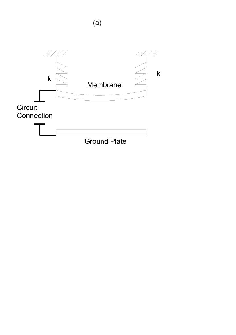
Figure 2. (a) Schematic representation of a MEMS device with nonideal support. (b) Schematic representation of a MEMS device with radial symmetry

Next by introducing the scaling $u^{\prime}=lu$, $x^{\prime}=Lx$, $t^{\prime}=\frac{L^{2}a}{T_{m}}t$, we end up with the local equation

$$u_{t}=u_{xx}+(\epsilon_{0}V^{2}L^{2}/T_{m}{2l^{3}})/(1-u)^{2},$$ (1.6)

associated with the aforementioned boundary conditions and some appropriate initial deformation $0<u(x,0)<1.$ Therefore we end up in the first place with the following local problem:

$$u_{t}=u_{xx}+\frac{\lambda}{\left(1-u\right){{}^{2}}},\quad-1<x<1,\quad t>0,$$ (1.7a)

$$u_{x}(\mp 1,t)=\pm\beta u(\mp 1,t),\quad t>0,$$ (1.7b)

$$u(x,0)=u_{0}(x),\quad-1<x<1,$$ (1.7c)

for $\beta=Lk$ and $\lambda=\frac{\epsilon_{0}V^{2}L^{2}}{T_{m}{2l^{3}}}.$

Since pull-in instability is a ubiquitous feature of electrostatically actuated systems, many researchers have focused on extending the stable operation of electrostatically actuated systems beyond the pull-in regime. In particular, in [44, 45] the basic capacitive control scheme was first proposed by Seeger and Crary to elaborate this kind of stabilization, see also [6]. More precisely, this scheme provides control of the voltage by the addition of a series capacitance to the circuit containing the MEMS device, since the added capacitance acts as a voltage divider. So in the event the MEMS device, which has a capacitance $C$ depending on displacement, is connected in series with a capacitor of fixed capacitance $C_{f}$ and a source of fixed voltage $V_{s}$, we have that

$$V_{s}=\frac{Q}{C_{c}}=Q\left(\frac{1}{C}+\frac{1}{C_{f}}\right),$$

where $Q$ is the charge on the device and fixed capacitor, and $C_{c}$ the series capacitance of the two. Then the potential difference $V$ across the MEMS device, by applying Kirchoff’s law is equal to

$$V=\frac{V_{s}}{1+C/C_{f}}.$$ (1.8)

In addition we also have

$$Q=\epsilon_{0}\int_{0}^{w}\int_{0}^{L}\phi_{z^{\prime}}(x,y,0)\,dx^{\prime}\,dy^{\prime}=V\frac{wL\epsilon_{0}}{l}\int_{0}^{1}\frac{1}{1-u}\,dx\,,$$

and by using relation (1.3) we get,

$$C=C_{0}\int_{0}^{1}\frac{1}{1-u}\,dx,$$

for $C_{0}=\frac{wL\epsilon_{0}}{l}$ being the capacitance of the undeflected device.

When the latter relation is combined with equations (1.8) and (1.6) we finally obtain the nonlocal problem

$$u_{t}=u_{xx}+\frac{\lambda}{(1-u)^{2}\left(1+\alpha\int_{-1}^{1}\frac{1}{1-u}\,dx\right)^{2}},\;-1<x<1,\quad t>0,$$ (1.9a)

$$u_{x}(\mp 1,t)=\pm\beta u(\mp 1,t),\quad t>0,$$ (1.9b)

$$u(x,0)=u_{0}(x),\quad-1<x<1,$$ (1.9c)

with $\alpha=\frac{wL\epsilon_{0}}{lC_{f}}=\frac{C_{0}}{C_{f}}$.

Usually it is supposed that the elastic membrane is initially in its unforced position , so that $u(x,0)\equiv 0.$ However, in this work, we consider more general non-negative initial conditions, reflecting also the situation when the membrane has an initial displacement.

It has been experimentally observed that the applied voltage $V_{s}$ controls the operation of the MEMS device. Indeed, when $V_{s}$ exceeds a critical threshold $V_{cr}$, called the pull-in voltage, then the phenomenon of touch-down (or pull-in instability as it is also known in MEMS literature) occurs when the elastic membrane touches the rigid ground plate. The related mathematical problem has been studied quite extensively in e.g. [9, 21, 22, 27, 29, 32, 35, 40, 41].

Note that the limiting case $\alpha=0$ corresponds to the configuration where there is no capacitor in the circuit and then we end up with the local problem (1.7), which has been studied in [15]. A stochastic version of problem (1.7) is treated in [7, 31]. Besides, the local problem with Dirichlet boundary conditions ($\beta=+\infty$) has been extensively studied among others in [9, 21, 27, 32]. Also, for hyperbolic modifications of the variation of (1.7) an interested reader can check [14, 29].

The quenching behaviour of the nonlocal equation (1.1a) associated with Dirichlet boundary ($\beta=+\infty$) has been treated in [30] and in references therein as well as in [18, 19, 23]. Also, non-local alterations of parabolic and hyperbolic problems arising in MEMS technology were tackled in [8, 18, 20, 19, 28, 30, 32]. However to the best of our knowledge there are not similar studies available in the literature for the Robin problem ($0<\beta<+\infty,$) so in the current work we study problem (1.1) and we extend some of the results given in [15] for the local problem, but we also deliver a further investigation related to the steady-state problem and the quenching behaviour of the time-dependent problem. Our mathematical analysis is inspired by ideas developed in [19, 30], however important modifications are necessary due to the Robin boundary conditions. In particular, a new Pohožaev’s type identity for Robin boundary conditions is derived which is then used to derive lower estimates of the pull-in voltage. Moreover, a novel argument, see Theorem 3.15, is developed to derive an upper estimate of the quenching rate; note that such a reasoning is missing from the approach used in [30]. Still, the derivation of a key estimate for the nonlocal term, analogous to the one derived in [30, Lemma 3.3 ] for the Dirichlet problem, needs more work for Robin problem (1.1) and it is finally derived under some extra restriction, cf. Lemma 3.10.

The organization of the paper is as follows. In section 2 a thorough study of the steady-state problem is delivered, where among other results some estimates of the supremum of its spectrum (pull-in voltage) are derived. Uniqueness and local-in-time existence results for time-dependent problem (1.1) are discussed in the first part of section 3. The second part of section 3 deals with the long-time behaviour of the solutions of (1.1). In particular, at first a quenching result is obtained for a genericl domain, whilst a sharper quenching result is derived for a radially symmetric domain later on. A numerical treatment of (1.1) via an adaptive method is presented in section 4. We thus numerically verify all the obtained analytical results as well as we determine the quenching profile which cannot be derived via our theoretical approach. We conclude with a discussion of our main results in section  5.

2. Steady-State Problem: estimates of the pull-in voltage

The main purpose of the current section is to study the steady-state problem of (1.1). In particular, we are interested in obtaining estimates of the supremum of its spectrum (pull-in voltage) whilst in the one-dimensional case we are also able to derive the form of its bifurcation diagram.

2.1. The one-dimensional case

Below we provide a thorough investigation of the steady-state problem in the one-dimensional case. In particular we study the structure of the solution set of

$$w^{\prime\prime}+\frac{{\lambda}}{(1-w)^{2}\left[1+\alpha\int_{-1}^{1}\frac{{\mathrm{d}}x}{1-w}\right]^{2}}=0,\;\;-1<x<1,$$ (2.1a)

$$w^{\prime}(-1)-\beta w(-1)=0,\quad w^{\prime}(1)+\beta w(1)=0,$$ (2.1b)

where we always have $0\leq w<1$ in $[-1,\,1]$ for a (classical) solution of (2.1).

For convenience we set $W=1-w$ and then (2.1) becomes

$$W^{\prime\prime}=\frac{\mu}{W^{2}}\,,\quad-1<x<1,$$ (2.2a)

$$W^{\prime}(-1)+\beta\left(1-W(-1)\right)=0\,,\quad W^{\prime}(1)-\beta\left(1-W(1)\right)=0\,,$$ (2.2b)

where

$$\mu=\frac{\lambda}{\left[1+\alpha\int_{-1}^{1}\frac{1}{W}dx\right]^{2}}.$$ (2.3)

Note that $W$ is symmetric and thus $m=\min\{W(x),x\in[-1.1]\}=W(0)$, cf. [13, 20]. Then multiplying both sides of equation (2.2a) by $W^{\prime}$ and integrating from $m=W(0)$ to $W(x)=W$ we derive

$$\int_{0}^{W^{\prime}}W^{\prime}dW^{\prime}=\int_{0}^{x}W^{\prime\prime}W^{\prime}dx=\mu\int_{0}^{x}\frac{W^{\prime}}{W^{2}}\,dx=\mu\int_{m}^{W}\frac{dW}{W^{2}}\,,$$

hence

$$\frac{1}{2}{(W^{\prime})}^{2}=\mu\left(\frac{1}{m}-\frac{1}{W}\right).$$ (2.4)

This gives equivalently

$$\frac{dx}{dW}=\sqrt{\frac{m}{2\mu}}\sqrt{\frac{W}{W-m}}\,,$$ (2.5)

which implies (see  [20, 28])

$$x=\sqrt{\frac{m}{2\mu}}\left[\sqrt{W(W-m)}-\frac{1}{2}m\ln(m)+m\ln\left(\sqrt{W}+\sqrt{W-m}\right)\right]\,.$$

Additionally at the point $x=1$ and for $W(1)=M:=\max\{W(x),\;x\in[-1,1]\}$ we deduce

$$1=\sqrt{\frac{m}{2\mu}}\left[\sqrt{M(M-m)}-\frac{1}{2}m\ln(m)+m\ln\left(\sqrt{M}+\sqrt{M-m}\right)\right]\,.$$ (2.6)

Moreover combining the boundary condition, $W^{\prime}(1)=\beta\left(1-W(1)\right)$, with equation (2.4) we obtain

$$\frac{\beta^{2}(1-M)^{2}}{2}=\mu\left(\frac{1}{m}-\frac{1}{M}\right).$$ (2.7)

At this point, recalling that for $\alpha=0$ we have $\mu=\lambda,$ we can obtain the bifurcation diagram of the local problem. More specifically rearranging (2.7), we have

$$m=\frac{2\lambda M}{2\lambda+M\beta^{2}(1-M)^{2}},$$ (2.8)

which together with (2.6), for $\mu=\lambda$, namely

$$1=\sqrt{\frac{m}{2\lambda}}\left[\sqrt{M(M-m)}-\frac{1}{2}m\ln(m)+m\ln\left(\sqrt{M}+\sqrt{M-m}\right)\right],$$ (2.9)

forms a system of algebraic equations giving an implicit relation of the form $F(\lambda,M)=0$.

Furthermore in order to obtain the bifurcation diagram for the nonlocal problem ($\alpha>0$) we have to express the integral of the nonlocal term in terms of $\lambda,m,M$.

That is, on using equation (2.5)

$$\int_{-1}^{1}\frac{1}{W}dx=\int_{-1}^{1}\frac{dx}{dW}\frac{dW}{W}=2\sqrt{\frac{m}{2\mu}}\int_{m}^{M}\frac{1}{\sqrt{W(W-m)}}dW$$

$$= 2\frac{1}{\sqrt{M(M-m)}-\frac{1}{2}m\ln(m)+m\ln\left(\sqrt{M}+\sqrt{M-m}\right)}\int_{m}^{1}\frac{1}{\sqrt{W(W-m)}}dW$$

$$= 2\frac{1}{\sqrt{M(M-m)}-\frac{1}{2}m\ln(m)+m\ln\left(\sqrt{M}+\sqrt{M-m}\right)}\ln\left(\frac{2M-m+2\sqrt{M(M-m)}}{m}\right).$$

Therefore, using also (2.3), (2.7) to eliminate $\mu$, we obtain the following system of algebraic equations for $\lambda$, $M$, $m$:

$$1=\sqrt{\frac{m}{2\mu}}\left[\sqrt{M(M-m)}-\frac{1}{2}m\ln(m)+m\ln\left(\sqrt{M}+\sqrt{M-m}\right)\right],$$ (2.10a)

$$\frac{\beta^{2}(M-1)^{2}}{2}\frac{mM}{M-m}=\lambda{\left[1+\alpha\frac{2\ln\left(\frac{2M-m+2\sqrt{M(M-m)}}{m}\right)}{\sqrt{M(M-m)}-\frac{1}{2}m\ln(m)+m\ln\left(\sqrt{M}+\sqrt{M-m}\right)}\right]^{-2}},$$ (2.10b)

together with (2.3), which can be solved numerically.

Remark 2.1.

Note that by equation (2.7) for $\beta\gg 1$ we have $(M-1)\sim 0$ or $M\sim 1$ and we retrive the expression for $\lambda$ and $m$ which gives the bifurcation diagram for the local problem with Dirichlet boundary conditions (see [28] ), i.e.

$$\lambda=\frac{m}{2}\left[\sqrt{1-m}-\frac{1}{2}m\ln(m)+m\ln\left(1+\sqrt{1-m}\right)\right]^{2}.$$

In Figure 3(a) we plot the bifurcation diagram for the stationary local problem (2.1a) for $\alpha=0$. We can observe the existence of a critical value of the parameter $\lambda$, say $\lambda^{*},$ usually called the pull-in voltage in MEMS literature, above which we have no solution for the steady problem while for values below $\lambda^{*}$ we have two solutions. We finally derive that $\lambda^{*}=0.108711900526435$ and for this value we have that the maximum of the solution $M=W(1)=0.761$.

Regarding the nonlocal stationary problem, equation (2.1a) with $\alpha=1$ we present a similar plot of the bifurcation diagram in Figure 4(a) (line indicated with $\alpha=1$). In this case the critical value of the parameter $\lambda$ is $\lambda^{*}=2.387086785660011$. In both of the above cases the parameter in the boundary conditions is taken to be $\beta=1$.

In this set of graphs we can see also the variation of the bifurcation diagram of the local problem with respect to the parameter $\beta$ in Figure 3(b).

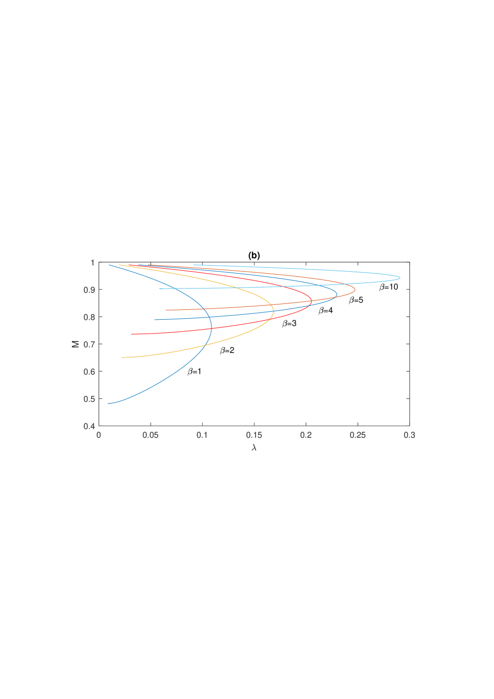
Figure 3. (a) Bifurcation diagram for the local problem. (b) Variation of the bifurcation diagramm of the local problem with respect to the parameter $\beta$.

A similar graph, see Figure 4, investigates the variation of the bifurcation diagram of the nonlocal problem with respect to the parameter $\alpha$ in Figure 4(a) and with respect to the parameter $\beta$ in Figure 4(b).

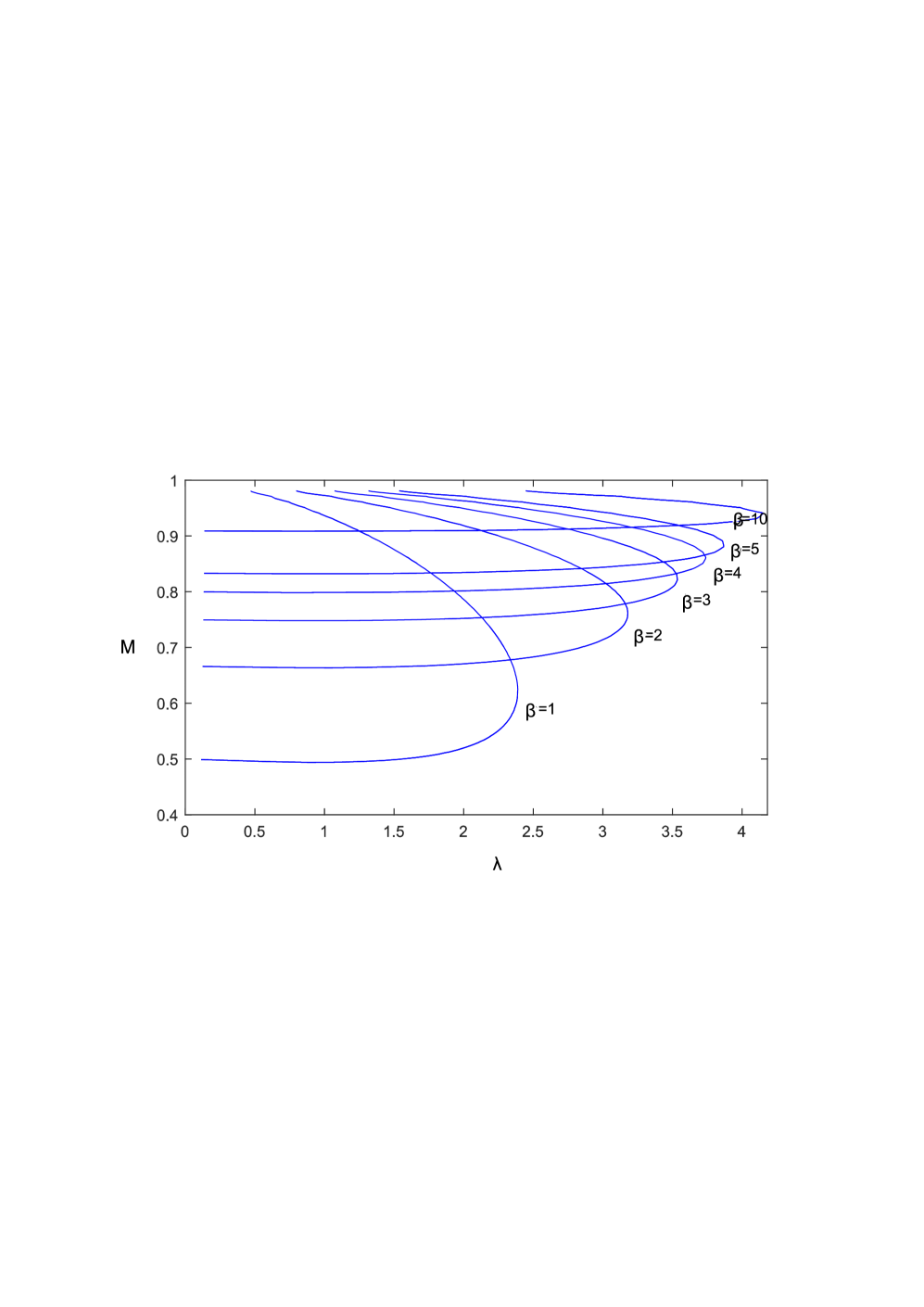
Figure 4. (a) Variation of the bifurcation diagramm of the nonlocal problem with respect to the parameter $\alpha$ for $\beta=1$. (b) Variation of the bifurcation diagramm of the nonlocal problem with respect to the parameter $\beta$ for $\alpha=1$.

For a rigorous bifurcation analysis of nonlocal problem (2.1) we kindly advice the reader to check [20].

2.2. The higher dimensional case

In this part we study the steady-state problem of the $N$-dimensional version of (1.1) for $N>1.$ In particular we perform an investigation of the set of classical solutions $0\leq w=w(x)<1$ in $\bar{\Omega},$ satisfying the nonlocal problem

$$\Delta w+\frac{\lambda}{(1-w)^{2}\left(1+\alpha\int_{\Omega}\frac{1}{1-w}dx\right)^{2}}=0,\ x\in\Omega\subset\mathbb{R}^{N},\;N\geq 1,$$ (2.11a)

$$\frac{\partial w}{\partial\nu}+\beta w=0,\;x\in\partial\Omega.$$ (2.11b)

In the following we denote

$$\lambda^{*}:=\sup\{\lambda>0:\ \mbox{problem \ (\ref{ssN})\ has a classical solution}\},$$ (2.12)

and we recall that ${\lambda}^{*}$ in MEMS terminology is called pull-in voltage. By setting

$$\mu:=\frac{\lambda}{K}=\frac{\lambda}{(1+\alpha\int_{\Omega}\frac{1}{1-w}dx)^{2}},$$ (2.13)

where

$$K=K(w):=\left(1+\alpha\int_{\Omega}\frac{1}{1-w}dx\right)^{2},$$ (2.14)

then (2.11) can be written as a local problem

$$\Delta w+\frac{\mu}{(1-w)^{2}}=0,\;x\in\Omega,$$ (2.15a)

$$\frac{\partial w}{\partial\nu}+\beta w=0,\;x\in\partial\Omega,$$ (2.15b)

and we also define

$$\mu^{*}:=\sup\{\mu>0:\ \mbox{problem \ (\ref{29})\ has a classical solution}\}.$$ (2.16)

It is readily seen that problems (2.11) and (2.15) are equivalent via relation (2.13). More specifically $w$ is a solution of (2.11) corresponding to $\lambda$ if and only if $w$ satisfies (2.15) for $\mu$ given by (2.13).

Next we introduce the notion of weak solution for the problem (2.11) which will be used in an essential way to our approach (cf. [30]) towards the study of the quenching (touching down) phenomenon.

Definition 2.2.

A function $w\in H_{0}^{1}(\Omega)$ is called weak finite-energy solution of (2.11) if there exists a sequence $\{w_{j}\}_{j=1}^{\infty}\in C^{2}(\Omega)\cap C(\Omega)$ satisfying as $j\rightarrow\infty$

$$w_{j}\rightarrow w\ \mbox{weakly}\ in\ H^{1}(\Omega),$$ (2.17a)

$$w_{j}\rightarrow w\quad\mbox{a.e.},$$ (2.17b)

$$\frac{1}{(1-w_{j})^{2}}\rightarrow\frac{1}{(1-w)^{2}}\;\;\mbox{in}\;\;L^{1}(\Omega),$$ (2.17c)

$$\frac{1}{(1-w_{j})}\rightarrow\frac{1}{(1-w)}\;\;\mbox{in}\;\;L^{1}(\Omega),$$ (2.17d)

$$\Delta w_{j}+\frac{\lambda}{(1-w_{j})^{2}(1+\alpha\int_{\Omega}\frac{dx}{1-w_{j}})^{2}}\rightarrow 0\;\;\mbox{in}\;\;\ L^{2}(\Omega).$$ (2.17e)

A weak finite-energy solution of (2.11) satisfies

$$-\int_{\Omega}\nabla\phi\cdot\nabla w\,dx+\int_{\partial{\Omega}}\phi\,\frac{{\partial}w}{{\partial}\nu}\,ds+\lambda\frac{\int_{\Omega}\frac{\phi}{(1-w)^{2}}dx}{(1+\alpha\int_{\Omega}\frac{1}{1-w}dx)^{2}}=0,$$

for any $\phi\in W^{2,2}({\Omega})$ satisfying $\frac{\partial\phi}{\partial\nu}+\beta\phi=0$ on ${\partial}\Omega.$

We also denote

$$\hat{\lambda}:=\sup\{\lambda>0:\ \mbox{problem \ (\ref{ssN})\ has a weak finite-energy solution}\}.$$

In addition and in accordance to [30, Proposition 2.2] we have the following:

Proposition 2.3.

For the radial symmetric case, i.e. when $\Omega=B_{1}(0):=\{x\in{\mathbb{R}}^{N}:|x|<1\},$ the suprema of the spectra for classical and weak energy solutions are identical. In particular, $\lambda^{*}=\hat{\lambda}.$

The proof of Proposition 2.3 follows closely the proof of [30, Proposition 2.2] and so it is omitted.

Next we show that $\mu^{*}$ defined by (2.16) is well defined and bounded. More precisely,

Lemma 2.4.

There exists a finite $\mu^{*}$ defined by (2.16) such that

1. If $\mu<\mu^{*}$ then problem (2.15) has at least one (classical) solution.

2. If $\mu>\mu^{*}$ then problem (2.15) has no (classical) solution.

Proof.

We first establish the existence of $\mu^{*}$ defined by (2.16). Indeed, implicit function theorem implies that problem (2.15) has a solution bifurcating from the trivial solution $w=0$ at $\mu=0.$ This solution is positive due to the maximum principle, hence $\mu^{*}$ is well-defined and positive.

Next we prove the boundedness of $\mu^{*}.$ Let $(\lambda_{1},\phi_{1}(x))$ be the principal normalized eigenpair of the Laplacian associated with Robin boundary conditions, i.e. $\phi_{1}(x)$ satisfies

$$-\Delta\phi_{1}=\lambda_{1}\phi_{1},x\in\Omega,\quad\frac{\partial\phi_{1}}{\partial\nu}+\beta\phi_{1}=0,\;x\in\partial\Omega,$$ (2.18)

with

$$\int_{\Omega}\phi_{1}\,dx=1.$$ (2.19)

It is known (see, for example, [3, Theorem 4.3]) that $\lambda_{1}$ is positive and that $\phi_{1}(x)$ does not change sign in $\Omega$, so by condition (2.19) is positive.

Testing (2.15a) by $\phi_{1}(x)$ and using second Green’s identity in conjunction with (2.19) we obtain for any calssical solution $w$

$$\lambda_{1}\int_{\Omega}w\phi_{1}\,dx=\mu\int_{\Omega}\frac{\phi_{1}}{(1-w)^{2}}\,dx\geq\mu.$$

The latter inequality, by virtue of (2.16), implies

$$\mu^{*}\leq\lambda_{1}\int_{\Omega}w\phi_{1}\,dx\leq\lambda_{1}<\infty,$$

and so $\mu^{*}$ is finite.

Next we focus on proving statement $(i).$ We pick $\mu\in(0,\mu^{*}),$ then thanks to the definition of $\mu^{*}$ there exists $\bar{\mu}\in(\mu,\mu^{*})$ such that the minimal solution $w_{\bar{\mu}}$ (i.e. the smallest solution corresponding parameter $\bar{\mu}$) of (2.15) satisfies

$$-\Delta w_{\bar{\mu}}=\frac{\bar{\mu}}{(1-w_{\bar{\mu}})^{2}}\geq\frac{\mu}{(1-w_{\bar{\mu}})^{2}},\;x\in\Omega,$$

$$\frac{\partial w_{\bar{\mu}}}{\partial\nu}+\beta w_{\bar{\mu}}=0,\;x\in\partial\Omega,$$

since $\bar{\mu}>\mu.$ The latter implies that $w_{\bar{\mu}}$ is an upper solution of (2.15) corresponding to parameter $\mu.$ Additionally, it is easily seen that $w\equiv 0$ is a lower solution of (2.15) corresponding to $\mu.$ Consequently by using comparison arguments, cf. [37], we can construct a solution of (2.15) corresponding to parameter $\mu,$ and this completes the proof of $(i).$ On the other hand, by the definition of $\mu^{*}$ we deduce that problem (2.15) has no solution for $\mu>\mu^{*}$ and statement $(ii)$ is also proven. ∎

Next we prove the monotonicity of minimal (stable) branch of problem (2.15) with respect to (local) parameter $\mu.$

Lemma 2.5.

Let $\mu_{1},\mu_{2}\in(0,\mu^{*}).$ Assume that $w_{\mu_{1}}$ and $w_{\mu_{2}}$ are the corresponding minimal solutions of problem (2.15), then

$$0<w_{\mu_{1}}(x)<w_{\mu_{2}}(x)<1\quad for\quad x\in\Omega,\mbox{ if }\ 0<\mu_{1}<\mu_{2}<\mu^{*}.$$ (2.20)

Proof.

It is known, cf. [9, 19], that $w(x;\mu)$ is differentiable with respect to $\mu\in(0,\mu^{*}).$ Set $z=\frac{\partial w}{\partial\mu}$ then differentiating (2.15a) with respect to $\mu$ we derive

$$-\Delta z-\frac{2\mu}{(1-w)^{3}}z=\frac{1}{(1-w)^{2}}>0.$$

In addition due to the boundary conditions we have similarly $\frac{\partial z}{\partial\nu}+\beta z>0.$ Therefore by the maximum principle, since $(1-w)^{-3}$ is bounded for a classical solution, cf. [10], we obtain that $z>0,$ that is $\frac{\partial w}{\partial\mu}>0.$ ∎

Using the preceding monotonicity result we can also prove, as in [19], the following.

Theorem 2.6.

There exists a classical solution to problem (2.11) for any $\lambda\in(0,\,(1+\alpha|\Omega|)^{2}\mu^{*})$ and therefore

$$\lambda^{*}\geq\sup_{(0,\mu^{*})}\mu K(w_{\mu})\geq(1+\alpha|\Omega|)^{2}\mu^{*},$$ (2.21)

where $\mu^{*}$ is defined by (2.16) and recall that $K(w_{\mu})=\left(1+\alpha\int_{\Omega}\frac{1}{1-w_{\mu}}dx\right)^{2}.$

Proof.

By virtue of (2.20) we have

$$(1+\alpha|\Omega|)^{2}=K(0)<K(w_{\mu}),\quad if\quad 0<\mu<\mu^{*}.$$ (2.22)

Next, for any $\lambda\in(0,\,(1+\alpha|\Omega|)^{2}\mu^{*})$ there is a unique $\mu\in(0,\mu^{*})$ such that

$$\mu=\frac{\lambda}{(1+\alpha|\Omega|)^{2}},$$ (2.23)

and hence there is a minimal solution $w_{\mu}$ for local problem (2.15). Since problems (2.11) and (2.15) are equivalent through (2.13), there exists ${\lambda}_{1}\in(0,{\lambda}^{*})$ with

$$\mu=\frac{{\lambda}_{1}}{K(w_{\mu})}.$$ (2.24)

Therefore (2.23) and (2.24) in conjunction with (2.22) imply that $0<{\lambda}<{\lambda}_{1}<{\lambda}^{*}$ and thus nonlocal problem (2.11) has at least one (minimal) solution $w_{{\lambda}}.$ This completes the proof. ∎

Remark 2.7.

One can derive lower estimates of $\mu^{*}$ as in the case of Dirichlet boundary conditions, cf. [9, Proposition 2.2.2], and thus via (2.21) can finally obtain lower estimates of the pull-in voltage ${\lambda}^{*}.$

Next we provide a more delicate lower estimate of ${\lambda}^{*}$ in the case of the $N-$dimensional sphere, i.e. when

$$\Omega=B_{R}=B_{R}(0)=:\{x\in{\mathbb{R}}^{N}:|x|<R\},\;\mbox{for}\;R>0.$$

Such a radial symmetric case is rather of high importance from applications point of view as it is indicated in [1, 39, 46]. In order to prove such a lower estimate of ${\lambda}^{*}$ we need to use a Pohožaev’s type identity, cf. [42], for the following problem

$$\Delta v+\mu f(v)=0,\quad x\in\Omega,\;\mu>0,$$ (2.25a)

$$\frac{\partial v}{\partial\nu}+\beta v=0,\quad for\quad x\in\partial\Omega.$$ (2.25b)

Since to the best of our knowledge such an identity is not available in the literature for problem (2.25a)-(2.25b), we provide a proof of it below.

Proposition 2.8.

Let $f:{\mathbb{R}}\to{\mathbb{R}}$ be continuous with antiderivative $F(v):=\int_{0}^{v}f(s)ds.$ Assume that $\Omega\subset{\mathbb{R}}^{N}$ is open and bounded. If $v\in C^{2}(\bar{\Omega})$ is a smooth solution of problem (2.25) then the following identity holds

$$\frac{\mu(N-2)}{2}\int_{\Omega}vf(v)dx-\mu N\int_{\Omega}F(v)dx = \frac{(N-2)}{2\beta}\int_{\partial\Omega}\left(\frac{\partial v}{\partial\nu(x)}\right)^{2}dS+\frac{1}{2}\int_{{\partial}\Omega}|\nabla v|^{2}\,\left\langle\nu(x),x\right\rangle\;dS{}$$ (2.26)

$$-\int_{{\partial}\Omega}\frac{\partial v}{\partial\nu(x)}\left\langle\nabla v,x\right\rangle\,dS-\mu\int_{{\partial}\Omega}F(v)\frac{\partial}{\partial\nu(x)}\left(\frac{1}{2}|x|^{2}\right)\,dS,\qquad\quad$$

where $\left\langle\cdot,\cdot\right\rangle$ stands for the dot (inner) product in the Euclidean space ${\mathbb{R}}^{N}.$

Proof.

We first multiply (2.25a) by $\left\langle x,\nabla v\right\rangle$ and integrate over $\Omega$ to derive

$$-\int_{\Omega}\Delta v\left\langle x,\nabla v\right\rangle\,dx=\mu\int_{\Omega}f(v)\,\left\langle x,\nabla v\right\rangle\,dx.$$ (2.27)

The LHS of (2.27) via integration by parts gives

$$-\int_{\Omega}\Delta v\left\langle x,\nabla v\right\rangle\,dx=\int_{{\Omega}}\left\langle\nabla v,\nabla\left\langle x,\nabla v\right\rangle\right\rangle\,dx-\int_{{\partial}{\Omega}}\frac{\partial v}{\partial\nu(x)}\left\langle x,\nabla v\right\rangle\,dS.$$ (2.28)

Now since

$$\left\langle\nabla v,\nabla\left\langle x,\nabla v\right\rangle\right\rangle =\frac{1}{2}\left\langle\nabla\left(|\nabla v|^{2}\right),x\right\rangle+|\nabla v|^{2}$$

$$=\frac{1}{2}\left\langle\nabla\left(|\nabla v|^{2}\right),\nabla\left(\frac{1}{2}|x|^{2}\right)\right\rangle+|\nabla v|^{2},$$

using again integration by parts we obtain

$$\int_{{\Omega}}\left\langle\nabla v,\left\langle x,\nabla v\right\rangle\right\rangle\,dx = \frac{1}{2}\int_{{\Omega}}\left\langle\nabla\left(|\nabla v|^{2}\right),\nabla\left(\frac{1}{2}|x|^{2}\right)\right\rangle\,dx+\int_{{\Omega}}|\nabla v|^{2}\,dx{}$$ (2.29)

$$= \frac{1}{2}\int_{{\partial}{\Omega}}|\nabla v|^{2}\frac{\partial}{\partial\nu(x)}\left(\frac{1}{2}{|x^{2}|}\right)\,dS-\frac{N}{2}\int_{{\Omega}}|\nabla v|^{2}\,dx+\int_{{\Omega}}|\nabla v|^{2}\,dx{}$$

$$= \frac{2-N}{2}\int_{{\Omega}}|\nabla v|^{2}\,dx+\frac{1}{2}\int_{{\partial}{\Omega}}|\nabla v|^{2}\left\langle\nu(x),x\right\rangle\,dS,$$

taking also into account that $\Delta\left(\frac{1}{2}|x|^{2}\right)=N$ for any $x\in{\Omega}.$

Next we estimate the first term on the RHS of (2.29) using (2.25a). Indeed multiplying (2.25a) by $v,$ integrating over ${\Omega}$ and using integration by parts we deduce

$$\int_{{\Omega}}|\nabla v|^{2}\,dx = \mu\int_{{\Omega}}vf(v)\,dx+\int_{{\partial}{\Omega}}v\frac{{\partial}v}{{\partial}{\nu(x)}}dS{}$$ (2.30)

$$= \mu\int_{{\Omega}}vf(v)\,dx-\frac{1}{\beta}\int_{{\partial}{\Omega}}\left(\frac{{\partial}v}{{\partial}\nu(x)}\right)^{2}\,dS,$$

where the last equality is a result of boundary condition (2.25b).

Therefore (2.28) in conjunction with (2.29) and (2.30) implies

$$-\int_{\Omega}\Delta v\left\langle x,\nabla v\right\rangle\,dx = \frac{(2-N)}{2}\mu\int_{{\Omega}}vf(v)\,dx-\frac{(2-N)}{2\beta}\int_{{\partial}{\Omega}}\left(\frac{{\partial}v}{{\partial}{\nu(x)}}\right)^{2}\,dS+\frac{1}{2}\int_{{\partial}{\Omega}}|\nabla v|^{2}\left\langle\nu(x),x\right\rangle\,dS{}$$ (2.31)

$$- \int_{{\partial}{\Omega}}\frac{\partial v}{\partial\nu(x)}\left\langle x,\nabla v\right\rangle\,dS.$$

Furthermore the RHS of (2.27) by virtue of integration by parts implies

$$\mu\int_{\Omega}f(v)\,\left\langle x,\nabla v\right\rangle\,dx = \mu\int_{\Omega}\left\langle x,\nabla F(v)\right\rangle\,dx{}=\mu\int_{\Omega}\left\langle\nabla\left(\frac{1}{2}|x|^{2}\right),\nabla F(v)\right\rangle\,dx{}$$ (2.32)

$$= \mu\int_{{\partial}\Omega}F(v)\frac{{\partial}}{{\partial}{\nu(x)}}\left(\frac{1}{2}|x|^{2}\right)\,dS-\mu N\int_{\Omega}F(v)\,dx,$$

using again the fact that $\Delta\left(\frac{1}{2}|x|^{2}\right)=N.$

Consequently identity (2.26) arises immediately by (2.31) and (2.32). ∎

Now we are ready to provide a rather measurable (computable) lower estimate of ${\lambda}^{*}$ given by the following.

Theorem 2.9.

Consider problem (2.11) defined in $\Omega:=B_{R}=\{x\in{\mathbb{R}}^{N}:|x|<R\},\;\mbox{for}\;R>0.$ Then if $N>2(1+\beta R)$ problem (2.11) has a classical solution for any

$${\lambda}\leq{\lambda}_{*}:=\frac{\beta A\left(\partial B_{R}\right)(N-2)}{[N-2(1+\beta R)]}\frac{(1+\alpha\omega_{N}^{R})^{2}}{\omega_{N}^{R}},$$ (2.33)

where $A\left(\partial B_{R}\right)$ and $\omega_{N}^{R}$ stand for the area of the surface and the volume of the $N-$dimensional sphere $B_{R}$ respectively. Consequently, by (2.12) there holds ${\lambda}^{*}\geq{\lambda}_{*}.$

Proof.

Assume $0<\lambda<\lambda^{*}$, in which case problem (2.11) has a classical solution, and we are working towards the derivation of estimate (2.33). Taking $f(w)=\frac{1}{(1-w)^{2}}$, hence $F(w)=\frac{w}{(1-w)},$ then Pohožaev’s type identity (2.26), for $\mu=\frac{{\lambda}}{K}$ and $K$ given by (2.14), infers

$$\frac{{\lambda}(N-2)}{2K}\int_{B_{R}}\frac{w}{(1-w)^{2}}dx-\frac{{\lambda}N}{K}\int_{B_{R}}\frac{w}{1-w}dx{}$$ (2.34)

$$= \frac{N-2}{2\beta}\int_{\partial B_{R}}\left(\frac{\partial w}{\partial{\nu(x)}}\right)^{2}dS+\frac{1}{2}\int_{\partial B_{R}}|\nabla w|^{2}\left\langle\nu(x),x\right\rangle\,dS-\int_{\partial B_{R}}\frac{\partial w}{\partial\nu(x)}\left\langle\nabla w,x\right\rangle\,dS{}$$

$$-\frac{\lambda}{K}\int_{\partial B_{R}}\frac{w}{1-w}\frac{\partial}{\partial\nu(x)}\left(\frac{1}{2}|x|^{2}\right)\,dS{}$$

$$= \frac{[N-2(1+\beta R)]}{2\beta}\int_{\partial B_{R}}\left(\frac{\partial w}{\partial{\nu(x)}}\right)^{2}dS+\frac{R}{2}\int_{{\partial}B_{R}}|\nabla w|^{2}\,dS-\frac{\lambda}{K}\int_{\partial B_{R}}\frac{w}{1-w}\left\langle x,\nu(x)\right\rangle\,dS,\qquad\qquad$$

using the fact that $\frac{\partial}{\partial\nu(x)}\left(\frac{1}{2}|x|^{2}\right)=\left\langle x,\nu(x)\right\rangle$ and $\left\langle\nu(x),x\right\rangle=R$ when $\Omega=B_{R}.$ Notably for the case of Dirichlet boundary conditions the term

$$\frac{\lambda}{K}\int_{\partial B_{R}}\frac{w}{1-w}\left\langle x,\nu(x)\right\rangle\,dS$$

vanishes and then calculations in that case are simpler, which is not the case for Robin boundary conditions. However, in the sequel we show that even for Robin boundary conditions this term luckily can be estimated in the right direction. Indeed, via the divergence theorem we have

$$\int_{\partial B_{R}}\frac{w}{1-w}\left\langle x,\nu(x)\right\rangle\,dS=\int_{\partial B_{R}}\left\langle\hat{F},\nu(x)\right\rangle\,dS=\int_{B_{R}}div(\hat{F})\,dx$$

where the vector field $\hat{F}$ is defined by $\hat{F}:=\frac{w}{1-w}x.$

Since $div(\hat{F})=\frac{1}{(1-w)^{2}}\left\langle\nabla w,x\right\rangle+N\frac{w}{1-w}$ then

$$\int_{\partial B_{R}}\frac{w}{1-w}\left\langle x,\nu(x)\right\rangle\,dS=\int_{B_{R}}\frac{1}{(1-w)^{2}}\left\langle\nabla w,x\right\rangle\,dx+N\int_{B_{R}}\frac{w}{1-w}\,dx$$ (2.35)

and thus by virtue of (2.34) we derive

$$\frac{{\lambda}(N-2)}{2K}\int_{B_{R}}\frac{w}{(1-w)^{2}}dx-\frac{{\lambda}N}{K}\int_{B_{R}}\frac{w}{1-w}dx{}$$

$$\geq \frac{[N-2(1+\beta R)]}{2\beta}\int_{\partial B_{R}}\left(\frac{\partial w}{\partial\nu(x)}\right)^{2}dS-\frac{{\lambda}}{K}\int_{B_{R}}\frac{1}{(1-w)^{2}}\left\langle\nabla w,x\right\rangle\,dx-\frac{{\lambda}N}{K}\int_{B_{R}}\frac{w}{1-w}dx,$$

or

$$\frac{{\lambda}(N-2)}{2K}\int_{B_{R}}\frac{1}{(1-w)^{2}}dx\geq\frac{[N-2(1+\beta R)]}{2\beta}\int_{\partial B_{R}}\left(\frac{\partial w}{\partial\nu(x)}\right)^{2}dS-\frac{{\lambda}}{K}\int_{B_{R}}\frac{1}{(1-w)^{2}}\left\langle\nabla w,x\right\rangle\,dx,\qquad$$ (2.36)

since $0\leq w<1$ for any classical solution of (2.11).

Hölder’s inequality infers

$$0\leq-\int_{\partial B_{R}}\frac{\partial w}{\partial\nu(x)}\,dS\leq\left(\int_{\partial B_{R}}\left(\frac{\partial w}{\partial\nu(x)}\right)^{2}\,dS\right)^{1/2}\left(\int_{\partial B_{R}}dS\right)^{1/2},$$

and so (2.15a) and divergence theorem imply

$$\int_{\partial B_{R}}\left(\frac{\partial w}{\partial\nu(x)}\right)^{2}\,dS \geq \frac{1}{A\left(\partial B_{R}\right)}\left(\int_{\partial B_{R}}-\frac{\partial w}{\partial\nu(x)}\,dS\right)^{2}{}$$ (2.37)

$$= \frac{1}{A\left(\partial B_{R}\right)}\left(\int_{B_{R}}-\Delta w\,dx\right)^{2}{}$$

$$= \frac{{\lambda}^{2}}{K^{2}A\left(\partial B_{R}\right)}\left(\int_{B_{R}}\frac{1}{(1-w)^{2}}\,dx\right)^{2},$$

where

$$A\left(\partial B_{R}\right):=\frac{2\pi^{(N+1)/2}R^{N-1}}{\Gamma(\frac{N+1}{2})},$$

and $\Gamma(\cdot)$ is the Eüler’s gamma function.

On the other hand,

$$\left\langle\nabla w,x\right\rangle=\frac{\partial w}{\partial x}=w_{r}\frac{\partial r}{\partial x}=w_{r}|x|,\quad\mbox{for}\quad r=|x|,$$ (2.38)

where $\frac{\partial w}{\partial x}$ is the directional derivative in the $x$ direction and where $w(r)$ satisfies

$$-w_{rr}-\frac{N-1}{r}w_{r}=\frac{{\lambda}}{(1-w(r))^{2}K},\quad 0<r<R,$$

$$w_{r}(0)=0,\quad w_{r}(R)+\beta w(R)=0.$$

Let $\psi:=w_{r},$ then $\theta$ satisfies

$$-\psi_{rr}-\frac{N-1}{r}\psi_{r}+\chi(r)\psi=0,\quad 0<r<R,$$

$$\psi(0)=0,\quad\psi(R)=-\beta w(R)\leq 0,$$

where $\chi(r):=\left(\frac{N-1}{r^{2}}-\frac{2{\lambda}}{(1-w(r))^{3}K}\right)$ is bounded since $w(r)$ is a classical solution. Thus maximum principle, [10], infers that $\psi(r)\leq 0$ in $[0,R],$ hence via (2.38) we obtain

$$\frac{{\lambda}}{K}\int_{B_{R}}\frac{1}{(1-w)^{2}}\left\langle\nabla w,x\right\rangle\,dx\leq 0.$$ (2.39)

Therefore (2.36) in conjunction with (2.37) and (2.39) implies

$$\frac{{\lambda}(N-2)}{2}\frac{\int_{B_{R}}\frac{1}{(1-w)^{2}}dx}{\left(1+\alpha\int_{B_{R}}\frac{1}{(1-w)}dx\right)^{2}}\geq\frac{{\lambda}^{2}[N-2(1+\beta R)]}{2\beta A\left(\partial B_{R}\right)}\left(\frac{\int_{B_{R}}\frac{1}{(1-w)^{2}}\,dx}{\left(1+\alpha\int_{B_{R}}\frac{1}{(1-w)}dx\right)^{2}}\right)^{2},$$

or

$$\frac{(N-2)}{2}\geq\frac{{\lambda}[N-2(1+\beta R)]}{2\beta A\left(\partial B_{R}\right)}\frac{\int_{B_{R}}\frac{1}{(1-w)^{2}}\,dx}{\left(1+\alpha\int_{B_{R}}\frac{1}{(1-w)}dx\right)^{2}},$$

since $N>2(1+\beta R).$ Then Hölder’s inequality suggests that

$$\left(\int_{B_{R}}\frac{1}{(1-w)}dx\right)^{2}\leq\omega_{N}^{R}\int_{B_{R}}\frac{1}{(1-w)^{2}}dx,$$

and thus

$$\frac{(N-2)}{2} \geq \frac{{\lambda}[N-2(1+\beta R)]}{2\beta\omega^{R}_{N}A\left(\partial B_{R}\right)}\left[\frac{\left(\int_{B_{R}}\frac{1}{(1-w)}\,dx\right)^{2}}{\left(1+\alpha\int_{B_{R}}\frac{1}{(1-w)}\,dx\right)^{2}}\right]{}$$ (2.40)

$$= \frac{{\lambda}[N-2(1+\beta R)]}{2\beta\omega^{R}_{N}A\left(\partial B_{R}\right)}\left[\frac{\int_{B_{R}}\frac{1}{(1-w)}\,dx}{1+\alpha\int_{B_{R}}\frac{1}{(1-w)}dx}\right]^{2},$$

where

$$\omega^{R}_{N}=|B_{R}|:=\frac{\pi^{N/2}R^{N}}{\Gamma(\frac{N}{2}+1)}.$$

Note that for a classical solution $w$ of (2.11) holds

$$\int_{B_{R}}\frac{1}{(1-w)}\,dx\geq\omega_{N}^{R},$$

so using that $g(y)=\frac{y}{\alpha y+1}$ is increasing in $(0,+\infty),$ and thus $g(y)\geq\omega_{N}^{R}/(1+\alpha\omega_{N}^{R})$ for any $y\geq\omega_{N}^{R}>0,$ then inequality (2.40) yields

$$N-2\geq\frac{{\lambda}[N-2(1+\beta R)]}{\beta A\left(\partial B_{R}\right)}\frac{\omega_{N}^{R}}{(1+\alpha\omega_{N}^{R})^{2}}.$$

The latter inequality finally gives the desired estimate

$${\lambda}\leq{\lambda}_{*}:=\frac{\beta A\left(\partial B_{R}\right)(N-2)}{[N-2(1+\beta R)]}\frac{(1+\alpha\omega_{N}^{R})^{2}}{\omega_{N}^{R}},$$

and thus

$${\lambda}^{*}\geq\frac{\beta A\left(\partial B_{R}\right)(N-2)}{[N-2(1+\beta R)]}\frac{(1+\alpha\omega_{N}^{R})^{2}}{\omega_{N}^{R}},$$ (2.41)

by the definition of ${\lambda}^{*}.$ ∎

Remark 2.10.

Estimate (2.33) in the case of the $N-$dimensional unit sphere $B_{1}=\{x\in{\mathbb{R}}^{N}:|x|<1\},$ takes the form

$${\lambda}\leq{\lambda}_{*}:=\frac{\beta A\left(\partial B_{1}\right)(N-2)(1+\alpha\omega_{N})^{2}}{[N-2(1+\beta)]\omega_{N}},$$

provided that $N>2(1+\beta)$ where

$$A\left(\partial B_{1}\right)=\frac{2\pi^{(N+1)/2}}{\Gamma(\frac{N+1}{2})}$$

and

$$\omega_{N}=|B_{1}|=\frac{\pi^{N/2}}{\Gamma(\frac{N}{2}+1)}.$$

Remark 2.11.

Let $\Omega$ be a bounded domain with the same volume as the $N-$dimensional ball $B_{R},$ then we can get a lower estimate of ${\lambda}^{*}({\Omega})$ by virtue of (2.41). Indeed, one can adapt the proof of the well known isoperimetric inequality [4, Theorem 4.10] holding for regular inequalities to the case of the singular MEMS nonlinearity $f(u)=\frac{1}{(1-u)^{2}},$ cf. [9, Proposition 2.2.1]. Therefore,

$${\lambda}^{*}({\Omega})\geq{\lambda}^{*}(B_{R}),$$

hence by virtue of Theorem 2.9 we finally derive

$${\lambda}^{*}({\Omega})\geq{\lambda}_{*}(B_{R}):=\frac{\beta A\left(\partial B_{R}\right)(N-2)}{[N-2(1+\beta R)]}\frac{(1+\alpha\omega_{N}^{R})^{2}}{\omega_{N}^{R}}.$$

Next we present an upper estimate of the pull-in voltage ${\lambda}^{*}$ for a general bounded domain ${\Omega}.$ In particular it holds.

Proposition 2.12.

For a general domain ${\Omega}$ the following upper estimate of the pull-in voltage ${\lambda}^{*}$ holds

$${\lambda}^{*}\leq\frac{2{\lambda}_{1}\left(1+\alpha^{2}|{\Omega}|^{2}\right)}{m_{1}|{\Omega}|}<\infty,$$ (2.42)

where $({\lambda}_{1},\phi_{1})$ is the principal eigenpair of the Laplacian associated with Robin boundary conditions, given by (2.18), and $m_{1}:=\min_{\bar{\Omega}}\phi_{1}(x)>0.$

Proof.

Testing equation (2.11a) by $\phi_{1}$ over the domain $\Omega$ we obtain

$${\lambda}_{1}\int_{\Omega}w\phi_{1}dx=\frac{{\lambda}\int_{\Omega}\frac{\phi_{1}}{(1-w)^{2}}dx}{\left(1+\alpha\int_{\Omega}\frac{1}{(1-w)}dx\right)^{2}}>\frac{{\lambda}m_{1}\int_{\Omega}\frac{1}{(1-w)^{2}}dx}{\left(1+\alpha\int_{\Omega}\frac{1}{(1-w)}dx\right)^{2}}.$$ (2.43)

Next Hölder’s and Young’s inequality suggest that

$$\left(1+\alpha\int_{\Omega}\frac{1}{(1-w)}dx\right)^{2}\leq 2+2\alpha^{2}|\Omega|\int_{\Omega}\frac{1}{(1-w)^{2}}dx.$$ (2.44)

Then inequalities (2.43) and (2.44), and for a classical solution $0\leq w<1,$ imply

$${\lambda}_{1}={\lambda}_{1}\int_{\Omega}\phi_{1}dx\geq\int_{\Omega}w\phi_{1}dx\geq\frac{\frac{{\lambda}m_{1}}{\alpha^{2}}\alpha^{2}\int_{\Omega}\frac{dx}{(1-w)^{2}}}{2+2\alpha^{2}|\Omega|\int_{\Omega}\frac{dx}{(1-w)^{2}}}=\frac{{\lambda}m_{1}}{\alpha^{2}}\Psi(I_{\alpha}(w))$$ (2.45)

where $\Psi(s)=\frac{s}{2+2\alpha^{2}|\Omega|s},$ taking also into account (2.19). Note that $\Psi(s)$ is increasing and thus

$$\Psi(I_{\alpha}(w))>\Psi(\alpha^{2}|{\Omega}|)=\frac{\alpha^{2}|{\Omega}|}{2+2\alpha^{2}|{\Omega}|^{2}}$$

for $I_{\alpha}(w):=\alpha^{2}\int_{{\Omega}}\frac{dx}{(1-w)^{2}}.$

The latter by virtue of (2.44) implies

$${\lambda}_{1}\geq\frac{{\lambda}m_{1}|{\Omega}|}{2(1+\alpha^{2}|{\Omega}|^{2})}$$

and thus via the definition of ${\lambda}^{*}$ we derive the desired upper bound (2.42). ∎

3. The Time Dependent Problem:local, global existence and quenching

3.1. Local existence and uniqueness

In this subsection we study the local existence and uniqueness of solutions of problem (1.1). Initially we define the notion of lower-upper solution pairs which will be applied for comparison purposes, cf. [2, 19, 34].

Definition 3.1.

A pair of functions $0\leq v(x,t),z(x,t)<1$ with $v,z\in C^{2,1}(Q_{T})\cap C(\overline{Q}_{T})$ is called a lower- upper solution pair of problem (1.1), if $v(x,t)\leq z(x,t)$ for $(x,t)\in Q_{T},\quad 0<v(x,0)\leq u_{0}(x)\leq z(x,0)<1$ in $\overline{\Omega},\frac{{\partial}v}{{\partial}\nu}(x,t)+\beta v(x,t)\leq 0\leq\frac{{\partial}z}{{\partial}\nu}(x,t)+\beta z(x,t)$ for $(x,t)\in\partial\Omega\times[0,T],$ and

$$v_{t}\leq\Delta v+\frac{\lambda}{(1-v)^{2}(1+\alpha\int_{\Omega}\frac{dx}{1-z})^{2}},\quad\mbox{in}\quad Q_{T},$$

$$z_{t}\geq\Delta z+\frac{\lambda}{(1-z)^{2}(1+\alpha\int_{\Omega}\frac{dx}{1-v})^{2}},\quad\mbox{in}\quad Q_{T}.$$

Then local-in-time existence and uniqueness of problem (1.1) is then established by the following.

Proposition 3.2.

Let $(v,z)$ is a lower- upper solution pair to problem (1.1) in $Q_{T}$ for some $T>0$. There is a unique solution $u$ to problem (1.1) such that $0<v\leq u\leq z<1$ in $Q_{T}.$

Proof.

We define $\overline{u}_{0}=z,\underline{u}_{0}=v$ and we construct a sequence of lower-upper solutions of problem (1.1) in the following way:

$${\underline{u}_{n}}_{t}=\Delta\underline{u}_{n}+\frac{\lambda}{(1-\underline{u}_{n-1})^{2}(1+\alpha\int_{\Omega}\frac{dx}{1-\overline{u}_{n-1}})^{2}},\quad\mbox{in}\quad Q_{T_{n}}:={\Omega}\times(0,T_{n}),$$

$${\overline{u}_{n}}_{t}=\Delta\overline{u}_{n}+\frac{\lambda}{(1-\overline{u}_{n-1})^{2}(1+\alpha\int_{\Omega}\frac{dx}{1-\underline{u}_{n-1}})^{2}}\quad\mbox{in}\quad Q_{T_{n}},$$

$$\frac{\partial\underline{u}_{n}}{\partial\nu}+\beta\underline{u}_{n}=0,\quad\mbox{on}\quad\Gamma_{T_{n}}:=\partial\Omega\times(0,T_{n}),$$

$$\frac{\partial\overline{u}_{n}}{\partial\nu}+\beta\overline{u}_{n}=0,\quad\mbox{ on}\quad\quad\Gamma_{T_{n}},$$

$$\underline{u}_{n}({x,0})=\overline{u}_{n}(x,0)=u_{0}(x),\quad\mbox{for}\quad x\in\overline{\Omega},$$

for $n=1,2,\ldots$ where $T_{n}$ is the maximum existence time for the pair $(\underline{u}_{n},\overline{u}_{n})$. Note that by the previous definition we have that the pair $(\underline{u}_{n},\overline{u}_{n})$ exist as long as the pair $(\underline{u}_{n-1},\overline{u}_{n-1})$ does so, and thus $T_{n-1}\leq T_{n}.$ for $n=2,3,\dots$.

The above problems are local and linear and so we can get local-in-time solutions for them via the classical parabolic theory. Furthermore using Definition 3.1 and standard comparison arguments for parabolic problems (see [24]), we deduce that the sequences $\{\underline{u}_{n}\}_{n=1}^{\infty},\{\overline{u}_{n}\}_{n=1}^{\infty}\in C^{2,1}(Q_{T})\cap C(\overline{Q}_{T})$, for $T=:\min\{T_{n}|n\in{\mathbb{N}}\}=T_{1}$, are positive and satisfy the ordering

$$v\leq\underline{u}_{n-1}\leq\underline{u}_{n}\leq...\leq\overline{u}_{n}\leq\overline{u}_{n-1}\leq z.$$

Let $u_{1}:=\lim_{n\to\infty}\underline{u}_{n}$ and $u_{2}:=\lim_{n\to\infty}\overline{u}_{n}$ then $u_{1},u_{2}$ satisfy

$${u_{1}}_{t}=\Delta u_{1}+\frac{\lambda}{(1-u_{1})^{2}(1+\alpha\int_{\Omega}\frac{dx}{1-u_{2}})^{2}},\quad\mbox{in}\quad Q_{T},$$

$${u_{2}}_{t}=\Delta u_{2}+\frac{\lambda}{(1-u_{2})^{2}(1+\alpha\int_{\Omega}\frac{dx}{1-u_{1}})^{2}},\quad\mbox{in}\quad Q_{T},$$

$$\frac{\partial u_{1}}{\partial\nu}+\beta u_{1}=0,\quad\mbox{on}\quad\Gamma_{T},$$

$$\frac{\partial u_{2}}{\partial\nu}+\beta u_{2}=0\quad\mbox{on}\quad\Gamma_{T},$$

$$u_{1}(x,0)=u_{2}(x,0)=u_{0}(x),\quad\mbox{for}\quad x\in\bar{\Omega}.$$

Set $\psi(x,t)=u_{1}(x,t)-u_{2}(x,t)$ then

$$\psi_{t}=\Delta\psi+A(x,t)\psi+B(x,t)\int_{\Omega}\int_{0}^{1}\frac{d\theta}{[1-\theta u_{1}-(1-\theta)u_{2}]^{2}}\psi dx,\quad\mbox{in}\quad Q_{T},$$

$$\frac{\partial\psi}{\partial\nu}+\beta\psi=0,\quad\mbox{on}\quad\Gamma_{T},$$

$$\psi(x)=0,\quad x\in\bar{{\Omega}},$$

where

$$A(x,t):=2\lambda\frac{\int_{0}^{1}\frac{d\theta}{[1-\theta u_{1}-(1-\theta)u_{2}]^{3}}}{(1+\alpha\int_{\Omega}\frac{dx}{1-u_{2}})^{2}}>0,$$ (3.1)

and

$$B(x,t):=\frac{\lambda}{(1-u_{2})^{2}}\frac{2+\int_{\Omega}\frac{dx}{1-u_{1}}+\int_{\Omega}\frac{dx}{1-u_{2}}}{(1+\alpha\int_{\Omega}\frac{dx}{1-u_{1}})^{2}(1+\alpha\int_{\Omega}\frac{dx}{1-u_{2}})^{2}}>0,$$ (3.2)

cf. [19]. Applying now [43, Proposition 52.24] we obtain that $\psi(x,t)=0$ and therefore $u_{1}=u_{2}:=u$ in $\overline{Q}_{T}.$

Now assume there is a second solution $U$ which satisfies $v\leq U\leq z$. Subsequently by the preceding iteration scheme we have that $\underline{u}_{n}\leq U\leq\overline{u}_{n}$ for every $n=1,2,....$ and by taking the limit as $n\to\infty$ we finally deduce that $U=u$ by the uniqueness of the limit. ∎

Remark 3.3.

By the above result we obtain that the solution of (1.1) continues to exist as long as it remains less than or equal to $B$ for some $B<1$. In this case we say that $u$ ceases to exist only by quenching, if there is a sequence $(x_{n},t_{n})\rightarrow(x^{*},t^{*})$ as $n\rightarrow\infty$ with $t^{*}\leq\infty$ such that $u(x_{n},t_{n})\rightarrow 1$ as $n\rightarrow\infty,$ cf. Definition 3.6.

Next we provide a local-in-time existence result for (1.1) using comparison arguments. To this end we first note that the following (local) problem

$$z_{t}=\Delta z+\frac{\lambda}{(1-z)^{2}(1+\alpha|\Omega|)^{2}}\quad\mbox{on}\quad Q_{T},$$ (3.3a)

$$\frac{{\partial}z}{{\partial}\nu}+\beta z=0\quad\mbox{on}\quad\Gamma_{T},$$ (3.3b)

$$0\leq z(x,0)=z_{0}(x)<1\quad\mbox{for}\quad x\in\overline{\Omega}.$$ (3.3c)

has a unique solution, see [15]. Therefore the following holds:

Proposition 3.4.

If $z_{0}(x)\geq u_{0}(x)$ for each $x\in\Omega$, then the problem (1.1) has a unique solution $u$ on $\Omega\times[0,T),$ where $[0,T)$ is the maximal existence time interval for the solution $z(x,t)$ of the problem (3.3), and $0\leq u(x,t)\leq z(x,t)<1$ on $\Omega\times[0,T)$.

Proof.

Let $v(x,t)=0$, then it is readily seen that

$$z_{t}=\Delta z+\frac{\lambda}{(1-z)^{2}(1+\alpha|\Omega|)^{2}}\geq\Delta z+\frac{\lambda}{(1-z)^{2}(1+\alpha\int_{\Omega}\frac{dx}{1-v})^{2}}\quad\mbox{in}\quad Q_{T},$$

$$\frac{{\partial}z}{{\partial}\nu}+\beta z=0,\quad\mbox{on}\quad\Gamma_{T},$$

$$z(x,0)=z_{0}(x)\quad\mbox{ for }\quad x\in\bar{\Omega},$$

while $v$ satisfies

$$v_{t}-\Delta v=0\leq\frac{\lambda}{(1-v)^{2}(1+\alpha\int_{\Omega}\frac{dx}{1-z})^{2}}\quad\mbox{on}\quad Q_{T},$$

$$\frac{{\partial}v}{{\partial}\nu}+\beta v=0,\quad\mbox{on}\quad\Gamma_{T},$$

$$v(x,0)=0\quad\mbox{for}\quad x\in\bar{\Omega}.$$

Therefore according to Definition 3.1 $(v,z)$ is a lower-upper solution pair for the problem (1.1) and thus the result is an immediate consequence of Proposition 3.2. ∎

3.2. Global existence and quenching for general domain

In the current subsection we investigate the global existence and quenching of the solutions of problem (1.1).

We first show the following global existence result.

Theorem 3.5.

Assume that $\lambda\in(0,(1+\alpha|\Omega|)^{2}\mu^{*})$, recalling that $\mu^{*}$ defined by (2.16). Then problem (1.1) with initial condition $u_{0}(x)\leq w_{\lambda}(x)$ has a global-in-time solution converging as $t\rightarrow\infty$ to the minimal steady state solution $w_{\lambda}(x)$ of (2.11), corresponding to ${\lambda}.$

Proof.

By Proposition 3.4 we have that $(0,z)$ is a lower-upper pair for problem (1.1), where $z$ is the unique solution of local problem (3.3) with initial data $0\leq z_{0}=u_{0}\leq w_{{\lambda}}<1.$ Then Proposition 3.2 infers that $0\leq u\leq z.$ Moreover, due to Theorem 2.6 problem (2.11) has a minimal solution $w_{{\lambda}}$ for any $\lambda\in(0,(1+\alpha|\Omega|)^{2}\mu^{*})$ and thus (2.15) has also a minimal solution $w_{\mu}$ for any

$$0<\mu=\frac{{\lambda}}{K(w_{\mu})}<\mu^{*}.$$ (3.4)

On the other hand, we can find $\mu_{1}\in(0,\mu^{*})$ such that

$$\mu_{1}=\frac{{\lambda}}{(1+\alpha|\Omega|)^{2}}.$$ (3.5)

Using now (2.22), then by virtue of (3.4) and (3.5) we get that $\mu<\mu_{1}$ and so Lemma 2.5 finally implies that $w_{\mu}\leq w_{\mu_{1}}.$ Then via comparison, cf. Proposiition 3.2, $0\leq z\leq w_{\mu_{1}}$ since $z_{0}=u_{0}\leq w_{{\lambda}}=w_{\mu}\leq w_{\mu_{1}}$ and thus we finally deduce that

$$0<u(x,t)\leq z(x,t)\leq w_{\mu_{1}}(x)<\infty,\quad\mbox{for any}\quad x\in{\Omega},\quad\mbox{and}\quad t>0,$$

and therefore a global-in-time solution for problem (1.1) exists. Using the dissipative property (3.6) of energy $E(t),$ see also [25], we can prove convergence of $u(x,t)$ towards the steady-state solution $w_{{\lambda}}(x),$ since $u_{0}(x)\leq w_{{\lambda}}(x).$ ∎

Next we define the notion of finite time quenching, which is closely related to the mechanical phenomenon of touching down.

Definition 3.6.

The solution $u(x,t)$ of problem (1.1) quenches at some point $x^{*}\in\Omega$ in finite time $0<T_{q}<\infty$ if there exist sequences $\{x_{n}\}_{n=1}^{\infty}\in\Omega$ and $\{t_{n}\}_{n=1}^{\infty}\in(0,\infty)$ with $x_{n}\rightarrow x^{*}$ and $t_{n}\rightarrow T_{q}$ as $n\rightarrow\infty$ such that $u(x_{n},t_{n})\rightarrow 1-$ as $n\rightarrow\infty$. When $T_{q}=\infty$ we say that $u(x,t)$ quenches in infinite time at $x^{*}$. Moreover

$$\textit{Q}=\{x^{*}\in\bar{\Omega}|\exists\ (x_{k},t_{k})_{k\in\mathbb{N}}\subset\Omega\times(0,T_{q}):\ x_{k}\rightarrow x^{*},t_{k}\rightarrow T_{q}\mbox{ and}\ u(x_{k},t_{k})\rightarrow 1\mbox{ as}\ k\rightarrow\infty\},$$

is called the quenching set of $u.$

Now we determine the energy of the problem (1.1). Accordingly we multiply (1.1a) by $u_{t}$ and integrating over $\Omega$ to derive

$$\int_{\Omega}u_{t}^{2}\,dx = -\int_{\Omega}\nabla u_{t}\nabla udx-\beta\int_{\partial\Omega}u_{t}udS+\frac{\lambda}{\alpha}\frac{d}{dt}\left(-\frac{1}{1+\alpha\int_{\Omega}\frac{1}{1-u}dx}\right)$$

$$= -\frac{1}{2}\frac{d}{dt}\int_{\Omega}|\nabla u|^{2}dx-\frac{\beta}{2}\frac{d}{dt}\int_{\partial\Omega}u^{2}dS+\frac{\lambda}{\alpha}\frac{d}{dt}\left(-\frac{1}{1+\alpha\int_{\Omega}\frac{1}{1-u}dx}\right),$$

taking also into account boundary condition (1.1b).

Therefore we obtain

$$\frac{d}{dt}\left[\frac{1}{2}\int_{\Omega}|\nabla u|^{2}dx+\frac{\beta}{2}\int_{\partial\Omega}u^{2}dS+\frac{\lambda/\alpha}{1+\alpha\int_{\Omega}\frac{1}{1-u}dx}\right]=-\int_{\Omega}u_{t}^{2}dx,$$ (3.6)

which implies that the energy functional

$$E(t):=\frac{1}{2}\int_{\Omega}|\nabla u|^{2}dx+\frac{\beta}{2}\int_{\partial\Omega}u^{2}dS+\frac{\lambda/\alpha}{1+\alpha\int_{\Omega}\frac{1}{1-u}dx}\leq E(0):=E_{0}<\infty,$$ (3.7)

decreases in time along any solution of (1.1).

Below, we present a quenching result for a general domain $\Omega$ following an approach introduced in [19], see also [16].

Theorem 3.7.

For any fixed ${\lambda}>0,$ there exist initial data such that the solution of problem (1.1) quenches in finite time provided the associated initial energy

$$E_{0}:=\frac{1}{2}\int_{\Omega}|\nabla u_{0}|^{2}dx+\frac{\beta}{2}\int_{\partial\Omega}u_{0}^{2}dS+\frac{\lambda/\alpha}{1+\alpha\int_{\Omega}\frac{1}{1-u_{0}}dx}$$

is chosen sufficiently small, i.e.

$$E_{0}<\frac{{\lambda}\,q_{\alpha}\left(|\Omega|\right)}{2\alpha},$$ (3.8)

where

$$q_{\alpha}\left(|\Omega|\right):=\left\{\begin{array}[]{ll}{\displaystyle 1},&\textrm{$|\Omega|\leq\frac{1}{3\alpha},$}\\ {\displaystyle\frac{1}{3\alpha|\Omega|}},&\textrm{$|\Omega|\geq\frac{1}{3\alpha}.$}\end{array}\right.$$ (3.11)

Proof.

The proof follows closely that of [32, Theorem 1.2.17], which deals with Dirichlet boundary conditions, however for the sake of completeness a sketch of the proof is provided here.

Assume that problem (1.1) has a global-in-time (classical) solution $u,$ i.e. $0<u(x,t)<1$ for any $(x,t)\in{\Omega}\times(0,\infty)$ and so

$$Z(t):=\int_{\Omega}u^{2}(x,t)dx<|{\Omega}|,\quad\mbox{for any}\quad t>0.$$ (3.12)

Multiplying equation (1.1a) by $u$ and integrating by parts over $\Omega$, we deduce

$$\frac{1}{2}\frac{dZ}{dt} =-\int_{\Omega}|\nabla u|^{2}dx-\beta\int_{{\partial}\Omega}u^{2}\,ds+{\lambda}\frac{\int_{\Omega}\frac{u}{(1-u)^{2}}dx}{\Big{(}1+\alpha\int_{\Omega}(1-u)^{-1}dx\Big{)}^{2}}.$$ (3.13)

Using (3.6) then (3.13) reads

$$\frac{1}{2}\frac{dZ}{dt} =-2E(t)+\frac{2{\lambda}}{\alpha}\frac{1}{\left(1+\alpha\int_{\Omega}(1-u)^{-1}dx\right)}+{\lambda}\frac{\int_{\Omega}\frac{u}{(1-u)^{2}}dx}{\Big{(}1+\alpha\int_{\Omega}(1-u)^{-1}dx\Big{)}^{2}}$$ (3.14)

$$\geq-2E_{0}+\frac{{\lambda}}{\alpha}\frac{2+\alpha\int_{\Omega}\frac{2-u}{(1-u)^{2}}dx}{\Big{(}1+\alpha\int_{\Omega}(1-u)^{-1}dx\Big{)}^{2}}.$$

Besides, Hölder’s and Young’s inequalities imply

$$\Big{(}1+\alpha\int_{\Omega}\frac{dx}{1-u}\Big{)}^{2}\leq 2+3\alpha^{2}|\Omega|\int_{\Omega}\frac{dx}{(1-u)^{2}},$$

and thus by virtue of (3.14) we obtain

$$\frac{1}{2}\frac{dZ}{dt}\geq-2E_{0}+\frac{{\lambda}}{\alpha}q_{\alpha}\left(|\Omega|\right),$$

or

$$Z(t)\geq 2\left[q_{\alpha}\left(|\Omega|\right)\,\frac{{\lambda}}{\alpha}-2E_{0}\right]t+Z(0),$$

for $q_{\alpha}\left(|\Omega|\right)$ given by (3.11). The latter implies that $Z(t)\to\infty$ as $t\to\infty$ provided that $E_{0}$ satisfies (3.8), which contradicts to (3.12). Therefore the theorem follows. ∎

Remark 3.8.

If we fix the initial data $u_{0},$ and thus initial energy $E(0),$ then Theorem 3.7 provides a quenching result for big values of the nonlocal parameter $\lambda.$ In particular, (3.8) provides a threshold for parameter $\lambda$ above which finite-time quenching occurs. Namely, if

$${\lambda}>\tilde{\lambda}:=\frac{2\alpha\left(\frac{1}{2}\int_{\Omega}|\nabla u_{0}|^{2}dx+\frac{\beta}{2}\int_{\partial\Omega}u_{0}^{2}dS\right)}{q_{\alpha}\left(|\Omega|\right)-\frac{2\alpha}{1+\alpha\int_{\Omega}\frac{1}{1-{u_{0}}}dx}},$$

then $||u(\cdot,t)||_{\infty}\to 1^{-}$ as $t\to T_{q}<\infty$ provided that $\mathcal{A}_{\alpha}(|{\Omega}|):=q_{\alpha}\left(|\Omega|\right)-\frac{2\alpha}{1+\alpha\int_{\Omega}\frac{1}{1-{u_{0}}}dx}$ is positive. Note that

$$\mathcal{A}_{\alpha}(|{\Omega}|)\geq q_{\alpha}\left(|\Omega|\right)-\frac{2\alpha}{1+\alpha|\Omega|}=\left\{\begin{array}[]{ll}{\displaystyle\frac{1+\alpha(|{\Omega}|-2)}{1+\alpha|{\Omega}|}},&\textrm{$|\Omega|\leq\frac{1}{3\alpha},$}\\ {\displaystyle\frac{1-\alpha(6\alpha-1)|{\Omega}|}{3\alpha|\Omega|(1+\alpha|{\Omega}|)}},&\textrm{$|\Omega|\geq\frac{1}{3\alpha},$}\end{array}\right.$$

and so $\mathcal{A}_{\alpha}(|{\Omega}|)>0$ by either choosing $\alpha<\frac{2}{3}$ and $\frac{2\alpha-1}{\alpha}<|{\Omega}|\leq\frac{1}{3\alpha}$ for the first branch of the inequality, and $\frac{1}{6}<\alpha<\frac{2}{3}$ with $\frac{1}{3\alpha}\leq|{\Omega}|<\frac{1}{\alpha(6\alpha-1)}$ or just $\alpha<\frac{1}{6}$ for the second branch.

Remarkably, an optimal value of $\tilde{{\lambda}}$ for the unit sphere $B_{1}(0)$ is given in Theorem 3.12, where it is actually shown that $\tilde{{\lambda}}={\lambda}^{*}.$

A first step towards the derivation of sharper quenching results is the following lemma. Henceforth, we use $C_{i},i=1,\dots,$ to denote various positive constants.

Lemma 3.9.

Let u be a global-in-time solution of the problem (1.1). Then there is a sequence $\{t_{j}\}_{j=1}^{\infty}\ \uparrow\ \infty\ \mbox{as}\ j\rightarrow\infty$ such that

$$\lambda\int_{\Omega}u_{j}(1-u_{j})^{-2}dx\leq C_{1}\left(H(u_{j})\right)^{2},$$ (3.16)

for a positive constant $C_{1},$ where $u_{j}=u(\cdot,t_{j})$ and

$$H(u_{j}):=1+\alpha\int_{\Omega}\frac{1}{1-u_{j}}\,dx>1.$$ (3.17)

Proof.

The proof follows closely the steps of the proof of [30, Lemma 2.1] for the case of Dirichlet boundary conditions and so it is omitted. ∎

3.3. Finite time quenching for the radial symmetric case

A wide used situation is a circular MEMS configuration, see Figure 2(b), cf. [39]. Especially, in that case the role of the elastic membrane is played by a soap film and such configuration was first suggested by the prolific British scientist, G.I. Taylor, who actually investigated the coalescence of liquid drops held at differing electric potentials, [46]. Later, R.C. Ackerberg initiated the mathematically study of Taylor’s model in [1].

Under a circular configuration, i.e. when $\Omega=B_{1}(0),$ then solution of problem (1.1) is radial symmetric, cf. [13], and then we end up with the following

$$u_{t}-u_{rr}-(N-1)r^{-1}u_{r}=F(r,t),\quad(r,t)\in(0,1)\times(0,T),\quad N\geq 1,$$ (3.18a)

$$u_{r}(0,t)=0,\quad u_{r}(1,t)+\beta u(1,t)=0,\quad t\in(0,T),$$ (3.18b)

$$0\leq u(r,0)=u_{0}(r)<1,\quad 0<r<1,$$ (3.18c)

where

$$F(r,t)=\lambda(1-u(r,t))^{-2}k(t),$$ (3.19)

and

$$k(t)=\left[1+\alpha N\omega_{N}\int_{0}^{1}r^{N-1}(1-u(r,t))^{-1}dr\right]^{-2},$$

recalling that $\omega_{N}$ stands for the volume of the $N$-dimensional unit sphere $B_{1}(0)$ in $\mathbb{R}^{N}.$ Note that condition $u_{r}(0,t)=0$ is imposed to guarantee the regularity of the solution $u$. We also, for simplicity, consider that $u_{0}^{\prime}(r)\leq 0$ for $0\leq r\leq 1,$ and thus via maximum principle $u_{r}(r,t)\leq 0$ for $(r,t)\in[0,1]\times[0,T).$

For convenience we define $0<v:=1-u\leq 1$ and so $v$ satisfies

$$v_{t}-v_{rr}-(N-1)r^{-1}v_{r}=-fv^{-2},\quad(r,t)\in(0,1)\times(0,T),$$ (3.20a)

$$v_{r}(0,t)=0,\quad v_{r}(1,t)+\beta v(1,t)=\beta,\quad t\in(0,T)$$ (3.20b)

$$0<v(r,0)=v_{0}(r)\leq 1,\quad 0<r<1,$$ (3.20c)

where

$$f=f(t):=\frac{\lambda}{\left[1+\alpha N\omega_{N}\int_{0}^{1}r^{N-1}v^{-1}dr\right]^{2}}$$

and

$$v_{r}(r,t)>0\quad\mbox{for}\quad(r,t)\in(0,1]\times[0,T).$$ (3.21)

For the rest of the our analysis we need a lower estimate for $v$, which infers a uniform in time upper estimate of the nonocal term, and is shown in the following.

Lemma 3.10.

Consider radial symmetric $v_{0}(r)$ with $v^{\prime}_{0}(r)>0$ and assume also that $N>\beta+1$. Then for any $k>2/3$ there is a constant $C=C(k)$ such that

$$v(r,t)\geq C(k)r^{k}\quad\mbox{for}\quad(r,t)\in(0,1)\times(0,T).$$ (3.22)

Moreover, there exists a constant $C_{2}$ which is independent of time $t$ and uniform in $\lambda$ such that

$$H(u)=H(1-v)\leq C_{2}\quad\mbox{for any}\quad 0<t<T.$$ (3.23)

Proof.

Considering $1<b<2$, there exist some $t_{1}>0$ and $\epsilon_{1}>0$ such that

$$v_{r}>\epsilon_{1}rv^{-b}\quad\mbox{at}\quad t=t_{1}\quad for\quad 0<r\leq 1,$$ (3.24)

since $v>0$ with a bounded spatial derivative is a classical solution of (3.20a)-(3.20c).

Next differentiating equation (3.20a) with respect to $r$ gives

$$(v_{r})_{t}-(v_{rr})_{r}-(N-1)(-r^{-2}v_{r}+r^{-1}(v_{r})_{r})=2fv^{-3}v_{r},$$

which after multiplying with $r^{N-1}$ reads

$$z_{t}-z_{rr}+(N-1)r^{-1}z_{r}=2fv^{-3}z,$$ (3.25)

for $z:=r^{N-1}v_{r}.$

As a next step we define the functional

$$J=z-\epsilon r^{N}v^{-b}\quad\mbox{for }\quad 0<\epsilon<\epsilon_{1},$$ (3.26)

and note that

$$J>0\quad for\quad 0<r\leq 1\quad at\quad t=t_{1},$$ (3.27)

thanks to (3.24).

Moreover

$$J_{t} = z_{t}+b\epsilon r^{N}v^{-b-1}v_{t},$$

$$J_{r} = z_{r}-\epsilon Nr^{N-1}v^{-b}+\epsilon br^{N}v^{-b-1}v_{r},$$

and

$$J_{rr} = z_{rr}+b\epsilon r^{N}v^{-b-1}v_{rr}+2Nb\epsilon r^{N-1}v^{-b-1}v_{r}-b(b+1)\epsilon r^{N}v^{-b-2}v_{r}^{2}-N(N-1)\epsilon r^{N-2}v^{-b}.$$

Notably as long as $J>0$, then $v_{r}>\epsilon rv^{-b}$ and so

$$v>\left(\frac{b+1}{2}\epsilon\right)^{\frac{1}{b+1}}r^{\frac{2}{b+1}},$$

which retrieves (3.22) for $C=\left(\frac{b+1}{2}\epsilon\right)^{\frac{1}{b+1}}$and $k=\frac{2}{b+1}.$

The latter inequality infers

$$\int_{0}^{1}r^{N-1}v^{-1}dr < \int_{0}^{1}r^{N-1}\left(\frac{2}{(b+1)\epsilon}\right)^{\frac{1}{b+1}}\frac{1}{r^{\frac{2}{b+1}}}dr$$ (3.28)

$$\leq \left(\frac{2}{(b+1)\epsilon}\right)^{\frac{1}{b+1}}\left(\frac{b+1}{Nb+N-2}\right)=C_{2}\epsilon^{-1/(b+1)},$$

and thus estimate (3.23) is also retrieved.

We now introduce the function

$$G(\epsilon):=\frac{\epsilon^{\frac{2}{b+1}}}{\left(\epsilon^{\frac{1}{b+1}}+\alpha N\omega_{N}C_{2}\right)^{2}},$$ (3.29)

where parameter $\epsilon$ is small enough $0<\epsilon\ll 1$, and $\epsilon_{2}$ imposed to fulfill

$$\epsilon_{2}<\sup\left\{\epsilon:\epsilon\leq\min\left\{\frac{1}{N},\left(\frac{2-b}{2b}\right)\right\}\lambda G(\epsilon)\right\}.$$ (3.30)

Remarkably, such an $\epsilon_{2}$ satisfying (3.30) exists since $G(\epsilon)=O(\epsilon^{2/(b+1)}))\gg\epsilon$ for $\epsilon$ small with $0<\epsilon<\min\{\epsilon_{1},\epsilon_{2}\}$, taking also into account that $b>1.$

By virtue of (3.27) and (3.28) there holds

$$f(t_{1})=\frac{\lambda}{\left(1+\alpha N\omega_{N}\int_{0}^{1}r^{N-1}v^{-1}dr\right)^{2}}>\lambda G(\epsilon),$$ (3.31)

thus, in a neighborhood of $t=t_{1}$ we obtain that $f(t)>\lambda G(\epsilon).$

Now we claim that $f(t)>\lambda G(\epsilon)$ for any $t\in(t_{1},T).$ Let us assume to the contrary that:

$$\mbox{there exists}\;t_{2}\in(t_{1},T)\;\mbox{such that}\;f(t_{2})=\lambda G(\epsilon)\;\mbox{ with}\;f(t)>\lambda G(\epsilon)\;\mbox{for}\;t_{1}\leq t<t_{2}.$$ (3.32)

By the definition of $J$ and $z$ we immediately get

$$J=0\quad on\quad r=0,$$

whilst on the boundary $r=1$, due to (3.20b), we have

$$J = z(1,t)-\epsilon v^{-b}(1,t){}$$ (3.33)

$$= \beta\left(1-v(1,t)\right)-\epsilon v^{-b}(1,t)=v_{r}(1,t)-\epsilon v^{-b}(1,t)>0,$$

provided that

$$0<\epsilon\leq\epsilon_{3}:=\inf_{t_{1}<t<t_{2}}\frac{v_{r}(1,t)}{v^{-b}(1,t)},$$

and taking also into account (3.21).

In addition

$$J_{r}=z_{r}-\epsilon Nr^{N-1}v^{-b}+\epsilon br^{N}v^{-b-1}v_{r}=(N-1)r^{N-2}v_{r}+r^{N-1}v_{rr}+\epsilon r^{N}v^{-b}(-Nr^{-1}+bv^{-1}v_{r}),$$

and for $r=1$ we obtain

$$J_{r} = (N-1)v_{r}(1,t)+v_{rr}(1,t)+\epsilon v^{-b}(1,t)\left[-N+bv^{-1}(1,t)v_{r}(1,t)\right].$$

Moreover at $r=1$

$$J_{r}-b\epsilon J = (N-1)v_{r}(1,t)+v_{rr}(1,t)-\epsilon v^{-b}(1,t)\left[N-b\beta v^{-1}(1,t)+b\beta\right]-b\epsilon\left[\beta-(\beta v(1,t)+\epsilon v^{-b}(1,t))\right]$$

$$= (N-1)v_{r}(1,t)+v_{rr}(1,t)$$

$$-\epsilon\left[v^{-b}(1,t)N-b\beta v^{-b-1}(1,t)+b\beta v^{-b}(1,t)\right.+\left.b\beta-b\beta v(1,t)-b\epsilon v^{-b}(1,t)\right],$$

and therefore, after dropping all the positive terms,

$$J_{r}-b\epsilon J>(N-1)v_{r}(1,t)+v_{rr}(1,t)-\epsilon\left[v^{-b}(1,t)N+b\beta v^{-b}(1,t)+b\beta\right].$$

Next differentiating the second of the boundary conditions (3.18b) with respect to $r$ we get

$$v_{rr}(1,t)=-\beta v_{r}(1,t),$$

and thus

$$J_{r}-b\epsilon J>\left(N-1-\beta\right)v_{r}(1,t)-\epsilon\left[v^{-b}(1,t)N+b\beta v^{-b}(1,t)+b\beta\right].$$

Therefore for $J_{r}(1,t)$ and $J_{r}(1,t)-b\epsilon J(1,t)$ to be positive we need

$$\left(N-1-\beta\right)v_{r}(1,t)-\epsilon\left[v^{-b}(1,t)N+b\beta v^{-b}(1,t)+b\beta\right]>0,$$

or it is sufficient to choose ${\epsilon}\leq\min\{{\epsilon}_{3},{\epsilon}_{4}\}$ for

$${\epsilon}_{4}:=\inf_{t_{1}<t<t_{2}}\frac{\left(N-1-\beta\right)v_{r}(1,t)}{(N+b\beta)v^{-b}(1,t)+b\beta}>0,$$

since $N>\beta+1$.

Therefore we have

$$J_{t}-J_{rr} + (N-1)r^{-1}J_{r}\geq 2J(fv^{-3}-b\epsilon v^{-b-1})+\epsilon fr^{N}v^{-b-3}(2-b)-2\epsilon^{2}r^{N}v^{-2b-1}b,$$

and hence

$$J_{t}-J_{rr}+(N-1)r^{-1}J_{r}>2J(fv^{-3}-b\epsilon v^{-b-1}),$$ (3.34)

as far as

$$\epsilon fr^{N}v^{-b-3}(2-b)-2\epsilon^{2}r^{N}v^{-2b-1}b>0,$$

or

$$\epsilon f\,(2-b)>2\epsilon^{2}b,$$

which in turn gives

$$\epsilon<{\epsilon}_{5}:=\inf_{t_{1}<t<t_{2}}\frac{f(t)(2-b)}{2b}.$$

After all by maximum principle we derive that $J>0,$ for $0<r\leq 1,t_{1}\leq t\leq t_{2}$ and for $\epsilon$ small enough satisfying ${\epsilon}<\min\{{\epsilon}_{1},{\epsilon}_{2},{\epsilon}_{3},{\epsilon}_{4},{\epsilon}_{5}\}.$ In $0<r\leq 1,t_{1}\leq t\leq t_{2}$, and since $v>0$ then the coefficient of $J$ in equation (3.34) is bounded, so we can define a new variable $\tilde{J}=e^{-D_{1}t}J$ which then satisfies the boundary condition (3.3), the boundary inequality (3.3) and

$$\tilde{J}_{t}-\tilde{J}_{rr}+(N-1)r^{-1}\tilde{J}_{r}>-D_{2}\tilde{J},$$ (3.35)

where $D_{1}$ and $D_{2}$ are positive constants. Should $\tilde{J}$ be non-positive, it must take a non-positive minimum at $(r_{3},t_{3})$ with $0<r_{3}\leq 1$ and $t_{1}<t_{3}\leq t_{2}$. At $r_{3}=1$, by the fact that $J_{r}(1,t)>0$ we have $\tilde{J}_{r}(1,t)>0$ leading to a contradiction. Thus the supposed minimum must have $0<r_{3}<1$, where $\tilde{J}_{t}\leq 0,\tilde{J}_{r}=0\;\mbox{and}\;\tilde{J}_{rr}\geq 0.$ If we have $\tilde{J}\leq 0$ then equation (3.35) gives another contradiction. Therefore $\tilde{J}$ and $J$ remain positive in $0<r<1$ for $t_{1}\leq t\leq t_{2}.$

The latter infers that equation (3.31) holds at $t=t_{2}$, contradicting to the initial assumption (3.32). So, as long as solution $u$ exists then $f(t)>\lambda G(\epsilon)$ for $t\geq t_{1}.$ It then follows that $J>0,$ and estimate (3.22) holds together with

$$\int_{0}^{1}r^{N-1}v^{-1}dr < \frac{2^{\frac{1}{b+1}}}{(b+1)\epsilon)^{\frac{1}{b+1}}}\frac{b+1}{Nb+N-2}=\frac{1}{Nb+N-2}\left(\frac{2}{\epsilon}\right)^{\frac{1}{b+1}}\left(b+1\right)^{1-\frac{1}{b+1}}$$ (3.36)

$$= \frac{1}{Nb+N-2}\left(\frac{2}{\epsilon}\right)^{\frac{1}{b+1}}\left(b+1\right)^{\frac{b}{b+1}},$$

for $t\geq t_{1},$ in case (3.20a)-(3.20c) has a global solution $u$ or up to and including the quenching time $T_{q}$ when $u$ quenches. Finally by the definition of $H(u)$ and inequality (3.36) we obtain the desired estimate, (3.23), and the lemma follows. ∎

Remark 3.11.

Note that we can alternatively obtain that

$$\epsilon_{4}=\inf_{t_{1}<t<t_{2}}\frac{fv^{-2}(1,t)+v_{t}(1,t)}{(N+b\beta)v^{-b}(1,t)+b\beta}>0$$

without any restrictions on the spatial dimesnion $N,$ by choosing ${\lambda}$ large enough, i.e. ${\lambda}>{\lambda}^{**}\geq{\lambda}^{*},$ so that

$$f(t)=\frac{\lambda}{\left(1+\alpha N\omega_{N}\int_{0}^{1}r^{N-1}v^{-1}(r,t)dr\right)^{2}}>-v_{t}(1,t)v^{2}(1,t)\quad\mbox{for}\quad t\in(t_{1},t_{2}),$$ (3.37)

which is always possible for a classical (and thus smooth enough) solution $u(r,t).$ Therefore, we can recover the result of Lemma 3.10 independently of the dimension $N,$ but for ${\lambda}>{\lambda}^{**}$ so that (3.37) is satisfied. Consequently, in the sequel all the derived quenching results can alternatively be obtained for ${\lambda}$ large enough, in particular for ${\lambda}>{\lambda}^{**},$ but without imposing any restrictions on the spatial dimesnion.

Now having in place Lemmata 3.9 and 3.10 we are ready to prove the following quenching result. This result is sharp (optimal) in the sense that predicts quenching in the parameter range for the pull-in voltage ${\lambda}$ where no classical steady-states exist.

Theorem 3.12.

Consider radially symmetric initial data $u_{0}(r)$ with $u^{\prime}_{0}(r)<0.$ Assume also that $N>\beta+1$ then for any $\lambda>\lambda^{*}$ the solution of the problem (3.18) quenches in finite time $T_{q}<\infty.$

Proof.

Let assume to the contrary that for some ${\lambda}>{\lambda}^{*}$ problem (3.18) has a global-in-time solution. Then thanks to (3.16) and (3.23) we can get a sequence $\{t_{j}\}_{j=1}^{\infty}$ with $t_{j}\to\infty$ as $j\to\infty$ such that

$${\lambda}N\omega_{N}\int_{0}^{1}r^{N-1}u_{j}(1-u_{j})^{-2}{\,{\mathrm{d}}r}\leq C_{3}\,,\quad\mbox{for any}\quad t>0,$$ (3.38)

where the constant $C_{3}$ is independent of $j$.

Then by (3.23) it is readily seen that

$$N\omega_{N}\int_{0}^{1}\frac{r^{N-1}{\,{\mathrm{d}}r}}{(1-u_{j})^{2}} = N\omega_{N}\int_{0}^{1}\frac{r^{N-1}{\,{\mathrm{d}}r}}{(1-u_{j})}+N\omega_{N}\int_{0}^{1}\frac{r^{N-1}u_{j}{\,{\mathrm{d}}r}}{(1-u_{j})^{2}}$$ (3.39)

$$\leq (C_{2}-1)+\frac{C_{3}}{{\lambda}}:=C_{4},$$

where $C_{4}$ is independent of $j$.

Additionally by virtue of (3.7) we have

$$||\nabla u_{j}||_{L^{2}(B_{1})}^{2}\leq C_{5}<\infty,$$ (3.40)

where $C_{5}$ is again independent of $j.$

Passing to a sub-sequence, if necessary, relation (3.40) infers the existence of a function $w$ such that

$$u_{j}\rightharpoonup w\quad\mbox{in}\quad H^{1}(B_{1}),$$ (3.41)

$$u_{j}\to w\quad\mbox{a.e.}\,\quad\mbox{in}\quad B_{1},$$ (3.42)

as $j\to\infty.$ For $N\geq 2$ and by (3.39) we immediately obtain that $1/(1-u_{j})^{2}$ is uniformly integrable and since

$$\frac{1}{(1-u_{j})^{2}}\to\frac{1}{(1-w)^{2}},\;j\to\infty\quad\mbox{a.e.\; in}\quad B_{1},$$

due to (3.42), we finally deduce

$$\frac{1}{(1-u_{j})^{2}}\to\frac{1}{(1-w)^{2}}\quad\mbox{as}\quad j\to\infty\quad\mbox{in}\quad L^{1}(B_{1}),$$ (3.43)

by virtue of Lebesque dominated convergence theorem. Similarly we also derive

$$H(u_{j})\to H(w)\quad\mbox{as}\quad j\to\infty\quad\mbox{in}\quad L^{1}(B_{1}).$$ (3.44)

Next note also that by relation (3.6), see also [30], we derive the following estimate

$$\int_{\tau}^{\infty}\int_{B_{1}}u_{t}^{2}(x,s)\,dx\,ds\leq C<\infty,$$

for a constant $C$ independent of $\tau>0,$ and thus passing to a sub-sequence if it is necessary we obtain

$$||u_{t}(\cdot,t_{j})||_{2}^{2}=\int_{B_{1}}u_{t}^{2}(x,t_{j})\,dx\to 0\;\mbox{as}\;j\to\infty.$$ (3.45)

A weak formulation of (3.18) along the sequence $\{t_{j}\}_{j=1}^{\infty}$ can be written as

$$\int_{B_{1}}\frac{\partial{u_{j}}}{\partial t}\,\phi{\,{\mathrm{d}}x}=-\int_{B_{1}}\nabla u_{j}\cdot\nabla\phi{\,{\mathrm{d}}x}+\int_{{\partial}B_{1}}\frac{{\partial}u_{j}}{{\partial}\nu}\,\phi\,ds+{\lambda}H^{-1}(u_{j})\int_{B_{1}}\phi(1-u_{j})^{-2}{\,{\mathrm{d}}x},$$ (3.46)

for any $\phi\in H^{1}(B_{1}).$

For any $\phi\in W^{2,2}(B_{1})$ with $\frac{\partial\phi}{\partial\nu}+\beta\phi=0,\;\mbox{on}\;\;{\partial}B_{1},$ then Green’s identities imply

$$\int_{{\partial}B_{1}}\frac{{\partial}u_{j}}{{\partial}\nu}\,\phi\,ds = \int_{B_{1}}\nabla u_{j}\cdot\nabla\phi\,dx+\int_{B_{1}}(\Delta u_{j})\,\phi\,dx{}$$

$$= \int_{B_{1}}\nabla u_{j}\cdot\nabla\phi\,dx+\int_{B_{1}}u_{j}\,(\Delta\phi)\,dx$$

and thus by virtue of (3.41), (3.42) and Lebesque dominated convergence theorem we derive

$$\int_{{\partial}B_{1}}\frac{{\partial}u_{j}}{{\partial}\nu}\,\phi\,ds\longrightarrow\int_{B_{1}}\nabla w\cdot\nabla\phi\,dx+\int_{B_{1}}w\,(\Delta\phi)\,dx=\int_{{\partial}B_{1}}\frac{{\partial}w}{{\partial}\nu}\,\phi\,ds,$$ (3.47)

since $w\in H^{1}(B_{1}).$

Passing to the limit as $j\to\infty$ in (3.46), and in conjunction with (3.41), (3.43), (3.44),(3.45) and (3.47) we derive

$$-\int_{B_{1}}\nabla\phi\cdot\nabla w\,dx+\int_{\partial B_{1}}\phi\,\frac{{\partial}w}{{\partial}\nu}\,ds+\lambda\frac{\int_{B_{1}}\frac{\phi}{(1-w)^{2}}dx}{(1+\int_{B_{1}}\frac{1}{1-w}dx)^{2}}=0,$$

for any $\phi\in W^{2,2}(B_{1})$ satisfying $\frac{\partial\phi}{\partial\nu}+\beta\phi=0$ on ${\partial}B_{1}.$

The latter, according to Definition 2.2, infers that $w$ is a weak finite-energy solution of problem (3.18) corresponding to ${\lambda}>{\lambda}^{*}$ which contradicts with the result of Proposition 2.3.

For $N=1,$ using a similar approach and trace theorem, see also [30, Theorem 3.5], we obtain that $u_{j}$ converges to a weak finite-energy solution of problem (3.18) arriving again at a contradiction. This completes the proof of theorem. ∎

Remark 3.13.

Notably the quenching predicted by Theorem 3.12 is single-point quenching. In particular, due to (3.22) we derive that $u(r.t)$ can only quench at the origin $r=0.$

3.4. Quenching for large initial data

In the following we investigate the behaviour of the problem (3.18) for large initial data. Namely, the following result holds.

Theorem 3.14.

For any $\lambda>0$ and for $N>\beta+1$ we can choose initial data $u_{0}$ close enough to $1$ such that the solution $u$ of problem (3.18) quenches in finite time $T_{q}<\infty.$

Proof.

We denote by $(\lambda_{1},\phi_{1})$ be the principal eigenpair of

$$-\Delta\phi_{1}=\lambda_{1}\phi_{1},x\in B_{1},\quad\frac{\partial\phi_{1}}{\partial\nu}+\beta\phi_{1}=0,\;x\in\partial B_{1},$$

where again $\phi$ is normalized so that

$$\int_{B_{1}}\phi_{1}(x)dx=1.$$

Let us suppose that problem (3.18) has a global-in-time solution $0<u(x,t)<1$ for any $(x,t)\in B_{1}\times(0,\infty).$

Testing equation (3.18a) with $\phi_{1}$ and integrating over $B_{1}$ then Green’s second identity and Lemma 3.10 infer,

$$\frac{d}{dt}\int_{B_{1}}\phi_{1}u\,dx = \int_{B_{1}}\phi_{1}\Delta_{r}udx+\lambda\int_{B_{1}}\phi_{1}(1-u)^{-2}(H(u))^{-2}dx$$ (3.48)

$$= \int_{B_{1}}\Delta_{r}\phi_{1}udx+\int_{\partial B_{1}}\left(u\frac{\partial\phi_{1}}{\partial\nu}-\frac{\partial u}{\partial\nu}\phi_{1}\right)ds+\lambda\int_{B_{1}}\phi_{1}(1-u)^{-2}(H(u))^{-2}dx$$

$$= -\int_{B_{1}}\lambda_{1}\phi_{1}udx+\frac{\lambda\int_{B_{1}}\phi_{1}(1-u)^{-2}dx}{\left(H(u)\right)^{2}}.$$

Set $A(t):=\int_{B_{1}}u\phi_{1}dx,$ then applying Jensen’s inequality to equation (3.48), we obtain

$$\frac{dA}{dt}\geq-\lambda_{1}A(t)+\frac{\lambda}{C^{2}_{2}}(1-A(t))^{-2},\quad\mbox{ for any }\quad t>0.$$ (3.49)

Next we choose suitable $\gamma\in(0,1)$ such that

$$\Psi(s):=\frac{\lambda}{C^{2}_{2}}(1-s)^{-2}-\lambda_{1}s>0\quad\mbox{for all }\quad s\in[\gamma,1),$$

and then by choosing $u_{0}$ such that $A(0)=\int_{B_{1}}u_{0}\phi_{1}dx\geq\gamma,$ then (3.49) infers

$$\frac{dA}{dt}\geq\Psi(A(t))>0\quad\mbox{for any}\quad t>0,$$

or by integrating

$$t\leq\int_{A(0)}^{A(t)}\frac{ds}{\Psi(s)}\leq\int_{A(0)}^{1}\frac{ds}{\Psi(s)}<\infty.$$

The latter is in contradiction with our initial assumption that $T=\infty,$ and the theorem is proved. ∎

3.5. Behaviour at quenching

In the current subsection we give more details regarding the behaviour of quenching solutions close to quenching time $T_{q}.$

We first obtain the quenching rate. Let us recall that a solution $u(r,t)$ of (3.18) with radial decreasing initial data $u_{0}$ then $u$ is also radial decreasing and thus

$$M(t):=\max_{x\in\bar{B_{1}}}u(x,t)=u(0,t).$$

The next result determines the quenching rate of $u$ for singular solutions of (3.18).

Theorem 3.15.

Let $u(r,t)$ be a quenching solution of (3.18). Then for $N>\beta+1$ there are positive constants $\widehat{C},\widetilde{C}$ indpendent on time $t$ such that

$$1-\widehat{C}(T_{q}-t)^{1/3}\leq M(t)\leq 1-\widetilde{C}(T_{q}-t)^{1/3}\quad\mbox{for}\quad 0<t-T_{q}\ll 1.$$ (3.50)

Proof.

Since $M(t)$ is Lipschitz continuous then by Rademacher’s theorem, is almost everywhere differentiable, cf. [12, 26]. Furthermore, since $u$ attains a maximum at $r=0$ then $\Delta_{r}u(0,t)\leq 0$ for all $t\in(0,T_{q})$. Therefore, for any $t$ where ${\mathrm{d}}M/{\mathrm{d}}t$ exists, we derive

$$\frac{{\mathrm{d}}M}{{\mathrm{d}}t}\leq{\lambda}\frac{(1-M(t))^{-2}}{\left(1+\int_{B_{1}}\frac{1}{1-u}{\,{\mathrm{d}}x}\right)^{2}}\leq{\lambda}\frac{(1-M(t))^{-2}}{\left(1+N\omega_{N}\right)^{2}}\quad\mbox{for a.e.}\quad t\in(0,T_{q}),$$

which yields

$$\int_{M(t)}^{1}(1-s)^{2}{\,{\mathrm{d}}s}\leq{\lambda}C(T_{q}-t),$$

for $C=1/(1+N\omega_{N})^{2}.$ The latter implies

$$M(t)\geq 1-\widehat{C}(T_{q}-t)^{1/3}\quad\mbox{for}\quad 0<t<T_{q}\,,$$ (3.51)

where $\widehat{C}=(3{\lambda}C)^{1/3}.$

Note that inequality (3.23) implies that $H(u)$ is uniformly integrable so then via, (3.22) and parabolic regularity estimates in the region $r\in(0,1),$ cf. [33], we obtain that

$$\lim_{t\to T_{q}}u(r,t)=u(r,T_{q})\quad\mbox{for any}\quad 0<r<1.$$ (3.52)

Estimate (3.22) also implies that

$$(1-u)^{-1}\leq\overline{C}(k)r^{-k},$$

for $k>\frac{2}{3}$, and $\overline{C}(k)=\frac{1}{C(k)}$ and thus from relation (3.52), and the Lebesque dominated convergence theorem we get that

$$\lim_{t\to T_{q}}\int_{B(0,1)}\frac{1}{1-u(x,t)}dx=\int_{B(0,1)}\frac{1}{1-u(x,T_{q})}dx<\infty$$

and finally

$$\lim_{t\to T_{q}}\left(H(u)\right)^{2}=K<\infty.$$

Therefore for $0<t-T_{q}\ll 1$ we have that

$$u_{t}(x,t)\simeq\Delta u+\frac{\lambda}{K}\frac{1}{(1-u)^{2}},\quad x\in B(0,1),$$

$$\frac{\partial u}{\partial\nu}(x,t)+\beta u(x,t)=0,\quad x\in\partial B(0,1),$$

$$u(x,0)=u_{0}(x).$$

But for the above local problem it is known, cf. [11, 36], that

$$M(t)=u(0,t)\lesssim 1-{\widetilde{C}}(T_{q}-t)^{1/3},$$ (3.53)

for some $\widetilde{C}>0.$

Therefore combining inequalities (3.51), (3.53) we obtain the required estimation (3.50) ∎

It is worh noting that due to the uniform bounds of nonlocal term $\left(H(u)\right)^{2}$ we can treat nonlocal problem (3.18) as a local one and therefore the quenching profile is given as follows, cf. [11, 36]

$$1-u(r,T_{q})\sim C^{*}\left[\frac{|r|^{2}}{|\ln|r||}\right]^{1/3}\quad\mbox{as}\qquad r\to 0^{+},$$ (3.54)

for some positive constant $C^{*}$. For a more rigorous approach, which is out of the scope of the current work, one should follow similar arguments as in [8, 17] to derive (3.54) where it is conjectured that $C^{*}=\lim_{t\to T_{q}}H(u(r,t)).$

4. Numerical Approach

In the current section we present a numerical study of problem (1.1) both in the one-dimensional as well as in the two-dimensional radial symmetric case. For that purpose an adaptive method monitoring the behaviour of the solution near a singularity, such as the detected quenching behaviour of (1.1), is used (e.g. see [5, 29]).

4.1. One-dimensional case

For the one-dimensional case and for the sake of simplicity, taking advantage of the symmetry of the solution, we may consider the problem in the interval $[0,1]$ with Neumann condition at $x=0,\;u_{x}(0,t)=0$ and the original Robin condition at the point $x=1.$

Initially we take a partition of $M+1$ points in the interval [0,1], $\xi_{0}=0,\xi_{1}=\xi_{0}+\Delta\xi,...,\xi_{M}=1.$ For $u=u(x,t),$ we introduce a computational coordinate $\xi$ in [0,1] and we consider the mesh points $X_{i}$ to be the images of the points $\xi_{i}$ under the map $x(\xi,t)$ so that $X_{i}(t)=x(i\Delta\xi,t).$ By the latter relation we obtain $\frac{du(X(t),t)}{dt}=u_{t}(X_{i},t)+u_{x}X_{i}^{\prime}$ for the approximation of the solution $u_{i}(t)\simeq u(x_{i}(t),t).$

Moreover the map $x(\xi,t)$ is determined by the function $\mathcal{M}(u)$ which in a sense, follows the evolution of the singularity in case of quenching. This function is determined by the scale invariants of the problem. In particular, for the semilinear parabolic equation

$$v_{t}=v_{xx}-\frac{\lambda}{v^{2}\left[1+\alpha\int_{-1}^{1}1/v\,dx\right]^{2}},$$

where $v=1-u$, an appropriate monitor function should be of the form $\mathcal{M}(v)=|1-u|^{-2}$ or $\mathcal{M}(v)=|v|^{-2}$.

We need also a rescaling of time of the form $\frac{du}{dt}=\frac{du}{d\tau}\frac{d\tau}{dt}$ where $\frac{dt}{d\tau}=g(u)$, and $g(u)$ is a function determining the way that the time scale changes as the solution approaches the singularity. In particular, we have $g(u)=\frac{1}{\parallel\mathcal{M}(u)\parallel_{\infty}}.$

In addition the evolution of $X_{i}(t)$ is given by a moving mesh PDE which is of the form $x_{\tau\xi\xi}=\epsilon^{-1}g(u)(\mathcal{M}(u)x_{\xi})_{\xi}.$ Here $\epsilon$ is a small parameter accounting for the time scale. Thus finally we obtain a system of ODEs for $X_{i}$ and $u_{i}.$ The undelying ODE system takes the form

$$\frac{dt}{d\tau}=g(u),$$

$$u_{\tau}-x_{\tau}u_{x}=g(u)\begin{pmatrix}u_{xx}+\frac{\lambda}{(1-u)^{2}(1+\alpha\int_{0}^{1}\frac{1}{1-u}dx)^{2}}\end{pmatrix},$$ (4.1)

$$-x_{\tau\xi\xi}=\frac{g(u)}{\epsilon}(\mathcal{M}(u)x_{\xi})_{\xi}.$$

We apply a discretization in space to derive

$$u_{x}(X_{i},\tau)\simeq\Delta_{x}u_{i}(\tau) := -\frac{u_{i+1}(\tau)-u_{i-1}(\tau)}{X_{i+1}(\tau)-X_{i-1}(\tau)},$$

$$u_{xx}(X_{i},\tau)\simeq\Delta^{2}_{x}u_{i}(\tau) := \left(\frac{u_{i+1}(\tau)-u_{i}(\tau)}{X_{i+1}(\tau)-X_{i}(\tau)}-\frac{u_{i}(\tau)-u_{i-1}(\tau)}{X_{i}(\tau)-X_{i-1}(\tau)}\right)\frac{2}{X_{i+1}(\tau)-X_{i-1}(\tau)},$$

$$x_{\xi\xi}(\xi_{i},\tau)\simeq\Delta^{2}_{\xi}x_{i}(\tau) := \frac{X_{i+1}(\tau)-2X_{i}(\tau)+X_{i-1}(\tau)}{\delta\xi^{2}},$$

$$(\mathcal{M}(u)x_{\xi})_{\xi}\simeq\Delta_{\xi}(\mathcal{M}\Delta_{\xi}x) := -\left(\frac{\mathcal{M}_{i+1}+\mathcal{M}_{i}}{2}\frac{x_{i+1}-x_{i}}{\Delta\xi}-\frac{\mathcal{M}_{i}+\mathcal{M}_{i-1}}{2}\frac{x_{i}-x_{i-1}}{\Delta\xi}\right)\frac{1}{\Delta\xi}.$$

Notably at the boundary point $X_{M}=1$ the discretized boundary condition $u_{M}=u_{M-1}-\beta u_{M}\left(X_{M}-X_{M-1}\right)$ has been used.

The preceding spatial discretization leads to an ODE system of the form

$$A(\tau,y)\frac{dy}{d\tau}=b(\tau,y),$$ (4.2)

with the vector $y\in\mathbb{R}^{2n+1}$ defined as

$$y=(t(\tau),u_{1}(\tau),u_{2}(\tau),...,u_{M}(\tau),X_{1}(\tau),X_{2}(\tau),...,X_{M}(\tau)),=(t(\tau),\,\textbf{u},\,\textbf{X}),\textbf{u, X}\in\mathbb{R}^{M},$$

and $A\in\mathbb{R}^{{2n+1},{2n+1}}.$ System (4.2) has the block form

$$A=\begin{bmatrix}1&0&0\\ 0&I&-\Delta_{x}u\\ 0&0&-\Delta_{\xi}^{2}\end{bmatrix},\quad y=\begin{bmatrix}t(\tau)\\ u\\ X\end{bmatrix},\quad b=g(u)\begin{bmatrix}1\\ \Delta_{x}^{2}u+\lambda\frac{1}{(1-u)^{2}(1+\alpha\textbf{{I}}(u))^{2}}\\ \Delta_{\xi}(\mathcal{M}\Delta_{\xi}x)\end{bmatrix},$$

where $\textbf{{I}}(u)$ is an approximation of the integral $\int_{0}^{1}\frac{1}{1-u}dx,$ using Simpsons’ method. For the solution of (4.2) a standard ODE solver, such as the matlab function “ode15i”, can be used.

The Local Problem

Initially we present a simulation for the local problem, (1.2), i.e. problem (1.1) for $\alpha=0$. In Figure 5 some numerical experiments presented for the case where a global-in-time solution exists. In the first of these graphs (top left) we plot the solution against space and time. In the second one (top right) we plot the moving mesh $X(i,t)$ against time, while in the third (bottom left) a sequence of profiles of the solution ($u(x,t_{i})$) for various time steps $t_{i}$ is presented. Finally in the fourth graph we plot the maximum of the solution $u(0,t)$ against time. The latter plot shows the convergence towards a steady state. The initial condition here, as well as in the rest of the simulations, was taken to be zero, $u_{0}(x)=0$. Also the parameters used here were $\lambda=0.05$, $\beta=1$, $t\in[0,T_{f}]$, $T_{f}=40$, $M=141$.

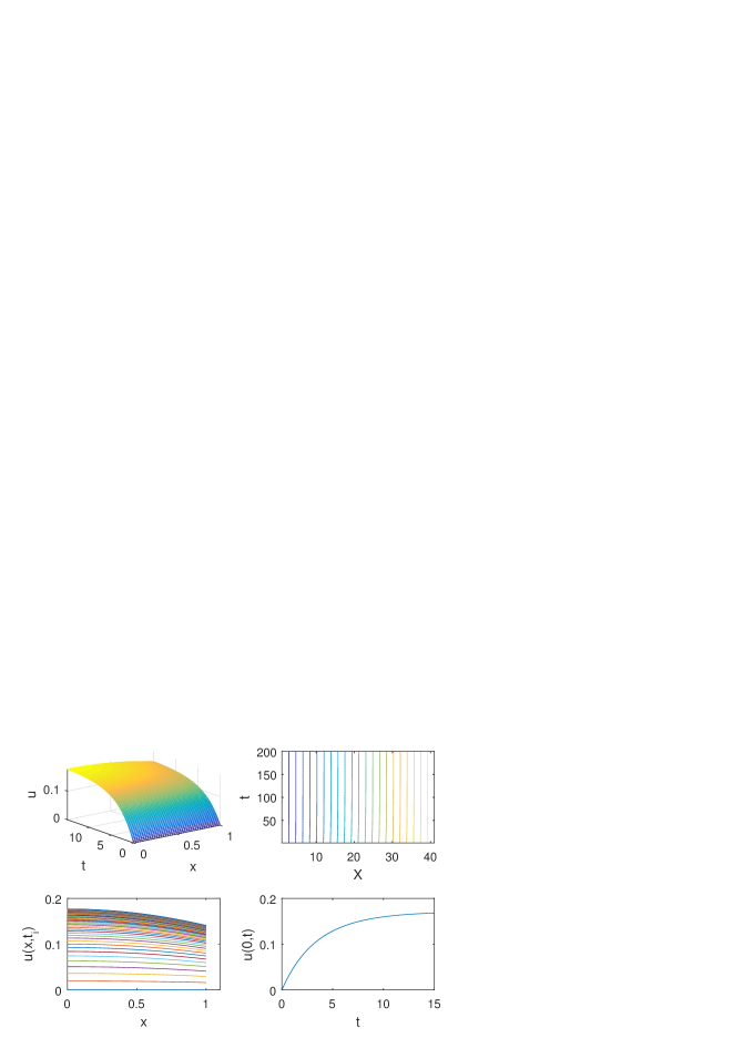
Figure 5. Form of the solution and various profiles of the local problem for $\lambda=0.05$, $\beta=1$

.

Figure 6 depicts the situation where the solution quenches in finite time. Again in the first of these graphs (top left) we plot the solution against space and time. In the second one (top right) we plot the moving mesh $X(i,t)$ against time. Here the motion of $X_{i}$’s captures the observed singularity, i.e. the finite-time quenching. In the third (bottom left) a sequence of profiles of the solution ($u(x,t_{i})$) for various time steps $t_{i}$ is presented. We can observe the increasing with time profiles of the solution. Finally in the fourth graph we plot the maximum of the solution $u(0,t)$ against time from which the quenching behaviour is revealed. The same parameters as in Figure 5 are used but with $\lambda=1$.

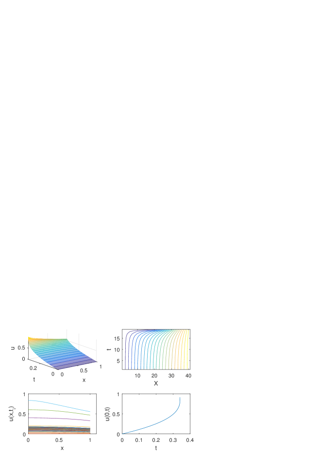
Figure 6. Form of the solution and various profiles of the local problem in the case of quenching for $\lambda=1$, and $\beta=1$

.

In the next Figure, 7 we plot the profiles of the solution maximum, $u(0,t)$ against time, for various $\lambda$’s and specifically for $\lambda=.7,\,.8,\,.9,\,1$. We observe that by increasing the value of the parameter $\lambda$ the quenching time decreases as it is expected.

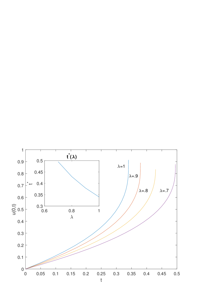
Figure 7. Form of the solution maximum against time for various values of the parameter $\lambda$ for the local problem for $\beta=1$

.

The Non-Local Problem

A similar set of simulations is presented for the case that $\alpha=1$ while the rest of the parameters, unless otherwise stated, are kept the same as in the experiment of Figure 5. In Figure 8 and for $\lambda=0.5$ the convergence of the solution towards a steady state is depicted.

Figure 8. Form of the solution and various profiles of the nonlocal problem, for ${\lambda}=0.5$, $\alpha=1$, $\beta=1$

.

In a similar set of graphs, see Figure 9 and for $\lambda=3$, we present the quenching behaviour of the solution.

Figure 9. Form of the solution and various profiles of the nonlocal problem for ${\lambda}=3$, $\alpha=1$, $\beta=1$

.

Moreover in Figure 10 we can observe the evolution of the quenching time as the value of the parameter $\lambda$ varies, something cannot be seen via our theoretical results. In particular,by increasing the parameter $\lambda$ results in a decreasing of quenching time. Here $\lambda=2.5,\,3,\,3.5,\,4.$

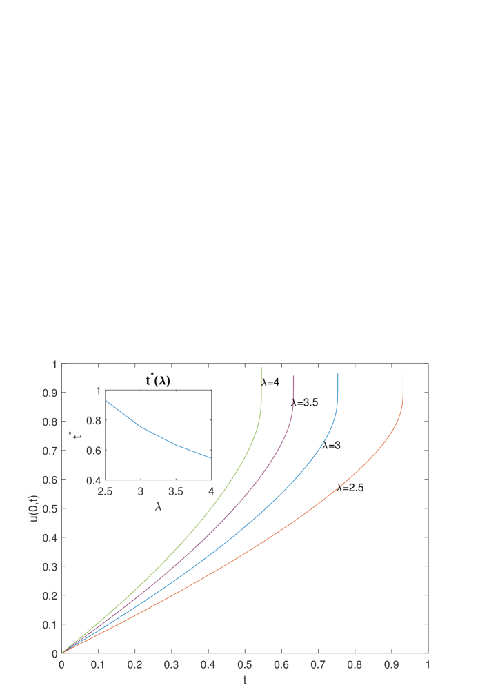
Figure 10. Form of the solution maximum against time for various values of the parameter $\lambda$ and with $\alpha=1$, $\beta=1$

.

Next in Figure 11(a) we plot a series of profiles for the maximum of the solution as the parameter $\alpha$ varies. Again such a behaviour cannot be unveiled via our analystical results in subsections 3.2 and 3.3. It is easily seen that by decreasing $\alpha$ the quenching time decreases too. The parameter $\alpha$ decreases from $1$ to the value $0$ whilst the parameter $\lambda$ is kept constant and equal to $\lambda=2$.

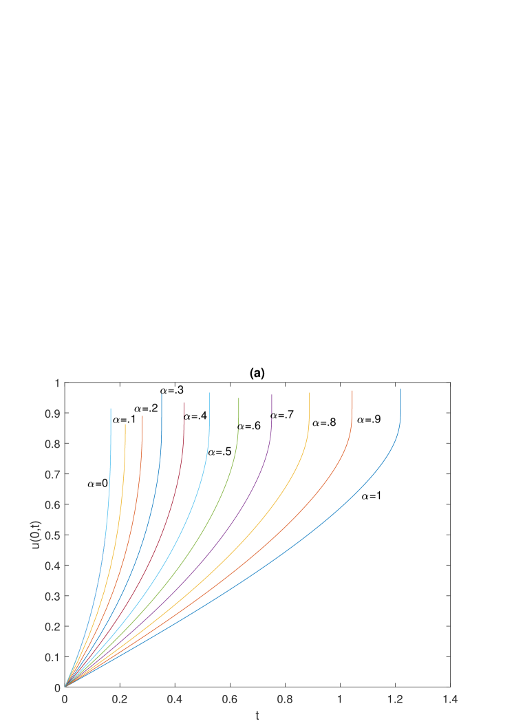
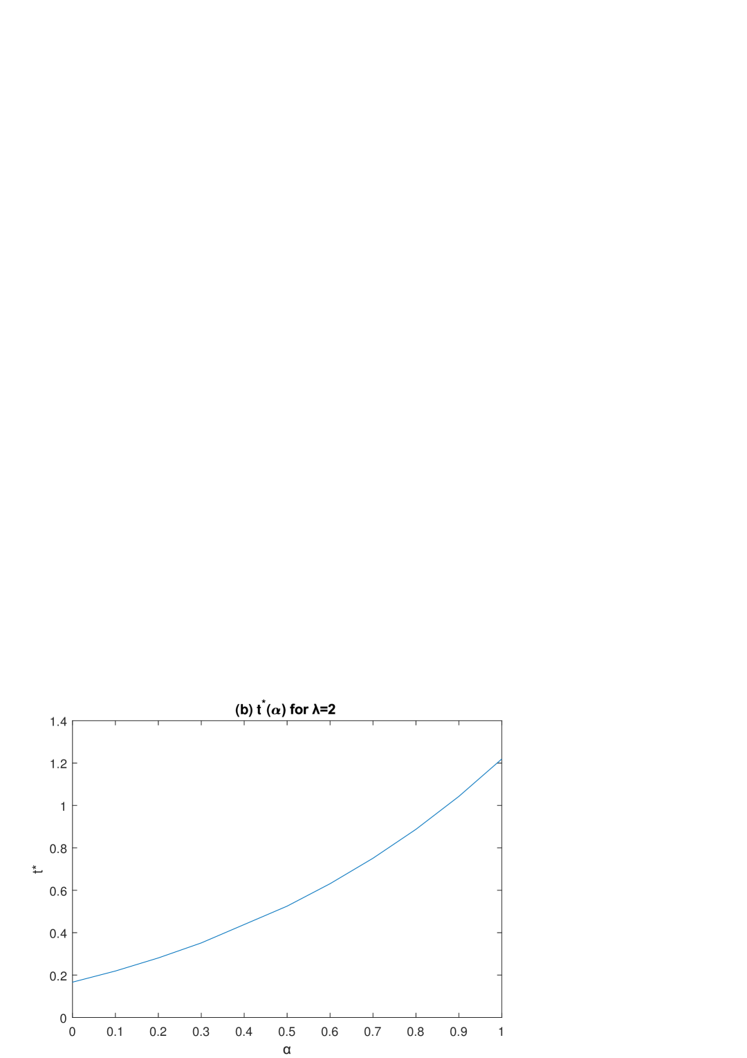
Figure 11. (a) Form of the solution maximum against time for various values of the parameter $\alpha$ for $\lambda=2$ and $\beta=1$. (b) Variation of the quenching time of the nonlocal problem with respect to the parameter $\alpha$.

The effect of the boundary parameter $\beta$ is unveiled by Figure 12(a), a fact cannot be easily seen by our theoretical results in section 3. Indeed, it is seen that by increasing $\beta$ a long-time behaviour resembles the one of the Dirichlet problem is derived. The variation of the quenching time $t^{*}$ of the nonlocal problem is depicted in a series of plots in Figures 11(b) and 12(b). In the first of them, Figure 11(b), we present a plot of $t^{*}(\alpha)$ while in the second 12(b), a plot of $t^{*}(\beta)$. In both cases was taken $\lambda=2$.

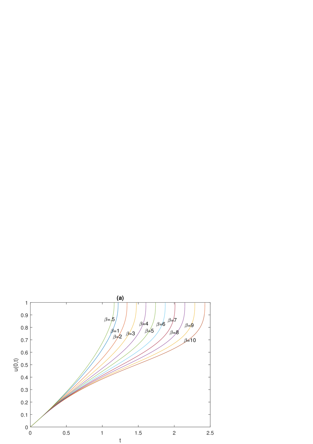
Figure 12. (a) Form of the solution maximum against time for various values of the parameter $\beta$ for $\lambda=2$ and $\alpha=1$. (b) Variation of the quenching time of the nonlocal problem with respect to the parameter $\beta$.

4.2. The Radial Symmetric Case

It has been already pointed out that the $2-$dimensional problem in the radially symmetric case is very interesting from the point of view of applications and thus we choose to provide a numerical treatment for it in the current subsection. For this purpose the aforementioned adaptive numerical scheme and specifically equation (4.1) can be modified accordingly with $u_{xx}+(N-1)r^{-1}u_{x}$ used in place of $u_{xx}$.

Initially we solve the local problem, i.e. problem (3.18) for $\alpha=0$ and the results are presented in Figure 13. Here we take $\beta=1$, $\lambda=0.05$ and we observe that the solution converges towards a steady state.

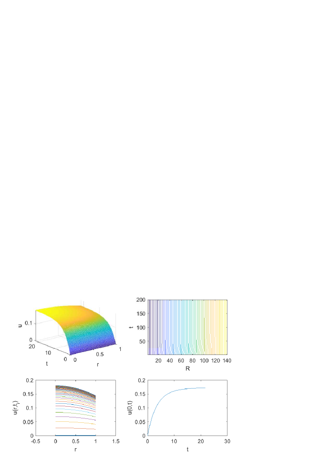
Figure 13. Form of the solution and various profiles of the local problem for the radial symmetric case for $\lambda=0.05$ and $\alpha=0$, $\beta=1$.

In Figure 14 we present an analogous simulation for the nonlocal problem. In that case we take $\alpha=1,\beta=1$, and $\lambda=0.2$ and we derive that the solution quenches in finite time.

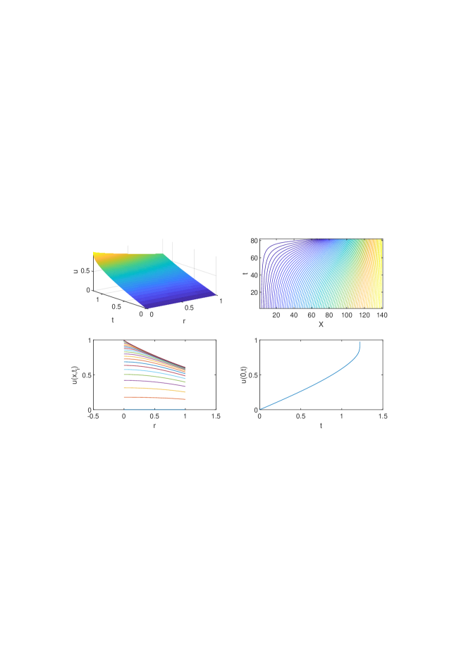
Figure 14. Form of the solution and various profiles of the nonlocal problem for the radial symmetric case for $\lambda=0.2$ and $\alpha=1$, $\beta=1$.

5. Discussion

In the current work we investigate a nonlocal parabolic problem with Robin boundary conditions associated with the operation of some idealized MEMS device. In the first part we deliver a thorough investigation of the associated steady-state problem and we derive some estimates of the pull-in voltage, which is the controlling parameter of the model. In particular, and for the $N-$dimensional case , $N>1,$ in order to derive sharp estimates for the pull-in voltage we had to show, as a very interesting by-product, a Pohožaev’s type identity for Robin boundary conditions. To the best of our knowledge such a result has not been available in the literature.

In the second part of this work, existence and uniqueness results together with long time behaviour of time-dependent problem are discussed. In particular, we focus on the investigation of the phenomenon of quenching (i.e. the so called touching down in the context of MEMS literature). We first examine the quenching behaviour on a general domain, whilst later in order to derive an optimal quenching result we restrict ourselves to the radially symmetric case.

Finally we close our investigation by the implementation of an adaptive numerical method, [5], for the solution of the time-dependent problem. We actually perform a series of numerical experiments verifying the obtained analytical results as well as revealing qualitative features of nonlocal problem (1.1) do not arise from our analytical approach. Additionally, some further numerical experiments are performed to determine the quenching profile of the solution in the radially symmetric case.

References

- [1] R.C. Ackerberg, On a nonlinear differential equation of electrohydrodynamics, Proc. Roy. Soc. A 312 (1969) 129–140.
- [2] M. Al-Refai, N.I. Kavallaris, M. A. Hajji, Monotone iterative sequences for nonlocal elliptic problems, Euro. Jnl. Appl. Mathematics 22(6), 533–552.
- [3] H. Amann, Fixed point equations and nonlinear eigenvalue problems in ordered Banach spaces, SIAM Rev. 18 (1976), 620–-709.
- [4] C. Bandle, Isoperimetric inequalities and applications, Monographs and Studies in Mathematics, 7., Pitman, Boston-London, 1980.
- [5] C. J. Budd, J. F. Williams, How to adaptively resolve evolutionary singularities in differential equations with symmetry, J. Eng. Math. 66 (2010) 217–236.
- [6] E.K. Chan & R.W. Dutton, Effects of Capacitors, Resistors and Residual Change on the Static and Dynamic Performance of Electrostatically Actuated Devices, Proceedings of SPIE, 3680, (1999), 120–130.
- [7] O. Drosinou, N.I. Kavallaris and C.V. Nikolopoulos, Impacts of noise on quenching of some models arising in MEMS technology, arXiv:2012.10922v1.
- [8] G. K. Duong & H. Zaag, Profile of a touch-down solution to a nonlocal MEMS model, Math. Models Methods Appl. Sci. 29 (7) (2019) 1279–1348.
- [9] P. Esposito, N. Ghoussoub, Y. Guo, Mathematical analysis of partial differential equations modeling electrostatic MEMS, Courant Lecture Notes in Mathematics, 20. Courant Institute of Mathematical Sciences, New York, American Mathematical Society, Providence, RI, 2010.
- [10] L. C. Evans, Partial Differential Equations, Second Edition, American Mathematical Society, 2010.
- [11] S. Filippas & J-S. Guo, Quenching profiles for one-dimensional semilinear heat equations, Quart. Appl. Math. 51 (1993) 713–729.
- [12] A. Friedman, B. McLeod, Blow-up of positive solutions of semilinear heat equations, Indiana Univ. Math. J. 34 (1985) 425–447.
- [13] Gidas, B., Ni, Wei Ming & Nirenberg, L., Symmetry and related properties via the maximum principle, Comm. Math. Phys. 68 (1979), no. 3, 209–243.
- [14] Y. Guo, Dynamical solutions of singular wave equations modeling electrostatic MEMS, SIAM J. Appl. Dyn. Syst., 9 (2010), 1135–1163.
- [15] J-S. Guo, On a quenching problem with the Robin boundary condition, Nonlinear Analysis: Theory, Methods & Applications, 179, (1991), 803–809.
- [16] J.-S. Guo, Recent developments on a nonlocal problem arising in the micro-electromechanical system, Tamkang Jour. Mathematics 45(3), (2014), 229–241.
- [17] J.-S. Guo & B. Hu Quenching rate for a nonlocal problem arising in the micro-electro mechanical system, J. Differential Equations 264 (2018), no. 5, 3285–3311.
- [18] J.-S. Guo, B. Hu & C.-J. Wang, A nonlocal quenching problem arising in micro-electro mechanical systems, Quart. Appl. Math. 67 (2009) 725–734.
- [19] J.-S. Guo & N.I. Kavallaris, On a nonlocal parabolic problem arising in electromechanical MEMS control. Disc. Cont. Dynam. Systems 32 (2012) 1723–1746.
- [20] J.-S. Guo, N.I. Kavallaris, C.-Y. Yu & C.-Y. Yu Bifurcation diagram of a Robin boundary value problem arising in MEMS, arXiv:2007.03977v1.
- [21] Y. Guo, On the partial differential equations of electrostatic MEMS devices III: refined touchdown behavior, J. Diff. Eqns. 244 (2008) 2277–2309.
- [22] Y. Guo, Z. Pan, M.J. Ward, Touchdown and pull-in voltage behavior of a MEMS device with varying dielectric properties, SIAM J.Appl. Math. 166 (2006) 309–338.
- [23] K-M. Hui, The existence and dynamic properties of a parabolic nonlocal MEMS equation, Nonlinear Analysis: Theory, Methods & Applications 74 (2011) 298–316.
- [24] N.I. Kavallaris, Blow-up and global existence of solutions of some nonlocal problems arising in Ohmic heating process, Ph.D Thesis, National Technical University of Athens (2000) (in Greek).
- [25] N. I. Kavallaris, Asymptotic behaviour and blow-up for a nonlinear diffusion problem with a nonlocal source term, Proc. Edinb. Math. Soc. 47, (2004) 375–-395.
- [26] N.I. Kavallaris & T. Nadzieja, On the blow-up of the nonlocal thermistor problem, Proc. Edin. Math. Soc. 50, (2007), 389–409.
- [27] N.I. Kavallaris, T. Miyasita, T. Suzuki, Touchdown and related problems in electrostatic MEMS device equation, Nonlinear Diff. Eqns. Appl. 15 (2008), 363–385.
- [28] N. I. Kavallaris, A. A. Lacey, C. V. Nikolopoulos, D. E. Tzanetis, A hyperbolic nonlocal problem modelling MEMS technology, Rocky Mountain J. Math. 41 (2011), 505–534.
- [29] N. I. Kavallaris, A. A. Lacey, C. V. Nikolopoulos, D. E. Tzanetis, On the quenching behaviour of a semilinear wave equation modelling MEMS technology, Discrete and Continuous Dynamical Systems - Series A, 35(3), (2015), 1009-1037.
- [30] N. I. Kavallaris, A. A. Lacey, C. V. Nikolopoulos, On the quenching of a nonlocal parabolic problem arising in electrostatic MEMS control, Nonlinear Analysis, 138, (2016), 189–206.
- [31] N. I. Kavallaris, Quenching solutions of a stochastic parabolic problem arising in electrostatic MEMS control, Math. Methods Appl. Sci. 41 (2018), no. 3, 1074–1082.
- [32] N.I. Kavallaris & T. Suzuki, Non-Local Partial Differential Equations for Engineering and Biology: Mathematical Modeling and Analysis, Mathematics for Industry, Vol. 31 Springer Nature 2018.
- [33] O. Ladyženskaja, V.A. Solonnikov & N.N. Ural’ceva, Linear and Quasi-Linear Equations of Parabolic Type, Amer. Math. Soc. Providence, R.I. 1968.
- [34] A.A. Lacey, Thermal runaway in a nonlocal problem modelling Ohmic heating: Part II : General proof of blow-up and asymptotics of runaway, Euro Jl. Appl. Maths. 6, (1995), 201–224 .
- [35] H.A. Levine, Quenching, nonquenching, and beyond quenching for solution of some parabolic equations, Ann. Mat. Pura Appl. 155 (1989), 243–260.
- [36] F. Merle & H. Zaag, Reconnection of vortex with the boundary and finite time quenching, Nonlinearity 10 (1997) 1497–1550.
- [37] C.V. Pao, Nonlinear Parabolic and Elliptic Equations, Springer 1992.
- [38] J.A. Pelesko, D.H. Bernstein, Modeling MEMS and NEMS, Chapman Hall and CRC Press, 2002.
- [39] J.A. Pelesko and X.Y.Chen, Electrostatic deflections of circular elastic membranes, J. Electrostatics 57 (2003), 1–12.
- [40] J.A. Pelesko and A.A. Triolo, Non-local problems in MEMS device control, J. Engrg. Math., 41 (2001), 345–366.
- [41] J.A. Pelesko, Mathematical Modeling of Electrostatic MEMS with Taylored Dielectric Properties SIAM Journal of Applied Mathematics, 62, 3 (2002) pp. 888–908.
- [42] S. I. Pohožaev, On the eigenfunctions of the equation , Dokl. Akad. Nauk SSSR, 165 (1965), 36–39.
- [43] Quittner, P. & Souplet, P. Superlinear parabolic problems. Blow-up, global existence & steady states. Birkhäuser Adv. Texts Basler Lehrbücher. Birkhäuser 2007.
- [44] J.J. Seeger & S.B. Crary, Stabilization of electrostatically actuated mechanical devices, Proceedings of the 1997 International Conference on Solid-State Sensors and Actuators, (1997), 1133–1336 .
- [45] J.J. Seeger & S.B. Crary, Analysis and simulation of MOS capacitor feedback for stabilizing electrostatically actuated ,echanical devices, Second International Conference on the Simulation and Design of Microsystems and Microstructures-MICROSIM97, (1997), 199–208.
- [46] G.I. Taylor, The coalescence of closely spaced drops when they are at different electric potentials, Proc. Roy. Soc. A, 306 (1968) 423–434.
- [47] M. Younis, MEMS Linear and Nonlinear Statics and Dynamics, Springer, New York, 2011.