Efficient Neural Interaction Function Search
for Collaborative Filtering

Abstract.

In collaborative filtering (CF), interaction function (IFC) play the important role of capturing interactions among items and users. The most popular IFC is the inner product, which has been successfully used in low-rank matrix factorization. However, interactions in real-world applications can be highly complex. Thus, other operations (such as plus and concatenation), which may potentially offer better performance, have been proposed. Nevertheless, it is still hard for existing IFCs to have consistently good performance across different application scenarios. Motivated by the recent success of automated machine learning (AutoML), we propose in this paper the search for simple neural interaction functions (SIF) in CF. By examining and generalizing existing CF approaches, an expressive SIF search space is designed and represented as a structured multi-layer perceptron. We propose an one-shot search algorithm that simultaneously updates both the architecture and learning parameters. Experimental results demonstrate that the proposed method can be much more efficient than popular AutoML approaches, can obtain much better prediction performance than state-of-the-art CF approaches, and can discover distinct IFCs for different data sets and tasks.

Table 1. Popular human-designed interaction functions (IFC) for CF, where $\bm{H}$ is a parameter to be trained. SIF searches a proper IFC from the validation set (i.e., by AutoML), while others are all designed by experts.

	IFC	operation	space	predict time	recent examples
	$\left\langle\bm{u}_{i},\bm{v}_{j}\right\rangle$	inner product	$O((m+n)k)$	$O(k)$	MF (Koren, 2008), FM (Rendle, 2012)
	$\bm{u}_{i}-\bm{v}_{j}$	plus (minus)	$O((m+n)k)$	$O(k)$	CML (Hsieh et al., 2017)
	$\max\left(\bm{u}_{i},\bm{v}_{j}\right)$	max, min	$O((m+n)k)$	$O(k)$	ConvMF (Kim et al., 2016)
human-designed	$\sigma\left([\bm{u}_{i};\bm{v}_{j}]\right)$	concat	$O((m+n)k)$	$O(k)$	Deep&Wide (Cheng et al., 2016)
	$\sigma\left(\bm{u}_{i}\odot\bm{v}_{j}+\bm{H}\left[\bm{u}_{i};\bm{v}_{j}\right]\right)$	multi, concat	$O((m+n)k)$	$O(k^{2})$	NCF (He et al., 2017)
	$\bm{u}_{i}*\bm{v}_{j}$	conv	$O((m+n)k)$	$O(k\log(k))$	ConvMF (Kim et al., 2016)
	$\bm{u}_{i}\otimes\bm{v}_{j}$	outer product	$O((m+n)k)$	$O(k^{2})$	ConvNCF (He et al., 2018)
AutoML	SIF (proposed)	searched	$O((m+n)k)$	$O(k)$	——

1. Introduction

Collaborative filtering (CF) (Herlocker et al., 1999; Su and Khoshgoftaar, 2009) is an important topic in machine learning and data mining. By capturing interactions among the rows and columns in a data matrix, CF predicts the missing entries based on the observed elements. The most famous CF application is the recommender system (Koren, 2008). The ratings in such systems can be arranged as a data matrix, in whch the rows correspond to users, the columns are items, and the entries are collected ratings. Since users usually only interact with a few items, there are lots of missing entries in the rating matrix. The task is to estimate users’ ratings on items that they have not yet explored. Due to the good empirical performance, CF also have been used in various other applications. Examples include image inpainting in computer vision (Ji et al., 2010), link prediction in social networks (Kim and Leskovec, 2011) and topic modeling for text analysis (Wang and Blei, 2011). More recently, CF is also extended to tensor data (i.e., higher-order matrices) (Kolda and Bader, 2009) for the incorporation of side information (such as extra features (Karatzoglou et al., 2010) and time (Lei et al., 2009)).

In the last decade, low-rank matrix factorization (Koren, 2008; Mnih and Salakhutdinov, 2008) has been the most popular approach to CF. It can be formulated as the following optimization problem:

(1) $$\min_{\bm{U},\bm{V}}\sum\nolimits_{(i,j)\in\Omega}\ell\left(\bm{u}_{i}^{\top}\bm{v}_{j},\bm{O}_{ij}\right)+\frac{\lambda}{2}\|\bm{U}\|_{F}^{2}+\frac{\lambda}{2}\|\bm{V}\|_{F}^{2},$$

where $\ell$ is a loss function. The observed elements are indicated by $\Omega$ with values given by the corresponding positions in matrix $\bm{O}\in\mathbb{R}^{m\times n}$, $\lambda\geq 0$ is a hyper-parameter, and $\bm{u}_{i},\bm{v}_{j}\in\mathbb{R}^{k}$ are embedding vectors for user $i$ and item $j$, respectively. Note that (1) captures interactions between user $\bm{u}_{i}$ and item $\bm{v}_{j}$ by the inner product. This achieves good empirical performance, enjoys sound statistical guarantees (Candès and Recht, 2009; Recht et al., 2010) (e.g., the data matrix can be exactly recovered when $\bm{O}$ satisfies certain incoherence conditions and the missing entires follow some distributions), and fast training (Mnih and Salakhutdinov, 2008; Gemulla et al., 2011) (e.g., can be trained end-to-end by stochastic optimization).

While the inner product has many benefits, it may not yield the best performance for various CF tasks due to the complex nature of user-item interactions. For example, if $i$th and $j$th users like the $k$th item very much, their embeddings should be close to each other (i.e., $\|\bm{u}_{i}-\bm{u}_{j}\|_{2}$ is small). This motivates the usage of the plus operation (He et al., 2017; Hsieh et al., 2017), as the triangle inequality ensures $\|\bm{u}_{i}-\bm{u}_{j}\|_{2}\leq\|\bm{u}_{i}-\bm{v}_{k}\|_{2}+\|\bm{u}_{j}-\bm{v}_{k}\|_{2}$. Other operations (such as concatenation and convolution) have also outperformed the inner product on many CF tasks (Rendle, 2012; Kim et al., 2016; He et al., 2018). Due to the success of deep networks (Goodfellow et al., 2016), the multi-layer perceptron (MLP) is recently used as the interaction function (IFC) in CF (Cheng et al., 2016; He et al., 2017; Xue et al., 2017), and achieves good performance. However, choosing and designing an IFC is not easy, as it should depend on the data set and task. Using one simple operation may not be expressive enough to ensure good performance. On the other hand, directly using a MLP leads to the difficult and time-consuming task of architecture selection (Zoph and Le, 2017; Baker et al., 2017; Zhang et al., 2019). Thus, it is hard to have a good IFC across different tasks and data sets (Dacrema et al., 2019).

In this paper, motivated by the success of automated machine learning (AutoML) (Hutter et al., 2018; Yao and Wang, 2018), we consider formulating the search for interaction functions (SIF) as an AutoML problem. Inspired by observations on existing IFCs, we first generalize the CF objective and define the SIF problem. These observations also help to identify a domain-specific and expressive search space, which not only includes many human-designed IFCs, but also covers new ones not yet explored in the literature. We further represent the SIF problem, armed with the designed search space, as a structured MLP. This enables us to derive an efficient search algorithm based on one-shot neural architecture search (Liu et al., 2018; Xie et al., 2018; Yao et al., 2020). The algorithm can jointly train the embedding vectors and search IFCs in a stochastic end-to-end manner. We further extend the proposed SIF, including both the search space and one-shot search algorithm, to handle tensor data. Finally, we perform experiments on CF tasks with both matrix data (i.e., MovieLens data) and tensor data (i.e., Youtube data). The contributions of this paper are highlighted as follows:

• The design of interaction functions is a key issue in CF, and is also a very hard problem due to varieties in the data sets and tasks (Table 1). We generalize the objective of CF, and formulate the design of IFCs as an AutoML problem. This is also the first work which introduces AutoML techniques to CF.

• By analyzing the formulations of existing IFCs, we design an expressive but compact search space for the AutoML problem. This covers previous IFCs given by experts as special cases, and also allows generating novel IFCs that are new to the literature. Besides, such a search space can be easily extended to handle CF problems on tensor data.

• We propose an one-shot search algorithm to efficiently optimize the AutoML problem. This algorithm can jointly update the architecture of IFCs (searched on the validation set) and the embedding vectors (optimized on the training set).

• Empirical results demonstrate that, the proposed algorithm can find better IFCs than existing AutoML approaches, and is also much more efficient. Compared with the human-designed CF methods, the proposed algorithm can achieve much better performance, while the computation cost is slightly higher than that from fine-tuning by experts. To shed light on the design of IFCs, we also perform a case study to show why better IFCs can be found by the proposed method.

Notations. Vectors are denoted by lowercase boldface, and matrices by uppercase boldface. For two vectors $\bm{x}$ and $\bm{y}$, $\left\langle\bm{x},\bm{y}\right\rangle$ is the inner product, $\bm{x}\odot\bm{y}$ is the element-wise product, $\bm{x}\otimes\bm{y}$ is the outer product, $[\bm{x};\bm{y}]$ concatenates (denoted “concat”) two vectors to a longer one, and $\bm{x}*\bm{y}$ is the convolution (denoted “conv”). $\text{Tr}(\bm{X})$ is the trace of a square matrix $\bm{X}$, and $\|\bm{X}\|_{F}$ is the Frobenius norm. $\|\bm{x}\|_{2}$ is the $\ell_{2}$-norm of a vector $\bm{x}$, and $\|\bm{x}\|_{0}$ counts its number of nonzero elements. The proximal step (Parikh and Boyd, 2013) associated with a function $g$ is defined as $\text{prox}_{g}(\bm{z})=\arg\min_{\bm{x}}\frac{1}{2}\|\bm{z}-\bm{x}\|_{2}^{2}+g(\bm{x})$. Let $\mathcal{S}$ be a constraint and $\mathbb{I}(\cdot)$ be the indicator function, i.e., if $\bm{x}\in\mathcal{S}$ then $\mathbb{I}(\mathcal{S})=0$ and $\infty$ otherwise, then $\text{prox}_{\mathbb{I}(\mathcal{S})}(\bm{z})=\arg\min_{\bm{x}}\frac{1}{2}\|\bm{z}-\bm{x}\|_{2}^{2}$ s.t. $\bm{x}\in\mathcal{S}$ is also the projection operator, which maps $\bm{z}$ on $\mathcal{S}$.

2. Related Works

2.1. Interaction Functions (IFCs)

As discussed in Section 1, the IFC is key to CF. Recently, many CF models with different ICFs have been proposed. Examples include the factorization machine (FM) (Rendle, 2012), collaborative metric learning (CML) (Hsieh et al., 2017), convolutional matrix factorization (ConvMF) (Kim et al., 2016), Deep & Wide (Cheng et al., 2016), neural collaborative filtering (NCF) (He et al., 2017), and convolutional neural collaborative filtering (ConvNCF) (He et al., 2018). As can be seen from Table 1, many operations other than the simple inner product have been used. Moreover, they have the same space complexity (linear in $m$, $n$ and $k$), but different time complexities.

The design of IFCs depends highly on the given data and task. As shown in a recent benchmark paper (Dacrema et al., 2019), no single IFC consistently outperforms the others across all CF tasks (Su and Khoshgoftaar, 2009; Aggarwal, 2017). Thus, it is important to either select a proper IFC from a set of customized IFC’s designed by humans, or to design a new IFC which has not been visited in the literature.

2.2. Automated Machine Learning (AutoML)

To ease the use and design of better machine learning models, automated machine learning (AutoML) (Hutter et al., 2018; Yao and Wang, 2018) has become a recent hot topic. AutoML can be seen as a bi-level optimization problem, as we need to search for hyper-parameters and design of the underlying machine learning model.

2.2.1. General Principles

In general, the success of AutoML hinges on two important questions:

• What to search: In AutoML, the choice of the search space is extremely important. On the one hand, the space needs to be general enough, meaning that it should include human wisdom as special cases. On the other hand, the space cannot be too general, otherwise the cost of searching in such a space can be too expensive (Zoph et al., 2017; Liu et al., 2018). For example, early works on neural architecture search (NAS) use reinforcement learning (RL) to search among all possible designs of a convolution neural network (CNN) (Baker et al., 2017; Zoph and Le, 2017). This takes more than one thousand GPU days to obtain an architecture with performance comparable to the human-designed ones. Later, the search space is partitioned into blocks (Zoph et al., 2017), which helps reduce the cost of RL to several weeks.

• How to search efficiently: Once the search space is determined, the search algorithm then matters. Unlike convex optimization, there is no universal and efficient optimization for AutoML (Hutter et al., 2018). We need to invent efficient algorithms to find good designs in the space. Recently, gradient descent based algorithms are adapted for NAS (Yao et al., 2020; Liu et al., 2018; Xie et al., 2018), allowing joint update of the architecture weights and learning parameters. This further reduces the search cost to one GPU day.

2.2.2. One-Shot Architecture Search Algorithms

Recently, one-shot architecture search (Bender et al., 2018) methods such as DARTS (Liu et al., 2018) and SNAS (Xie et al., 2018), have become the most popular NAS methods for the efficient search of good architectures. These methods construct a supernet, which contains all possible architectures spanned by the selected operations, and then jointly optimize the network weights and architectures’ parameters by stochastic gradient descent. The state-of-the-art is NASP (Yao et al., 2020) (Algorithm 1). Let $\bm{\alpha}=[a_{k}]\in\mathbb{R}^{d}$, with $a_{k}$ encoding the weight of the $k$th operation, and $\bm{X}$ be the parameter. In NSAP, the selected operation $\bar{\mathcal{O}}(\bm{X})$ is represented as

(2) $$\bar{\mathcal{O}}(\bm{X})=\sum\nolimits_{k=1}^{d}a_{k}\mathcal{O}_{k}(\bm{X}),~{}\text{\;where\;}~{}\bm{\alpha}\in\mathcal{C}_{1}\cap\mathcal{C}_{2},$$

$\mathcal{O}_{k}(\cdot)$ is the $k$th operation in $\mathcal{O}$,

(3) $$\mathcal{C}_{1}=\left\{\bm{\alpha}\,|\,\|\bm{\alpha}\|_{0}=1\right\}\quad\text{and}\quad\mathcal{C}_{2}=\left\{\bm{\alpha}\,|\,0\leq\alpha_{k}\leq 1\right\}.$$

The discrete constraint in (2) forces only one operation to be selected. The search problem is then formulated as

(4) $$\min_{\bm{\alpha}}\bar{\mathcal{L}}\left(\bm{w}^{*}(\bm{\alpha}),\bm{\alpha}\right),\text{\;s.t.\;}\begin{cases}\bm{w}^{*}(\bm{\alpha})=\arg\min_{\bm{w}}\mathcal{L}\left(\bm{w},\bm{\alpha}\right)\\ \bm{\alpha}\in\mathcal{C}_{1}\cap\mathcal{C}_{2}\end{cases},$$

where $\bar{\mathcal{L}}$ (resp. $\mathcal{L}$) is the loss on validation (resp. training) data. As NASP targets at selecting and updating only one operation, it maintains two architecture representations: a continuous $\bm{\alpha}$ to be updated by gradient descent (step 4 in Algorithm 1) and a discrete $\bar{\bm{\alpha}}$ (steps 3 and 5). Finally, the network weight $\bm{w}$ is optimized on the training data in step 6. The following Proposition shows closed-form solutions to the proximal step in Algorithm 1.

Algorithm 1 Neural architecture search by proximal iterations (NASP) algorithm (Yao et al., 2020).

1:  require: A mixture of operations $\bar{\mathcal{O}}$ parametrized by (2), parameter $\bm{w}$ and stepsize $\eta$;

2:  while not converged do

3:     Obtain discrete architecture representation $\bar{\bm{\alpha}}=\text{prox}_{\mathcal{C}_{1}}(\bm{\alpha})$;

4:     Update continuous architecture representation

$$\bm{\alpha}=\text{prox}_{\mathcal{C}_{2}}(\bm{\alpha}-\nabla_{\bar{\bm{\alpha}}}\bar{\mathcal{L}}(\bar{\bm{w}},\bar{\bm{\alpha}})),$$

where $\bar{\bm{w}}\!=\!\bm{w}\!-\!\eta\nabla_{\bm{w}}\mathcal{L}(\bm{w},\bar{\bm{\alpha}})$ (is an approximation to $\bm{w}^{*}(\bar{\bm{\alpha}})$);

5:     Obtain new discrete architecture $\bar{\bm{\alpha}}=\text{prox}_{\mathcal{C}_{1}}(\bm{\alpha})$;

6:     Update $\bm{w}$ using $\nabla_{\bm{w}}\mathcal{L}(\bm{w},\bar{\bm{\alpha}})$ with $\bar{\bm{\alpha}}$;

7:  end while

8:  return  Searched architecture $\bar{\bm{\alpha}}$.

Proposition 2.1 ((Parikh and Boyd, 2013; Yao et al., 2020)).

Let $\bm{z}\in\mathbb{R}^{d}$. (i) $\text{prox}_{\mathcal{C}_{1}}(\bm{z})=z_{i}\bm{e}_{i}$, where $i=\arg\max_{i=1,\cdots,d}|z_{i}|$, and $\bm{e}_{i}$ is a one-hot vector with only the $i$th element being 1. (ii) $\text{prox}_{\mathcal{C}_{2}}(\bm{z})=\tilde{\bm{z}}$, where $\tilde{\bm{z}}_{i}=z_{i}$ if $z_{i}\in[0,1]$, $\tilde{\bm{z}}_{i}=0$ if $z_{i}<0$, and $\tilde{\bm{z}}_{i}=1$ otherwise.

3. Proposed Method

In Section 2, we have discussed the importance of IFCs, and the difficulty of choosing or designing one for the given task and data. Similar observations have also been made in designing neural networks, which motivates NAS methods for deep networks (Baker et al., 2017; Zoph and Le, 2017; Zoph et al., 2017; Xie et al., 2018; Liu et al., 2018; Bender et al., 2018; Yao et al., 2020). Moreover, NAS has been developed as a replacement of humans, which can discover data- and task-dependent architectures with better performance. Besides, there is no absolute winner for IFCs (Dacrema et al., 2019), just like the deep network architecture also depends on data sets and tasks. These inspire us to search for proper IFCs in CF by AutoML approaches.

3.1. Problem Definition

First, we define the AutoML problem here and identify an expressive search space for IFCs, which includes the various operations in Table 1. Inspired by generalized matrix factorization (He et al., 2017; Xue et al., 2017) and objective (1), we propose the following generalized CF objective:

(5) $$\min F(\bm{U},\bm{V},\bm{w})\equiv \sum\nolimits_{(i,j)\in\Omega}\ell(\bm{w}^{\top}f\left(\bm{u}_{i},\bm{v}_{j}\right),\bm{O}_{ij})$$

$$+\frac{\lambda}{2}\|\bm{U}\|_{F}^{2}+\frac{\lambda}{2}\|\bm{V}\|_{F}^{2},\;\text{s.t.}\;\|\bm{w}\|_{2}\leq 1,$$

where $f$ is the IFC (which takes the user embedding vector $\bm{u}_{i}$ and item embedding vector $\bm{v}_{j}$ as input, and outputs a vector), and $\bm{w}$ is a learning parameter. Obviously, all the IFCs in Table 1 can be represented by using different $f$’s. The following Proposition shows that the constraint $\|\bm{w}\|_{2}\leq 1$ is necessary to ensure existence of a solution.

Proposition 3.1.

If $f$ is an operation shown in Table 1 and the $\ell_{2}$-constraint on $\bm{w}$ is removed, then $F$ in (5) has no nonzero optimal solution when $\lambda>0$ (proof is in Appendix A.3).

Based on above objective, we now define the AutoML problem, i.e., searching interaction functions (SIF) for CF, here.

Definition 3.0 (AutoML problem).

Let $\mathcal{M}$ be a performance measure (the lower the better) defined on the validation set $\bar{\Omega}$ (disjoint from $\Omega$), and $\mathcal{F}$ be a family of vector-valued functions with two vector inputs. The problem of searching for an interaction function (SIF) is formulated as

(6) $$f^{*} =\arg\min_{f\in\mathcal{F}}\sum\nolimits_{(i,j)\in\bar{\Omega}}\mathcal{M}(f(\bm{u}^{*}_{i},\bm{v}^{*}_{j})^{\top}\bm{w}^{*},\bm{O}_{ij})$$

$$\;\text{s.t.}\;\left[\bm{U}^{*},\bm{V}^{*},\bm{w}^{*}\right]=\underset{\bm{U},\bm{V},\bm{w}}{\arg\min}F(\bm{U},\bm{V},\bm{w}),$$

where $\bm{u}^{*}_{i}$ (resp. $\bm{v}^{*}_{j}$) is the $i$th column of $\bm{U}^{*}$ (resp. $j$th column of $\bm{V}^{*}$).

Similar to other AutoML problems (such as auto-sklearn (Feurer et al., 2015), NAS (Baker et al., 2017; Zoph and Le, 2017) and AutoML in knowledge graph (Zhang et al., 2019)), SIF is a bi-level optimization problem (Colson et al., 2007). On the top level, a good architecture $f$ is searched based on the validation set. On the lower level, we find the model parameters using $F$ on the training set. Due to the nature of bi-level optimization, AutoML problems are difficult to solve in general. In the following, we show how to design an expressive search space (Section 3.2), propose an efficient one-shot search algorithm (Section 3.3), and extend the proposed method to tensor data (Section 3.4).

3.2. Designing a Search Space

Because of the powerful approximation capability of deep networks (Raghu et al., 2017), NCF (He et al., 2017) and Deep&Wide (Cheng et al., 2016) use a MLP as $f$. SIF then becomes searching a suitable MLP from the family $\mathcal{F}$ based on the validation set (details are in Appendix A.1), where both the MLP architecture and weights are searched. However, a direct search of this MLP can be expensive and difficult, since determining its architecture is already an extremely time-consuming problem as observed in the NAS literature (Zoph et al., 2017; Liu et al., 2018). Thus, as in Section 2.2, it is preferable to use a simple but expressive search space that exploits domain-specific knowledge from experts.

Notice that Table 1 contains operations that are

• Micro (element-wise): a possibly nonlinear function operating on individual elements, and

• Marco (vector-wise): operators that operate on the whole input vector (e.g., minus and multiplication).

Inspired by previous attempts that divide the NAS search space into micro and macro levels (Zoph et al., 2017; Liu et al., 2018), we propose to first search for a nonlinear transform on each single element, and then combine these element-wise operations at the vector-level. Specifically, let $\mathcal{O}$ be an operator selected from multi, plus, min, max, concat, $g(\beta;\bm{x})\in{\mathbb{R}}$ be a simple nonlinear function with input $\beta\in{\mathbb{R}}$ and hyper-parameter $\bm{x}$. We construct a search space $\mathcal{F}$ for (6), in which each $f$ is

(7) $$f(\bm{u}_{i},\bm{v}_{j})=\mathcal{O}(\dot{\bm{u}}_{i},\dot{\bm{v}}_{j}),$$

with $\left[\dot{\bm{u}}_{i}\right]_{l}=g\left(\left[\bm{u}_{i}\right]_{l};\bm{p}\right)$ and $[\dot{\bm{v}}_{j}]_{l}=g([\bm{v}_{j}]_{l};\bm{q})$ where $\left[\bm{u}_{i}\right]_{l}$ (resp. $[\bm{v}_{j}]_{l}$) is the $l$th element of $\bm{u}_{i}$ (resp. $[\bm{v}_{j}]_{l}$), and $\bm{p}$ (resp. $\bm{q}$) is the hyper-parameter of $g$ transforming the user (resp. item) embeddings. Note that we omit the convolution and outer product (vector-wise operations) from $\mathcal{O}$ in (7), as they need significantly more computational time and have inferior performance than the rest (see Section 4.4). Besides, we parameterize $g$ with a very small MLP with fixed architecture (single input, single output and five sigmoid hidden units) for the element-wise level in (7), and the $\ell_{2}$-norms of the weights, i.e., $\bm{p}$ and $\bm{q}$ in (7), are constrained to be smaller than or equal to 1.

This search space $\mathcal{F}$ meets the requirements for AutoML in Section 2.2. First, as it involves an extra nonlinear transformation, it contains operations that are more general than those designed by experts in Table 1. This expressiveness leads to better performance than the human-designed models in the experiments (Section 4.2). Second, the search space is much more constrained than that of a general MLP mentioned above, as we only need to select an operation for $\mathcal{O}$ and determine the weights for a small fixed MLP (see Section 4.3).

3.3. Efficient One-Shot Search Algorithm

Usually, AutoML problems require full model training and are expensive to search. In this section, we propose an efficient algorithm, which only approximately trains the models, and to search the space in an end-to-end stochastic manner. Our algorithm is motivated by the recent success of one-shot architecture search.

3.3.1. Continuous Representation of the Space

Note that the search space in (7) contains both discrete (i.e., choice of operations) and continuous variables (i.e., hyper-parameter $\bm{p}$ and $\bm{q}$ for nonlinear transformation). This kind of search is inefficient in general. Motivated by differentiable search in NAS (Liu et al., 2018; Xie et al., 2018), we propose to relax the choices among operations as a sparse vector in a continuous space. Specifically, we transform $f$ in (7) as

(8) $$h_{\alpha}(\bm{u}_{i},\bm{v}_{j})\equiv\sum\nolimits_{m=1}^{|\mathcal{O}|}\alpha_{m}\left(\bm{w}_{m}^{\top}\mathcal{O}_{m}(\dot{\bm{u}}_{i},\dot{\bm{v}}_{j})\right)\quad\text{s.t.}\quad\bm{\alpha}\in\mathcal{C},$$

where $\bm{\alpha}=[\alpha_{m}]$ and $\mathcal{C}$ (in (3)) enforces that only one operation is selected. Since operations may lead to different output sizes, we associate each operation $m$ with its own $\bm{w}_{m}$.

Let $\bm{T}=\{\bm{U},\bm{V},\{\bm{w}_{m}\}\}$ be the parameters to be determined by the training data, and $\bm{S}=\{\bm{\alpha},\bm{p},\bm{q}\}$ be the hyper-parameters to be determined by the validation set. Combining $h_{\alpha}$ with (6), we propose the following objective:

$$\min_{\bm{S}} H(\bm{S},\bm{T})\equiv\sum\nolimits_{(i,j)\in\bar{\Omega}}\mathcal{M}(h_{\alpha}(\bm{u}^{*}_{i},\bm{v}^{*}_{j})^{\top}\bm{w}_{\alpha}^{*},\bm{O}_{ij})$$

s.t. $$\bm{\alpha}\in\mathcal{C}\;\text{and}\;\bm{T}^{*}\equiv\{\bm{U}^{*},\bm{V}^{*},\{\bm{w}_{m}^{*}\}\}=\arg\min_{\bm{T}}F_{\alpha}(\bm{T};\bm{S}),$$

where $F_{\alpha}$ is the training objective:

$$F_{\alpha}(\bm{T};\bm{S})\equiv \sum\nolimits_{(i,j)\in\Omega}\ell(h_{\alpha}(\bm{u}_{i},\bm{v}_{j}),\bm{O}_{ij})+\frac{\lambda}{2}\|\bm{U}\|_{F}^{2}+\frac{\lambda}{2}\|\bm{V}\|_{F}^{2},$$

s.t. $$\|\bm{w}_{m}\|_{2}\leq 1\;\text{for}\;m=1,\dots,|\mathcal{O}|.$$

Moreover, the objective (3.3.1) can be expressed as a structured MLP (Figure 1). Compared with the general MLP mentioned in Section 3.2, the architecture of this structured MLP is fixed and its total number of parameters is very small. After solving (3.3.1), we keep $\bm{p}$ and $\bm{q}$ for element-wise non-linear transformation, and pick the operation which is indicated by the only nonzero position in the vector $\bm{\alpha}$ for vector-wise interaction. The model is then re-trained to obtain the final user and item embedding vectors ($\bm{U}$ and $\bm{V}$) and the corresponding $\bm{w}$ in (5).

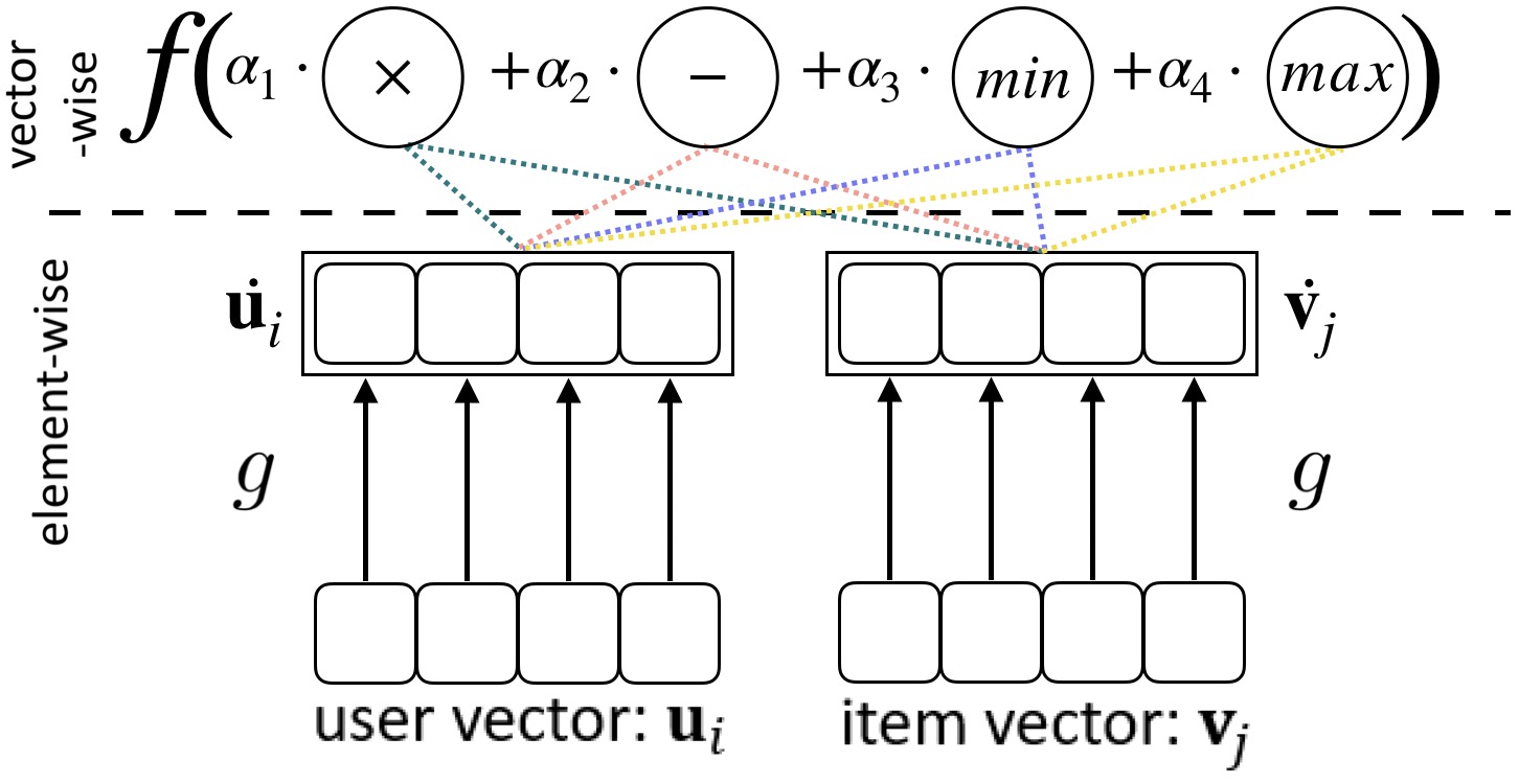
Figure 1. Representing the search space as a structured MLP. Vector-wise: standard linear algebra operations; element-wise: simple non-linear transformation.

3.3.2. Optimization by One-Shot Architecture Search

We present a stochastic algorithm (Algorithm 2) to optimize the structured MLP in Figure 1. The algorithm is inspired by NASP (Algorithm 1), in which the relaxation of operations is defined in (8). Again, we need to keep a discrete representation of the architecture, i.e., $\bar{\bm{\alpha}}$ at steps 3 and 8, but optimize a continuous architecture, i.e., $\bm{\alpha}$ at step 5. The difference is that we have extra continuous hyper-parameters $\bm{p}$ and $\bm{q}$ for element-wise nonlinear transformation here. They can still be updated by proximal steps (step 6), in which the closed-form solution is given by $\text{prox}_{\mathbb{I}(\|\cdot\|_{2}\leq 1)}(\bm{z})=\bm{z}/\|\bm{z}\|_{2}$ (Parikh and Boyd, 2013).

Algorithm 2 Searching Interaction Function (SIF) algorithm.

1:  Search space $\mathcal{F}$ represented by a structured MLP (Figure 1);

2:  while epoch $t=1,\cdots,T$ do

3:     Select one operation $\bar{\bm{\alpha}}=\text{prox}_{\mathcal{C}_{1}}(\bm{\alpha})$;

4:     sample a mini-batch from the validation data set;

5:     Update continuous $\bm{\alpha}$ for vector-wise operations

$$\bm{\alpha}=\text{prox}_{\mathcal{C}_{2}}(\bm{\alpha}-\eta\nabla_{\bar{\bm{\alpha}}}H(\bm{T},\bm{S}));$$

6:     Update element-wise transformation

$$\bm{p} =\text{prox}_{\mathbb{I}(\|\cdot\|_{2}\leq 1)}(\bm{p}-\eta\nabla_{\bm{p}}H(\bm{T},\bm{S})),$$

$$\bm{q} =\text{prox}_{\mathbb{I}(\|\cdot\|_{2}\leq 1)}(\bm{q}-\eta\nabla_{\bm{q}}H(\bm{T},\bm{S}));$$

7:     sample a mini-batch from the training data set;

8:     Obtain selected operation $\bar{\bm{\alpha}}=\text{prox}_{\mathcal{C}_{1}}(\bm{\alpha})$;

9:     Update training parameters $\bm{T}$ with gradients on $F_{\alpha}$;

10:  end while

11:  return  Searched interaction function (parameterized by $\bm{\alpha}$, $\bm{p}$ and $\bm{q}$, see (7) and (8)).

3.4. Extension to Tensor Data

As mentioned in Section 1, CF methods have also been used on tensor data. For example, low-rank matrix factorization is extended to tensor factorization, in which two decomposition formats, CP and Tucker (Kolda and Bader, 2009), have been popularly used. These two methods are also based on the inner product. Besides, the factorization machine (Rendle, 2012) is also recently extended to data cubes (Blondel et al., 2016). These motivate us to extend the proposed SIF algorithm to tensor data. In the sequel, we focus on the third-order tensor. Higher-order tensors can be handled in a similar way.

For tensors, we need to maintain three embedded vectors, $\bm{u}_{i}$, $\bm{v}_{j}$ and $\bm{s}_{l}$. First, we modify $f$ to take three vectors as input and output another vector. Subsequently, each candidate in search space (7) becomes $f=\mathcal{O}(\dot{\bm{u}}_{i},\dot{\bm{v}}_{j},\dot{\bm{s}}_{l})$, where $\dot{\bm{u}}_{i}$’s are obtained from element-wise MLP from $\bm{u}_{i}$ (and similarly for $\dot{\bm{v}}_{j}$ and $\dot{\bm{s}}_{l}$). However, $\mathcal{O}$ is no longer a single operation, as three vectors are involved. $\mathcal{O}$ enumerates all possible combinations from basic operations in the matrix case. For example, if only $\max$ and $\odot$ are allowed, then $\mathcal{O}$ contains $\max(\bm{u}_{i},\bm{v}_{j})\odot\bm{s}_{l}$, $\max(\max(\bm{u}_{i},\bm{v}_{j}),\bm{s}_{l})$, $\bm{u}_{i}\odot\max(\bm{v}_{j},\bm{s}_{l})$ and $\bm{u}_{i}\odot\bm{v}_{j}\odot\bm{s}_{l}$. With the above modifications, it is easy to see that the space can still be represented by a structured MLP similar to that in Figure 1. Moreover, the proposed Algorithm 2 can still be applied (see Appendix A.2). Note that the search space is much larger for tensor than matrix.

4. Empirical Study

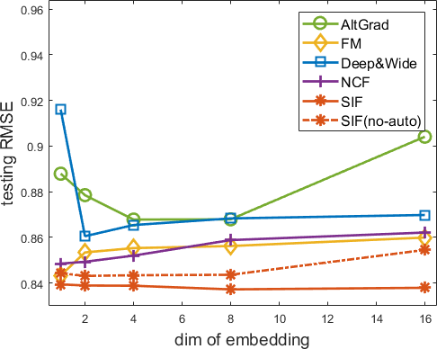
(a) MovieLens-100K.

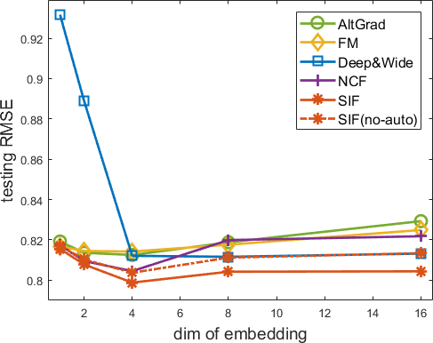
(b) MovieLens-1M.

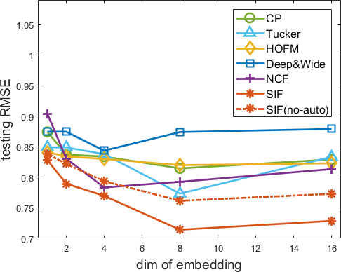
(c) Youtube.

Figure 2. Testing RMSEs of SIF and other CF approaches with different embedding dimensions.

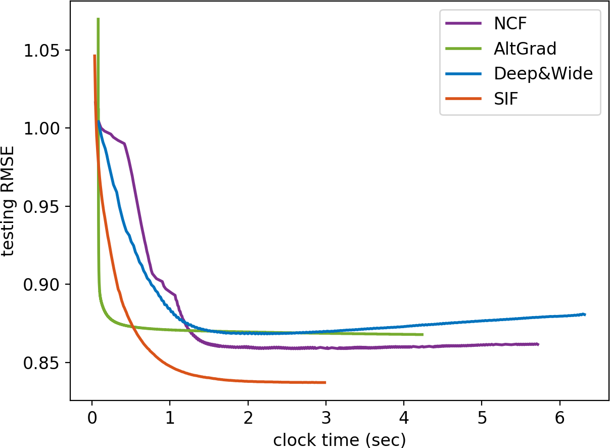
(a) MovieLens-100K.

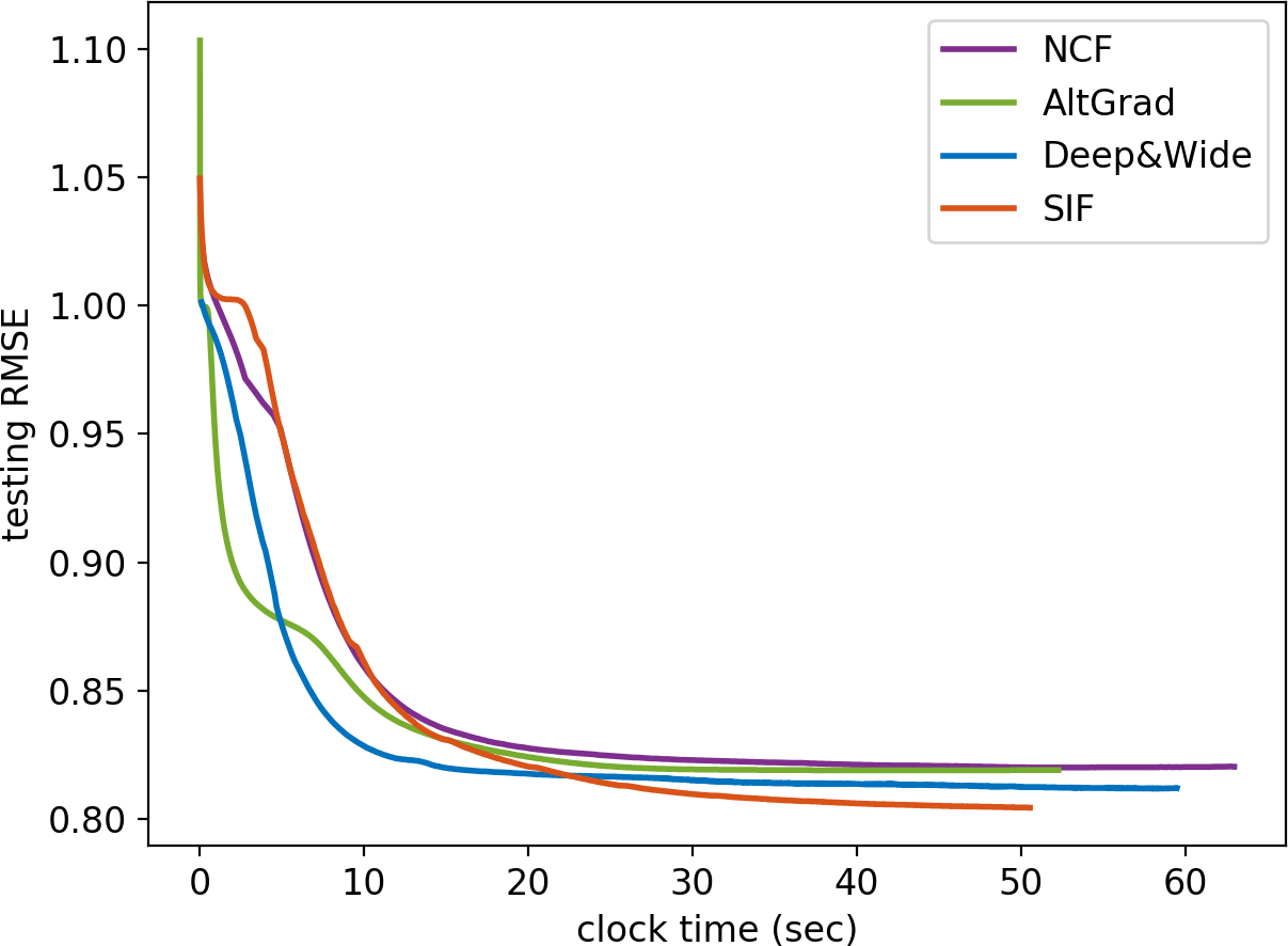
(b) MovieLens-1M.

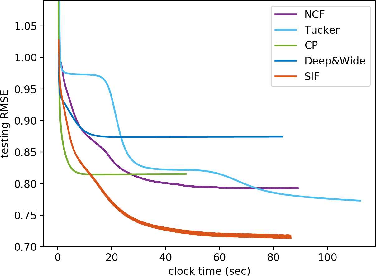
(c) Youtube.

Figure 3. Convergence of SIF (with searched IFC) and other CF methods with an embedded dimensionality of $8$. Algorithms FM and HOFM are not shown as their codes do not support a callback to record testing performance.

4.1. Experimental Setup

Two standard benchmark data sets (Table 2), MovieLens (matrix data) and Youtube (tensor data), are used in the experiments (Mnih and Salakhutdinov, 2008; Gemulla et al., 2011; Lei et al., 2009). Following (Wang et al., 2015; Yao and Kwok, 2018), we uniformly and randomly select 50% of the ratings for training, 25% for validation and the rest for testing. Note that since the size of the original Youtube dataset (Lei et al., 2009) is very large (approximate 27 times the size of MovieLens-1M), we sample a subset of it to test the performance (approximately the size of MovieLens-1M). We sample rows with interactions larger than 20.

Table 2. Data sets used in the experiments.

data set (matrix)		#users	#items	#ratings
MovieLens	100K	943	1,682	100,000
	1M	6,040	3,706	1,000,209

data set (tensor)	#rows	#columns	#depths	#nonzeros
Youtube	600	14,340	5	1,076,946

The task is to predict missing ratings given the training data. We use the square loss for both $\mathcal{M}$ and $\ell$. For performance evaluation, we use (i) the testing RMSE as in (Mnih and Salakhutdinov, 2008; Gemulla et al., 2011): $\text{RMSE}=[\frac{1}{|\tilde{\Omega}|}\sum\nolimits_{(i,j)\in\tilde{\Omega}}(\bm{w}^{\top}f(\bm{u}_{i},\bm{v}_{j})-\bm{O}_{ij})^{2}]^{\nicefrac{{1}}{{2}}},$ where $f$ is the operation chosen by the algorithm, and $\bm{w}$, $\bm{u}_{i}$’s and $\bm{v}_{j}$’s are parameters learned from the training data; and (ii) clock time (in seconds) as in (Baker et al., 2017; Liu et al., 2018). Except for IFCs, other hyper-parameters are all tuned with grid search on the validation set. Specifically, for all CF approaches, since the network architecture is already pre-defined, we tune the learning rate $lr$ and regularization coefficient $\lambda$ to obtain the best RMSE. We use the Adagrad (Duchi et al., 2010) optimizer for gradient-based updates. In our experiments, $lr$ is not sensitive, and we simply fix it to a small value. Furthermore, we utilize grid search to obtain $\lambda$ from $\left[0,10^{-6},5\times 10^{-6},10^{-5},5\times 10^{-5},10^{-4}\right]$. For the AutoML approaches, we use the same $lr$ to search for the architecture, and tune $\lambda$ using the same grid after the searched architecture is obtained.

4.2. Comparison with State-of-the-Art CF Approaches

In this section, we compare SIF with state-of-the-art CF approaches. On the matrix data sets, the following methods are compared: (i) Alternating gradient descent (“AltGrad”) (Koren, 2008): This is the most popular CF method, which is based on matrix factorization (i.e., inner product operation). Gradient descent is used for optimization; (ii) Factorization machine (“FM”) (Rendle, 2012): This extends linear regression with matrix factorization to capture second-order interactions among features; (iii) Deep&Wide (Cheng et al., 2016): This is a recent CF method. It first embeds discrete features and then concatenates them for prediction; (iv) Neural collaborative filtering (“NCF”) (He et al., 2017): This is another recent CF method which models the IFC by neural networks.

For tensor data, Deep&Wide and NCF can be easily extended to tensor data. Two types of popularly used low-rank factorization of tensor are used, i.e., “CP” and “Tucker” (Kolda and Bader, 2009), and gradient descent is used for optimization; “HOFM” (Blondel et al., 2016): a fast variant of FM, which can capture high-order interactions among features. Besides, we also compare with a variant of SIF (Algorithm 2), denoted SIF(no-auto), in which both the embedding parameter $\bm{T}$ and architecture parameter $\bm{S}$ are optimized using training data. Details on the implementation of each CF method and discussion of the other CF approaches are in Appendix A.4. All codes are implemented in PyTorch, and run on a GPU cluster with a Titan-XP GPU.

4.2.1. Effectiveness

Figure 2 shows the testing RMSEs. As the embedding dimension gets larger, all methods gradually overfit and the testing RMSEs get higher. SIF(no-auto) is slightly better than the other CF approaches, which demonstrates the expressiveness of the designed search space. However, it is worse than SIF. This shows that using the validation set can lead to better architectures. Moreover, with the searched IFCs, SIF consistently obtains lower testing RMSEs than the other CF approaches.

4.2.2. Convergence

If an IFC can better capture the interactions among user and item embeddings, it can also converge faster in terms of testing performance. Thus, we show the training efficiency of the searched interactions and human-designed CF methods in Figure 3. As can be seen, the searched IFC can be more efficient, which again shows superiority of searching IFCs from data.

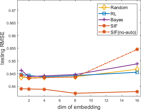
(a) MovieLens-100K.

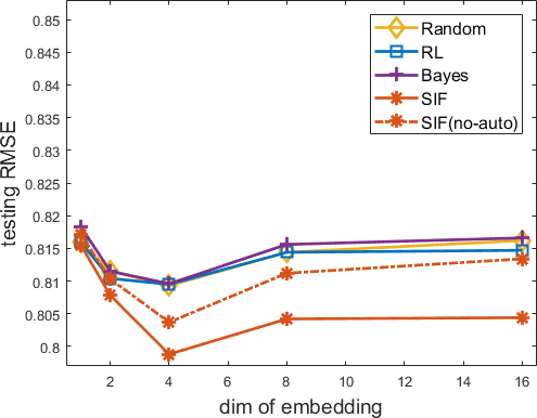
(b) MovieLens-1M.

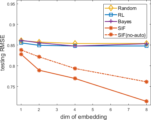
(c) Youtube.

Figure 4. Testing RMSEs of SIF and the other AutoML approaches, with different embedding dimensions. Gen-approx is not run on Youtube, as it is slow and the performance is inferior.

(a) MovieLens-100K.

(b) MovieLens-1M.

(c) Youtube.

Figure 5. Search efficiency of SIF and the other AutoML approaches (embedding dimension is $8$).

4.2.3. More Performance Metrics

As in (Kim et al., 2016; He et al., 2017, 2018), we report the metrics of “Hit at top” and “Normalized Discounted Cumulative Gain (NDCG) at top” on the MovieLens-100K data. Recall that the ratings are in the range $\{1,2,3,4,5\}$. We treat ratings that are equal to five as positive, and the others as negative. Results are shown in Table 3. The comparison between SIF and SIF(no-auto) shows that using the validation set can lead to better architectures. Besides, SIF is much better than the other methods in terms of both Hit@K and NDCG@K, and the relative improvements are larger than that on RMSE.

Table 3. Hit-at-top (H@K) and NDCG-at-top (N@K) on MovieLens-100K.

	RMSE	H@5	H@10	N@5	N@10
Altgrad	0.867	0.267	0.377	0.156	0.220
FM	0.845	0.286	0.391	0.176	0.249
Deep&Wide	0.861	0.273	0.378	0.163	0.227
NCF	0.851	0.279	0.386	0.172	0.236
SIF(no-auto)	0.846	0.284	0.390	0.175	0.250
SIF	0.839	0.295	0.405	0.190	0.259

4.3. Comparison with State-of-the-Art AutoML Search Algorithms

In this section, we compare with the following popular AutoML approaches: (i) “Random”: Random search (Bergstra and Bengio, 2012) is used. Both operations and weights (for the small and fixed MLP) in the designed search space (in Section 3.2) are uniformly and randomly set; (ii) “RL”: Following (Zoph and Le, 2017), we use reinforcement learning (Sutton and Barto, 1998) to search the designed space; (iii) “Bayes”: The designed search space is optimized by HyperOpt (Bergstra et al., 2015), a popular Bayesian optimization approach for hyperparameter tuning; and (iv) “SIF”: The proposed Algorithm 2; and (v) “SIF(no-auto)”: A variant of SIF in which parameter $\bm{S}$ for the IFCs are also optimized with training data. More details on the implementations and discussion of the other AutoML approaches are in Appendix A.5.

4.3.1. Effectiveness

Figure 4 shows the testing RMSEs of the various AutoML approaches. Experiments on MovieLens-10M are not performed as the other baseline methods are very slow (Figure 5). SIF(no-auto) is worse than SIF as the IFCs are searched purely based on the training set. Among all the methods tested, the proposed SIF is the best. It can find good IFCs, leading to lower testing RMSEs than the other methods for the various embedding dimensions.

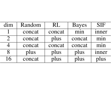
(a) Operations (vector-wise).

(b) Nonlinear transformation (element-wise).

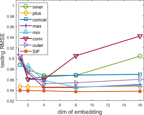
(c) Performance of each single operation.

Figure 6. (a) operations identified by various search algorithms on MovienLens-100K; (b) Searched IFCs on MovienLens-100K when embedding dimension is $8$; (c) Performance for SIF and each single operation on MovieLens-100K.

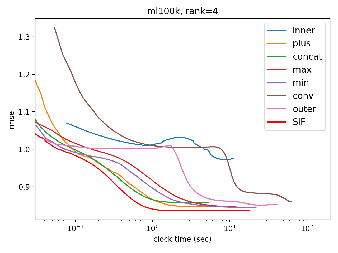
(a) embedding dimension = 4.

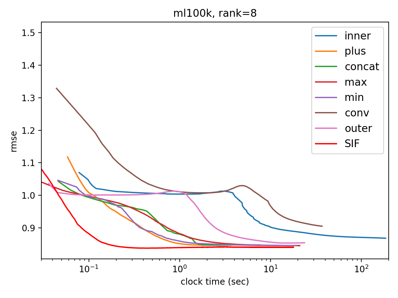
(b) embedding dimension = 8.

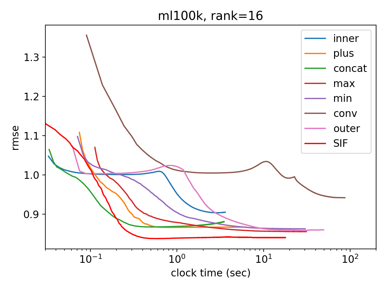
(c) embedding dimension = 16.

Figure 7. Convergence of various single operations on MovieLens-100K, with different embedding dimensions.

4.3.2. Search Efficiency

In this section, we take the $k$ architectures with top validation performance, re-train, and then report their average RMSE on the testing set in Figure 5. As can be seen, all algorithms run slower on Youtube, as the search space for tensor data is larger than that for matrix data. Besides, SIF is much faster than all the other methods and has lower testing RMSEs. The gap is larger on the Youtube data set. Finally, Table 4 reports the time spent on the search and fine-tuning. As can be seen, the time taken by SIF is less than five times of those of the other non-autoML-based methods.

Table 4. Clock time (in seconds) taken by SIF and the other CF approaches (embedding dimension is $8$).

	AltGrad	FM	Deep&Wide	NCF	SIF	SIF(no-auto)
MovieLens-100K	25.4	43.1	37.9	34.3	159.8	73.4
MovieLens-1M	313.7	324.3	357.0	374.9	745.3	348.7

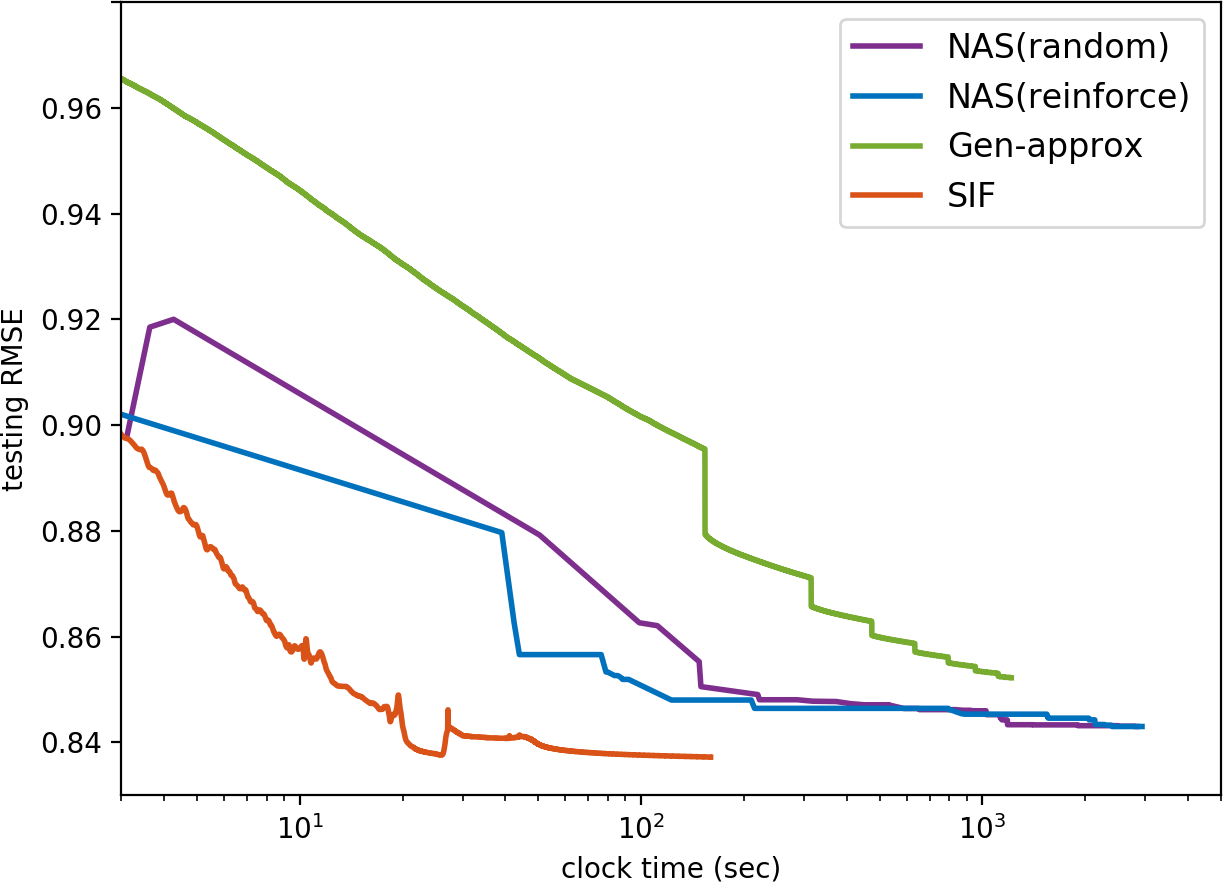
(a) MovieLens-100K.

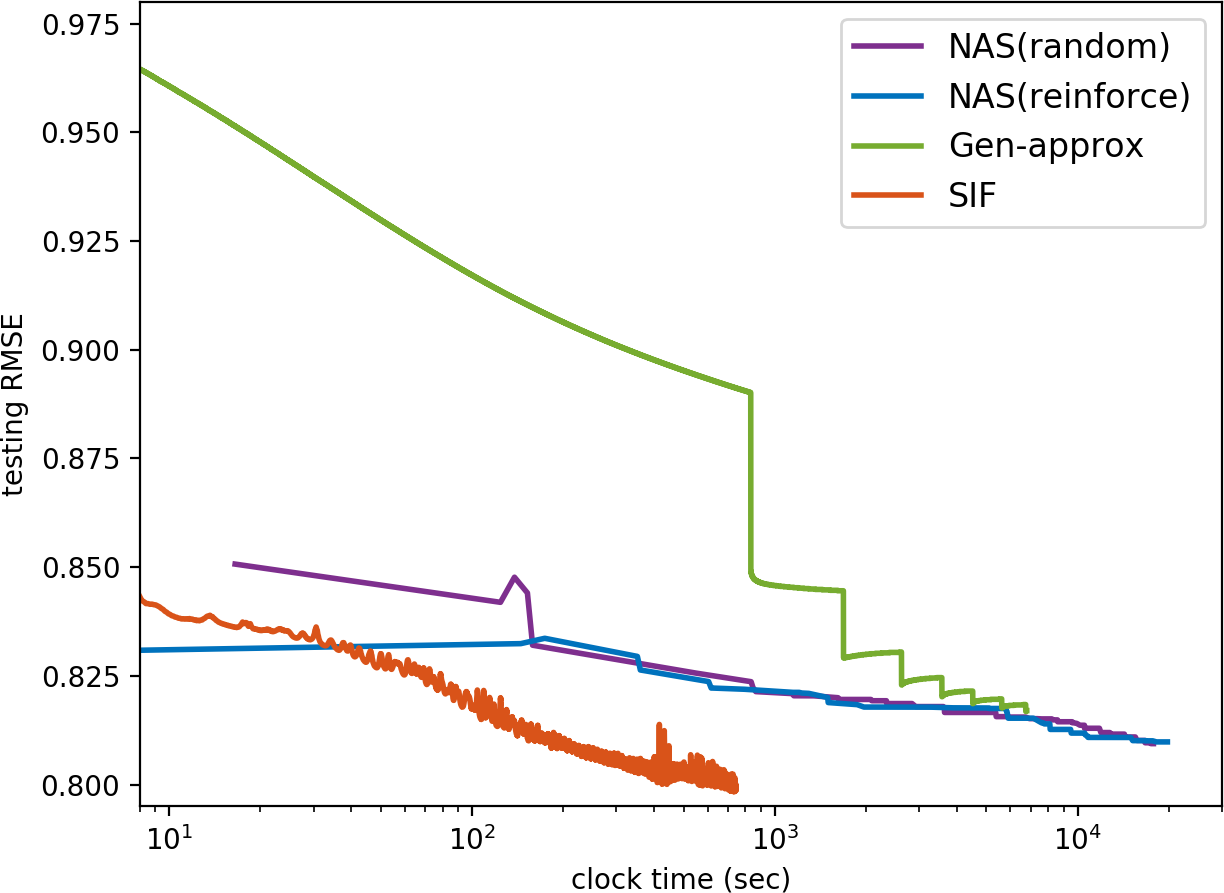
(b) MovieLens-1M.

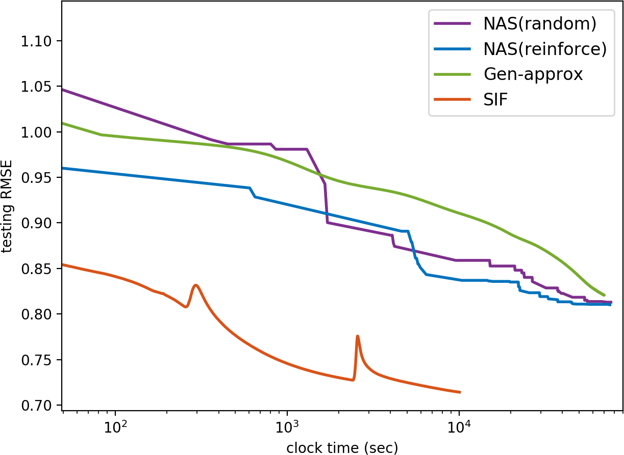
(c) Youtube.

Figure 8. Comparison on different search space designs (embedding dimension is 8).

4.4. Interaction Functions (IFCs) Obtained

To understand why a lower RMSE can be achieved by the proposed method, we show the IFCs obtained by the various AutoML methods on MovieLens-100K. Figure 6(a) shows the vector-wise operations obtained. As can be seen, Random, RL, Bayes and SIF select different operations in general. Figure 6(b) shows the searched nonlinear transformation for each element. We can see that SIF can find more complex transformations than the others.

To further demonstrate the need of AutoML and effectiveness of SIF, we show the performance of each single operation in Figure 6(c). It can be seen that while some operations can be better than others (e.g., plus is better than conv), there is no clear winner among all operations. The best operation may depend on the embedding dimension as well. These verify the need for AutoML. Figure 7 shows the testing RMSEs of all single operations. We can see that SIF consistently achieves lower testing RMSEs than all single operations and converges faster. Note that SIF in Figure 6(a) may not select the best single operation in Figure 6(c), due to the learned nonlinear transformation (Figure 6(b)).

Table 5. Results on MovieLens-100K with $k$ selected operations in SIF.

	embedding dimension = 4		embedding dimension = 8
$k$	RMSE	operator	RMSE	operator
1	0.8448	concat	0.8450	max
2	0.8435	concat, max	0.8440	max, plus
3	0.8442	concat, max, multiply	0.8432	max, plus, concat
4	0.8433	concat, max, multiply, plus	0.8437	max, plus, concat, min
5	0.8432	concat, max, multiply, plus, min	0.8431	max, plus, concat, min, multiply

Table 6. Testing RMSE on MovieLens-100K with different activation functions and number of hidden units in the MLP for element-wise transformation.

embedding	activation	number of hidden units
dimension	function	1	5	10	15	20
	relu	0.8437	0.8388	0.8385	0.8389	0.8396
4	sigmoid	0.8440	0.8391	0.8390	0.8395	0.8399
	tanh	0.8439	0.8991	0.8389	0.8393	0.8401
	relu	0.8385	0.8372	0.8370	0.8371	0.8374
8	sigmoid	0.8382	0.8375	0.8377	0.8376	0.8378
	tanh	0.8386	0.8376	0.8373	0.8375	0.8377

4.5. Ablation Study

In this section, we perform ablation study on different parts of the proposed AutoML method.

4.5.1. Different Search Spaces

First, we show the superiority of search space used in SIF by comparing with the following approaches:

• Using a MLP as a general approximator (“Gen-approx”), as described in Section 3.2, to approximate the search space is also compared. The MLP is updated with stochastic gradient descent (Bengio, 2000) using the validation set. Since searching network architectures is expensive (Zoph and Le, 2017; Zoph et al., 2017), the MLP structure is fixed for Gen-approx (see Appendix A.1).

• Standard NAS approach, using MLP to approximate the IFC $f$. The MLP is optimized with the training data, while its architecture is searched with the validation set. Two search algorithms are considered: (i) random search (denoted ‘‘NAS(random)”) (Bergstra and Bengio, 2012); (ii) reinforcement learning (denoted “NAS(reinforce)”) (Zoph and Le, 2017).

The above are general search spaces, and are much larger than the one designed for SIF.

Figure 8 shows the convergence of testing RMSE for the various methods. As can be seen, these general approximation methods are hard to be searched and thus much slower than SIF. The proposed search space in Section 3.2 is not only compact, but also allows efficient one-shot search as discussed in Section 3.3.

4.5.2. Allowing More Operations

In Algorithm 2, we only allow one operation to be selected. Here, we allow more operations by changing $\mathcal{C}_{1}$ to $\mathcal{C}_{k}=\left\{\bm{\alpha}\,|\,\|\bm{\alpha}\|_{0}=k\right\}$, where $k\in\{1,2,\dots,5\}$. Results are shown in Table 5. As can be seen, the testing RMSE gets slightly smaller. However, the model complexity and prediction time grow linearly with $k$, and so can become significantly larger.

4.5.3. Element-wise Transformation

Recall that in Section 3.2, we use a small MLP to approximate an arbitrary element-wise transformation. In this experiment, we vary the number of hidden units and type of activation function in this MLP. Results on the testing RMSE are shown in Table 6. As can be seen, once the number of hidden units is large enough (i.e., $\geq 5$ here), the performance is stable with different number of activation functions. This demonstrates the robustness of our design in the search space.

4.5.4. Changing Predictor to MLP

In (5), we used a linear predictor. Here, we study whether using a more complicated predictor can further boost learning performance. A standard three-layer MLP with 10 hidden units is used. Results are shown in Table 7. As can be seen, using a more complex predictor can lead to lower testing RMSE when the embedding dimension is 4, 8, and 16. However, the lowest testing RMSE is still achieved by the linear predictor with an embedding dimension of 2. This demonstrates that the proposed SIF can achieve the desired performance, and designing a proper predictor is not an easy task.

Table 7. Testing RMSE on MovieLens-100K with MLP and linear predictor in (5).

	MLP		linear
embedding dim	RMSE	operator	RMSE	operator
2	0.8437	concat	0.8389	min
4	0.8424	concat	0.8429	min
8	0.8407	plus	0.8468	inner
16	0.8413	multiply	0.8467	plus

5. Conclusion

In this paper, we propose an AutoML approach to search for interaction functions in CF. The keys for its success are (i) an expressive search space, (ii) a continuous representation of the space, and (iii) an efficient algorithm which can jointly search interaction functions and update embedding vectors in a stochastic manner. Experimental results demonstrate that the proposed method is much more efficient than popular AutoML approaches, and also obtains much better learning performance than human-designed CF approaches.

Appendix A Appendix

A.1. General Search Space

As in Figure 1 and (7), we can take a three-layer MLP as $\mathcal{F}$, which is guaranteed to approximate any given function with enough hidden units (Raghu et al., 2017). We concatenate $\bm{u}_{i}$ and $\bm{v}_{j}$ as input to MLP. To ensure the approximation ability of MLP, we set the number of hidden units to be double that of the input size, and use the sigmoid function as the activation function. The final output is a vector of the same dimension as $\bm{u}_{i}$.

A.2. Tensor Data

Following Section 3.4, the proposed Algorithm 2 can be extended to tensor data. If only the times and max operations are allowed, the search space can be represented as in Figure 9, which is similar to Figure 1. Note that two possible operations are chosen, so the search space for tensor data is much larger than that for matrix data ($O(K)$ vs $O(K^{2})$, where $K$ is the number of operations).

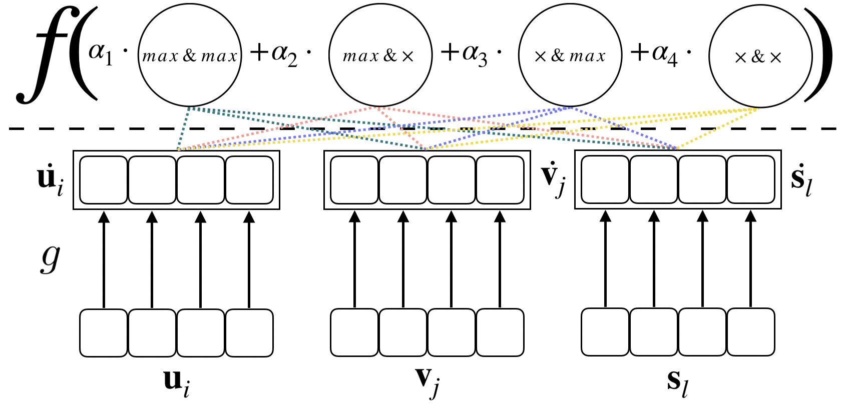
Figure 9. Representation of the search space for tensor data.

A.3. Proofs of Proposition 3.1

Proof.

Taking $f$ as the inner product function as an example. Let $\bm{A}=\{\bm{U},\bm{V},\bm{w}\}\neq\bm{0}$ be an optimal point of $F$, then $F(\bm{A})=\sum\nolimits_{(i,j)\in\Omega}\ell(\bm{w}^{\top}f(\bm{u}_{i},\bm{v}_{j}),\bm{O}_{ij})^{2}+\nicefrac{{\lambda}}{{2}}\|\bm{U}\|_{F}^{2}+\nicefrac{{\lambda}}{{2}}\|\bm{V}\|_{F}^{2}$. We construct another $\bm{A}^{\prime}=\{\beta\bm{U},\beta\bm{V},\nicefrac{{1}}{{\beta^{2}}}\bm{w}\}$ with $\beta\in(0,1)$, then $F\left(\bm{A}^{\prime}\right)=\sum_{(i,j)\in\Omega}\ell(\bm{w}^{\top}f(\bm{u}_{i},\bm{v}_{j}),\bm{O}_{ij})^{2}+\nicefrac{{\lambda\beta^{2}}}{{2}}\|\bm{U}\|_{F}^{2}+\nicefrac{{\lambda\beta^{2}}}{{2}}\|\bm{V}\|_{F}^{2}<F(\bm{A})$, which violates the assumption that $\bm{A}\neq\bm{0}$ is an optimal solution. The same holds for $f$ being other operations in Table1. ∎

A.4. Implementation: CF Approaches

AltGrad: It is the traditional way to perform collaborative filtering. We first apply an element-wise product of the user and item embedding and then feed the outputs into a linear predictor. In other word, AltGrad is equivalent to using the single inner operation in our searching space.

Factorization Machine: For the matrix case, we directly utilize the implementation from pyFM , noting that pyFM is difficult to run on GPU so it is not comparable to other methods when it comes to training time. For tensor case (HOFM), we use the implementation from tffm , which can be easily accelerated by GPU since tffm is implemented with tensorflow.

Deep & Wide: We implement Deep & Wide by employing a two layer MLP with ReLU as the non-linear function on the concatenation of all potential embeddings.

NCF: Neural collaborative filtering is flexible to stack many layers and become very deep as well as learn separate embeddings for GMF and MLP. But this paper focuses on the interaction function, and also to ensure similar computational complexity, we implement NCF by combining generalized matrix factorization (GMF) with a one-layer multi-layer perceptron (MLP). Noting that our method also supports deep models by changing the last linear predictor to a deep MLP.

CP: Similar to AltGrad, CP first combines three embeddings by an element-wise product, then the prediction is carried out through a linear predictor.

Tucker: Tucker has high computation complexity since it has a 3-D weight to perform Tucker decomposition. We implement this method by sequentially applying tensor product along all three dimensions and then feed the result into a linear predictor.

Others: Note that, CML (Hsieh et al., 2017; Zhang et al., 2016), ConvMF (Kim et al., 2016) and ConvNCF (He et al., 2018) are not included, since their CF tasks are different and codes are not available. Instead, interaction functions they introduced (Table 1) are studied in Section 4.4.

A.5. Implementation: AutoML Approaches

General Approximator: As in AutoML literature, the search space needs to be carefully designed, it cannot be too large (hard to be searched) nor too small (poor performance). In the experiments, we use MLP structure in Appendix A.1. The standard approach to optimize MLP is gradient descent on hyper-parameters (please see (Bergstra and Bengio, 2012)). However, it is very slow — in order to perform one gradient descent on MLP, we need to finish the training of CF model, which is one full model training on the training dataset. MLP needs many iterations to converge, and thus to train a good MLP, we need many times of full model training. This makes Gen-Approx very slow.

Random: In this baseline, architecture is randomly generated including the weights $\bm{p}$, $\bm{q}$ for element-wise MLP and the interaction function $f$ in every epoch. Every weights of $\bm{p}$, $\bm{q}$ is restricted within $[-3.0,3.0]$. We then report the best RMSE achieved after a fixed number of architectures are sampled.

Bayes: We directly use the source code from hyperopt (Bergstra et al., 2015) to perform Bayesian optimization. Every single weight of $\bm{p}$, $\bm{q}$ is designed as a uniform space ranging from -3.0 to 3.0. This continuous space along with the discrete space of interaction function is then jointly optimized, we report the best RMSE until a fixed number of evaluations are achieved.

Reinforcement Learning: Following (Zoph and Le, 2017), we utilize a controller to generate the architecture including $\bm{p}$, $\bm{q}$ and the interaction function $f$ to combine all potential embeddings. The difference lies in that the searching space in our setting is a combined continuous ($\bm{p}$, $\bm{q}$) and discrete (interaction function) space, so deterministic policy gradient is utilized (Silver et al., 2014; Lillicrap et al., 2015) to train the controller. We employ a recurrent neural network to act as the controller in order to be flexible to both matrix and tensor. The controller is then trained via policy gradient where the reward is $\nicefrac{{1}}{{\text{RMSE}}}$ of the generated architecture on the validation set. At convergence, a neural network is built following the output of the controller and the RMSE on test set is recorded.

Others: SMAC (Feurer et al., 2015) is not compared as it cannot be run on our GPU cluster and HyperOpt has comparable performance (Kandasamy et al., 2019). Genetic algorithms (Hutter et al., 2018) are also not compared as they need special designs to fit into our search space, and is inferior to RL and random search (Zoph and Le, 2017; Liu et al., 2018).

References

- (1)
- Aggarwal (2017) C. Aggarwal. 2017. Recommender systems: the textbook. Springer.
- Baker et al. (2017) B. Baker, O. Gupta, N. Naik, and R. Raskar. 2017. Designing Neural Network Architectures using Reinforcement Learning. In International Conference on Learning Representations.
- Bender et al. (2018) Gabriel Bender, Pieter-Jan Kindermans, Barret Zoph, Vijay Vasudevan, and Quoc Le. 2018. Understanding and simplifying one-shot architecture search. In International Conference on Machine Learning. 549–558.
- Bengio (2000) Y. Bengio. 2000. Gradient-based optimization of hyperparameters. Neural Computation 12, 8 (2000), 1889–1900.
- Bergstra and Bengio (2012) J. Bergstra and Y. Bengio. 2012. Random search for hyper-parameter optimization. Journal of Machine Learning Research 13, Feb (2012), 281–305.
- Bergstra et al. (2015) J. Bergstra, B. Komer, C. Eliasmith, D. Yamins, and D. Cox. 2015. Hyperopt: a python library for model selection and hyperparameter optimization. Computational Science & Discovery 8, 1 (2015), 014008.
- Blondel et al. (2016) M. Blondel, A. Fujino, N. Ueda, and M. Ishihata. 2016. Higher-order factorization machines. In Neural Information Processing Systems. 3351–3359.
- Candès and Recht (2009) E. Candès and B. Recht. 2009. Exact matrix completion via convex optimization. Foundations of Computational mathematics 9, 6 (2009), 717.
- Cheng et al. (2016) H.-T. Cheng, L. Koc, J. Harmsen, T. Shaked, T. Chandra, H. Aradhye, G. Anderson, G. Corrado, W. Chai, and M. Ispir. 2016. Wide & deep learning for recommender systems. Technical Report. Recsys Workshop.
- Colson et al. (2007) B. Colson, P. Marcotte, and G. Savard. 2007. An overview of bilevel optimization. Annals of Operations Research 153, 1 (2007), 235–256.
- Dacrema et al. (2019) M. F. Dacrema, P. Cremonesi, and D. Jannach. 2019. Are we really making much progress? A worrying analysis of recent neural recommendation approaches. In ACM Recommender Systems. ACM, 101–109.
- Duchi et al. (2010) J. Duchi, E. Hazan, and Y. Singer. 2010. Adaptive Subgradient Methods for Online Learning and Stochastic Optimization. Journal of Machine Learning Research (2010).
- Feurer et al. (2015) M. Feurer, A. Klein, K. Eggensperger, J. Springenberg, M. Blum, and F. Hutter. 2015. Efficient and robust automated machine learning. In Neural Information Processing Systems. 2962–2970.
- Gemulla et al. (2011) R. Gemulla, E. Nijkamp, P. Haas, and Y. Sismanis. 2011. Large-scale matrix factorization with distributed stochastic gradient descent. In ACM SIGKDD Conference on Knowledge Discovery and Data Mining. 69–77.
- Goodfellow et al. (2016) I. Goodfellow, Y. Bengio, and A. Courville. 2016. Deep learning. MIT press.
- He et al. (2018) X. He, X. Du, X. Wang, F. Tian, J. Tang, and T.-S. Chua. 2018. Outer product-based neural collaborative filtering. In International Joint Conferences on Artificial Intelligence. 2227–2233.
- He et al. (2017) X. He, L. Liao, H. Zhang, L. Nie, X. Hu, and T.-S. Chua. 2017. Neural Collaborative Filtering. The Web Conference (2017).
- Herlocker et al. (1999) J. Herlocker, J. Konstan, A. Borchers, and J. Riedl. 1999. An algorithmic framework for performing collaborative filtering. In ACM SIGIR Conference on Research and Development in Information Retrieval. 230–237.
- Hsieh et al. (2017) C.-K. Hsieh, L. Yang, Y. Cui, T.-Y. Lin, S. Belongie, and D. Estrin. 2017. Collaborative metric learning. In The Web Conference. International World Wide Web Conferences Steering Committee, 193–201.
- Hutter et al. (2018) F. Hutter, L. Kotthoff, and J. Vanschoren (Eds.). 2018. Automated Machine Learning: Methods, Systems, Challenges. Springer.
- Ji et al. (2010) H. Ji, C. Liu, Z. Shen, and Y. Xu. 2010. Robust video denoising using low rank matrix completion. In IEEE Conference on Computer Vision and Pattern Recognition. 1791–1798.
- Kandasamy et al. (2019) K. Kandasamy, K. Vysyaraju, W. Neiswanger, B. Paria, C. Collins, J. Schneider, B. Poczos, and E. Xing. 2019. Tuning Hyperparameters without Grad Students: Scalable and Robust Bayesian Optimisation with Dragonfly. Technical Report. arXiv preprint.
- Karatzoglou et al. (2010) A. Karatzoglou, X. Amatriain, L. Baltrunas, and N. Oliver. 2010. Multiverse recommendation: n-dimensional tensor factorization for context-aware collaborative filtering. In ACM Recommender Systems. 79–86.
- Kim et al. (2016) D. Kim, C. Park, J. Oh, S. Lee, and H. Yu. 2016. Convolutional matrix factorization for document context-aware recommendation. In ACM Recommender Systems. 233–240.
- Kim and Leskovec (2011) M. Kim and J. Leskovec. 2011. The network completion problem: Inferring missing nodes and edges in networks. In SIAM International Conference on Data Mining. SIAM, 47–58.
- Kolda and Bader (2009) T.G. Kolda and B. Bader. 2009. Tensor decompositions and applications. SIAM Rev. 51, 3 (2009), 455–500.
- Koren (2008) Y. Koren. 2008. Factorization meets the neighborhood: a multifaceted collaborative filtering model. In ACM SIGKDD Conference on Knowledge Discovery and Data Mining.
- Lei et al. (2009) T. Lei, X. Wang, and H. Liu. 2009. Uncoverning groups via heterogeneous interaction analysis. In IEEE International Conference on Data Mining. 503–512.
- Lillicrap et al. (2015) T. Lillicrap, J. Hunt, A. Pritzel, N. Heess, T. Erez, Y. Tassa, D. Silver, and D. Wierstra. 2015. Continuous control with deep reinforcement learning. Technical Report. arXiv.
- Liu et al. (2018) H. Liu, K. Simonyan, and Y. Yang. 2018. DARTS: Differentiable architecture search. In International Conference on Learning Representations.
- Mnih and Salakhutdinov (2008) A. Mnih and R. Salakhutdinov. 2008. Probabilistic matrix factorization. In Neural Information Processing Systems. 1257–1264.
- Parikh and Boyd (2013) N. Parikh and S.P. Boyd. 2013. Proximal algorithms. Foundations and Trends in Optimization 1, 3 (2013), 123–231.
- Raghu et al. (2017) M. Raghu, B. Poole, J. Kleinberg, S. Ganguli, and J. Dickstein. 2017. On the expressive power of deep neural networks. In International Conference on Machine Learning. 2847–2854.
- Recht et al. (2010) B. Recht, M. Fazel, and P. Parrilo. 2010. Guaranteed minimum-rank solutions of linear matrix equations via nuclear norm minimization. SIAM review 52, 3 (2010), 471–501.
- Rendle (2012) S. Rendle. 2012. Factorization machines with LibFM. ACM Transactions on Intelligent Systems and Technology 3, 3 (2012), 57.
- Silver et al. (2014) D. Silver, G. Lever, N. Heess, T. Degris, D. Wierstra, and M. Riedmiller. 2014. Deterministic Policy Gradient Algorithms. In International Conference on Machine Learning. I–387–I–395.
- Su and Khoshgoftaar (2009) X. Su and T. Khoshgoftaar. 2009. A survey of collaborative filtering techniques. Advances in Artificial Intelligence 2009 (2009).
- Sutton and Barto (1998) R. Sutton and A. Barto. 1998. Reinforcement learning: An introduction. MIT press.
- Wang and Blei (2011) C. Wang and D. M Blei. 2011. Collaborative topic modeling for recommending scientific articles. In ACM SIGKDD Conference on Knowledge Discovery and Data Mining. ACM, 448–456.
- Wang et al. (2015) Z. Wang, M.-J. Lai, Z. Lu, W. Fan, H. Davulcu, and J. Ye. 2015. Orthogonal rank-one matrix pursuit for low rank matrix completion. SIAM Journal on Scientific Computing 37, 1 (2015), A488–A514.
- Xie et al. (2018) S. Xie, H. Zheng, C. Liu, and L. Lin. 2018. SNAS: stochastic neural architecture search. In International Conference on Learning Representations.
- Xue et al. (2017) H.-J. Xue, X. Dai, J. Zhang, S. Huang, and J. Chen. 2017. Deep Matrix Factorization Models for Recommender Systems. In International Joint Conferences on Artificial Intelligence.
- Yao and Kwok (2018) Q. Yao and J. Kwok. 2018. Accelerated and inexact soft-impute for large-scale matrix and tensor completion. IEEE Transactions on Knowledge and Data Engineering (2018).
- Yao and Wang (2018) Q. Yao and M. Wang. 2018. Taking Human out of Learning Applications: A Survey on Automated Machine Learning. Technical Report. arXiv preprint arXiv:1810.13306.
- Yao et al. (2020) Q. Yao, J. Xu, W.-W. Tu, and Z. Zhu. 2020. Efficient Neural Architecture Search via Proximal Iterations. In AAAI Conference on Artificial Intelligence.
- Zhang et al. (2016) F. Zhang, J. Yuan, D. Lian, X. Xie, and W.-Y. Ma. 2016. Collaborative Knowledge Base Embedding for Recommender Systems. In ACM SIGKDD Conference on Knowledge Discovery and Data Mining.
- Zhang et al. (2019) Y. Zhang, Q. Yao, W. Dai, and L. Chen. 2019. AutoKGE: Searching Scoring Functions for Knowledge Graph Embedding. Technical Report. arXiv preprint arXiv:1902.07638.
- Zoph and Le (2017) B. Zoph and Q. Le. 2017. Neural architecture search with reinforcement learning. In International Conference on Learning Representations.
- Zoph et al. (2017) B. Zoph, V. Vasudevan, J. Shlens, and Q. Le. 2017. Learning Transferable Architectures for Scalable Image Recognition. In IEEE Conference on Computer Vision and Pattern Recognition.