Ground-state cooling of an magnomechanical resonator induced by magnetic damping

Abstract

Quantum manipulation of mechanical resonators has been widely applied in fundamental physics and quantum information processing. Among them, cooling the mechanical system to its quantum ground state is regarded as a key step. In this work, we propose a scheme which one can realize ground-state cooling of resonator in a cavity magnomechanical system. The system consists of a microwave cavity and a small ferromagnetic sphere, in which phonon-magnon coupling and cavity photon-magnon coupling can be achieved via magnetostrictive interaction and magnetic dipole interaction, respectively. After adiabatically eliminating the cavity mode, an effective Hamiltonian which consists of magnon and mechanical modes is obtained. Within experimentally feasible parameters, we demonstrate that the ground-state cooling of the magnomechanical resonator can be achieved by extra magnetic damping. Unlike optomechanical cooling, magnomechanical interaction is utilized to realize the cooling of resonators. We further illustrate the ground-state cooling can be effectively controlled by the external magnetic field.

I Introduction

In recent years, the ferrimagnetic systems has attracted considerable interest, which can realize the strong light-matter interactions. Among them, the cavity-magnon systems developed from cavity quantum electrodynamics (QED) systems have been theoretically proposed and experimentally demonstrated in the past few years p0 ; p1 ; p2 ; p3 ; p4 ; i1 ; i2 ; i3 ; i4 ; i5 ; i51 ; i52 ; i53 ; g9 . A highly polished single-crystal yttrium iron garnet (YIG) sphere is placed in a 3-dimensional rectangular microwave cavity. Due to YIG sphere’s high spin density and low damping rate, the Kittel mode k15 (the ferromagnetic resonance mode) in it can stronglyi3 ; i6 ; i7 and even possibly ultrastrong i8 couple to the microwave cavity photons. Compared with previous quantum systems, the cavity-magnon system has the merits of high tunability and good coherence. This system has shown its extensive application prospects, including the bistability of cavity magnon polaritons k6 , the higher-order exceptional point k211 , magnon Kerr effect in strong coupling regime k2 , the light transmission k23 and other researches k24 ; k25 ; k5 ; k7 ; k21 .

Cavity optomechanics is a rapidly developing research area for exploring the radiation-pressure-mediated interaction between photons and mechanical systems k00 ; k000 ; k001 ; k002 ; k003 ; k004 ; k005 ; k006 ; k007 . In the view of these important results, it is natural to investigate the magnon-phonon interaction in YIG spheres and their quantum characteristics. So far, some approaches on cavity magnomechanical systems have been proposed k0 ; k1 ; k151 ; k16 ; k26 , where the interaction between magnons and phonons can be achieved by the magnetostrictive force (radiation-pressure-like). The varying magnetization caused by the excitation of the magnons in the YIG sphere results in the geometric deformation of the surface, introducing the coupling between magnon mode and phonon mode. Generally speaking, the magnomechanical state-swap interaction is much small in experiments and can be neglected. However, it can be significantly enhanced by driving the magnon mode with a strong red-detuned microwave field k6 ; k0 .

The cooling of the systems to theirs ground states is a prerequisite for observing the signature of quantum effects in mechanical systems k27 ; k28 ; k29 ; k30 ; k31 ; k32 ; k33 ; k34 ; k35 ; k36 ; g5 . Accordingly, preparing mechanical quantum states free of thermal noise is a crucial goal in various mechanical systems. Among them, the cavity magnomechanical system has attracted much interest because of its intrinsic great tunability, low loss, and promising integration with electromechanical elements. In addition, the cavity magnomechanical system provides a promising platform for the study of macroscopic quantum phenomena.

Here, we explore theoretically the ground-state cooling of the magnomechanical resonator with experimentally reachable parameters. The system consists of a YIG sphere placed in a low-Q microwave cavity, and an uniform external bias magnetic field. Base on the highly dissipative cavity mode, the system is effectively transformed into a two-mode system, which is composed of a magnon mode and a mechanical mode. Then we give the expression of the final phonon number in the full quantum theory, it illustrates that the magnon mode can be utilized to cool the resonator to its ground-state. In order to achieve better cooling effect, a drive magnetic field is introduced to enhance the magnon-phonon coupling. In addition, the ground state cooling can be well controlled by adjusting the external magnetic field without changing other parameters, which provides an additional degree of freedom.

The structure of the paper is as follows. In Sec. II, we frist establish a physical model and give the linearized Hamiltonian. Then, by assuming the cavity mode is highly dissipative, the effective Hamiltonian by adiabatically eliminating optical mode is given. We also show the equations of motion. In Sec. III, we give the analytic expression of extra magnetic damping for the magnomechanical resonator, then the final phonon number is studied. We also find the ground-state cooling of an magnomechanical resonator can be achieved with the experimentally feasible parameters. The effects of external magnetic field on the cooling are also studied. Finally, we make a conclusion based on the results obtained in sec. IV.

II Model and effective Hamiltonian

We utilize a hybrid system as shown in Fig. 1(a), which consists a microwave cavity and a small sphere (a highly polished single-crystal YIG sphere of diameter $1mm$ is used in k2 ). The YIG sphere is placed near the maximum microwave magnetic field of the cavity mode, and we add an adjustable external magnetic field $H$ in $z$-axis, which establishes the magnon-photon coupling k2 ; k6 , and the rate of coupling can be tuned by the position of YIG sphere in the cavity. The adjusting range of bias magnetic field $H$ is between $0$ and $1T$ k2 .

Because of the magnetostrictive effect, YIG sphere can be used as an excellent mechanical resonator. Therefore, the term of coupling between magnons and phonons can be introduced into Hamiltonian of our system as mentioned in k1 . Based on it, we have the vibrational mode (phonons) of the sphere.

There are three modes in this system: cavity photon mode, magnon mode and phonon mode. The equivalent coupled-harmonic-resonator model is given in Fig. 1(b), and we assume that the cavity mode is highly dissipative. Here, a microwave source is used to directly drive the magnon mode, therefore, the magnomechanical coupling can be enhanced k2 ; k0 . Moreover, the size of the sphere we considered is much smaller than the wavelength of the microwave field. Accordingly, the interaction between cavity microwave photons and phonons due to the effect of radiation pressure is neglected. After making a frame rotating at the drive frequency $\omega_{d}$ and using the rotating-wave approximation, the total Hamiltonian of hybrid system can be written as ($\hbar=1$)

$$H_{total} = -\Delta_{a}a^{\dagger}a-\Delta_{m}m^{\dagger}m+\omega_{b}b^{\dagger}b+$$

$$g_{ma}(a^{\dagger}m+m^{\dagger}a)+g_{mb}m^{\dagger}m(b+b^{\dagger})$$

$$+i(\varepsilon_{d}m^{\dagger}-\varepsilon_{d}^{\ast}m),$$

where $\Delta_{a}=\omega_{d}-\omega_{a}$ and $\Delta_{a}=\omega_{d}-\omega_{m}$ are the detunings, $\omega_{b}$ denotes the resonance frequency of the mechanical mode. A uniform magnon mode in the YIG sphere at frequency $\omega_{m}=\gamma_{g}H$, where $\gamma_{g}/2\pi=28GHz/T$ is gyromagnetic ratio, and we set $\omega_{m}$ at the frequency of Kittel mode k15 (uniformly precessing mode), which can strongly couple to the microwave cavity photons leading to cavity polaritons. $a(a^{\dagger})$, $m(m^{\dagger})$ and $b^{\dagger}(b)$ are the annihilation(creation) operators of the cavity mode, magnon mode and mechanical mode, respectively. In addition, $g_{ma}$ and $g_{mb}$ are the coupling rates of the magnon-cavity interaction and magnon-phonon interaction. $i(\varepsilon_{d}m^{\dagger}-\varepsilon_{d}^{\ast}m)$ is the Hamiltonian which describes the external driving of the magnon mode.

As we know, $g_{mb}$ is much weak in the experiment k1 . The magnetostrictive coupling strength is determined by the mode overlap between the uniform magnon mode and the phonon mode. J. Q. You $et$ $al.$ designed an experimental setup, where the YIG sphere can be directly driven by a superconducting microwave line which is connected to the external port of the cavity k2 ; k6 . Rabi frequency $\varepsilon_{d}=\frac{\sqrt{5}}{4}\gamma_{g}\sqrt{M}B_{0}$ (under the assumption of the low-lying excitations) stands for the coupling strength of the drive magnetic field k0 . The amplitude and frequency are $B_{0}$ and $\omega_{d}$ respectively, the total number of spins $M=\rho V$, where $V$ is the volume of the sphere. Furthermore, $\rho=$ $4.22\times 10^{27}m^{-3}$ is the spin density of the YIG sphere.

The dynamics of the system can be linearized, through a series of calculations, we have the linearized Hamiltonian (see Appendix A)

$$H_{lin} = -\Delta_{a}a^{\dagger}a-\tilde{\Delta}_{m}m^{\dagger}m+\omega_{b}b^{\dagger}b+$$

$$(Gm^{\dagger}+G^{\ast}m)(b+b^{\dagger})+(g_{ma}m^{\dagger}a+g_{ma}^{\ast}ma^{\dagger}),$$

where $\tilde{\Delta}_{m}=\Delta_{m}-g_{mb}(\beta+\beta^{\ast})$ is the modified detuning of the magnon mode, For the parameters we considered here, $g_{mb}(\beta+\beta^{\ast})\ll\Delta_{m}$, so we can approximately have $\tilde{\Delta}_{m}\approx\Delta_{m}$. $G=\eta g_{mb}$ can be regarded as the coherent-driving-enhanced magnomechanical coupling strength with $\eta$ the average magnetic field of magnon mode. We have $\beta=-ig_{mb}\left|\eta\right|^{2}/(i\omega_{b}+\gamma_{b})$ by solving steady-state Langevin equations, and $\eta$ is given by

$$\eta=\frac{\varepsilon_{d}(-i\Delta_{a}+\kappa_{a})}{g_{ma}^{2}+(-i\Delta_{m}+\kappa_{m})(-i\Delta_{a}+\kappa_{a})},$$ (3)

where $\kappa_{a},\kappa_{m}$ and $\gamma_{b}$ are the losses of microwave cavity mode, magnon mode and mechanical mode, respectively. Because $\eta$ is affected by the driving field, We can enhance $G$ by tuning the external driving field $\varepsilon_{d}$. Note that the nonlinearity in $\Delta_{m}$ comes from $\left|\eta\right|^{2}$ intrinsically.

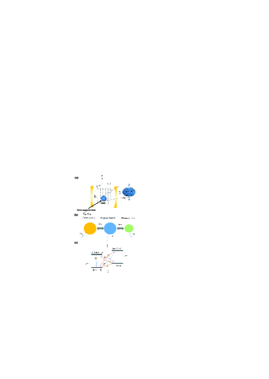
Figure 1: (a) Schematic illustration of the system, a YIG sphere is placed in the maximum magnetic field of a microwave cavity mode. And an uniform external bias magnetic field H is applied along the z-direction to bias the YIG sphere. The enlarged YIG sphere on the right illustrates how the dynamic magnetization of magnon (vertical black arrows) causes the deformation (compression along the y-direction) of the YIG sphere (and vice versa), which rotates at the magnon frequency. Furthermore, a microwave source is used to drive the magnon mode. It’s important to note that the bias magnetic field (z direction), the drive magnetic field (y direction), and the magnetic field (x direction) of the cavity mode are mutually perpendicular at the site of the YIG sphere. (b) The equivalent coupled-harmonic-resonator model. (c) Energy levels diagram of the effective Hamiltonian in Eq.(10), $\left|m,n\right\rangle$ denotes the number state with $m$ the magnon number of the magnon mode and $n$ the phonon number of the mechanical mode.

The quantum Langevin equations of the linearized Hamiltonian $H_{lin}$ in Eq.(II) are given by

$$\dot{a} = (i\Delta_{a}-\kappa_{a})a-ig_{ma}^{\ast}m-\sqrt{2\kappa_{a}}a_{in},$$

$$\dot{m} = (i\Delta_{m}-\kappa_{m})m-ig_{ma}a-iG(b+b^{\dagger})$$

$$-\sqrt{2\kappa_{m}}m_{in},$$

$$\dot{b} = (-i\omega_{b}-\gamma_{b})b-i(G^{\ast}m+Gm^{\dagger})-\sqrt{2\gamma_{b}}b_{in},$$

where $a_{in},m_{in}$ and $b_{in}$ are the corresponding noise operators, the correlation functions can be found in the appendix A. To make the following result within experimental realizations, the parameters are in accord with recent cavity magnomechanical work k1 ; k0 ; k151 , i.e., $\omega_{a}/2\pi=$ $\omega_{m}/2\pi=10.1GHz$ of the Kittle mode, $\gamma_{b}/2\pi=100Hz,\kappa_{a}/2\pi=1GHz,\kappa_{m}/2\pi=0.15MHz,\omega_{b}/2\pi=10MHz$, the coupling strength $g_{ma}/2\pi=20MHz$ and $g_{mb}/2\pi=$ $0.1Hz$. Here, our research is in resolved sideband regime ($\kappa_{m}/\omega_{b}<1$).

For this system, cavity mode $a$ does not directly interact with the mechanical mode $b$. In order to study the influence of magnon mode on cooling of the mechanical resonator and make our calculations more convenient, we show a effective Hamiltonian by assuming the mode $a$ is highly dissipative. In the limit that $\kappa_{a}\gg g_{ma},G,\kappa_{m}$, we can adiabatically eliminate mode $a$ g1 . The equation about $a$ in Eq.(II) can be solved.

$$a=\frac{ig_{ma}^{\ast}m+\sqrt{2\kappa_{a}}a_{in}}{i\Delta_{a}-\kappa_{a}}.$$ (5)

Then we insert Eq.(5) into the term of $m$ in Eq.(II), the effective Langevin equation for $m$ is given by

$$\dot{m}=(i\Delta_{eff}-\kappa_{eff})m-iG(b+b^{\dagger})-m_{eff,in},$$ (6)

where the effective parameters can be written as

$$\Delta_{eff}=\Delta_{m}-\frac{\left|g_{ma}\right|^{2}}{\Delta_{a}^{2}+\kappa_{a}^{2}}\Delta_{a},$$ (7)

$$\kappa_{eff}=\kappa_{m}+\frac{\left|g_{ma}\right|^{2}}{\Delta_{a}^{2}+\kappa_{a}^{2}}\kappa_{a},$$ (8)

$$m_{eff,in}=\frac{ig_{ma}\sqrt{2\kappa_{a}}a_{in}}{i\Delta_{a}-\kappa_{a}}-\sqrt{2\kappa_{m}}m_{in},$$ (9)

where $\Delta_{eff}$ is the effective detuning between input drive magnetic field and magnetic resonance, $\kappa_{eff}$ is the effective decay rate of the magnon mode and $m_{eff,in}$ is the effective noise operator of the magnon mode. Note that the effective coupling strength is still $G.$

After adiabatically eliminating optical mode $a$ and using the effective parameters we got before, the effective Hamiltonian reads

$$H_{eff}=-\Delta_{eff}m^{\dagger}m+\omega_{b}b^{\dagger}b+(Gm^{\dagger}+G^{\ast}m)(b+b^{\dagger}).$$ (10)

This effective Hamiltonian make the system transform from the three-level system to an effective two-level system. The above $H_{eff}$ can also be obtained by the method of effective master equation g8 .

In Fig. 1(c), we show the level diagram of the linearized Hamiltonian in Eq.(10). There are three kinds of heating processes corresponding to A, B and C. A represents the swap heating, B represents the quantum backaction heating and C represents thermal heating, C is an incoherent process arising from the interaction between the mechanical object and the environment. Our ultimate goal is to suppress thermal heating, the swap heating and quantum backaction heating are the accompanying effect, corresponding to the coherent interaction processes $mb^{\dagger}$ and $m^{\dagger}b^{\dagger}$, respectively. The swap heating originates from the energy exchange between the magnon mode and the phonon mode, it emerges when the system is in the strong magnomechanical coupling regime. Meanwhile, quantum backaction heating can lead to a fundamental limit for backaction cooling. The cooling processes D, E, and F are related to the energy swapping, counter-rotating-wave interaction between the magnon mode and the phonon mode, and the dissipation of magnon mode.

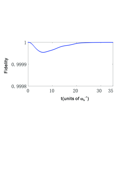
Figure 2: The numerical result of fidelity between the exact state $\rho$ and the effective state $\rho_{eff}$ as a function of $t(\omega_{b}^{-1}).$ The parameters we chosen are the same as those in Fig. 3.

In order to better prove the accuracy of $H_{eff}$ obtained, we show the fidelity between the exact state $\rho$ and the effective state $\rho_{eff}$ as a function of $t(\omega_{b}^{-1})$ in Fig. 2, where $\rho$ and $\rho_{eff}$ are the numerical results of $H_{lin}$ in Eq.(II) and $H_{eff}$ in Eq.(10) calculated by quantum master equation $\dot{\rho}=i[\rho,H]+\kappa_{a}\mathcal{D}[a]\rho+\kappa_{m}\mathcal{D}[m]\rho+\gamma_{b}(n_{th}+1)\mathcal{D}[b]\rho+\gamma_{b}n_{th}\mathcal{D}[b^{\dagger}]\rho$, where $\mathcal{D}[o]\rho=o\rho o^{\dagger}-o^{\dagger}o\rho/2-\rho o^{\dagger}o/2$ $(o=a,m,b)$ are Lindblad superoperators of our system. Here we choose the same initial state, so fidelity evolved from 1, then it decreases slightly over time and reaches $1$ finally. The reason for slight decrease is the cavity mode $a$ is highly dissipative. Fig. 2 implies that our effective Hamiltonian $H_{eff}$ is valid and a good approximation.

III Magnomechanical Cooling

We analyze the ground-state cooling of the whole system in the cases of weak and strong magnomechanical coupling. In the weak magnomechanical coupling regime, similar to dealing with such problems in optomechanical systems, we use quantum noise approach to get the extra magnetic damping $\Gamma_{{}_{md}}$ for the magnomechanical resonator (see Appendix B)

$$\Gamma_{md} = -2\text{Im}\Sigma(\omega_{b})$$

$$= 2\left|G\right|^{2}\text{Re}[\frac{1}{-i(\omega_{b}+\Delta_{eff})+\kappa_{eff}}$$

$$-\frac{1}{-i(\omega_{b}-\Delta_{eff})+\kappa_{eff}}].$$

By solving the rate equation in the steady state, the final phonon number can be analytically described by

$$n_{f}=\frac{A_{+}+\gamma_{b}n_{th}}{\Gamma_{{}_{md}}+\gamma_{b}},$$ (12)

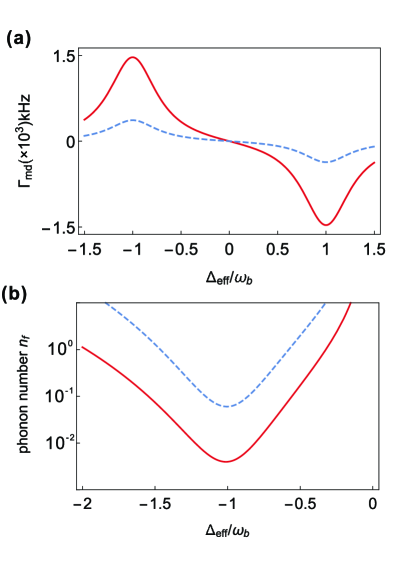
Figure 3: (a) damping $\Gamma_{{}_{md}}$ versus $\Delta_{eff}$ with two coupling strengths $G/\omega_{b}=0.15$ (red solid curve) and $0.075$ (blue dotted curve). (b) the final phonon number $n_{f}$ versus $\Delta_{eff}$ with two coupling strengths $G/\omega_{b}=0.15$ (red solid curve) and $0.075$ (blue dotted curve). Here we set $\omega_{b}/2\pi=10MHz$, $\gamma_{b}/\omega_{b}=10^{-5},n_{th}=1000,\kappa_{eff}/\omega_{b}\simeq 0.3$, $\kappa_{m}/\omega_{b}=0.15,\kappa_{a}/\omega_{b}=1\times 10^{2},$ $g_{ma}/\omega_{b}=2$ and $\Delta_{a}/\omega_{b}=1.$

where $A_{+}$ is the heating rate, its detailed expressions can be found in Appendix B. $n_{th}=(e^{\hbar\omega_{b}/k_{B}T}-1)$ is thermal phonon number of the mechanical resonator, $T$ is the environmental temperature and $k_{B}$ is the Boltzmann constant. Here, $n_{f}$ can also be regarded as the cooling limit. And it can be divided into two parts, one part is the classical cooling limit $\gamma_{b}n_{th}/(\Gamma_{{}_{md}}+\gamma_{b})$, the other part is the quantum cooling part $A_{+}/(\Gamma_{{}_{md}}+\gamma_{b})$ and it corresponds to the heating rate $A_{+}$ originates from the quantum backaction.

Fig. 3(a) shows the extra magnetic damping $\Gamma_{{}_{md}}$ under different $\Delta_{eff}/\omega_{b}$ with two coupling strengths $G/\omega_{b}=0.15$ and $G/\omega_{b}=0.075$, respectively. It can be seen that the maximum magnetic damping (gain) is located at the point $\Delta_{eff}=-\omega_{b}(\omega_{b}).$ From Eq.(III) and Eq.(12), $n_{f}$ decreases with the increase of $\Gamma_{{}_{md}}$. Fig. 3(b) shows the final phonon number $n_{f}$ under different $\Delta_{eff}/\omega_{b}$ with two coupling strengths, respectively. It shows the minimum $n_{f}$ is located at the detuning point $\Delta_{eff}=-\omega_{b}.$When $G/\omega_{b}=0.15$ and $G/\omega_{b}=0.075$, the minimums of $n_{f}$ are about $10^{-2}$ and $10^{-1}$ respectively, ground-state cooling of the magnomechanical resonator can be achieved. Moreover, compared to the two different $G$ in Fig. 3(a) and Fig. 3(b), it can be known that the stronger $G$, the better effect of ground-state cooling in weak coupling regime ($G<$ $\kappa_{eff}$).

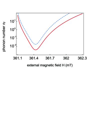
Figure 4: The final phonon number $n_{f}$ versus the external magnetic field $H$ with two coupling strengths $G/\omega_{b}=0.15$ (red solid curve) and $0.1$ (blue dotted curve). The other parameters are the same as those in Fig. 3.

In order to study the influence of magnon mode on the cooling of the oscillator, in Fig. 4, we plot the final phonon number $n_{f}$ under different external magnetic field $H$ with two coupling strengths. We find that for external magnetic field $H$, there is an obvious window in which the ground-state cooling can appear. It shows the ground-state cooling of the mechanical resonator can be controlled by tuning $H$, which presents an additional degree of freedom in cavity optomechanical systems. By comparing two different coupling strengths $G$, increasing coupling strength widens the window for ground-state cooling. Note that the external magnetic field $H$, the drive magnetic field and the magnetic field of the cavity mode are mutually perpendicular at the site of the YIG sphere. Consequently, we can just tune $H$ without affecting the other two.

The recent work shows the strong coupling between magnon mode $m$ and mechanical mode $b$ can be achieved. From Eq.(10), the covariance approach is used to calculate the mean phonon number $N_{bs}$ in steady state (see Appendix C), and this approach is applicable to both cases of strong couling and weak coupling.

$$N_{bs} \simeq \frac{4\left|G\right|^{2}+\kappa_{eff}^{2}}{4\left|G\right|^{2}(\gamma_{b}+\kappa_{eff})}\gamma_{b}n_{th}$$

$$+\frac{4\omega_{b}^{2}(\kappa_{eff}^{2}+8\left|G\right|^{2})+\kappa_{eff}^{2}(\kappa_{eff}^{2}-8\left|G\right|^{2})}{16\omega_{b}^{2}(4\omega_{b}^{2}+\kappa_{eff}^{2}-16\left|G\right|^{2})}.$$

For $G/\omega_{b}=0.4$ $(G>\kappa_{eff}),$ the other parameters are the same as those in Fig. 3, we have $N_{bs}\simeq 0.257$ by Eq.(III). Under the same parameters, the numerical solution of the mean phonon number obtained from the quantum master equation is shown in Fig. 5. Here, we only need to numerically calculate the mean values of all the second-order moments instead of the matrix elements of the density operator $\rho$ (see Appendix C). The cut-off of the density matrix is not necessary and the solutions are exact. It can be seen that the numerical solution $N_{bs}$ tends to be stable at $0.28$ after a period of oscillation. This agrees roughly with the analytical result. Note that the analytical and numerical solution are both obtained under condition $\Delta_{eff}=-$ $\omega_{b}.$The results show that ground-state cooling can be achieved in strong coupling regime.

The dynamical stability condition of our system can be given by the Routh-Hurwitz criterion g7 . Y. C. Liu, $et$ $al$ discussed a similar two-mode coupled system g6 . Referring to their results, the steady-state condition here is $\left|G\right|^{2}<\omega_{b}^{2}/4+\kappa_{eff}^{2}/16$ with the detuning $\Delta_{eff}=-\omega_{b}$. And the parameters used here are all satisfied with the stability condition.

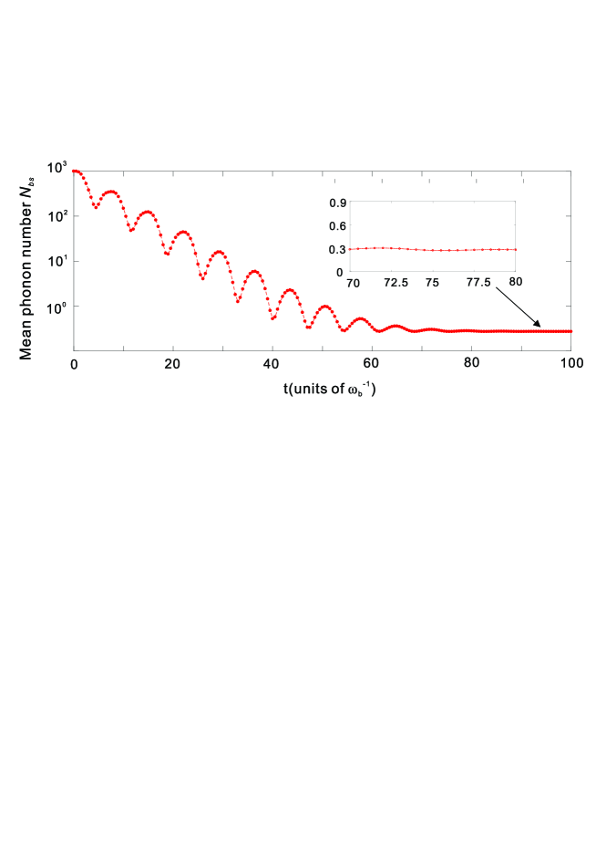
Figure 5: The numerical result of the mean phonon number $N_{bs}$ as a function of $t(\omega_{b}^{-1}).$ Here, we set $G/\omega_{b}=0.15$, the other parameters are the same as those in Fig. 3.

Our discussion is on the premise of low-lying excitation, which is $\left\langle m^{\dagger}m\right\rangle$ $\ll 2Ns=5N$ ($N$ is the total number of spins). For a 1-$mm$-diam YIG sphere k2 ; k6 , $N=$ $\Lambda V\approx 2.2\times 10^{18}$, where $\Lambda=4.22\times 10^{27}$ is the spin density of the YIG and $V$ is the volume of the sphere. For $G/2\pi=4MHz$, we have $\left|\eta\right|=4\times 10^{7}$. Finally $\left\langle m^{\dagger}m\right\rangle=1.6\times 10^{15}\ll 5N\approx$ $1.1\times 10^{19}$, the condition of low-lying excitation is satisfied.

The strong magnon drive we used will led to the unwanted Kerr nonlinear term $\mathcal{K}m^{\dagger}mm^{\dagger}m$ in the Hamiltonian, where $\mathcal{K}$ is the Kerr coefficient. For the 1-$mm$-diam YIG sphere, $\mathcal{K}/2\pi\approx 10^{-10}Hz$. For $G/2\pi=4MHz$, we have $\varepsilon_{d}=4\times 10^{14}Hz.$ When the parameters satisfie the condition $\mathcal{K}\left|\left\langle m\right\rangle\right|^{3}\ll\varepsilon_{d}$, Kerr nonlinear term can be neglected. Here, $\mathcal{K}\left|\left\langle m\right\rangle\right|^{3}=6.4\times 10^{12}\ll\varepsilon_{d}=4\times 10^{14}Hz$. Therefore, it implies that our linearized model is a good approximation.

IV Conclusions

In summary, we have studied ground-state cooling in a cavity magnomechanical system, which has three modes: cavity photon mode, magnon mode and phonon mode. The magnon and mechanical modes are coupled to each other through the magnetostrictive interaction. By assuming the cavity mode is highly dissipative, we adiabatically eliminate cavity mode, and the effective Hamiltonian is given. Which is consist of two mode: magnon mode and phonon mode. Then we study the final phonon number numerically and analytically. And we find the ground-state cooling of magnomechanical resonator can be achieved by using experimentally feasible parameters. Different from the existing optomechanical cooling system, the extra magnetic damping is the reason of cavity magnomechanical cooling intrinsically. In other words, we can utilize magnon mode to achieve the cooling of mechanical mode. Furthermore, the ground-state cooling can be well controlled by adjusting the magnetic field without changing other parameters, which provides an additional degree of freedom.

Because the cavity magnomechanical system has intrinsic great tunability, low loss, and promising integration with electromechanical elements, we believe that the proposed scheme provides a promising platform to the further investigation of cooling of mechanical resonator. And we hope it opens up new way to the foundations of quantum physics and applications. In addition, cooling the mechanical system to its quantum ground state is also an important guarantee for realizing quantum operations in quantum information processing.

Appendix A linearization of Hamiltonian

From Eq.(II), the quantum Langevin equations (QLEs) of the system are given by

$$\dot{a} = (i\Delta_{a}-\kappa_{a})a-ig_{ma}m-\sqrt{2\kappa_{a}}a_{in},$$

$$\dot{m} = (i\Delta_{m}-\kappa_{m})m-ig_{ma}a-ig_{mb}m(b+b^{\dagger})$$

$$+\varepsilon_{d}-\sqrt{2\kappa_{m}}m_{in},$$

$$\dot{b} = (-i\omega_{b}-\gamma_{b})b-ig_{mb}m^{\dagger}m-\sqrt{2\gamma_{b}}b_{in},$$

where $$a_{in},m_{in} b_{in}$$ and are the corresponding noise operators with zero mean values, and the correlation functions for these noise operators can be written as

$$\left\langle a_{in}(t)a_{in}^{\dagger}(t^{\prime})\right\rangle = \delta(t-t^{\prime}),$$

$$\left\langle a_{in}^{\dagger}(t)a_{in}(t^{\prime})\right\rangle = 0,$$

$$\left\langle m_{in}(t)m_{in}^{\dagger}(t^{\prime})\right\rangle = \delta(t-t^{\prime}),$$ (15a)

$$\left\langle m_{in}^{\dagger}(t)m_{in}(t^{\prime})\right\rangle = 0,$$

$$\left\langle b_{in}(t)b_{in}^{\dagger}(t^{\prime})\right\rangle = (n_{th}+1)\delta(t-t^{\prime}),$$

$$\left\langle b_{in}^{\dagger}(t)b_{in}(t^{\prime})\right\rangle = n_{th}\delta(t-t^{\prime}),$$

where $$n_{th} n_{th}=(e^{\hbar\omega_{b}/k_{B}T}-1) T k_{B}$$ is thermal phonon number of the mechanical resonator, and it can be regarded as , is the environmental temperature and is the Boltzmann constant.

Then we rewrite each Heisenberg operator as a sum of its steady-state mean value and the quantum fluctuations, i.e., $a=\alpha+a,m=\eta+m$ and $b=\beta+b.$ By separating the classical and quantum components, the quantum Langevin equations (QLEs) can be rewritten as

$$\dot{a} = (i\Delta_{a}-\kappa_{a})a-ig_{ma}^{\ast}m-\sqrt{2\kappa_{a}}a_{in},$$

$$\dot{m} = (i\tilde{\Delta}_{m}-\kappa_{m})m-ig_{mb}\eta(b+b^{\dagger})$$

$$-ig_{mb}m(b+b^{\dagger})-ig_{ma}a-\sqrt{2\kappa_{m}}m_{in},$$

$$\dot{b} = (-i\omega_{b}-\gamma_{b})b-ig_{mb}(\eta^{\ast}m+\eta m^{\dagger})-ig_{mb}m^{\dagger}m$$

$$-\sqrt{2\gamma_{b}}b_{in},$$

where $$\tilde{\Delta}_{m}=\Delta_{m}-g_{mb}(\beta+\beta^{\ast}) ig_{mb}m(b+b^{\dagger}) ig_{mb}m^{\dagger}m$$. Here, under the strong driving condition, the nonlinear terms and can be neglected, then we have linearized quantum Langevin equations, and the Hamiltonian in Eq.(II) is rewritten as an linearized Hamiltonian

$$H_{lin} = -\Delta_{a}a^{\dagger}a-\tilde{\Delta}_{m}m^{\dagger}m+\omega_{b}b^{\dagger}b$$ (17a)

$$+(Gm^{\dagger}+G^{\ast}m)(b+b^{\dagger})$$

$$+(g_{ma}m^{\dagger}a+g_{ma}^{\ast}ma^{\dagger}),$$

where $$G=\eta g_{mb} \tilde{\Delta}_{m}=\Delta_{m}-g_{mb}(\beta+\beta^{\ast})$$ is the coherent-driving-enhanced magnomechanical coupling strength, and is the modified detuning of the magnon mode.

Appendix B weak coupling

Similar to the method used in cavity optomechanical systems, we study the cooling rate of the magnomechanical resonator by using the quantum noise spectrum of the magnetic force.

In weak coupling regime ($G<$ $\kappa_{eff}$), the quantum noise approach is feasible. From Eq.(10), $F_{m}(t)=\tilde{m}\ddot{x}+\tilde{m}\omega_{b}^{2}x$ and $\dot{p}+\tilde{m}\omega_{b}^{2}x=-\frac{1}{x_{ZPF}}[G^{\ast}m(t)+Gm^{\dagger}(t)]$, the magnetic force operator can be obtained as

$$F_{m}(t)=-\frac{1}{x_{ZPF}}[G^{\ast}m(t)+Gm^{\dagger}(t)],$$ (18a)

where $$\tilde{m} p x=x_{ZPF}(b+b^{\dagger}) x_{ZPF}=\sqrt{1/(2\tilde{m}\omega_{b})} x_{ZPF}$$ is the effective mass of the mechanical resonator, is the momentum operator, is the position operator and ( is the zero-point fluctuation amplitude of the mechanical oscillator). Using the Fourier transform of the autocorrelation functions, the quantum noise spectrum is given by

$$S_{FF}(\omega)=\int\left\langle F_{m}(t)F_{m}(0)\right\rangle e^{i\omega t}dt.$$ (19a)

In the absence of the magnomechanical coupling, the term of $m$ in the Langevin equations of the effective Hamiltonian $H_{eff}$ can be expressed as

$$-i\omega m(\omega) = (i\Delta_{eff}-\kappa_{eff})m(\omega)$$ (20a)

$$-\sqrt{2\kappa_{eff}}m_{eff,in}.$$

Here, we transform $m(t)$ to the frequency domain. Then using Eq.(18a) and Eq.(19a), the spectral density of the magnetic force is described by

$$S_{FF}(\omega)=\frac{2\kappa_{eff}\left|G\chi(\omega)\right|^{2}}{x_{ZPF}^{2}},$$ (21)

where the response function is

$$\chi(\omega)=\frac{1}{-i(\omega+\Delta_{eff})+\kappa_{eff}}.$$ (22a)

The cooling and heating rates can be given by $A_{-}=S_{FF}(\omega)x_{ZPF}^{2}$ and $A_{+}=S_{FF}(-\omega)x_{ZPF}^{2}$, respectively. And they correspond to the rates for absorbing and emitting a phonon, respectively.

By considering the magnomechanical coupling, the Langevin equations of the effective Hamiltonian $H_{eff}$ are given by

$$-i\omega m(\omega) = (i\Delta_{eff}-\kappa_{eff})m(\omega)$$ (23a)

$$-iG[b(\omega)+b^{\dagger}(\omega)]$$

$$-\sqrt{2\kappa_{eff}}m_{eff,in}(\omega),$$

$$-i\omega b(\omega) = (-i\omega_{b}-\gamma_{b})b(\omega)$$ (23b)

$$-i[G^{\ast}m(\omega)+G(\omega)m^{\dagger}(\omega)]$$

$$-\sqrt{2\gamma_{b}}b_{in}(\omega),$$

where noise operators $$m_{eff,in}(\omega) b_{in}(\omega)$$ and are the corresponding noise operators in the frequency domain. from which we obtain

$$b(\omega)\simeq\frac{\sqrt{2\gamma_{b}}b_{in}(\omega)-i\sqrt{2\kappa_{eff}}f(\omega)}{i\omega-i[\omega_{b}+\Sigma(\omega)]-\gamma_{b}},$$ (24)

where $$f(\omega)=G^{\ast}\chi(\omega)m_{eff,in}(\omega)+G\chi^{\ast}(-\omega)m_{eff,in}^{\dagger}(\omega) \omega\simeq\omega_{b} b^{\dagger}(\omega) \Sigma(\omega)=-i\left|G\right|^{2}[\chi(\omega)-\chi^{\ast}(-\omega)] \delta\omega_{b} \Gamma_{{}_{md}}$$. The reason for the approximation is we consider , in this way, the terms containing can be neglected. is the magnomechanical self energy. Then the frequency shift and the extra magnetic damping are given as

$$\delta\omega_{b} = \text{Re}\Sigma(\omega),$$ (25a)

$$\Gamma_{{}_{md}} = -2\text{Im}\Sigma(\omega)=A_{-}-A_{+}.$$ (25b)

Using similar methods in cavity optomechanical systems, from the rate equation for the probability $P_{n}(t)$ and the average phonon number $\bar{n}=\sum_{n=0}^{\infty}nP_{n}$ k00 , and after making

$\dot{\bar{n}}=0$, we have the final phonon number $n_{f}$

$$n_{f}=\frac{A_{+}+\gamma_{b}n_{th}}{\Gamma_{{}_{md}}+\gamma_{b}}.$$ (26a)

Appendix C Strong coupling

Because of the introduction of external drive magnetic field, the whole system can enable strong coupling ($G>$ $\kappa_{eff}$) between magnon mode $m$ and mechanical mode $b$ by adjusting the intensity of driving field.

For the linear regime under strong driving, the mean phonon number can be computed exactly by the quantum master equation. From the effective Hamiltonian in Eq.(10), the quantum master equation can be described by

$$\dot{\rho} = i[\rho,H_{eff}]m+\kappa_{eff}\mathcal{L(}m)\rho$$ (27a)

$$+\gamma_{b}(n_{th}+1)\mathcal{L(}b)\rho$$

$$+\gamma_{b}n_{th}\mathcal{L(}b^{\dagger})\rho,$$

where the Lindblad superoperators are given by

$$\mathcal{L(}o)\rho=o\rho o^{\dagger}-o^{\dagger}o\rho/2-\rho o^{\dagger}o/2(o=m,b).$$ (28a)

Since the Hamiltonian is linear, we can only calculate the mean values of all the second-order moments, Such as $\left\langle m^{\dagger}m\right\rangle,\left\langle b^{\dagger}b\right\rangle,\left\langle m^{\dagger}b\right\rangle,\left\langle mb\right\rangle,\left\langle m^{2}\right\rangle,\left\langle b^{2}\right\rangle$ and the conjugation of the last four terms. In the stable regime, under the conditions $\Delta_{eff}=-$ $\omega_{b}$ and $4\left|G\right|^{2}/(\gamma_{b}\kappa_{eff})\gg 1$, $N_{bs}$ is calculated as

$$N_{bs} \simeq \frac{4\left|G\right|^{2}+\kappa_{eff}^{2}}{4\left|G\right|^{2}(\gamma_{b}+\kappa_{eff})}\gamma_{b}n_{th}$$

$$+\frac{4\omega_{b}^{2}(\kappa_{eff}^{2}+8\left|G\right|^{2})+\kappa_{eff}^{2}(\kappa_{eff}^{2}-8\left|G\right|^{2})}{16\omega_{b}^{2}(4\omega_{b}^{2}+\kappa_{eff}^{2}-16\left|G\right|^{2})}.$$

Note that no cut-off of the density matrix is required in this solution, and it holds for both weak and strong coupling regimes.

References

- (1) G. Khitrova, H. M. Gibbs, M. Kira, S.W. Koch, and A. Scherer, Nat. Phys. 2, 81 (2006).
- (2) S. B. Zheng and G. C. Guo, Phys. Rev. Lett. 85, 2392 (2000).
- (3) J. I. Cirac, P. Zoller, H. J. Kimble, and H. Mabuchi,Phys. Rev. Lett. 78, 3221 (1997).
- (4) C. Monroe, D. M. Meekhof, B. E. King, S. R. Jefferts, W. M. Itano, D. J. Wineland, and P. Gould, Phys. Rev. Lett. 75, 4011 (1995).
- (5) P. Pei, F. Y. Zhang, C. Li, and H. S. Song, Phys. Rev. A 84, 042339 (2011).
- (6) O. Soykal, and M. E. Flatté, Phys. Rev. Lett. 104, 077202 (2010).
- (7) O. Soykal and M. E. Flatté Size dependence of strong coupling between nanomagnets and photonic cavities, Phys. Rev. B 82, 104413 (2010).
- (8) X. F. Zhang, C. L. Zou, L. Jiang, and H. X. Tang, Phys. Rev. Lett. 113, 156401 (2014).
- (9) S. Sharma, Y. M. Blanter, and G. E. W. Bauer, Optical Cooling of Magnons, Phys. Rev. Lett. 121, 087205 (2018).
- (10) A. Osada, A. Gloppe, R. Hisatomi, A. Noguchi, R. Yamazaki, M. Nomura, Y. Nakamura, and K. Usami, Brillouin Light Scattering by Magnetic Quasivortices in Cavity Optomagnonics, Phys. Rev. Lett. 120, 133602 (2018).
- (11) A. Osada, R. Hisatomi, A. Noguchi, Y. Tabuchi, R. Yamazaki, K. Usami, M. Sadgrove, R. Yalla, M. Nomura, and Y. Nakamura, Cavity Optomagnonics with Spin-Orbit Coupled Photons, Phys. Rev. Lett. 116, 223601 (2016).
- (12) J. A. Haigh, A. Nunnenkamp, A. J. Ramsay, and A. J. Ferguson, Triple-Resonant Brillouin Light Scattering in Magneto-Optical Cavities, Phys. Rev. Lett. 117, 133602 (2016).
- (13) N. Kostylev, M. Goryachev, and M. E. Tobar, Superstrong Coupling of a Microwave Cavity to Yttrium iron Garnet Magnons, Appl. Phys. Lett. 108, 062402 (2016).
- (14) C. Kittel, Phys. Rev. 73, 155 (1948).
- (15) H. Huebl, C. W. Zollitsch, J. Lotze, F. Hocke, M. Greifenstein, A. Marx, R. Gross, and S. T. B. Goennenwein, High Cooperativity in Coupled Microwave Resonator Ferrimagnetic Insulator Hybrids, Phys. Rev. Lett. 111, 127003 (2013).
- (16) Y. Tabuchi, S. Ishino, T. Ishikawa, R. Yamazaki, K. Usami, and Y. Nakamura, Hybridizing Ferromagnetic Magnons and Microwave Photons in the Quantum Limit, Phys. Rev. Lett. 113, 083603 (2014).
- (17) J. Bourhill, N. Kostylev, M. Goryachev, D. L. Creedon, and M. E. Tobar, Ultrahigh cooperativity interactions between magnons and resonant photons in a YIG sphere, Phys. Rev. B 93, 144420 (2016).
- (18) Y. P. Wang, G. Q. Zhang, D. Zhang, T. F. Li, C. M. Hu, and J. Q. You, ”Bistability of Cavity Magnon Polaritons,” Phys. Rev. Lett. 120, 057202 (2018).
- (19) G. Q. Zhang and J. Q. You, Phys. Rev. B 99, 054404 (2019).
-
(20)
Y. P. Wang, G. Q. Zhang, D. Zhang, X. Q. Luo, W. Xiong, S. P.
Wang, T. F. Li, C. M. Hu, and J. Q. You, ”Magnon Kerr effect in a strongly
coupled cavity-magnon system,” Phys. Rev. B 94, 224410 (2016).
- (21) B. Wang, Z. X. Liu, C. Kong, H. Xiong, and Y. Wu, ”Magnon-induced transparency and amplification in PT symmetric cavity-magnon system,” Opt. Express 26, 20248-20257 (2018).
- (22) M. Goryachev, S. Watt, J. Bourhill, M. Kostylev, and M. E. Tobar, Phys. Rev. B 97, 155129 (2018).
- (23) B. Wang, C. Kong, Z. X. Liu, H. Xiong, and Y. Wu, Laser. Phys. Lett. 16, 045208 (2019).
- (24) L. Bai, M. Harder, Y. P. Chen, X. Fan, J. Q. Xiao, and C.-M. Hu, ”Spin Pumping in Electrodynamically Coupled Magnon-Photon Systems,” Phys. Rev. Lett. 114, 227201 (2015).
- (25) M. Goryachev, W. G. Farr, D. L. Creedon, Y. Fan, and M. E. Tobar, ”High-cooperativity cavity QED with magnons at microwave frequencies,” Phys. Rev. Applied. 2, 054002 (2014).
- (26) Z. X. Liu, B. Wang, H. Xiong, and Y. Wu, ”Magnon-induced high-order sideband generation,” Opt. Lett. 43, 3698 (2018).
- (27) M. Aspelmeyer, T. J. Kippenberg, and F. Marquardt, Rev. Mod. Phys. 86, 1391 (2014).
- (28) M. Li, W. Pernice, C. Xiong, J. T. Baehr, M. Hochberg, and H. X. Tang, Nature 456, 480 (2008).
- (29) M. Aspelmeyer, P. Meystre, and K. Schwab, Phys. Today 65, 29 (2012).
- (30) A. H. Safavi-Naeini, T. P. Mayer Alegre, J. Chan, M. Eichenfield, and O. Painter, Nature 472, 69 (2011).
- (31) B. Xiong, Li. X, S. L. Chao, and L. Zhou, Opt. Lett. 43, 6053–6056 (2018).
- (32) P. Rabl, “Photon blockade effect in optomechanical systems,” Phys. Rev. Lett. 107, 063601 (2011).
- (33) G. Heinrich, M. Ludwig, J. Qian, B. Kubala, and F. Marquardt, Phys. Rev. Lett. 107, 043603 (2011).
- (34) T. P. Purdy, P. L. Yu, R. W. Peterson, N. S. Kampel, and C. A. Regal, Phys. Rev. X. 3, 031012 (2013).
- (35) J. Q. Liao and F. Nori, Phys. Rev. A 88, 023853 (2013).
- (36) J. Li, S. Y. Zhu, and G. S. Agarwal, ”Magnon-photon-phonon entanglement in cavity magnomechanics”. Phys. Rev. Lett. 121, 203601 (2018).
- (37) X. Zhang, C. L. Zou, L. Jiang, and H. X. Tang, ”Cavity magnomechanics,” Sci. Adv. 2, e1501286 (2016).
- (38) J. Li, S. Y. Zhu, and G. S. Agarwal, ”Squeezed states of magnons and phonons in cavity magnomechanics,” Phys. Rev. A 99, 021801 (2019).
- (39) S. N. Huai, Y. L. Liu, J. Zhang, L. Yang, and Y. X. Liu, Phys. Rev. A 99, 043803 (2019).
- (40) Y. P. Gao, C. Cao, T. J. Wang, Y. Zhang, and C. Wang, ”Cavity-mediated coupling of phonons and magnons,” Phys. Rev. A 96, 023826 (2017).
- (41) Y. L. Liu and Y. X. Liu, Phys. Rev. A 96, 023812 (2017).
- (42) Y. C. Liu, X. Y. Xiao, X. S. Luan, Q. H. Gong, and C. W. Wong, Phys. Rev. A 91, 033818 (2015).
- (43) F. Marquardt, J. P. Chen, A. A. Clerk, and S. M. Girvin, Quantum Theory of Cavity-Assisted Sideband Cooling of Mechanical Motion, Phys. Rev. Lett. 99, 093902 (2007).
- (44) I. Wilson-Rae, N. Nooshi, W. Zwerger, and T. J. Kippenberg, Theory of Ground State Cooling of a Mechanical Oscillator Using Dynamical Backaction, Phys. Rev. Lett. 99, 093901 (2007).
- (45) I. Wilson-Rae, N. Nooshi, J. Dobrindt, T. J. Kippenberg, and W. Zwerger, Cavity-assisted backaction cooling of mechanical resonators, New J. Phys. 10, 095007 (2008).
- (46) S. Grölacher, J. B. Hertzberg, M. R. Vanner, S. Gigan, K. C. Schwab, and M. Aspelmeyer, Demonstration of an ultracold microoptomechanical oscillator in a cryogenic cavity, Nat. Phys. 5, 485 (2009).
- (47) Y. S. Park and H. Wang, Resolved-sideband and cryogenic cooling of an optomechanical resonator, Nat. Phys. 5, 489 (2009).
- (48) Meenehan S M, Cohen J D, MacCabe G S, et al. Pulsed excitation dynamics of an optomechanical crystal resonator near its quantum ground state of motion[J]. Physical Review X, 2015, 5(4): 041002.
- (49) Zhou B, Li G. Ground-state cooling of a nanomechanical resonator via single-polariton optomechanics in a coupled quantum-dot–cavity system[J]. Physical Review A, 2016, 94(3): 033809.
- (50) Fogarty T, Landa H, Cormick C, et al. Optomechanical many-body cooling to the ground state using frustration[J]. Physical Review A, 2016, 94(2): 023844.
- (51) Z. Q. Yin, W. L. Yang, L. Y. Sun, and L. M. Duan, Phys. Rev. A 91, 012333 (2015).
- (52) Y. C. Liu, Y. F. Xiao, X. S. Luan, and C. W. Wong, Phys. Rev. Lett. 110, 153606 (2013).
- (53) Y. C. Liu, W. H. Yu, C. W. Wong, and Y. F. Xiao, Chin. Phys. B 22, 114213 (2013).
- (54) E. X. DeJesus and C. Kaufman, Routh-Hurwitz criterion in then examination of eigenvalues of a system of nonlinear ordinary differential equations, Phys. Rev. A 35, 5288 (1987).
- (55) Y. X. Zeng, J. Shen, T. Gebremariam, and C. Li, Quantum. Inf. Process 18, 205 (2019).
- (56) Y. X. Zeng, T. Gebremariam, M. S. Ding, and C. Li, J. Opt. Soc. Am. B 35, 2334 (2018).