Dynamical $t/U$ Expansion of blackthe Doped Hubbard Model

Abstract

blackWe construct a new $U(1)$ slave spin representation for the single band Hubbard model in the large-$U$ limit. blackThe mean-field theory in this representation is more amenable to describe blackboth the spin-charge-separation physics of the Mott insulator at half-filling blackand the strange metal behavior at finite doping. By employing a dynamical Green’s function theory blackfor slave spins, we calculate the single-particle spectral function of electrons, and the result is comparable to blackthat in dynamical mean field theories. blackWe then formulate a dynamical $t/U$ expansion for the blackdoped Hubbard model blackthat reproduces the mean-field results at the lowest order of expansion. To the next order of expansion, it naturally yields an effective low-energy theory of a $t-J$ model for spinons self-consistently coupled to an $XXZ$ model for the slave spins. blackWe show that the superexchange $J$ is renormalized by doping, in agreement with the Gutzwiller approximation. blackSurprisingly, we find a new ferromagnetic channel blackof exchange interactions which blacksurvives in the infinite $U$ limit, as a manifestation of the Nagaoka ferromagnetism.

Introduction.   blackAlthough the parent cuprates are genuine three-band, charge transfer insulatorsZaanen et al. (1985), it is widely accepted that the high-$T_{c}$ superconductivityBednorz and Müller (1986) and associated anomalies in the normal state can be adequately described within a doped single-band Hubbard model (HM)Hubbard (1963) with a large onsite repulsion $U$ and its descendent low-energy effective model, the $t$-$J$ modelZhang and Rice (1988); Dagotto (1994); Lee and Wen (2006).

blackThe $t$-$J$ model is usually obtained from the HM by performing a Schrieffer-Wolff-type transformationSchrieffer and Wolff (1966); MacDonald et al. (1988), which can be considered as blacka version of $t/U$ expansion. blackHowever, it is known that certain aspects of the HM blackare not captured by the $t$-$J$ model. For example, the Nagaoka ferromagnetismNagaoka (1966) blackand its possible survival at large-but-finite-$U$ limit is still under debate. Moreover, blackto be consistent with experimental observations, both the hopping amplitude and superexchange interaction blackin the $t$-$J$ model have to be rescaled blackby the doping level $\delta$ empirically, known as the Gutzwiller approximationZhang et al. (1988). blackEven though, certain dynamical effects blackare not captured blackwithin the standard Gutzwiller-projected $t$-$J$ modelDelannoy et al. (2005); Anderson (2006); Lee and Wen (2006); Phillips (2010)

blackA more formal approach to construct a low-energy effective theory for the HM would be from either a dynamical $t/U$ perturbative series blackexpansion in terms of Green’s functionsPairault et al. (1998, 2000) or a cumulant expansionDing et al. (2014). However, blackeither is generically difficult due to the noncanonical nature of the atomic basis when doping is finite. blackIt is possible to describe the dynamics of noncanonical theories via the Schwinger’s-equations-of-motion (SEoM) blackapproach Shastry (2011), but it is blackstill unclear how blackto do the $t/U$ expansion blackusing the exact SEoM blackof the HM. A blackfeasible way would be to start with blacka slave-boson-type representation that can both faithfully reproduce the local single-particle spectrum of the HM and fulfill the spectral sum rule of Green’s functions. blackThen use the path integral method to dynamically integrate out the high energy degrees of freedom to obtain the corresponding low energy effective theory. blackSuch a dynamical theory has been obtained at half-filling via a slave rotor representation Ding et al. (2014). blackUnfortunately it cannot be applied to finite doping due to the limited Hilbert space blackof the rotors. On the other hand, the $U(1)$ slave spin representationYu and Si (2012) blackhas a larger Hilbert space and would be suitable for the dynamical $t/U$ expansion at finite doping. But a major obstacle lies in the redundant spin $SU(2)$ symmetry in both the slave spin and fermionic spinon sectors in its conventional construction.

In this work, we blackintroduce a new $U(1)$ slave spin representation blackthat better describes the spin-charge blackseparation in a Mott insulator. In light of this convenient representation, we construct a dynamical $t/U$ expansion for the doped HM by employing a perturbative SEoM theory for the slave spins. This enables us to calculate electronic spectral functions, which agree with CDMFTSakai et al. (2009) results and ECFLShastry (2011) results obtained by SEoM for $t$-$J$ model ($U\rightarrow\infty$)on the pole structure and spectral weight distribution, despite the mean field nature of blackour theory. We blackfurther compute the blackspin-spin interaction strength up to the $O(t/U)$ order of the expansion beyond the saddle point. An effective $t$-$J$ model with rescaling factors agreed with those in Gutzwiller approximation naturally emerges in our theory. In addition to the antiferromagnetic superexchange coupling we find a ferromagnetic exchange coupling surviving up to $U\rightarrow\infty$, which connects to the Nagaoka ferromagnetism. We finally discuss the implication of blackour theory and future prospect of our new approach to the HM.

$U(1)$ slave spin representation of the Hubbard model.   We blackrewrite the physical electron operators $d_{i\sigma}$ and $d_{i\sigma}^{\dagger}$ as

$$d_{i\sigma}^{\dagger}=(S^{+}_{ia}+S^{+}_{ib})f^{\dagger}_{i\sigma}/\sqrt{2},~{}d_{i\sigma}=(S^{-}_{ia}+S^{-}_{ib})f_{i\sigma}/\sqrt{2},$$ (1)

blackwhere $S^{\pm}_{ia}$ are ladder operators of $S=1/2$ slave spins, and $f_{i\sigma}$ is a fermionic spinon operator. In contrast to previous constructions Yu et al. (2012); de’ Medici et al. (2005), in this representation, the slave-spin blackindices $a$ and $b$ are no longer associated with the physical spin index $\sigma$, blackso that the slave spins and spinons respectively carry the charge and spin degrees of freedom, indicating a full charge-spin separation. The constraint becomes $\sum_{l=a,b}S^{z}_{is}=\sum_{\sigma=\uparrow,\downarrow}(f^{\dagger}_{i\sigma}f_{i\sigma}-\frac{1}{2}),$ in contrast to previous constructions, in which the constraint is for each spin flavor. The blackHamiltonian of the single-band HM in this slave-spin representation is written as

$$H=H_{S,0}+H_{f,0}+H_{t},$$ (2)

with $H_{S,0}=\frac{U}{2}\sum_{i}(\sum_{s}S_{is}^{z})^{2}+h\sum_{is}S^{z}_{is},~{}H_{t}=-\sum_{ij\sigma}\frac{t_{ij}}{2}(S^{+}_{ia}+S^{+}_{ib})(S^{-}_{ja}+S^{-}_{jb})f^{\dagger}_{i\sigma}f_{j\sigma},~{}H_{f,0}=(-h-\mu)\sum_{i\sigma}n^{f}_{i\sigma}.$ Here $\mu$ is the chemical potential and $h$ is a Lagrangian multiplier blackto implement the constraint.

As we shall demonstrate later, this representation reproduces the Green’s function of a Mott insulator blackin a slave rotor representationFlorens and Georges (2002, 2004) which has been shown to have captured the impurity physics of a Mott insulatorDing and Si (2018). blackThis representation hence provides a better description of the Mott insulating phase blackat half-filling. Meanwhile, at the mean-field level it retains the capability to describe blackthe phases at finite doping just as in previous worksYu and Si (2012). blackIn this work, we focus on the dynamical properties and the low-energy effective theory obtained beyond the mean-field level at finite doping where dynamical fluctuations are taken into account.

The atomic limit.  To blackstudy the dynamical properties of slave spins, we use the blackSEoM method, which converts the Heisenberg equations of motion of the operators into exact equations of motion of the Green’s functions or propagators of these operators. blackThis is formally done via a perturbation theory on an effective XXZ spin model under transverse and longitudinal fields which is similar to those developed for Heisenberg models Kondo and Yamaji (1972); Shimahara and Takada (1991); Gasser et al. (2001); Frobrich and Kuntz (2006); Nolting and Ramakanth (2008); Majlis (2007). The details on the perturbation approach will be presented elsewhere Ding (2019), and here for simplicity, we only show main results.

The slave spin Green’s function is defined as

$$G^{\alpha\bar{\alpha^{\prime}}}_{\eta,S,ss^{\prime}}[i,f]=\mbox{$\langle\mathcal{T}[S_{is}^{\alpha}(t_{i})S_{fs^{\prime}}^{\bar{\alpha}^{\prime}}(t_{f})]_{\eta}\rangle$}-c_{\eta}\mbox{$\langle S_{is}^{\alpha}\rangle$}\mbox{$\langle S^{\bar{\alpha}^{\prime}}_{fs^{\prime}}\rangle$},$$ (3)

with $\alpha=+$ or $-$, $s=a$ or $b$, $\eta=B\text{ or }F$ representing the sign of the time-ordering and $c_{B}=1$ and $c_{F}=0$.Throughout this work, we use the labels $[i,f]$ to denote blackthe space-time coordinates of blackthe initial and final states $[\bm{x}_{i},t_{i};\bm{x}_{f},t_{f}]$. To simplify the notation, from now on we drop the slave spin index $s$ so that $G^{\alpha\bar{\alpha^{\prime}}}_{\eta,S}$ indicates a form of $2\times 2$ matrix in spin space. blackOne may freely choose to use either bosonic ($B$) or fermionic ($F$) Green’s function in the calculation because each will give a complete set of equations. Here we only show results for $G^{\alpha\bar{\alpha^{\prime}}}_{B,Sss^{\prime}}$ blackand present the form of $G^{\alpha\bar{\alpha^{\prime}}}_{F,Sss^{\prime}}$ in SM as needed.

In the blackatomic limit (corresponding to Ising slave spins), we can obtain the exact dynamical Green’s function SM ; Ding (2019). An arbitrary state (not necessarily blackan eigenstate) of $H_{S,0}$ can be fully characterized by the set of parameters $(M,~{}m,~{}\Delta m^{2})$, blackwhere $M=\mbox{$\langle S^{z}_{a}+S^{z}_{b}\rangle$},\ m=\mbox{$\langle S^{z}_{a}-S^{z}_{b}\rangle$},\\ \Delta m^{2}=\mbox{$\langle(S^{z}_{a}-S^{z}_{b})^{2}\rangle$}.$ blackSolving $H_{S,0}$ at half-filling (see Supplemental Material (SM) and Ref. [Ding, 2019]) we find $h=0,\quad M=0,\quad m^{2}+\Delta m^{2}=1.$ blackHere the uncertainty of $m$ and $\Delta m^{2}$ blackreflects the spin degeneracy blackat the atomic limit. Choosing $m=1$, we blackget SM ; Ding (2019)

$$G^{\alpha\bar{\alpha^{\prime}}}_{B,S}=\frac{\alpha\delta_{\alpha\alpha^{\prime}}\sigma_{z}}{\omega-\alpha\sigma_{z}U/2}.$$ (4)

Switching to imaginary frequency $\omega\rightarrow i\nu$, we can recover the slave-rotor Green’s function $G_{X}[\nu]$ at half-filling $(G^{+-}_{B,S,aa}+G^{+-}_{B,S,bb})/2\rightarrow G_{X}[\nu]=(\nu^{2}/U+U/4)^{-1}$, consistent with previous worksFlorens and Georges (2002, 2004); Ding et al. (2014).

Effective theory at saddle-point level.   Following the construction of Ref. [Ding et al., 2014], blackwhen the hopping is turned on, at the saddle point level the theory is decoupled into an effective slave spin theory

$$H_{S,eff}=H_{S,0}+H_{S,t},$$ (5)

with $H_{S,t}=-\sum_{ij,ss^{\prime}}(Q_{f,ij}S^{+}_{is}S^{-}_{js^{\prime}}+h.c.)$, and an effective $f-$spinon theory

$$H_{f,eff}=H_{f,0}+H_{f,t}$$ (6)

with $H_{f,t}=-\sum_{ij\sigma}(Q_{S,ij}f^{\dagger}_{i\sigma}f_{j\sigma}+h.c.)$. blackThe parameters $Q_{f,ij}=\sum_{\sigma}t_{ij}\mbox{$\langle f^{\dagger}_{i\sigma}f_{j\sigma}\rangle$},\quad Q_{S,ij}=\sum_{ss^{\prime}}t_{ij}\mbox{$\langle S^{+}_{is}S^{-}_{js^{\prime}}\rangle$}$ blackare self-consistently determined. blackIn this theory the quasiparticle spectral weight is defined as $Z={\mbox{$\langle S_{x}\rangle$}}^{2}$. The Mott insulator at half-filling is described by a paramagnetic state of the slave spins with $\mbox{$\langle S_{x}\rangle$}=0$. Doping the Mott insulator drives the system to a metallic state, in which the slave spins form long-range order $\mbox{$\langle S_{x}\rangle$}\neq 0$. When only the nearest neighbor (nn) hopping is taken into account, $Q_{f,ij}$ is determined by the spinon density (that equals the electron density) and is independent of $Q_{S,ij}$. With this, the self-consistency at the saddle point is trivially achieved at finite doping $\delta$. For simplicity, in the rest of this work, we restrict to the cases $\delta\sim 0$ where a perturbation theory is presumably valid.

blackAt the saddle-point level, the slave-spin Hamiltonian can be solved by implementing a Weiss mean-field approximation to $H_{S,t}$, which has been widely adopted in previous works for single- and multi-orbital systemsDe’Medici et al. (2005); Hassan and de’ Medici (2010); Yu and Si (2011, 2012); leewc . In this approximation

$$H_{S,t}\approx H_{S,tMF}=-\sum_{is}\big{(}(\sum_{\mbox{$\langle ij\rangle$}s^{\prime}}Q_{f,ij}\mbox{$\langle S^{-}_{js^{\prime}}\rangle$})S^{+}_{is}+h.c.\big{)}.$$ (7)

blackThe $U(1)$ symmetry of the slave spins is broken, and we choose $\mbox{$\langle S^{+}_{is}\rangle$}=\mbox{$\langle S^{-}_{is}\rangle$}=\mbox{$\langle S^{x}_{is}\rangle$}=M_{x}$. On a 2D square lattice with only nn hopping, $Q_{f,ij}=Q_{f}$ blackso that the mean-field Hamiltonian $H_{S,MF}=H_{S,0}+H_{S,tMF}$ becomes a local Hamiltonian. blackIt can be solved by exact diagonalization blackand one finds $Z\propto\delta\simeq Q_{S,ij}$. The same result can be alternatively arrived from the lowest-order Green’s function $G^{\alpha\bar{\alpha^{\prime}}}_{B,0}[\omega]$ in our dynamical perturbation theory in the limit of small doping $\delta$ (see SM).

In the presence of perturbations, the lowest order effect is that the ground state $|\psi(M,~{}m,~{}\Delta m)\rangle$ is renormalized. Hence, $G^{\alpha\bar{\alpha^{\prime}}}_{B,0}[\omega]$ for arbitrary states under the evolution of $H_{S,0}$ blacktakes the following form:

$$\begin{split}&G^{\alpha\bar{\alpha}}_{B,S,0}[\omega]=\sigma_{0}\frac{X(\omega+\alpha h)+(M+\alpha(1-X))U/2}{(\omega+\alpha h)^{2}-U^{2}/4},\end{split}$$ (8)

where $X=1-\Delta m^{2}$. In the above expression, we already blackmade use of the following properties: i) $m=0$ in the onset of transverse field; ii) $\Delta m^{2}\simeq 1$ near the doping-driven-Mott-insulator-to-metal-transition (dMIMT), so that $X$ is also a small parameter. Numerical calculations find $X=c_{0}\delta$ in this mean field approximation where $c_{0}$ runs from about $1.3$ near $U_{c}$ to $1$ for $U\rightarrow\infty$.

Perturbative correction to slave spin Green’s functions.   Consider the perturbation to the slave spin Green’s functions of $H_{S,MF}$ as the following:

$$G^{\alpha\bar{\alpha^{\prime}}}_{B,S}[\omega]\simeq G^{\alpha\bar{\alpha^{\prime}}}_{B,S,0}[\omega]+G^{\alpha\bar{\alpha^{\prime}}}_{B,S,1}[\omega],$$ (9)

where $G^{\alpha\bar{\alpha^{\prime}}}_{B,1}[\omega]$ is the lowest order correction of $G^{\alpha\bar{\alpha^{\prime}}}_{B}[\omega]$ (other than the change in wavefunction under the evolution of $H_{0}$). The SEoM theory gives

$$\begin{split}&G^{\alpha\bar{\alpha^{\prime}}}_{B,S,1,ss^{\prime}}[\omega]=\frac{\alpha}{\omega+\alpha h}\Big{(}\frac{\alpha^{\prime}(U\mbox{$\langle S^{x}_{s}\rangle$}+h_{x})I_{x}}{2}\\ &+\sum_{\alpha^{\prime\prime}}\frac{\alpha^{\prime\prime}h_{x}}{2\omega}(U\mbox{$\langle S^{x}_{\sigma}\rangle$}G^{\alpha^{\prime\prime}\bar{\alpha^{\prime}}}_{B,S,0,\bar{s}s^{\prime}}[\omega]+h_{x}G^{\alpha^{\prime\prime}\bar{\alpha^{\prime}}}_{B,S,0,ss^{\prime}}[\omega])\Big{)}.\end{split}$$ (10)

Although the bare first order perturbation to $G^{\alpha\bar{\alpha^{\prime}}}_{B,S}$yields correct results for observables, like second order correction to $\langle S_{z}\rangle$ etc., it violates the spectral weight sum rule significantly, especially when $U$ is large. blackIn principle, this can be fixed by going to higher order perturbations. blackAnd here we adopt a simple random-phase-approximation (RPA) to the diagonal (in both the slave spin flavor index and the $\alpha$ superscript index for which $+-$ or $-+$ is considered diagonal) components of $G^{\alpha\bar{\alpha^{\prime}}}_{B,S}$:

$$G^{+-(-+)}_{B,S,ss}[\omega]\simeq\Big{(}G^{+-(-+)}_{B,S,0,ss}[\omega]^{-1}-G^{+-(-+)}_{B,S,1,ss}[\omega]\Big{)}^{-1},$$ (11)

whereas the off-diagonal components are left the same. blackAs we will show in below, the spectral sum rule approximately holds by taking this RPA form of Green’s functions at small dopings.

The electronic spectral functions.   blackKnowing the Green’s function of slave spins, the single-electron spectral function at finite doping is readily calculated. Here we discuss the local spectral function of electrons within the above mean-field approach. From Eq. (1), the electronic Green’s function $iG_{d}[i,f]\simeq(\sum_{ss^{\prime}}iG^{-+}_{B,Sss^{\prime}}[i,f])(iG_{f}[i,f])$, which leads to the electronic spectral function

$$\rho_{d}[\omega,\bm{x}]=\int d\omega^{\prime}(\sum_{ss^{\prime}}\rho^{-+}_{B,Sss^{\prime}}[\omega+\omega^{\prime},\bm{x}])\rho_{f}[\omega^{\prime}],$$ (12)

where the slave spin spectral function $\rho^{-+}_{B,Sss^{\prime}}[\omega,\bm{x}]=-\pi^{-1}\Im m[G^{-+}_{B,Sss^{\prime}}[\omega-i\eta^{+}\text{sgn}[\omega]]]$. blackAt the mean field level, we take $\rho_{f}[\omega^{\prime}]\simeq(\pi)^{-1}\delta(\omega^{\prime})$, blackand Eq. (12) becomes

$$\rho^{MF}_{d}[\omega,\bm{x}]\simeq\sum_{ss^{\prime}}\rho^{-+}_{B,Sss^{\prime}}[\omega,\bm{x}].$$ (13)

Note that the slave-spin Green’s function in Eq. (9) is also local, so that $\rho^{MF}_{d}[\omega,\bm{x}]=\rho^{MF}_{d}[\omega]$.

We show the evolution of the blacklocal electron spectral function with doping level $\delta$ in Fig. (1), from which we can identify four distinct poles, labeled as $W_{i},~{}(i=1,\dots,4)$, respectively. blackThe doping dependence of the calculated spectral weight at each pole $W_{i}$ is shown in Fig. (1). We also plot together the quarter of total spectral weight $W_{total}/4=\sum_{i}W_{i}/4$ which indicates the spectral weight sum rule is conserved up to an error of the perturbation theory $\mathcal{O}(h_{x})$, much smaller than the doping level $\delta$.

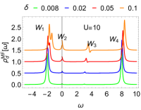
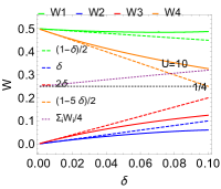
Figure 1: (Color online) (1) local electronic spectral functions for $\delta=0.008,~{}0.02,~{}0.05,~{}0.1$ with a $0.5$ shifting for each curve; (1) the spectral weights for each pole as a function of $\delta$ and compared with the corresponding asymptotic behaviors. Together shown is the average spectral weight $\sum_{i}W_{i}/4$ of the poles, which indicates approximate conservation of the total spectral weight (see text). A Lorentzian broadening factor $\eta^{+}=0.1$ is used in each curve in (1), and $\eta^{+}=0.01$ is used in (1).

Use the bare first order perturbation results, we identify that the poles of $\rho^{MF}_{d}[\omega]$ are approximately located at $\omega_{i}\in\{h-U/2,0,h,U/2+h\}$. The corresponding linear fittings for the spectral weight at these poles (dashed lines) are $\{(1-\delta)/2,~{}\delta,~{}2\delta,~{}(1-5\delta)/2\}$. These results clearly show that the poles respectively correspond to the $\{$lower Hubbard band, Fermi energy, mid-gap states, upper Hubbard band$\}$, and the spectral weight redistribution among them with doping. The spectral weight evolution is consistent with the analysis of CDMF results in Ref. [Sakai et al., 2009] blackwhen we take the doublon density to be $n_{doublon}=2\delta$ in our mean-field theory.

An interesting and important feature blackin the spectrum is the asymmetric structure of the pole $W_{2}$ about the Fermi level $\omega=0$. Though the jump of $\rho^{MF}_{d}[\omega]$ across $\omega=0$ is generally an artifact coming from treating the $f$-spinon density of states as a $\delta$-function, the asymmetry of the spectrum is a physical consequence of the pole of $G^{\alpha\bar{\alpha}^{\prime}}_{B,S}$. Note that, this is a zero frequency pole of a time-ordered Green’s function. Thus, it is a dynamical pole whose imaginary part should be interpreted as $\Im m[1/(\omega+i\delta\text{sgn}[\omega])]\propto\partial_{\omega}\delta(\omega)$. This pole contributes a component $\propto\partial_{\omega}\rho_{f}(\omega)$ to $\rho_{d}(\omega)$ after the convolution. Considering that the $f$-spinons are treated as canonical fermions whose self-energy is even in $\omega$, a dynamical particle-hole odd componentShastry (2012) blackaccounting for the asymmetric spectral weight should be incorporated in $\rho_{d}(\omega)$ through this pole, blackand this is an important hallmark of strong $U$ correlations in recent microscopic theories including the ECFL theoryShastry (2011, 2012), the hidden Fermi liquid theoryAnderson and Casey (2009); Casey and Anderson (2011), as well as DMFT resultsDeng et al. (2013); Xu et al. (2013).

Spin-spin interactions of the doped phase.   blackThe dynamical expansion allows us to extract the superexchange interactions in terms of the $f$-spinons

$$H_{J}=\frac{J_{ij}}{2}f^{\dagger}_{i\alpha}f_{i\beta}f^{\dagger}_{j\beta}f_{j\alpha}\Rightarrow J_{ij}\bm{S}_{i}\cdot\bm{S}_{j}.$$ (14)

Here $J_{ij}$ blackis obtained by contracting the vertex at one-loop levelDing et al. (2014) as

$$\begin{split}&J_{ij}=t_{ij}^{2}\int\frac{-d\omega}{2\pi}\sum_{ss^{\prime}ll^{\prime}}G^{+-}_{B,S,ss^{\prime}}[\omega,i,i]G^{-+}_{B,S,ll^{\prime}}[\omega,j,j].\end{split}$$ (15)

blackPlugging in the slave-spin Green’s function at the atomic limit, we find the superexchange interaction at half-filling: $J_{0}=2t_{ij}^{2}/U$. The missing factor of 2 can be restored blackwhen taking into account the fluctuations of the hopping term similar as in Ref. [Ding et al., 2014].

blackAt finite doping, more channels of spin-spin interactions arise from different dynamical processes, and they can be calculated term by term according to Eq. (15) and (9). Up to the leading orders,

$$J =J^{(0)}+J^{(1)}+\dots,$$ (16)

where $J^{(0)}=-t^{2}\int\frac{d\omega}{2\pi}G^{+-}_{B,S,0}G^{-+}_{B,S,0}$, and $J^{(1)}=-t^{2}\int\frac{d\omega}{2\pi}(G^{+-}_{B,S,1}G^{-+}_{B,S,0}+G^{+-}_{B,S,0}G^{-+}_{B,S,1}).$ $J^{(0)}$ is the superexchange interactions, which is still governed by the virtual transition between the LHB and UHB as $G^{+-(-+)}_{B,S,0}$ only have poles at $\omega_{1}$ and $\omega_{4}$. To the lowest order in $\delta$, we have

$$J^{(0)}\simeq J^{*}_{0}(1-2\delta)$$ (17)

where $a=h/U$ and $J_{0}^{*}=J_{0}(1-4a^{2})^{-1}$ which is the bare superexchange interaction strength if only the energy shifting of the LHB and UHB caused by doping is accounted for. $J^{(1)}$ is due to the virtual transitions between LHB and the mid-gap pole $W_{2}$. To the lowest order, we have

$$J^{(1)}\simeq-\frac{M_{x}^{2}t^{2}}{1+4a},$$ (18)

which is ferromagnetic. By extrapolation, we find $M_{x}^{2}\big{|}_{U\rightarrow\infty}\simeq\delta$, which indicates that at finite doping and in the $U\rightarrow\infty$ limit only the ferromagnetic interaction survives. This links to the Nagaoka ferromagnetismNagaoka (1966); Tasaki (1998).

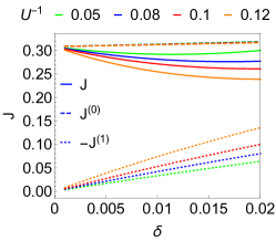
Figure 2: (i) the total spin-spin interactions strength $J$ (solid lines), (ii) the superexchange interaction strength $J^{(0)}$ (dashed lines) and (iii) the ferromagnetic interaction strength $(-1)\times J^{(1)}$ (dotted lines) plotted as functions of $\delta$.

Effective theory at first order in $t/U$.   Based on the above mean-field solution, we can further construct an effective theory for the doped HM in a way similar to Ref. [Ding et al., 2014]. The resulting theory contains Hamiltonians in both the slave-spin and $f$-spinon sectors

$$H_{S,eff}=H_{S,0}+H_{S,t},$$ (19)

$$H_{f,eff}=H_{f,t}+H_{f,0}+H_{J}.$$ (20)

$H_{f,eff}$ takes the form of a $t$-$J$ model and $H_{S,eff}$ takes the form of an XXZ spin model. They are dynamically coupled via self-consistent condition. In our theory the renormalization factors of $t$ and $J$ for the $f$-spinons, $g_{t}$ and $g_{J}$, are via the slave-spin correlations and no further Gutzwiller projection is necessary. Quantitatively we find

$$g_{t}=M_{x}^{2}=2\delta,\quad g_{J}=1-2\delta,$$ (21)

which agree well to those phenomenological values $g_{t}=2\delta/(1+\delta),\quad g_{J}=1/(1+\delta)^{2}$ first proposed by Zhang et. al. Zhang et al. (1988).

Conclusion.   In this work, we propose a slave-spin representation of the HM on a square lattice with nn hoppings and use the SEoM perturbation theory to implement a dynamical $t/U$ expansion in the doped MI. At the saddle-point level, our theory generates nontrivial dynamical properties of single-electron spectrum, including multiple pole structures and spectral weight (re-)distributions with doping, Both features are in excellent agreement with known numerical results despite that our theory is analytic in nature and works directly in the $\omega-\bm{k}$ space. blackWe also derive the exchange interactions among spins. In addition to the usual AFM superexchange interactions, we find a new FM channel at finite doping and finite $U$ values. This FM coupling survives the $U\rightarrow\infty$ limit and asymptotically connects to the Nagaoka ferromagnetism. It also provides a viable explanation for recently discovered FM orderSarkar et al. (2019) and spin fluctuationsSonier et al. (2010); Butch et al. (2012); Kurashima et al. (2018) in cuprates. In general, we find the low-energy effective theory of the doped MI is a dynamical $t$-$J$ model with effective renormalization factors in agreement with those proposed phenomenologically based on experimental data and empirical findings. Our theory thus provides a natural basis and reliable means in understanding the exotic properties of the doped HM.

Acknowledgement: We thank Q. Si for motivating this work, and J. Wu for useful discussions. The work at Anhui University was supported by the Startup Grant number S020118002/002 of Anhui University. WD thanks support from Kavli Institute for Theoretical Sciences. The work at Renmin University was supported by the National Science Foundation of China Grant number 11674392, the Fundamental Research Funds for the Central Universities and the Research Funds of Remnin University of China Grant number 18XNLG24, and the Ministry of Science and Technology of China, National Program on Key Research Project Grant number 2016YFA0300504.

Supplemental Materials

Solution of the slave-spin theory within Weiss mean-field approximation

In this part, we show the blacksaddle-point solution of the slave spin theory within a Weiss mean-field decomposition in Eq. (7) of the main text obtained by diagonalization.

First, we find the dMIMT blacktaking place at a finite $h_{c}$ with

$$h_{c}\simeq U/2\times\sqrt{U_{c}(U^{-1}_{c}-U^{-1})}.$$ (S1)

Note that in the single-orbital Hubbard model, one can always set $h=-\mu$, where $\mu$ is the electron chemical potential. This makes the ratio $a=h/U$ proportional to doping $\delta$, as shown in Figs. Fig. (blueSS1) and  Fig. (blueSS1). Actually,

$$a=a_{c}(1+b~{}\delta).$$ (S2)

blackwhere the factor $b$ decreases as $U$ increases, and the critical value $a_{c}=\sqrt{U^{-1}_{c}-U^{-1}}/2$.

The ratio black$a$ is shown for both its bare values in Fig. (blueSS1) and its changes from the critical point $a/a_{c}$ in Fig. (blueSS1). The change in $a$ as a percentage of $a_{c}$ is about 4 times of $\delta$, hence leads to the increase of $J_{0}$ as $\delta$ increases. We consider that it is an artifact of mean field theory since $h$ accounts also for effects due to the hopping terms.

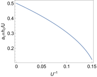
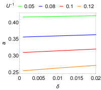
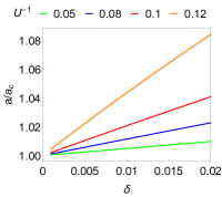
Figure S1: (blueSS1) bare values of $h$ shown at different $U$’s as functions of $\delta$; (blueSS1) $a_{c}=h_{c}/U$ shown as a function of $U^{-1}$ over the full range; (blueSS1) bare values of $a=h/U$; (blueSS1) the relative change of $a$ from $a_{c}$

The dMIMT is blackof Brinkman-Rice type, as we find that $Z\propto\delta$ which is shown in Fig. (blueSS2). To support the survival of the Nagaoka-ferromagnetic interaction in the $U\rightarrow\infty$ limit, we plot $Z/\delta$ as a function of $U^{-1}$. blackAs shown in Fig. (blueSS2), $Z/\delta$ converges to $1$ in the limit of $U\rightarrow\infty$, which indicates that the FM exchange coupling in Eq.(18) of the main text keeps finite in this limit.

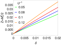
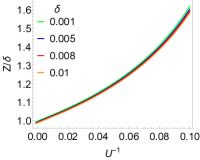
Figure S2: (blueSS2) $Z=M_{x}^{2}/2$ shown as functions of $\delta$ at different $U$’s; (blueSS2) $Z/\delta$ plotted as a function of $U^{-1}$ down to zero which converges to $1$.

Perturbative Schwinger’s equation-of-motion approach for quantum spins

A full description of the perturbative Schwinger’s equation-of-motion approach for spin-$1/2$ quantum spins is given in Ref. Ding, 2019 independently. Here we briefly present the approach and the solutions for the slave spins.

The Schwinger’s equation-of-motion theory converts the operator Heisenberg-equations-of-motion (HEoM) into equations of motion for the Green’s functions. For the quantum spins that blackobey the $SU(2)$ Lie-algebra, we introduce both a bosonic and a fermionic Green’s functions as the follows:

$$\begin{split}iG^{OO^{\prime}}_{\eta}[i,f]=\mbox{$\langle\langle\hat{O}_{i}[t_{i}]\hat{O}^{\prime}_{f}[t_{f}]\rangle\rangle$}_{\eta}=&\mbox{$\langle\mathcal{T}_{\pm}\left[\hat{O}_{i}[t_{i}]\hat{O}^{\prime}_{f}[t_{f}]\right]\rangle$}-C_{\eta}\mbox{$\langle\hat{O}_{i}\rangle$}\mbox{$\langle\hat{O}^{\prime}_{f}\rangle$}\\ =&~{}\mbox{$\langle\theta(t_{i}-t_{f})\hat{O}_{i}[t_{i}]\hat{O}^{\prime}_{f}[t_{f}]+\eta\theta(t_{f}-t_{i})\hat{O}^{\prime}_{f}[t_{f}]\hat{O}_{i}[t_{i}]\rangle$}-C_{\eta}\mbox{$\langle\hat{O}_{i}\rangle$}\mbox{$\langle\hat{O}^{\prime}_{f}\rangle$},\end{split}$$ (S3)

where $\eta=B,~{}F$ as subscripts while $\eta=\pm$ correspondingly in the equations and $C_{B(F)}=2(0)$. Whereas $G^{OO^{\prime}}_{B(F)}[i,f]$ are considered not independent, we consider both here since sometimes it is more convenient to use one not the other for computing certain quantities.

.1 Atomic limit solution

blackIn the atomic limit, since the slave spin Hamiltonian

$$H_{S,at}=\frac{U}{2}\sum_{i}(\sum_{s}S_{is}^{z})^{2}+h\sum_{is}S_{is}^{z}$$ (S4)

is purely Ising-type, we only need to consider

$$G^{\alpha\bar{\alpha^{\prime}}}_{\eta,S,ss^{\prime}}[i,f]=\mbox{$\langle\mathcal{T}[S_{is}^{\alpha}(t_{i})S_{fs^{\prime}}^{\bar{\alpha}^{\prime}}(t_{f})]\rangle$}-2\mbox{$\langle S_{is}^{\alpha}\rangle$}\mbox{$\langle S^{\bar{\alpha}^{\prime}}_{fs^{\prime}}\rangle$},$$ (S5)

with $\alpha=+$ or $-$.

First, we obtain the HEoM

$$-i\partial_{t}S^{\alpha}_{is}=[H_{int}^{S},S^{\alpha}_{is}]=\alpha US^{z}_{i\bar{s}}S^{\alpha}_{is}+\alpha hS^{\alpha}_{is}.$$ (S6)

Correspondingly, the SEoM is

$$-i\partial_{t_{i}}G^{\alpha\bar{\alpha^{\prime}}}_{B,S,\sigma\sigma^{\prime}}[i,f] =\alpha\left(2\mbox{$\langle S^{z}_{\sigma}\rangle$}\delta_{\alpha\alpha^{\prime}}\delta_{\sigma\sigma^{\prime}}\delta[i,f]-hG^{\alpha\bar{\alpha^{\prime}}}_{B,S,\sigma\sigma^{\prime}}[i,f]+J~{}\Gamma^{z\alpha;\bar{\alpha^{\prime}}}_{B,S,\bar{\sigma}\sigma;\sigma^{\prime}}[i,f]\right),$$ (S7)

$$-i\partial_{t_{i}}G^{\alpha\bar{\alpha^{\prime}}}_{F,S,\sigma\sigma^{\prime}}[i,f] =~{}\delta_{\alpha\alpha^{\prime}}\delta_{\sigma\sigma^{\prime}}\delta[i,f]+\alpha\left(-hG^{\alpha\bar{\alpha^{\prime}}}_{F,S,\sigma\sigma^{\prime}}[i,f]+J~{}\Gamma^{z\alpha;\bar{\alpha^{\prime}}}_{F,S,\bar{\sigma}\sigma;\sigma^{\prime}}[i,f]\right),$$ (S8)

where $\Gamma^{\alpha\alpha^{\prime};\alpha^{\prime\prime}}_{B(F)ss^{\prime};s^{\prime\prime}}[i,f]$ denotes the vertex functions defined as

$$i\Gamma^{\alpha\alpha^{\prime};\alpha^{\prime\prime}}_{B(F),S,ss^{\prime};s^{\prime\prime}}[i,f]=\mbox{$\langle\langle S^{\alpha}_{s}[t_{i}]S^{\alpha^{\prime}}_{s^{\prime}}[t_{i}]S^{\alpha^{\prime\prime}}_{\bm{s}^{\prime\prime}}[t_{f}]\rangle\rangle$}_{B(F)}.$$ (S9)

In the Ising limit, the vertex function can be simplified as

$$i\Gamma^{z\alpha;\alpha^{\prime}}_{B(F),S,ss^{\prime};s^{\prime\prime}}[i,f]=\mbox{$\langle S^{z}_{is}\rangle$}G^{\alpha\alpha^{\prime}}_{B(F),S,s^{\prime}s^{\prime\prime}}[i,f].$$ (S10)

To simplify the notation, we shall drop the slave spin index $s$ so that $G^{\alpha\bar{\alpha^{\prime}}}_{S}$ indicates a $2\times 2$ matrix. Here $\sigma_{i}$ denotes the Pauli matrices ($\sigma_{0}$ being the identity matrix). Denoting $\mbox{$\langle S^{z}_{a}+S^{z}_{b}\rangle$}=M,\ \mbox{$\langle S^{z}_{a}-S^{z}_{b}\rangle$}=m,$ which are good quantum numbers, we obtain

$$G^{\alpha\bar{\alpha^{\prime}}}_{B,S}[\omega]=\frac{\alpha\delta_{\alpha\alpha^{\prime}}(M\sigma_{0}+m\sigma_{z})}{\omega-\alpha(h+U(M\sigma_{0}-m\sigma_{z})/2)},$$ (S11)

$$G^{\alpha\bar{\alpha^{\prime}}}_{F,S}[\omega]=\frac{\delta_{\alpha\alpha^{\prime}}\sigma_{0}}{\omega-\alpha(+h+U(M\sigma_{0}-m\sigma_{z})/2)}.$$ (S12)

where inside the equation, $s=\pm 1$. blackWhat is $s$ here since $s$ has been just dropped?

Expressions for arbitrary states

For an arbitrary state $|\psi\rangle$, we can always expand it in terms of eigenstates of $H$. In this Ising limit, it is easy to prove that no crossing propagators for $\langle\langle S^{+}[t_{i}]S^{-}[t_{f}]\rangle\rangle$ and $\langle\langle S^{-}[t_{i}]S^{+}[t_{f}]\rangle\rangle$. Therefore, for any other states $|\psi(M,~{}m,~{}\Delta m)\rangle$ as given below,

$$\mbox{$|\psi_{M,m,\Delta m}\rangle$}=a\mbox{$|\uparrow\downarrow\rangle$}+b\mbox{$|\downarrow\uparrow\rangle$}+c\mbox{$|\uparrow\uparrow\rangle$}+d\mbox{$|\downarrow\downarrow\rangle$},$$ (S13)

where

$$M=c^{2}-d^{2},\quad m=a^{2}-b^{2},$$

$$\Delta m=\sqrt{\mbox{$\langle\hat{m}^{2}\rangle$}}=\sqrt{a^{2}+b^{2}}.$$ (S14)

We find that the arbitrary $G^{\alpha\alpha^{\prime}}_{B(F),para}$ can blackbe constructed as

$$\begin{split}&G^{\alpha\alpha^{\prime}}_{B(F),S,para}=\\ &a_{1}^{2}G_{B(F),S,M=1,m=0}+a_{2}^{2}G_{B(F),S,M=-1,m=0}\\ &+a_{3}^{2}G_{B(F),S,M=0,m=1}+a_{4}^{2}G_{B(F),S,M=0,m=-1},\end{split}$$ (S15)

where $para=(M,m,\Delta m)$ is the blackcomplete parameter set that describes the underlying state. With Eq. (S15), we can plug the $G_{B(F),S}$ back into the SEoM to obtain solutions for the vertex functions.

To prepare for the perturbation calculation of transverse field, we write down the explicit expressions for arbitrary states with physical parametrization (use $(M,~{}m,~{}\Delta m)$ instead of $a_{i}$s).

First, the solution for real $a_{i}$s blackis not unique. For later purpose, here we pick a solution that gives us a positive and uniform $\langle S^{x}\rangle$:

$$a_{1}=\sqrt{\frac{1+M-\Delta m^{2}}{2}},\quad a_{2}=\sqrt{\frac{1-M-\Delta m^{2}}{2}},$$ (S16)

$$a_{3}=\sqrt{\frac{m+\Delta m^{2}}{2}},\quad a_{4}=\sqrt{\frac{\Delta m^{2}-m}{2}},$$ (S17)

which gives

$$\begin{split}&\mbox{$\langle S^{x}_{a}\rangle$}=\mbox{$\langle S^{x}_{b}\rangle$}=1/2(\sqrt{\Delta m^{2}+m}\sqrt{1-\Delta m^{2}-M}\\ &+\sqrt{\Delta m^{2}-m}\sqrt{1-\Delta m^{2}+M}).\end{split}$$ (S18)

Now we can write Eq. (S15) as

$$\begin{split}&G^{\alpha\bar{\alpha}^{\prime}}_{B(F)}=\frac{1}{2}\Big{(}(1-\Delta m^{2})(G^{\alpha\bar{\alpha}^{\prime}}_{B(F),S,(1,0)}+G^{\alpha\bar{\alpha}^{\prime}}_{B(F),S,(-1,0)})\\ &+M(G^{\alpha\bar{\alpha}^{\prime}}_{B(F),S,(1,0)}-G^{\alpha\bar{\alpha}^{\prime}}_{B(F),S,(-1,0)})\\ &+m(G^{\alpha\bar{\alpha}^{\prime}}_{B(F),S,(0,1)}-G^{\alpha\bar{\alpha}^{\prime}}_{B(F),S,(0,-1)})\\ &+\Delta m^{2}(G^{\alpha\bar{\alpha}^{\prime}}_{B(F),S,(0,1)}+G^{\alpha\bar{\alpha}^{\prime}}_{B(F),S,(0,-1)})\Big{)},\end{split}$$ (S19)

where $(M,m)$ denotes the base states parameters.

The $G^{\alpha\alpha^{\prime}}_{B(F)}$ for arbitrary state with parameters $(M,\ m,\ \Delta m)$ read

$$G^{\alpha\bar{\alpha}}_{B,S,0}[\omega]=\frac{\alpha((1-\Delta m^{2})\sigma_{0}+m\sigma_{z})(\omega+\alpha h)+(M+\alpha\Delta m^{2})J\sigma_{0}/2}{(\omega+\alpha h)^{2}-U^{2}/4},$$ (S20)

$$G^{\alpha\bar{\alpha}}_{F,S,0}[\omega]=\frac{(\omega+\alpha h)\sigma_{0}+\alpha(M\sigma_{0}-m\sigma_{z})J/2}{(\omega+\alpha h)^{2}-U^{2}/4}.$$ (S21)

Weiss mean-field approximation to the hopping term of the slave spin Hamiltonian

In this part, we solve $H_{S,eff}$ for finite doping at the mean-field level. The mean-field approximation is to decouple $H_{S,hopping}$ as

$$\begin{split}&H_{S,hopping}\rightarrow H_{S,hMF}\\ &=-Q_{f}\sum_{is}\big{(}(\sum_{\mbox{$\langle ij\rangle$}s^{\prime}}\mbox{$\langle S^{-}_{js^{\prime}}\rangle$})S^{+}_{is}+h.c.\big{)},\end{split}$$ (S22)

Since the emergence of $\mbox{$\langle S_{is}^{\pm}\rangle$}\neq 0$ is from spontaneous-symmetry-breaking, we can choose the direction of the magnetization at our convenience: $\mbox{$\langle S^{+}_{is}\rangle$}=\mbox{$\langle S^{-}_{is}\rangle$}=\mbox{$\langle S^{x}_{is}\rangle$}=M_{x}$. On a 2D square lattice with only nearest neighbor (nn) hopping, $H_{S,MF}$ becomes

$$\begin{split}&H_{S,MF}=H_{S,at}+H_{S,hMF}\\ &=\sum_{i}\Big{(}US^{z}_{ia}S^{z}_{ib}+h(S^{z}_{ia}+S^{z}_{ib})-h_{x}(S^{x}_{ia}+S^{x}_{ib})\Big{)},\end{split}$$ (S23)

where $h_{x}=DM_{x}Q_{f}$, $D=4$ is the number of nn bonds for a two dimensional square lattice. This is a local Hamiltonian and can be solved by exact diagonalization. Here we adopt an alternative analytic calculation using a perturbation theory in terms of the Green’s functions.

The corresponding HEoM reads

$$-i\partial_{t}S^{\alpha}_{s}=\alpha(US^{z}_{\bar{s}}S^{\alpha}_{s}+hS^{\alpha}_{s}+h_{x}S^{z}_{s}),$$ (S24)

and hence the SEoM becomes

$$-i\partial_{t_{i}}G^{\alpha\bar{\alpha^{\prime}}}_{B,S,ss^{\prime}}[i,f] =\alpha\left(2\mbox{$\langle S^{z}_{s}\rangle$}\delta_{\alpha\alpha^{\prime}}\delta_{ss^{\prime}}\delta[i,f]-hG^{\alpha\bar{\alpha^{\prime}}}_{B,S,ss^{\prime}}[i,f]+J~{}\Gamma^{z\alpha;\bar{\alpha^{\prime}}}_{B,S,\bar{s}s;s^{\prime}}[i,f]+h_{x}G^{z\bar{\alpha^{\prime}}}_{B,S,\bar{s}s^{\prime}}[i,f]\right),$$ (S25)

$$-i\partial_{t_{i}}G^{\alpha\bar{\alpha^{\prime}}}_{F,S,ss^{\prime}}[i,f] =~{}\delta_{\alpha\alpha^{\prime}}\delta_{ss^{\prime}}\delta[i,f]+\alpha\left(-hG^{\alpha\bar{\alpha^{\prime}}}_{F,S,ss^{\prime}}[i,f]+J~{}\Gamma^{z\alpha;\bar{\alpha^{\prime}}}_{F,S,\bar{s}s;s^{\prime}}[i,f]+h_{x}G^{z\bar{\alpha^{\prime}}}_{F,S,\bar{s}s^{\prime}}[i,f]\right).$$ (S26)

According to the result of diagonalization, we know that the ground state is a singlet/triplet with the onset of an infinitesimal transverse field.

The effects of the perturbation term are twofold: i) modifying the ground state wavefunction(s); ii) altering the evolution of the states (altering the SEoM). So we first consider the change in wavefunction, which gives $G_{0}$ with renormalized parameters. Then we consider the revised SEoM hence the further correction to $G$’s and $\Gamma$’s.

In the presence of a transverse field $h_{x}\hat{x}$, a magnetization $M_{x,s}$ along the field direction is induced. Now with the new correlators $G^{z\bar{\alpha^{\prime}}}_{B(F)}$ entering the SEoM, we need to consider their HEoM and SEoM as well. The HEoM of $S^{z}_{s}$ reads

$$-i\partial_{t}S^{z}_{s}=ih_{x}S^{y}_{s}=\frac{h_{x}}{2}(S^{+}_{s}-S^{-}_{s}),$$ (S27)

which leads to the following SEoM in frequency space

$$\omega G^{z\bar{\alpha^{\prime}}}_{B}[\omega] =\frac{1}{2}(\alpha^{\prime}I_{x}+h_{x}\sum_{\alpha}\alpha G^{\alpha\bar{\alpha^{\prime}}}_{B}[\omega]),$$ (S28)

$$\omega G^{z\bar{\alpha^{\prime}}}_{F}[\omega] =\frac{h_{x}}{2}\sum_{\alpha}\alpha G^{\alpha\bar{\alpha^{\prime}}}_{F}[\omega],$$ (S29)

where the second equal sign is because we apply a uniform field along $\hat{x}$.

Note that

$$\begin{split}\mbox{$\langle S^{x}_{s}\rangle$}&=-i\mbox{$\langle[S^{z}_{s},S^{y}_{s}]\rangle$}=\frac{1}{2i}(G_{F}^{z+}[i,i]-G_{F}^{z-}[i,i])\\ =&-\int\frac{d\omega}{2\pi}\frac{h_{x}}{2i\omega}(G_{F,S,ss}^{++}[\omega]+G_{F,S,ss}^{--}[\omega]\\ &-G_{F,S,ss}^{-+}[\omega]-G_{F,S,ss}^{+-}[\omega]).\end{split}$$ (S30)

To the lowest order, the latter two terms can be computed as

$$\mbox{$\langle S^{x}_{s}\rangle$}=\int\frac{d\omega}{2\pi}\frac{h_{x}}{2i\omega}(G_{F,S,0,ss}^{-+}[\omega]+G_{F,S,0,ss}^{+-}[\omega]),$$ (S31)

where $G_{F,S,0,ss}^{-+}[\omega]$ is the Green’s function without transverse field in Eq. (S21).

The transverse magnetization, i.e. the quasiparticle weight, the magnetization, i.e. the hole density, and $\Delta m^{2}$ correction, to the lowest order in $h_{x}$, are found to be

$$\mbox{$\langle S^{x}_{a}\rangle$}\simeq h_{x}\left[\frac{U\sigma_{0}-2hM\sigma_{0}+2hm\sigma_{z}}{U^{2}-4h^{2}}\right]_{aa},$$ (S32)

$$M=2\mbox{$\langle S^{z}_{a}\rangle$}\simeq\frac{-4hh_{x}^{2}}{U(U^{2}/4-h^{2})},$$ (S33)

$$\delta\Delta m^{2}\simeq\frac{-h_{x}^{2}}{U^{2}/4-h^{2}}.$$ (S34)

which leads to $Z=M_{x}^{2}/2\propto\delta$ by solving the self-consistency equation $h_{x}=DM_{x}Q_{f}$. All are consistent with the numerical calculations.

In our SEoM theory, the dynamical spin Green’s functions of $H_{S,MF}$ can be written as

$$G^{\alpha\bar{\alpha^{\prime}}}_{B(F)}[\omega]\simeq G^{\alpha\bar{\alpha^{\prime}}}_{B(F),S,0}[\omega]+G^{\alpha\bar{\alpha^{\prime}}}_{B(F),S,1}[\omega],$$ (S35)

where $G^{\alpha\bar{\alpha^{\prime}}}_{B(F),S,1}[\omega]$ is the lowest order correction of $G^{\alpha\bar{\alpha^{\prime}}}_{B(F)}[\omega]$ (other than the change in the wavefunction under the evolution of $H_{0}$).

$$\begin{split}&G^{\alpha\bar{\alpha^{\prime}}}_{B,S,1,ss^{\prime}}[\omega]=\frac{\alpha}{\omega+\alpha h}\Big{(}\frac{\alpha^{\prime}(U\mbox{$\langle S^{x}_{s}\rangle$}+h_{x})I_{x}}{2}+\frac{Uh_{x}}{2\omega}\mbox{$\langle S^{x}_{s}\rangle$}\sum_{\alpha^{\prime\prime}}\alpha^{\prime\prime}G^{\alpha^{\prime\prime}\bar{\alpha^{\prime}}}_{B,S,0,\bar{s}s^{\prime}}[\omega]+\frac{h_{x}^{2}}{2\omega}\sum_{\alpha^{\prime\prime}}\alpha^{\prime\prime}G^{\alpha^{\prime\prime}\bar{\alpha^{\prime}}}_{B,S,0,ss^{\prime}}[\omega]\Big{)},\end{split}$$ (S36)

$$\begin{split}&G^{\alpha\bar{\alpha^{\prime}}}_{F,S,1,ss^{\prime}}[\omega]=\frac{\alpha}{\omega+\alpha h}\Big{(}\frac{Uh_{x}}{2\omega}M_{x}\sum_{\alpha^{\prime\prime}}\alpha^{\prime\prime}G^{\alpha^{\prime\prime}\bar{\alpha^{\prime}}}_{F,S,0,\bar{s}s^{\prime}}[\omega]+\frac{h_{x}^{2}}{2\omega}\sum_{\alpha^{\prime\prime}}\alpha^{\prime\prime}G^{\alpha^{\prime\prime}\bar{\alpha^{\prime}}}_{F,S,0,ss^{\prime}}[\omega]\Big{)}.\end{split}$$ (S37)