Background Subtraction using Adaptive Singular Value Decomposition

Abstract

An important task when processing sensor data is to distinguish relevant from irrelevant data. This paper describes a method for an iterative singular value decomposition that maintains a model of the background via singular vectors spanning a subspace of the image space, thus providing a way to determine the amount of new information contained in an incoming frame. We update the singular vectors spanning the background space in a computationally efficient manner and provide the ability to perform block-wise updates, leading to a fast and robust adaptive SVD computation. The effects of those two properties and the success of the overall method to perform a state of the art background subtraction are shown in both qualitative and quantitative evaluations.

1 Introduction

With static cameras, for example in video surveillance, the background, like houses or trees, stays mostly constant over a series of frames, whereas the foreground consisting of objects of interest, e.g. cars or humans, cause differences in image sequences. Background subtraction aims to distinguish between foreground and background based on previous image sequences and eliminates the background from newly incoming frames, leaving only the moving objects contained in the foreground. These are usually the objects of interest in surveillance.

1.1 Motivation

Data driven approaches are a major topic in image processing and computer vision, leading to state of the art performances, for example in classification or regression tasks. One example is video surveillance used for security reasons, traffic regulation, or as information source in autonomous driving. The main problems with data driven approaches are that the training data has to be well balanced and to cover all scenarios that appear later in the execution phase and has to be well annotated. In contrast to cameras mounted at moving objects such as vehicles, static cameras mounted at some infrastructure observe a scenery, e.g. houses, trees, parked cars, that is widely fixed or at least remains static over large amount of frames. If one is interested in moving objects, as it is the case in the aforementioned applications, the relevant data is exactly the one different from the static data. The reduction of the input data, i.e., the frames taken from the static cameras, to the relevant data, i.e., the moving objects, is important for several applications like the generation of training data for machine learning approaches or as input for classification tasks reducing false positive detections due to the removal of the irrelevant static part.

Calling the static part background and the moving objects foreground, the task of dynamic and static part distinction is known as foreground background separation or simply background subtraction.

1.2 Background Subtraction as Optimization Problem

Throughout the paper, we make the assumptions that the camera is static, the background is mostly constant up to rare changes and illumination, and the moving objects, considered as foreground, are small relative to the image size. Then background subtraction can be formulated as an optimization problem. Given an image sequence stacked in vectorized form into the matrix $A\in\mathbb{R}^{d\times n}$, with $d$ being the number of pixels of an image and $n$ being the number of images, foreground-background separation can be modeled as decomposing $A$ into a low-rank matrix $L$, the background and a sparse matrix $S$, the foreground, cf. Candes:RobustPCA . This leads to the optimization problem

$$\min_{L,S}\ \operatorname*{rank}(L)+\lambda\|S\|_{0}\quad\text{s.t.}\quad A=L+S.$$ (1)

Unfortunately, solving this problem is not feasible. Therefore, adaptations have to be made. Recall that a singular value decomposition (SVD) decomposes a matrix $A\in\mathbb{R}^{d\times n}$ into

$$A=U\Sigma V^{T}$$ (2)

with orthogonal matrices $U\in\mathbb{R}^{d\times d}$ and $V\in\mathbb{R}^{n\times n}$ and the diagonal matrix

$$\Sigma=\begin{bmatrix}\Sigma^{\prime}&\ 0\\ 0&\ 0\end{bmatrix}\in\mathbb{R}^{d\times n},\quad\Sigma^{\prime}\in\mathbb{R}^{r\times r},\qquad r=\operatorname*{rank}A,$$

where $\Sigma^{\prime}$ has strictly positive diagonal values. The SVD makes no relaxation of the rank, but, given $\ell\leq r$, the best (in an $\ell_{2}$ sense) rank-$\ell$, $\ell\in\mathbb{N}$, estimate $L$ of $A$ can be obtained by using the first $\ell$ singular values and vectors, see SVD_Approx ; SVD_History . This solves the optimization problems

$$\min\|A-L\|_{F}\text{~{}or~{}}\|A-L\|_{2}\quad\text{s.t.}\quad\operatorname*{rank}L\leq\ell.$$ (3)

We use the following notation throughout our paper: $U_{:,1:\ell}:={U(:,1:\ell)}:=[u_{1},...,u_{\ell}]$, with $u_{i}$ being the $i$-th column of U$,i\in\{1,...,\ell\}$.

The first $\ell$ columns of the $U$ matrix of the SVD (2) of $A$, i.e., the left singular vectors corresponding to the $\ell$ biggest singular values, span a subspace of the column space of $A$. The background of an image $J\in\mathbb{R}^{d\times 1}$ is calculated by the orthogonal projection of $J$ on $U_{\ell}:=U_{:,1:\ell}$ by $U_{\ell}(U_{\ell}^{T}J)$. The foreground then consists of the difference of the background from the image $J-U_{\ell}(U_{\ell}^{T}J)=\left(I-U_{\ell}U_{\ell}^{T}\right)J$.

The aim of a surveillance application is to subtract the background from every incoming image. Modeling the background via (3) results in a batch algorithm, where the low rank approximations are calculated based on some (recent) sample frames stacked together to the matrix $A$. Note that this allows the background to change slowly over time, for example due changing illumination or to parked cars leaving the scene. It is well–known that the computational effort to determine the SVD of $A$ with dimensions $d\gg n$ is $O(dn^{2})$ using R-SVD and computing only $U_{n}=U_{:,1:n}$ instead of the complete $d\times d$ matrix $U$, and the memory consumption is $O(dn)$, cf. Golub_van_Loan . Especially in the case of higher definition images, only rather few samples $n$ can be used in this way. This results in a dependency of the background model from the sample image size and an inability of adaption to a change in the background that is not covered in the few sample frames. Hence, a naive batch algorithm is not a suitable solution.

1.3 Main Contributions and Outline

The layout of this paper is as follows. In Sec. 2 we briefly revise related work in background subtraction and SVD methods. Sec. 3 introduces our algorithm of iteratively calculating a SVD. The main contribution here consists in the application and adaption of the iterative SVD to background subtraction. In Sec. 4 we propose a concrete algorithm that adapts the model of the background in a way that is dependent on the incoming data because of which we call it adaptive SVD. A straightforward version of the algorithm still has limitations, because of which we present extensions of the basic algorithm that overcome these deficits. In Sec. 5 evaluations of the method give an impression on execution time, generality, and performance capabilities of the adaptive SVD. Finally, in Sec. 6 our main conclusions are outlined.

2 Related Work

The “philosophical” goal of background modeling is to acquire a background image that does not include any moving objects. In realistical environments, the background may also change, due to influences like illumination or objects being introduced to or removed from the scene. Taking into account these problems as well as robustness and adaptation, background modeling methods can, according to the survey papers BOUWMANS_1 ; BOUWMANS_2 ; BOUWMANS_3 , be classified into the following categories: Statistical Background Modeling, Background Modeling via Clustering, Background Estimation and Neural Networks.

The most recent approach is, of course, to model the background via neural networks. Especially convolutional neural networks (CNNs) CNN have performed very well in may tasks of image processing. These techniques, however, usually involve a labeling of the data, i.e., the background has to be annotated, mostly manually, for a set of training images. The network then learns the background based on the labels. Background modeling is often combined with classification or segmentation tasks where every pixel of an image is assigned to one class. Based on the classes, the pixel can then be classified as background or foreground, respectively. Such techniques strongly depend on the trained data and besides new approaches like transfer learning (DeepLearning, , p. 526) or reinforcement learning ReinforcementLearning can only be improved by adding new data.

Statistical background modeling includes Gaussian models, support vector machines and subspace learning models. Subspace learning originates from the modeling of the background subtraction task as shown in (1). Our approach therefore also belongs to this domain. Principal Component Pursuit (PCP) Candes:RobustPCA is based on the convex relaxation of (1) by

$$\min_{L,S}\|L\|_{*}+\lambda\|S\|_{1}\quad\text{s.t.}\quad A=L+S,$$ (4)

with $\|L\|_{*}$ being the nuclear norm of matrix $L$, the sum of the singular values of $L$. The relaxation (4) can be solved by efficient algorithms such as alternating optimization. As PCP considers the $\ell_{1}$ error, it is more robust against outliers or salt and pepper noise than SVD based methods and thus more suited to situations that suffer of that type of noise. Since outliers are not a substantial problem in traffic surveillance which is our main application in mind, we do not have to dwell on this type of robustness. In addition, the pure PCP method also has its limitations such as being a batch algorithm, being computationally expensive compared to SVD, and maintaining the exact rank of the low rank approximation, cf. PCP_overview . This is a problem when it comes to data that is affected by noise in most components, which is usually the case in camera based image processing. We remark that to overcome the drawbacks of plain PCP, many extensions of the PCP have been introduced, see PCP_overview ; IncPCP_paper .

There is naturally a close relationship between our SVD based approach and incremental principal component analysis (PCA) due to the close relationship between SVD and PCA. Given a matrix $A\in\mathbb{R}^{n\times d}$ with $n$ being the number of samples and $d$ the number of features, the PCA searches for the first $k$ eigenvectors of the correlation matrix $A^{T}A$ which span the same subspace as the first $k$ columns of the $U$ matrix of the SVD of $A^{T}$, i.e., the left singular vectors of $A^{T}$. Thus, usually the PCA is actually calculated by a SVD, since $A^{T}=U\Sigma V^{T}$ gives $A^{T}A=U\Sigma V^{T}V\Sigma U^{T}=U\Sigma^{2}U^{T}$, the PCA produces the same subspace as our iterative SVD approach. One difference is that PCA originates from the statistics domain and the applications search for the main directions in which the data differs from the mean data sample. That is why the matrix $A$ usually gets normalized by subtraction of the columnwise mean and divided by the columnwise standard deviation before calculating the PCA which, however, makes no sense in our application. This is also expressed in the work by Ross et al. IncPCA , based on the sequential Karhunen-Loeve basis extraction from Seq_Kahrunen_Loeve . They use the PCA as a feature extractor for a tracking application. In our approach, we model the mean data, the background, by singular vectors only and dig deeper into the application to background subtraction, which we have not seen in works has not been considered in the PCA context. Nevertheless, we will make further comparisons to the PCA approach, pointing out further similarities and differences to our approach.

3 Update methods for rank revealing decompositions and applications

Our background subtraction method is based on an iterative calculation of an SVD for matrices augmented by columns, cf. Sauer19 . In this section we revise the essential statements and the advantages of using this method for calculating the SVD.

3.1 Iterative SVD

The method from Sauer19 is outlined, in its basic form, as follows:

• Given: SVD of $\mathbb{R}^{d\times n_{k}}\ni A_{k}=U_{k}\Sigma_{k}V_{k}^{T},n_{k}\ll d$, and $\operatorname*{rank}(A_{k})=:r_{k}$

• Aim: Compute SVD for $A_{k+1}=[A_{k},B_{k}],$
  $B_{k}\in\mathbb{R}^{d\times m_{k}},\ m_{k}:=n_{k+1}-n_{k}$

• Update: $A_{k+1}=U_{k+1}\Sigma_{k+1}V_{k+1}^{T}$ with
  

  $$U_{k+1}=U_{k}Q\begin{bmatrix}\tilde{U}&0\\ 0&I\end{bmatrix},$$

  $$V_{k+1}=\begin{bmatrix}V_{k}&0\\ 0&I\end{bmatrix}(P^{\prime}_{k}P_{k})^{T}\begin{bmatrix}\tilde{V}&0\\ 0&I\end{bmatrix},$$

  where $Q$ results from a QR-decomposition, $\Sigma_{k+1}$, $\tilde{U}$ and $\tilde{V}$ result from the SVD of a $(r_{k}+m_{k})\times(r_{k}+m_{k})$ matrix. $P_{k}$ and $P^{\prime}_{k}$ are permutation matrices.

For details, see Sauer19 . In the original version of the iterative SVD, the matrix $U_{k}$ is (formally) of dimension $d\times d$. Since in image processing $d$ captures the amount of pixels of one image, an explicit representation of $U_{k}$ consumes too much memory to be efficient which suggests to represent $U_{k}$ in terms of Householder reflections. This ensures that the memory consumption of the SVD of $A_{k}$ is bounded by $O(n_{k}^{2}+r_{k}d)$, and the step $k+1$ requires $O(n_{k+1}^{3}+d\,m_{k}(r_{k}+m_{k}))$ floating point operations.

3.2 Thresholding - Adaptive SVD

There already exist iterative methods to calculate an SVD, but for our purpose the approach from Sauer19 has two favorable aspects. The first one is the possibility to perform blockwise updates with $m_{k}>1$, that is, with several frames. The second one is the ability to estimate the effect of appending $B_{k}$ on the singular values of $A_{k+1}$. In order to compute the SVD of $A_{k+1}$, $Z:=U_{k}^{T}B_{k}$ is first calculated and a QR decomposition with column pivoting of $Z_{r_{k}+1:d,:}=QRP$ is determined. The $R$ matrix contains the information in the added data $B_{k}$ that is not already described by the singular vectors in $U_{k}$. Then, the matrix $R$ can be truncated by a significance level $\tau$ such that the singular values less than $\tau$ are set to zero in the SVD calculation of

$$\begin{bmatrix}\Sigma_{k}^{\prime}&Z_{1:r_{k},:}P^{T}\\ &R\end{bmatrix}.$$

Therefore, one can determine only from the (cheap) calculation of a QR decomposition, whether the new data contains significant new information and the threshold level $\tau$ can control how big the gain has to be for a data vector to be added to the current SVD decomposition in an iterative step.

4 Description of the Algorithm

In this section, we give a detailed description of our algorithm to compute a background separation based on the adaptive SVD.

4.1 Essential Functionalities

The algorithm in Sauer19 was initially designed with the goal to determine the kernels of a sequence of columnwise augmented matrices using the $V$ matrix of the SVDs. In background subtraction, on the other hand, we are interested in finding a low rank approximation of the column space of $A$ and therefore concentrate on the $U$ matrix of the SVD which will us allow to avoid computation and storage of $V$.

The adaptive SVD algorithm starts with an initialization step called SVDComp, calculating left singular vectors and singular values on an initial set of data. Afterwards, data is added iteratively by blocks of arbitrary size. For every frame in such a block, the foreground is determined and then the SVDAppend step performs a thresholding described in Sec. 3.2 to check whether the frame is considered in the update of the singular vectors and values that correspond to the background.

4.1.1 SVDComp

SVDComp performs the initialization of the iterative algorithm. It is given the matrix $A\in\mathbb{R}^{d\times n}$ and a column number $\ell$ and computes the best rank-$\ell$ approximation $A=U\Sigma V^{T}$,

$$U=:[U_{0},U_{0}^{\prime}]\text{, }\Sigma=:\begin{bmatrix}\Sigma_{0}&0\\ 0&\Sigma_{0}^{\prime}\end{bmatrix}\text{, }V=:[V_{0},V_{0}^{\prime}]\text{,}$$

by means of an SVD with $\Sigma_{0}\in\mathbb{R}^{\ell\times\ell},U_{0}\in\mathbb{R}^{d\times\ell}$, and $V_{0}\in\mathbb{R}^{n\times\ell}$. Also this SVD is conveniently computed by means of the algorithm from Sauer19 , as the thresholding of the augmented SVD will only compute and store an at most rank-$\ell$ approximation, truncating the $R$ matrix in the augmentation step to at most $\ell$ columns. This holds both for initialization and update in the iterative SVD.

As mentioned already in Sec. 3.1, $U_{0}$ is not stored explicitly but in the form of Householder vectors $h_{j},j=1,\dots,\ell$, stored in a matrix $H_{0}$. Together with a small matrix $\widetilde{U}_{0}\in\mathbb{R}^{\ell\times\ell}$ we then have

$$U_{0}=\widetilde{U}_{0}\prod_{j=1}^{\ell}(I-h_{j}h_{j}^{T}),$$

and multiplication with $U_{0}$ is easily performed by doing $\ell$ Householder reflection and then multiplication with an $\ell\times\ell$ matrix. Since $V_{0}$ is not needed in the algorithm it is neither computed nor stored.

4.1.2 SVDAppend

This core functionality augments a matrix $A_{k}$, given by $\widetilde{U}_{k},\Sigma_{k},H_{k}$, determined either by SVDComp or previous applications of SVDAppend, by $m$ new frames contained in the matrix $B\in\mathbb{R}^{d\times m}$ as described in Sec. 3.1. The details of this algorithm based on Householder representation can be found in Sauer19 . By the thresholding procedure from Sec. 3.2 one can determine, even before the calculation of the SVD, if an added column is significant relative to the threshold level $\tau$. This saves computational capacities by avoiding the expensive computation of the SVD for images that do not significantly change the singular vectors representing the background.

The choice of $\tau$ is significant for the performance of the algorithm. The basic assumption for the adaptive SVD is that the foreground consists of small changes between frames. Calculating SVDComp on an initial set of frames and considering the singular vectors, i.e., the columns of $U_{0}$, and the respective singular values gives an estimate for the size of the singular values that correspond to singular vectors describing the background. With a priori knowledge of the maximal size of foreground effects, $\tau$ can even be set absolutely to the size of singular values that should be accepted. Of course, this approach requires domain knowledge and is not entirely data driven.

Another heuristic choice of $\tau$ can be made by considering the difference between two neighboring singular values $\sigma_{i}-\sigma_{i+1}$, i.e., the discrete slope of the singular values. The last and smallest singular values describe the least dominant effects. These model foreground effects or small effects, negligible effects in the background. With increasing singular values, the importance of the singular vectors is growing. Based on that intuition, one can set a threshold for the difference of two consecutive singular values and take the first singular value exceeding the difference threshold as $\tau$. Fig. 1(d) illustrates a typical distribution of singular values. Since we want the method to be entirely data driven, we choose this approach. The threshold $\tau$ is determined by $\hat{i}:=\min\left\{i:\sigma_{i}-\sigma_{i+1}<\tau^{*}\right\}$ and $\tau=\sigma_{\hat{i}}$ with the threshold $\tau^{*}$ of the slope being determined in the following.

4.1.3 Re-initialization

The memory footprint at the $k$-th step in the algorithm described in Sec. 3.1 is $O(n_{k}^{2}+r_{k}\,d)$ and grows with every frame added in the SVDAppend step. Therefore, a re-initialization of the decomposition is necessary.

One possibility is to compute an approximation of $A_{k}\approx U_{k}\Sigma_{k}V_{k}^{T}\in\mathbb{R}^{d\times n_{k}}$ or the exact matrix $A_{k}$ by applying SVDComp to $A_{k}$ with a rank limit of $\ell$ that determines the number of singular vectors after re-initialization. This strategy has two disadvantages. The first one is that this needs $V_{k}$, which is otherwise not needed for modeling the background, hence would require unnecessary computations. Even worse, though $\widetilde{U}_{0}\in\mathbb{R}^{\ell\times\ell}$, $\Sigma_{0}\in\mathbb{R}^{\ell\times\ell}$, and $H_{0}\in\mathbb{R}^{d\times\ell}$ are reduced properly, the memory consumption of $V_{0}\in\mathbb{R}^{n_{k}\times\ell}$ still depends on the number of frames added so far.

The second re-initialization strategy, referred to as (II), builds on the idea of a rank-$\ell$ approximation of a set of frames representing mostly the background. For every frame $B_{i}$ added in step $k$ of the SVDAppend the orthogonal projection

$${U_{k}(:,1:\hat{i})}({U_{k}(:,1:\hat{i})}^{T}B_{i}),$$

i.e. the “background part” of $B_{i}$, gets stored successively. The value $\sigma_{\hat{i}}$ is determined in Sec. 4.1.2 as threshold for the SVDAppend step. If the number of stored background images exceeds a fixed size $\mu$, the re-initialization gets performed via SVDComp on the background images. No matrix $V$ is necessary for this strategy and the re-initialization is based on the background projection of the most recently appended frames.

In the final algorithm we use a third strategy, referred to as (III) which is inspired by the sequential Karhunen-Loeve basis extraction Seq_Kahrunen_Loeve . The setting is very similar and the $V$ matrix gets dropped after the initialization as well. The update step with a data matrix $B_{k}$ is performed just like the update step of the iterative SVD calculation in Sec. 3.1 based on the matrix $[U_{k}\Sigma_{k},B_{k}]$. The matrices $\Sigma_{k+1}$ and $U_{k+1}$ get truncated by a thresholding of the singular values at every update step. Due to this thresholding, the number of singular values and accordingly the number of columns of $U_{k}$ has an upper bound. Therefore, the maximum size of the system is fixed and no re-initialization is necessary. Calculating the SVD of $[U_{k}\Sigma_{k},B_{k}]$ is sufficient since due to

$$[U_{k}\Sigma_{k},B_{k}] [U_{k}\Sigma_{k},B_{k}]^{T}=U_{k}\Sigma_{k}\Sigma_{k}^{T}U_{k}^{T}+B_{k}B_{k}^{T}$$

$$=U_{k}\Sigma_{k}V_{k}^{T}V_{k}\Sigma_{k}^{T}U_{k}^{T}+B_{k}B_{k}^{T}$$

$$=[U_{k}\Sigma_{k}V_{k}^{T},B_{k}][U_{k}\Sigma_{k}V_{k}^{T},B_{k}]^{T}$$

the eigenvectors and eigenvalues of the correlation matrices with respect to $[U_{k}\Sigma_{k},B_{k}]$ and $[U_{k}\Sigma_{k}V_{k}^{T},B_{k}]$ are the same. Therefore, the the singular values of $[U_{k}\Sigma_{k},B_{k}]$ and $[U_{k}\Sigma_{k}V_{k}^{T},B_{k}]$ are the same, being roots of the eigenvalues of the correlation matrix. In our approach we combine the adaptive SVD with the re-initialization based on $U_{k}\Sigma_{k}$, i.e. we perform SVDComp on $U_{k}\Sigma_{k}$, because we want to keep the thresholding of the adaptive SVD. This is essentially the same as an update step in Karhunen-Loeve setting with $B_{k}=0$ and a more rigorous thresholding or a simple truncation of $U_{k}$ and $\Sigma_{k}$. The thresholding strategy of the adaptive SVD Sec. 3.2 is still valid, as the QR-decomposition with column pivoting sorts the columns of the matrix according to the $\ell_{2}$ norm and the columns of $U_{k}\Sigma_{k}$ are ordered by the singular values due to $||U\Sigma_{:,i}||_{2}=\sigma_{i}$. $U_{k}\Sigma_{k}$ already is in SVD form and therefore SVDComp at re-initialization is reduced to a QR decomposition to regain Householder vectors and a truncation of $U_{k}$ and $\Sigma_{k}$ which is less costly than performing a full SVD.

Since it requires the $V$ matrix, the first re-initialization strategy will not be considered in the following, where we will compare only the strategies (II) and (III).

4.1.4 Normalization

The concept of re-initialization via a truncation of $U_{k}$ and $\Sigma_{k}$ either directly through SVDComp of $U_{k}\Sigma_{k}$ or in the Karhunen-Loeve setting with thresholding of the singular values still has a flaw: the absolute value of the singular values grows with each frame appended to $U_{k}\Sigma_{k}$ as

$$\sum_{i=1}^{n}\sigma_{i}^{2}=\|A\|_{F}^{2}.$$

This also accounts for

$$\sum_{i=1}^{n_{k+1}}\sigma_{n_{k+1},i}^{2} =\|U_{k+1}\Sigma_{k+1}\|_{F}^{2}\approx\left\|[U_{k}\Sigma_{k},B_{k}]\right\|_{F}^{2}$$

$$=\|U_{k}\Sigma_{k}\|_{F}^{2}+\|B_{k}\|_{F}^{2}.$$

The approximation results from the thresholding performed at the update step. As only small singular values get truncated, the sum of the squared singular values grows essentially with the Frobenius norm of the appended frames. Growing singular values do not only introduce numerical problems, they also deteriorate thresholding strategies and the influence of newly added single frames decreases in later steps of the method. Therefore, some upper bound or normalization of the singular values is necessary.

Karhunen-Loeve Seq_Kahrunen_Loeve introduce a forgetting factor $\varphi\in[0,1]$ and update as $[\varphi\,U_{k}\Sigma_{k},B_{k}]$. They motivate this factor semantically: more recent frames get a higher weight. Ross et al. IncPCA show that this value limits the observation history. With an appending block size of $m$ the effective number of observations is $m/(1-\varphi)$. By the Frobenius norm argument, the singular values then have an upper bound. By the same motivation, the forgetting factor could also be integrated into strategy (III). Moreover, due to

$$\|(\varphi\,U_{k}\Sigma_{k})_{:,i}\|_{2}=\left\|\varphi\,\sigma_{i}\,U_{:,i}\right\|_{2}=\varphi\sigma_{i},$$

the multiplication with the forgetting factor keeps the order of the columns of $U_{k}\Sigma_{k}$ and linearly affects the 2-Norm and is thus compliant with the thresholding. However, the concrete choice of the forgetting factor in unclear.

Another idea for normalization is to set an explicit upper bound for the Frobenius norm of observations contributing to the iterative SVD, or, equivalently, to $\sum\sigma_{i}^{2}=\|A\|_{F}^{2}$. At initialization, i.e. at the first SVDComp, the upper bound is determined by $\frac{\|A\|_{F}^{2}}{n}\eta$ with $n$ being the number of columns of $A$ and $\eta$ being the predefined maximum size of the system. This upper bound is a multiple of the mean squared Frobenius norm of an input frame and we define a threshold $\rho:=\frac{\|A\|_{F}}{\sqrt{n}}\sqrt{\eta}$. If the Frobenius norm $\|\Sigma_{0}\|_{F}$ of the singular values exceeds $\rho$ after a re-initialization step, $\Sigma_{0}$ gets normalized to $\Sigma_{0}\frac{\rho}{\|\Sigma_{0}\|_{F}}$. One advantage of this approach is that the effective system size can be transparently determined by the parameter $\eta$.

In data science, normalization usually aims for zero mean and standard deviation one. Zero mean over the pixels in the frames, however leads to subtracting the row wise mean of $A$, replacing $A$ by $(I-11^{T})A$. This approach is discussed in incremental PCA, cf. IncPCA , but since the mean image usually contributes substantially to the background, it is not suitable in our application.

A framewise unit standard deviation makes sense since the standard deviation approximates the contrast in image processing and we are interested in the image content regardless of the often varying contrast of the individual frames. Different contrasts on a zero mean image can be seen as a scalar multiplication which also applies for the singular values. Singular values differing with respect to the contrast are not a desirable effect which is compensated by subtracting the mean and dividing by the standard deviation of incoming frames $B$, yielding $\frac{B-\mu}{\sigma}$. Due to the normalization of single images, the upper bound for the Frobenius norm $\rho$ is more a multiple of the Frobenius norm of an average image.

4.2 Adaptive SVD Algorithm

The essential components being described, we can now sketch our method based on the adaptive SVD in Alg. 1.

1

2

Data: Images of a static camera and a matrix $A$ of initialization images.

Result: Background and foreground images for every input image.

3

4$U,\Sigma,\hat{i}$ $\leftarrow$ SVDComp(A, $\ell$, $\tau^{*}$);

5 while there are input images do

6       B $\leftarrow$ read, vectorize, and normalize the current image;

7      

8      // project B onto the current background model;

9       J $\leftarrow$ $U_{:,1:\hat{i}}(U_{:,1:\hat{i}}^{T}\textnormal{{B}})$;

10      

11      // subtract the background from B and use this as mask on the input image;

12       F $\leftarrow$ $\textnormal{{B}}\,\cdot(|\textnormal{{B}}-\textnormal{{J}}|>\theta)$;

13      

14      // build a block of input images;

15       $M\leftarrow[M,\textnormal{{B}}]$;

16      

17      // append a block of images;

18       if $M.cols==\beta$ then

19            

20            $U,\Sigma,\hat{i}$ $\leftarrow$ SVDAppend($U$, $\Sigma$, M, $\tau^{*}$);

21             $M\leftarrow$ [ ];

22            

23       end if

24      

25      // re-initialization if maximum size is exceeded;

26       if $U.cols>n^{*}$ then

27            

28            $U,\Sigma$ $\leftarrow$ SVDComp($U\Sigma$, $\ell$);

29            

30       end if

31      

32 end while

Algorithm 1 Background Subtraction using adaptive SVD.

The algorithm uses the following parameters:

• $\ell$: Parameter used in SVDComp for rank-$\ell$ approximation.

• $\eta$: Parameter for setting up the maximal Frobenius norm as a multiple of the Frobenius norm of an average image.

• $\tau^{*}$: Threshold value for the slope of the singular values used in SVDAppend.

• $\theta$: Threshold value depending on the pixel intensity range to discard noise in the foreground image.

• $\beta$: Number of frames put together to one block $B_{k}$ for SVDAppend.

• $n^{*}$: Maximum number of columns of $U_{k}$. If $n^{*}$ is reached a re-initialization is triggered.

For the exposition in Alg. 1 we use pseudo-code with a MATLAB like syntax. Two further explanations are necessary, however. First, we remark that SVDAppend and SVDComp return the updated matrices $U$ and $\Sigma$ and the index of the thresholding singular value determined by $\tau^{*}$ as described in Sec. 4.1.2. Using the threshold value $\theta$, the foreground resulting from the subtraction of the background from the input image gets binarized. This binarization is used as mask on the input image to gain the parts that are considered as foreground. $|B-J|>\theta$ checks elementwise whether $|B_{jk}-J_{jk}|>\theta$ and returns a matrix consisting of the Boolean values of this operation.

4.3 Relaxation of the small foreground assumption

A basic assumption of our background subtracting algorithm is that the changes due to the foreground are small relative to the image size. Nevertheless, this assumption is easily violated, e.g. by a truck in traffic surveillance or generally by objects close to the camera which can appear in singular vectors that should represent background. This has two consequences. The first is that the foreground object is not recognized as such, the second one leads to ghosting effects because of the inner product as shown in Fig. 1.

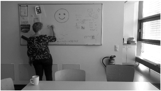
(a) Original image.

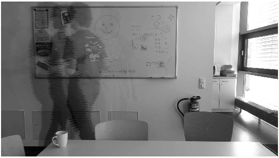
(b) Orthogonal projection onto background subspace.

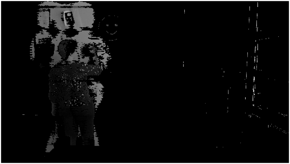
(c) Foreground image.

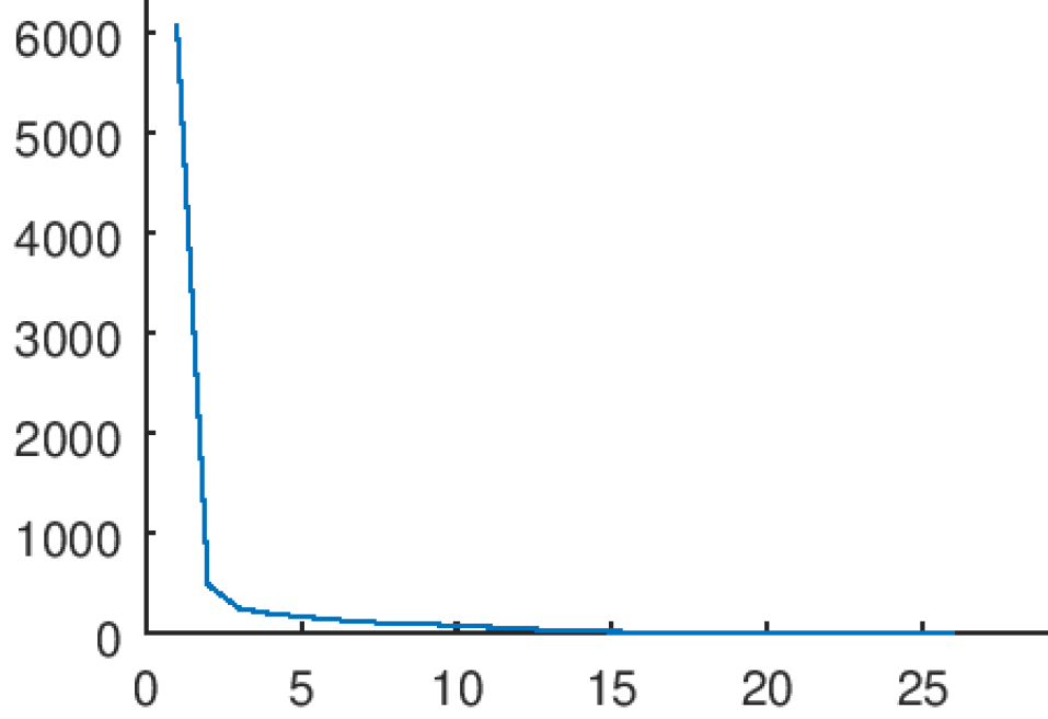
(d) Magnitude of the singular values plotted over the position on the diagonal of $\Sigma$.

Figure 1: Example of artifacts due to a big foreground object that was added to the background. The foreground object in the original image (a) triggers singular vectors containing foreground objects falsely added to the background (b) in previous steps. These artifacts can thus be seen in the foreground image (c).

The following modifications increase the robustness of our method against these unwanted effect.

4.3.1 Similarity Check

Big foreground objects can exceed the threshold level $\tau$ in SVDAppend and therefore are falsely included in the background space. With the additional assumption that background effects have to be stable over time, frames with large moving objects can be filtered out by utilizing the block appending property of the adaptive SVD. There, a large moving object causes significant differences in a block of images which can be detected by calculating the structural similarity of a block of new images. Wang et al. propose in SSIM the normalized covariance of two images to capture the structural similarity. This again can be written as the inner product of normalized images, i.e.,

$$s(B_{i},B_{j})=\frac{1}{d-1}\sum_{l=1}^{d}\frac{B_{i,l}-\mu_{i}}{\sigma_{i}}\frac{B_{j,l}-\mu_{j}}{\sigma_{j}},$$

with $B_{i}$ and $B_{j}$ being two vectorized images with $d$ pixels, means $\mu_{i}$, $\mu_{j}$ and standard deviations $\sigma_{i}$ and $\sigma_{j}$. Taking into account that the input images already become normalized in our algorithm, see Sec. 4.1.4, this boils down to a inner product.

Given is a temporally equally spaced and ordered block of images $B:=\{B_{1},B_{2},...,B_{m}\}$ and one frame $B_{i}$ with $i\in\{1,2,...,m\}=:M$. The structural similarity of frame $B_{i}$ regarding the block $B$ is the measure we search for. This can be calculated by

$$\frac{1}{m-1}\sum_{j\in M\setminus\{i\}}s(B_{i},B_{j}),$$

i.e., the mean structural similarity of $B_{i}$ regarding $B$. For the relatively short time span of one block it generally holds that $s(B_{i},B_{j})\geq s(B_{i},B_{k})$ with $i,j,k\in M$ and $i<j<k$, i.e., the structural similarity drops going further into the future as motions in the images imply growing differences. This effect causes the mean structural similarity of the first or last frames of $B$ generally being lower than of the middle ones due to the higher mean time difference to the other frames in the block.

This bias can be avoided by calculating the mean similarity regarding subsets of $B$. Let $\nu>0$ be a fixed number of pairs to be considered for the calculation of the mean similarity and $\Delta T\in\mathbb{N}^{+}$ be the fixed cumulative time difference. Calculate the mean similarity $\overline{s_{i}}$ of $B_{i}$ regarding to $B$ by selecting pairwise distinct $\{j_{1},j_{2},...,j_{\nu}\}$ from $M\setminus\{i\}$ with

$$\sum_{l=1}^{\nu}|j_{l}-i|=\Delta T\quad\text{and}\quad\overline{s_{i}}=\frac{1}{\nu}\left(\sum_{l=1}^{\nu}s(B_{i},B_{j_{l}})\right).$$

If $\overline{s_{i}}$ is smaller than the predefined similarity threshold $\overline{s}$, frame $i$ is not considered for the SVDAppend.

4.3.2 Periodic Updates

Using the threshold $\tau$ speeds up the iterative process, but also has a drawback: if the incoming images stay constant over a longer period of time, the background should mostly represent the input images and there should be high singular values associated to the singular vectors describing it. Since input images that can be explained well do not get appended anymore, this is, however, not the case. Another drawback is that outdated effects, like objects that stayed in the focus for quite some time and then left again, have a higher singular vectors than they should, as they are not relevant any more. Therefore, it makes sense to periodically append images although they are seen as irrelevant and do not surpass $\tau$. This also helps to remove falsely added foreground objects much faster.

4.3.3 Effects of the re-initialization strategy

The re-initialization strategy (II) based on the background images ${U_{k}(:,1:\hat{i})}({U_{k}(:,1:\hat{i})}^{T}B_{i})$ as described in Sec. 4.1.3 supports the removal of incorrectly added foreground objects. When such an object, say $X$, is gone from the scene, i.e., $B_{i}$ does not contain $X$ and ${U_{k}(:,1:\hat{i})}({U_{k}(:,1:\hat{i})}^{T}B_{i})$ does not contain it either because a singular vector not containing $X$ approximates $B_{i}$ much better. As $X$ was added to the background, there must be at least one column $j^{*}$ of $U_{k}$ containing $X$, i.e., ${U_{k}(:,1:j^{*})}^{T}X\gg 0$. As ${U_{k}(:,1:\hat{i})}({U_{k}(:,1:\hat{i})}^{T}B_{i})$ does not contain $X$, $({U_{k}(:,1:\hat{i})}^{T}B_{i})_{j^{*}}$ must be close to zero as otherwise the weighted addition of singular vectors ${U_{k}(:,1:\hat{i})}({U_{k}(:,1:\hat{i})}^{T}B_{i})$ cancels $X$ out. The re-initialization is thus based on images not containing $X$ and the new singular vectors also do not contain leftovers of $X$ anymore.

Finally, the parameter $\eta$ modifies the size of the maximum Frobenius norm used for normalization in re-initialization strategy (III) from Sec. 4.1.4. A smaller $\eta$ reduces the importance of the already determined singular vectors spanning the background space and increases the impact of newly appended images. If an object $X$ was falsely added, it gets removed more quickly if current frames not containing $X$ have a higher impact. A similar behavior like with re-initialization strategy (II) can be achieved. The disadvantage is that the background model changes quickly and does not capture long time effects that well. In the end, it depends on the application which strategy performs better.

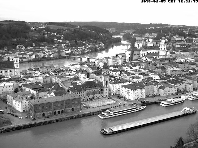
(a) Original image.

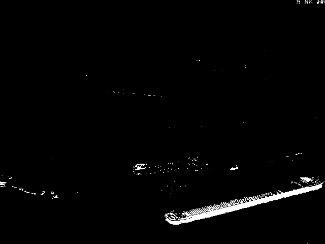
(b) Foreground image.

Figure 2: Example frame from a webcam video monitoring the city of Passau. In 2(a) the input image can be seen and in 2(b) the foreground image as a result of algorithm 1.

5 Computational Results

The evaluation of our algorithm is done based on an implementation in the C++ programming language using Armadillo Armadillo for linear Algebra computations.

5.1 Default Parameter Setting

Alg. 1 depends on parameters that are still to be specified. In the following, we will introduce a default parameter setting that works well in many different applications. The parameters could even be improved or optimized for a specific application using ground truth data. Our aim here, however, is to show that the adaptive SVD algorithm is a very generic one and applicable almost “out of the box” for various situations. The chosen default parameters are as follows:

• $\ell=15$,

• $n^{*}=30$,

• $\eta=30$,

• $\tau^{*}=0.05\cdot\rho$, with $\rho=\frac{||A||_{F}}{\sqrt{n}}\sqrt{\eta}$ of the initialization matrix $A$,

• $\beta=6$, $\nu=3$, $\Delta T=6$, $\overline{s}=0.97$,

• $\theta=1.0$.

The parameter $\ell$ determines how many singular values and corresponding singular vectors are kept after re-initialization. Setting $\ell$ too low can cause a loss of background information. In our examples, $15$ turned out to be sufficient not to lose information. The re-initialization is triggered when $n^{*}$ relevant singular values have been accumulated. Choosing that parameter too big reduces the performance, as the floating point operations per SVDAppend step depend cubically on the number of singular vectors and linearly on the number of singular vectors times the number of pixels, see Sec. 3.1. The system size $\eta$ controls the impact of newly appended frames, and a large value of $\eta$ favors a stable background. The threshold value $\tau^{*}$ for the discrete slope of singular values in the SVDAppend step depends on the data. The heuristic factor $0.05$ proved to be effective to indicate that the curve of the singular values flattens out. The block size $\beta$ and the corresponding $\nu$ and $\Delta T$ depend on the frame rate of the input. The choice is such that it does not delay the update of the background space too much, which would be the effect of a large block size. Keeping it relatively small, we are able to evaluate the input regarding similarity and stable effects. Due to the normalization of the input images to zero mean and standard deviation one, the similarity threshold $\overline{s}$ and the binarization threshold $\theta$ are stable against different input types.

5.2 Small Foreground Objects

The first example video for a qualitative evaluation is from a webcam monitoring the city of Passau, Germany, from above. The foreground objects, e.g. cars, pedestrians, boats, are small or even very small. The frame rate of 2 frames per minute is relatively low and the image size is $640\times 480\,$px. This situation allows for a straightforward application of the basic adaptive SVD algorithm without similarity check and regular updates. The remaining parameters are as in the default setting of Sec. 5.1.

In Fig. 2 an example frame and the according foreground image from the webcam video is shown. The moving boat in the foreground, the cars in the lower left and right corners, and even the cars on the bridge in the background are detected well. Small illumination changes and reparking vehicles lead to incorrect detections on the square in the front. Fig. 3 depicts these regions.

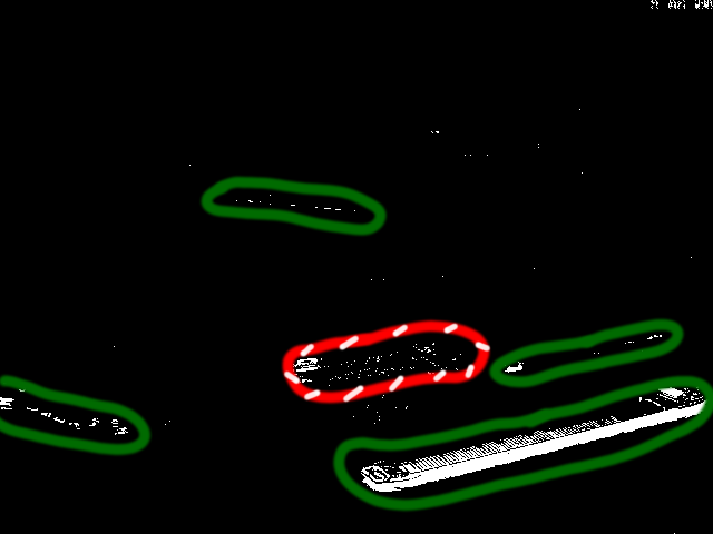
Figure 3: Plot marking the true detections in the foreground image of Fig. 2(b) by green circles and incorrect detections by red circles with white stripes.

5.3 Handling of Big Foreground Objects

(a) Original image.

(b) Orthogonal projection onto background subspace.

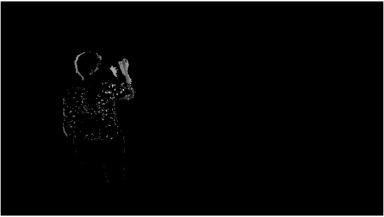
(c) Foreground image.

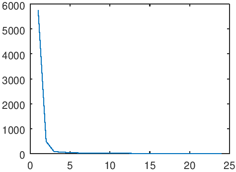
(d) Magnitude of the singular values plotted over the position on the diagonal of $\Sigma$.

Figure 4: The same scene as in Fig. 1. The artifacts due to big foreground objects are reduced by similarity checks and regular updates. The current foreground object gets added to the background only after being stationary for a series of frames.

Fig. 1 is a frame from an example video including the projection onto the background space, the computed foreground image, and the distribution of the singular values. To illustrate the improvements due to similarity checks and periodic updates, the same frame is depicted in Fig. 4 where the extended version of our algorithm is applied. The artifacts due to big foreground objects that were added to the background in previous frames, are not visible anymore. The person in the image still gets added to the background, but only after being stationary for some frames.

5.4 Execution Time

The performance of our implementation is evaluated based on an Intel® Core™ i7-4790 CPU @ $3.60\text{\,}\mathrm{Hz}$ $\times\ 8$. The example video from Sec. 5.3 has a resolution of $1920\times 1080\,$px with $25\,$fps. For the application of our algorithm on the example video, the parameters are set as shown in Sec. 5.1.

As the video data was recorded with $25\,$fps, there is no need to consider every frame for a background update, because the background is assumed to be constant over a series of frames and can only be detected considering a series of frames. Therefore, only every second frame is considered for a background update, while a background subtraction using the current singular vectors is performed on every frame. Our implementation with the settings from Sec. 5.1 handles this example video with $8\,$fps.

For surveillance applications it is important that the background subtraction is applicable in real time for which $8\,$fps are too slow. One approach would be to reduce the resolution. The effects of that will be discussed in the following section. Leaving the resolution unchanged, the parameters have to be adapted. Setting $\ell=10$ and $n^{*}=25$ significantly reduces the number of background effects that can be captured, but turns out to be still sufficient for this particular scene. The number of images considered for background updates can be reduced as well. Downsampling the frames by averaging over a window size of $8$ and setting $\ell=10$ and $n^{*}=25$ leads to a processing rate of $25\,$fps which is real time.

In Sec. 3.1 we pointed out that the number of floating point operations for an update step depends linearly on the number of pixels $d$ when using Householder reflections. A re-initialization step is computationally even cheaper, because only Householder vectors have to be updated. The following execution time measurements underline the theoretical considerations. Our example video is resized several times, 900 images are appended, and re-initialization is performed when $n^{*}$ singular vectors are reached. Tab. 1 shows the summed up time for the append and re-initialization steps during iteration for the given image sizes. The number $d$ of pixels equals $$2,073,600$=1920\cdot 1080$.

#Pixels	Append	Factor	Re-init.	Factor
$d$	$69.30\text{\,}\mathrm{s}$	1.90	$16.46\text{\,}\mathrm{s}$	1.37
$d/2$	$34.28\text{\,}\mathrm{s}$	1.88	$8.25\text{\,}\mathrm{s}$	1.38
$d/4$	$16.67\text{\,}\mathrm{s}$	1.83	$3.79\text{\,}\mathrm{s}$	1.26
$d/8$	$6.72\text{\,}\mathrm{s}$	1.47	$1.68\text{\,}\mathrm{s}$	1.12
$d/16$	$2.28\text{\,}\mathrm{s}$	1	$0.75\text{\,}\mathrm{s}$	1

Table 1: Execution time for performing a SVD update iteratively on 900 frames for different image sizes and $d=2073600=1920\cdot 1080$.

The factors $t_{d/i}/(t_{d/16}\cdot\frac{16}{i})$ with $i\in\{1,2,4,8,16\}$ and total append or re-initialization times $t_{d/i}$ are shown in Tab. 1 for image sizes $d/i$. These factors should be constant for increasing image sizes due to the linear dependency. Still, the factors keep increasing, but even less than a logarithmic order. This additional increase in execution time can be explained due to the growing amount of memory that has to be managed and caching becomes less efficient as with small images.

5.5 Evaluation on Benchmark Datasets

The quantitative evaluation is performed on example videos from the background subtraction benchmark data set CDnet 2014 CDnet14 . The first one is the pedestrians video belonging to the baseline category. It contains 1099 frames ($360\times 240$ px) of people walking and cycling in the public. An example frame can be seen in Fig. 5.

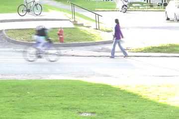
Figure 5: Example frame from the pedestrians video of the CDnet database.

For the frames 300 trough 1099 binary ground truth annotations exist that distinguish between foreground and background. From the first 299 frames, 15 frames are equidistantly sub-sampled and taken for the initial matrix $M$. Thereafter, Alg. 1 is executed on all frames from 300 through 1099. Instead of applying the binary mask in line 18 of algorithm 1 onto the input image, the mask itself is the output to achieve binary images.

	Recall	Specificity	FPR	FNR	PBC	Precision	F-Measure
default	0.869	1.000	0.000	0.131	0.158	0.967	0.915
morph	0.936	1.000	0.000	0.063	0.088	0.973	0.954

Table 2: Evaluation of the pedestrians scene of the CDnet database with the benchmark evaluation metrics including FPR (False Positive Rate), FNR (False Negative Rate), PBC (Percentage of Wrong Classifications).

With the default parameter setting of Sec. 5.1 a pixelwise precision of $0.958$ and an F-measure of $0.919$ are achieved with a performance of 843 fps. The thresholding leading to the binary mask is sensitive to the contrast of the foreground relative to the background. If it is low, foreground pixels are not detected properly. To avoid missing pixels within foreground objects, the morphological close operation is performed with a circular kernel. Moreover, a fixed minimal size of foreground objects can be assumed reducing the number of false positives. These two optimizations lead to a precision of $0.968$ and an F-measure of $0.958$ at $684$ fps. The complete evaluation measures can be seen in Tab. 2. Default represents the default parameter setting and morph the version with the additional optimizations. In the following, the morphological postprocessing is always included.

Our method delivers a state of the art performance for unsupervised methods. The best unsupervised method, IUTIS-5 IUTIS-5 on the benchmark site could achieve a precision of $0.955$ and an F-measure of $0.969$. It is based on genetic programming combining other state of the art algorithms. The execution time is not given, but naturally higher than the execution time of the slowest algorithm used, assuming perfectly parallel execution. We introduced domain knowledge only in the morphological optimizations. Otherwise, there is no specific change towards the test scene. Even more domain knowledge is used in supervised learning techniques as object shapes are trained and irrelevant movements in the background are excluded due to labeling. They are able to outperform our approach regarding the evaluation measures. An overall average precision and F-measure of more than $0.98$ is achieved. The benchmark site disclaims, nevertheless, that the supervised methods may have been trained on evaluation data as ground truth annotations are only available for evaluation data.

The positive effect of a block-wise appending of the data with a similarity check and regular updates as shown above also applies here: our adaptive SVD algorithm on the given pedestrians video from the benchmark site without using the similarity checks and regular updates only leads to a precision of $0.933$ and an F-measure of $0.931$.

The performance of our algorithm on more example videos from the CDnet data set is listed in Tab. 3. The park video is recorded with a thermal camera, the tram and turnpike videos with a low frame rate, and the blizzard video while snow is falling. For highway and park the best unsupervised method is IUTIS-5 and for tram, turnpike, blizzard, and streetLight that is SemanticBGS SemanticBGS . SemanticBGS combines IUTIS-5 and a semantic segmentation deep neural network and the execution time is given with 7 fps for $473\times 473\,$px images based on a NVIDIA GeForce GTX Titan X GPU.

Video	Prec	F-Meas	Prec*	F-Meas*
highway	0.901	0.816	0.935	0.954
park	0.841	0.701	0.776	0.765
tram	0.957	0.812	0.838	0.886
turnpike	0.962	0.860	0.980	0.881
blizzard	0.919	0.854	0.939	0.845
streetLight	0.992	0.982	0.984	0.983

Table 3: Evaluation of the adaptive SVD algorithm on example videos from the CDnet data set using precision and F-measure. Prec^∗ and F-Meas^∗ give the precision and F-measure of the best unsupervised method of the benchmark regarding to the test video.

Besides the park video, the content is mostly vehicles driving by. The performance of our algorithm clearly drops whenever the initialization image set contains a lot of foreground objects like in the highway video, where the street is never empty. Moreover, a foreground object turns into background when it stops moving which is even a feature of our algorithm. This, however, causes problems in a lot of the benchmark videos of the CDnet benchmark with vehicles stopping at traffic lights, like in the tram video, or people stopping and starting to move again. There is a category of videos with intermittent object motion in the CDnet data set. Our algorithm performs with an average precision of $0.752$ and an F-measure of $0.385$ whereas SemanticBGS reaches an average precision of $0.915$ and an F-measure of $0.788$. The precision of our algorithm tends to be higher than the F-measure, as it detects motion very well and therefore is certain that if there is movement, it is foreground, but often foreground is not detected due to a lack of motion. To delay the addition of a static object to the background, it is possible to reduce the regular updates, for example. But as this feature regulates the adaption of the background model to a change in the background, this only enhances the performance for very stable scenes. In the streetLight video no regular update was performed in contrast to the other videos. Including regular updates, the precision is $0.959$ and the F-measure $0.622$ due to cars stopping at traffic lights. The only domain knowledge we introduce is the postprocessing via morphological operations. Otherwise, the algorithm has no knowledge about the kind of background it models. Therefore, not only vehicles or people are detected as foreground, but also movement of trees or the reflection of the light of the vehicles on the ground, which is negative for the performance regarding the CDnet benchmark.

6 Conclusions

We utilized the iterative calculation of a Singular Value Decomposition to model a common subspace of a series of frames which is assumed to represent the background of the frames. An algorithm, the adaptive SVD was developed and applied for background subtraction in image processing. The assumption that the foreground has to be small objects was considered in more detail and relaxed by extensions of the algorithm. In an extensive evaluation, the capabilities of our algorithm were shown qualitatively and quantitatively using example videos and benchmark results. Compared to state of the art unsupervised methods we obtain competitive performance with even superior execution time. Even high definition videos can be processed in real time.

The evaluation also showed that, if an application to a domain such as video surveillance is intended, our algorithm would need to be extended to also consider semantic information. Therefore, it can only be seen as a preprocessing step, e.g. reducing the search space for classification algorithms. In future work we aim to evaluate the benefit of using our algorithm in preprocessing of an object classifier. Moreover, we will address the issue of foreground objects turning into background after being static for some time which is desirable in some cases and erroneous in others. A first approach is to use tracking, because objects do not disappear without any movement. In the end, there is also some parallelization ability in our algorithm separating the projection onto the background of incoming images from the update of the background model. Further performance improvements will be investigated.

- (1) Bianco, S., Ciocca, G., Schettini, R.: Combination of video change detection algorithms by genetic programming. IEEE Transactions on Evolutionary Computation 21(6), 914–928 (2017)
- (2) Bouwmans, T.: Recent advanced statistical background modeling for foreground detection: A systematic survey. Recent Patents on Computer Science 4, 147–176 (2011)
- (3) Bouwmans, T.: Traditional and recent approaches in background modeling for foreground detection: An overview. Computer Science Review 11-12, 31 – 66 (2014)
- (4) Bouwmans, T., Zahzah, E.H.: Robust pca via principal component pursuit: A review for a comparative evaluation in video surveillance. Computer Vision and Image Understanding 122, 22 – 34 (2014)
- (5) Bouwmans, T., ZAHZAH, E.h.: Robust pca via principal component pursuit: A review for a comparative evaluation in video surveillance. Computer Vision and Image Understanding 122, 22–34 (2014). DOI 10.1016/j.cviu.2013.11.009
- (6) Braham, M., Piérard, S., Van Droogenbroeck, M.: Semantic background subtraction. In: 2017 IEEE International Conference on Image Processing (ICIP), pp. 4552–4556 (2017)
- (7) Candès, E.J., Li, X., Ma, Y., Wright, J.: Robust principal component analysis? J. ACM 58(3), 11:1–11:37 (2011)
- (8) Golub, G.H., Van Loan, C.F.: Matrix Computations (3rd Ed.). Johns Hopkins University Press, Baltimore, MD, USA (1996)
- (9) Goodfellow, I., Bengio, Y., Courville, A.: Deep Learning. MIT Press (2016). http://www.deeplearningbook.org
- (10) LeCun, Y., Bottou, L., Bengio, Y., Haffner, P.: Gradient-based learning applied to document recognition. Proceedings of the IEEE 86, 2278–2324 (1998)
- (11) Levey, A., Lindenbaum, M.: Sequential karhunen-loeve basis extraction and its application to images. IEEE Transactions on Image Processing 9(8), 1371–1374 (2000)
- (12) Mnih, V., Kavukcuoglu, K., Silver, D., Rusu, A.A., Veness, J., Bellemare, M.G., Graves, A., Riedmiller, M., Fidjeland, A.K., Ostrovski, G., Petersen, S., Beattie, C., Sadik, A., Antonoglou, I., King, H., Kumaran, D., Wierstra, D., Legg, S., Hassabis, D.: Human-level control through deep reinforcement learning. Nature pp. 518–529 (2015)
- (13) Peña, J.M., Sauer, T.: Svd update methods for large matrices and applications. Linear Algebra and its Applications 561, 41 – 62 (2019)
- (14) Rodriguez, P., Wohlberg, B.: Incremental principal component pursuit for video background modeling. J. Math. Imaging Vis. 55(1), 1–18 (2016)
- (15) Ross, D.A., Lim, J., Lin, R.S., Yang, M.H.: Incremental learning for robust visual tracking. International Journal of Computer Vision 77(1), 125–141 (2008)
- (16) Sanderson, C., Curtin, R.: Armadillo: a template-based C++ library for linear algebra. The Journal of Open Source Software 1, 26 (2016)
- (17) Schmidt, E.: Zur Theorie der linearen und nichtlinearen Integralgleichungen. I. Teil. Entwicklung willkürlicher Funktionen nach Systemen vorgeschriebener. Math. Annalen 63, 433–476 (1907)
- (18) Stewart, G.W.: On the early history of the singular value decomposition. SIAM Rev. 35(4), 551–566 (1993)
- (19) Wang, Y., Jodoin, P., Porikli, F., Konrad, J., Benezeth, Y., Ishwar, P.: Cdnet 2014: An expanded change detection benchmark dataset. In: 2014 IEEE Conference on Computer Vision and Pattern Recognition Workshops, pp. 393–400 (2014)
- (20) Wang, Z., Bovik, A.C., Sheikh, H.R., Simoncelli, E.P.: Image quality assessment: from error visibility to structural similarity. IEEE Transactions on Image Processing 13(4), 600–612 (2004)