Effect of aggregation on adsorption phenomena

Abstract

Adsorption at an attractive surface in a system with particles self-assembling into small clusters is studied by Molecular dynamics (MD) simulation. We assume Lennard-Jones plus repulsive Yukawa tail interactions, and focus on small densities. The relative increase of the temperature at the critical cluster concentration near the attractive surface (CCCS) shows a power-law dependence on the strength of the wall-particle attraction. At temperatures below the CCCS, the adsorbed layer consists of undeformed clusters if the wall-particle attraction is not too strong. Above the CCCS, or for strong attraction leading to flattening of the adsorbed aggregates, we obtain a monolayer that for strong or very strong attraction consists of flattened clusters or stripes respectively. The accumulated repulsion from the particles adsorbed at the wall leads to a repulsive barrier that slows down the adsorption process, and the accession time grows rapidly with the strength of the wall-particle attraction. Beyond the adsorbed layer of particles, a depletion region of a thickness comparable with the range of the repulsive tail of interactions occurs, and the density in this region decreases with increasing strength of the wall-particle attraction. At larger separations, the exponentially damped oscillations of density agree with theoretical predictions for self-assembling systems. Structural and thermal properties of the bulk are also determined. In particular, a new structural crossover associated with the maximum of the specific heat, and a double-peaked histogram of the cluster size distribution are observed.

I Introduction

Theoretical studies and computer simulations show that competing interactions can lead to formation of spherical or elongated clusters, networks or layers of particles, and that these aggregates can form ordered periodic patterns at low temperature imperio:04:0 ; archer:07:1 ; archer:08:0 ; ciach:08:1 ; ciach:10:1 ; kowalczyk:11:0 ; zhuang:16:0 ; zhuang:16:1 ; edelmann:16:0 ; pini:17:0 . In experiment, three-dimensional (3D) periodic structures have not been detected yet, but the clusters and the network have been observed in a number of systems campbell:05:0 ; stradner:04:0 ; royall:18:0 ; bergman:19:0 . In these systems, the effective interactions between particles are attractive at short distances and repulsive at large distances (SALR). The repulsion is often of electrostatic origin, and the attraction can be induced by the (complex) solvent. Simulations of dilute systems reveal a structural crossover between individual particles (monomers) and clusters of a specific size. The borderline between the gas of particles at high temperature $T$ and small density $\rho$, and the gas of clusters at low $T$ and large $\rho$, was termed critical cluster concentration (CCC) santos:17:0 ; hu:18:0 . It resembles the critical micelle concentration line in amphiphilic systems amos:98:0 ; floriano:99:0 , and was defined in a similar way santos:17:0 .

Adsorption phenomenon has been intensely studied for many systems, because of its significance for various applications. To the best of our knowledge, however, the effect of aggregation and CCC on the adsorption and the near-surface structure has not been investigated yet. The two-dimensional models of particles interacting with the SALR potential show self-assembly into clusters, stripes and voids for increasing density imperio:04:0 ; archer:08:0 ; almarza:14:0 ; pekalski:14:0 . These results can give some information about the structure of the first layer of particles adsorbed at the surface. However, in the case of aggregation, the gas contains clusters that are 3D objects whose size and shape can be changed. When the attractive surface is in contact with such a gas, the adsorbed clusters can have different orientations and /or conformations, and different parts of them may occupy the first near-surface layer, therefore the 2D modeling can be an oversimplification. The questions whether the clusters are deformed near the surface, how they are distributed at different distances from the attractive wall, and how the aggregation influences the amount of adsorption for different strengths of wall-particle interactions are open.

In this work we investigate the near-surface structure in a system consisting of spherical particles interacting with the Lennard-Jones potential plus repulsive Yukawa tail. We choose the potential leading to formation of small clusters. Small clusters were observed for example in Ref.campbell:05:0 ; stradner:04:0 ; kowalczyk:11:0 ; bergman:19:0 . We do not focus on a particular system, but on a generic model that can reveal the general properties of adsorption in systems with competing interactions. We choose molecular dynamics (MD) simulations and study the structural properties both in the bulk and near an attractive surface.

In sec.2, we define the model and describe briefly the simulation method. In sec.3, we present the histograms for the cluster-size distribution, and determine the CCC temperature for three values of density in the bulk. This temperature will serve as a reference for the CCC in a vicinity of the surfaces (CCCS) with different strengths of particle-wall attraction. The pair distribution function is also determined in this section, and compared with theoretical predictions of the mesoscopic theoryciach:08:1 ; ciach:10:1 . In sec.4, we determine the effect of the wall-particle interaction strength on the temperature at the CCCS for three values of density. In addition, we determine the density profiles for several strengths of wall-particle interactions, and the adsorption in the near-surface layers of thickness $1.5\sigma$ and $2.6\sigma$, corresponding to a mono- and bilayer of particles at the wall, respectively. In sec. 5 we summarize and discuss our results.

II The model and the method

For the interaction potential we choose the sum of the short range Lennard-Jones (LJ) and the long range Yukawa potentials:

$$u(r)=6\epsilon\Bigg{[}\Bigg{(}\frac{\sigma}{r}\Bigg{)}^{12}-\Bigg{(}\frac{\sigma}{r}\Bigg{)}^{6}\Bigg{]}+\frac{A}{r}e^{-r/\xi}$$ (1)

where $\epsilon$ and $\sigma$ set the energy and length units, and we assume $A=1.8$ and $\xi=2$. The dimensionless temperature is defined as $T^{*}=k_{B}T/\epsilon$, where $k_{B}$ is the Boltzmann constant. For clarity, the asterisk will be omitted. The potential (1) is shown in Fig.1. The repulsion plays an important role in the SALR systems, therefore in simulations the potential was truncated at a relatively large distance $r=6.75\sigma$, for which the interaction potential is very small ($u(r)<0.009$ for $r>6.75$). We have performed additional test simulations for the cutoff $r=8$, and we got essentially the same results, with only a slight shift of the second maximum of the pair distribution function $g(r)$.

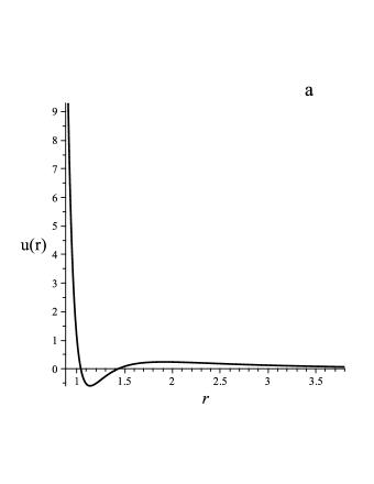
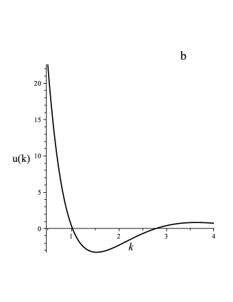
Figure 1: The interaction potential $u(r)$ defined in (1) in the real space (a), and the Fourier transform $\tilde{u}(k)$ of $\theta(r-1)u(r)$ (b). $r$ and $k$ are in $\sigma$ and $1/\sigma$ units, respectively. The symbol indicates $r=r_{cs}$, the cutoff distance such that a particle separated by $r<r_{cs}$ from its neighbor belongs to the same cluster.

To model the bulk, we consider $N=8000$ particles in a cubic box with periodic boundary conditions in all three directions. The simulations were performed applying the constant temperature and volume method litniewski:93:0 . We used this less known method because it is very simple and generates canonical distribution in the coordinate space without using additional variables and parameters (see also Ref.morishita:03:0 ; collins:10:0 ). The method is easy to implement by adopting the computer program used for classical constant energy and volume simulations. We focus on three values of the particle density, $\rho=0.0005,0.0015,0.005$, and fix the length $L$ of the edges of the cube accordingly.

In order to study the effect of the wall, the simulations were performed using the classical constant energy and volume method allen:90:0 for $N=12800$ particles in a rectangular box of the edges $L_{x}=L_{y}=L$ and $L_{z}\approx 1.6L$. The periodic boundary conditions are applied only along the $x$ and $y$ directions. The $z$-th direction is restricted by two walls. For the left wall we assume the wall-particle interaction of the form

$$V_{L}(z)=4\gamma\epsilon\Bigg{[}\Bigg{(}\frac{\sigma}{z-z_{L}}\Bigg{)}^{12}-\Bigg{(}\frac{\sigma}{z-z_{L}}\Bigg{)}^{6}\Bigg{]}$$ (2)

and for the right wall we assume only the repulsive interactions

$$V_{R}(z)=0.5\epsilon\Bigg{(}\frac{\sigma}{z_{R}-z}\Bigg{)}^{12},$$ (3)

where $z_{R}-z_{L}=1.6L$. We shall investigate the structure near the left wall for the range of attractive interaction $0.5<\gamma<3$.

In order to study the aggregation, we first introduce the distance criterion for particles forming the cluster. For the SALR potential, the distance $r=r_{cs}$, where the pair potential (1) crosses zero for the second time (see Fig.1a) is a natural distance such that a particle separated by $r<r_{cs}$ from a particle belonging to a cluster, belongs to the same cluster. The cluster size distribution is defined in the some way as in Ref.santos:17:0 ,

$$p(M)=\frac{MP(M)}{\sum_{M}MP(M)},$$ (4)

where $P(M)$ is the probability of finding an aggregate of size $M$.

The CCC is a structural crossover, and cannot be defined in a unique way. We adopt the criterion that the borderline between the monomers and the clusters is given by the inflection point at the $p(M)$ line defined in (4).

In contrast to thermodynamic phase transitions, the CCC is a structural crossover, and the CCC line is not uniquely defined. In fact the CCC is a crossover region rather than a line. We choose the inflection point of $p(M)$ defined in (4), because it is a well-defined borderline between the histograms with one maximum (for monomers) and two maxima (for the monomers and the optimal clusters). A maximum of the histogram for a particular size of the cluster indicates that there exists an optimal size, thus signaling formation of a well-defined structure rather than random inhomogeneities in the system. Different criteria for the CCC would lead only to some small shifts of our line within the crossover region.

III results for the bulk

III.1 the clusters

Simulation snapshots and the histograms (4) show formation of small clusters consisting of a few particles. For such a discrete system, we determine the temperature at the CCC from the first appearance of $p(M)/p(M-1)>1$ when the temperature is decreased. In our case it happens for $M=4$ for the three considered densities. Analyzing $p(4)/p(3)$ as a function of $T$ for $\rho=0.0005,0.0015,0.005$, we estimated $T_{CC}$ (here, the moment that $p(4)/p(3)=1$) as: $T=0.130,0.143,0.164$ for $\rho=0.0005,0.0015,0.005$ respectively.

The histograms for $\rho=0.005$ and $0.09<T<0.18$ are shown in Fig.2. At high $T$, $p(M)$ decreases monotonically, and for $T<0.164$ a maximum at $M=5$ appears. Further decrease of $T$ below $T=0.12$ leads to a second maximum for $M=7$. Clusters composed of more than $9$ particles are not formed, i.e. the distances between the particles within the cluster are smaller than the cutoff of the interaction potential, so our analysis is not biased by the choice of the cutoff.

It is interesting to find the energetically favorable structure of the clusters. The structures corresponding to the minimum energy per particle should form for very low T. In order to determine the structure of the clusters for $T\to 0$, we decreased the temperature of the system from $T=0.11$ (red line in Fig. 2b) to $T=0.0025$. From the distribution of the interparticle distances we find that in the 5 and 7 particle clusters, shown in Fig.3 , 3 and 5 particles form vertices of a regular triangle and pentagon with the edge length $a$, respectively. The two remaining particles are located above and below the center of the polygon at the line perpendicular to the polygon plane. They are separated by $2a\sqrt{2/3}$ and $a$ for the 5 and 7 particle cluster respectively.

For $M=5$, there is 9 pairs separated by the distance $a\approx r_{min}=1.139$, and one pair of particles separated by $2a\sqrt{2/3}$. The energy per particle is $U(5)/5\approx-1.03$. For $M=7$, $a\approx 1.007r_{min}$, and there are 6 pairs separated by $a$, 10 pairs separated by $~{}0.99a$ and 5 pairs separated by $~{}1.62a$, which gives the lowest energy per particle, $U(7)/7\approx-1.21$.

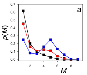
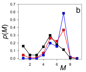
Figure 2: Histograms for the probability of finding a particle in a cluster consisting of $M$ particles for $\rho=0.005$. From the top to the bottom line on the left (black, red, blue), $T=0.18,0.16,0.14$ and $T=0.13,0.11,0.09$ on the (a) and (b) panels respectively. Lines are to guide the eye.

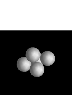
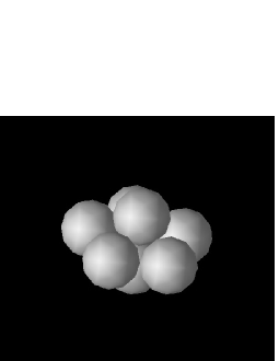
Figure 3: Cartoon showing the clusters composed of 5 and 7 particles, corresponding to the maxima of the histograms.

The instantaneous thermal structures differ from the ones corresponding to the minimum of the energy due to the thermal motion and entropic effects that depend strongly on temperature. In particular, deformations of the bigger, 7-fold clusters due to thermal motion of particles may lead to instantaneous configurations corresponding to the repulsion of some particles from the cluster, and to formation of smaller clusters, as we indeed observe. Our results indicate that the 5-fold clusters are more stable against the thermal motion, despite higher energy per particle in the optimal configuration. Only at low $T$, i.e. when the thermal motion is suppressed, the dominating clusters correspond to the lowest energy per particle, and for $T\to 0$ only the 7-particle clusters remain.

The fact that the 5-fold clusters dominate at high $T$ even though the 7-fold clusters have a lower energy in their optimal configuration is somewhat surprising. From the thermodynamic point of view, the reason is a fine balance between the energy $U$ and the entropy $S$ in the Helmholtz free energy $F=U-TS$. When the 7-fold clusters are formed, the number of objects (particles + clusters) decreases more strongly and it leads to a larger decrease of the entropy $S$ compared to the formation of the 5-fold clusters. At relatively high $T$ this effect may dominate over the increase of the energy (that is not large, especially for clusters deformed by thermal motion), therefore the 5-fold clusters may appear with higher probability than the 7-fold ones.

III.2 the pair distribution function

The pair distribution function $g(r)$ for $\rho=0.005$ and temperatures $T=0.11,0.13,0.15$ and $T=0.18$ is shown in Fig.4 for large separations $r>6$. The solid lines in Fig.4 were obtained by fitting the simulation results to the formula ciach:08:1 ; ciach:10:1 that in general should be obeyed asymptotically for $r\to\infty$,

$$g(r)=1+\frac{A_{0}}{r}\sin(\alpha_{1}r+\phi)e^{-\alpha_{0}r}.$$ (5)

The fitting parameters are given in table 1.

$T$	$\alpha_{1}^{f}$	$\alpha_{0}^{f}$	$\alpha_{1}^{t}$	$\alpha_{0}^{t}$	$\bar{M}$	$2\pi/\ell$
0.11	0.785	0.46	0.864	0.468	4.68	0.64
0.13	0.827	0.50	0.849	0.535	2.94	0.75
0.15	0.861	0.55	0.820	0.638	1.88	0.871
0.18	0.971	0.75	0.764	0.792	1.30	0.984

Table 1: Fitting parameters $\alpha_{0}^{f}$ and $\alpha_{1}^{f}$ for $g(r)$ approximated by Eq.(5) and shown in Fig.4. The parameters $\alpha_{1}^{t}$, $\alpha_{0}^{t}$ are obtained from the mesoscopic theory, Eq.(7), and $\bar{M}$ is the average number of particles per cluster obtained form the histograms. In the last column, $2\pi/\ell$, where $\ell$ is the average distance between the objects ($\ell^{3}=\bar{M}/\rho$) is shown. $T$ denotes temperature.

Eq.(5) fits the simulation results reasonably well for $r>6$, i.e. beyond the first period of the oscillatory decay. The satisfactory agreement between our numerical results for $g(r)$ and the analytical expression (5) that is valid only for distances larger than the range of the interactions confirms again that cutting off the interactions for $r=6.75$ is justified.

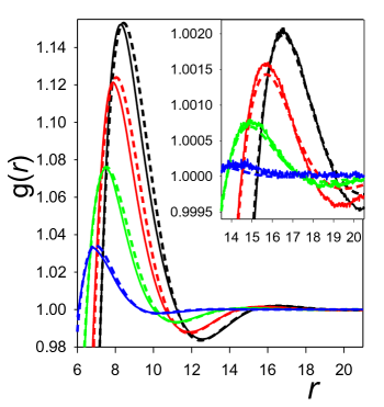
Figure 4: Pair distribution function $g(r)$ for $\rho=0.005$ and $T=0.11$ (black line), $T=0.13$ (red line), $T=0.15$ (green line) and $T=0.18$ (blue line). The dotted lines are the simulation results, and the continuous lines are the best fits to Eq.(5).

The fitting parameters can be compared with theoretical predictions of the mesoscopic density functional theory (DFT). In this mean-field (MF) theory ciach:08:1 ; ciach:10:1 , the Fourier transform $\tilde{G}(k)$ of $G(r)=(g(r)-1)\rho^{2}$ is approximated by

$$\tilde{G}(k)^{-1}=\beta\tilde{u}(k)-\frac{\partial^{2}s/k_{B}}{\partial\rho^{2}},$$ (6)

where $\beta=1/(k_{B}T)$, $s$ denotes the entropy per unit volume, and $\tilde{u}(k)$ denotes the Fourier transform of $u(r)\theta(r-1)$, where $u(r)$ is the interaction potential (Eq.(1)), and $\theta$ is the unit step function. With this definition of $\tilde{u}(k)$, we do not take into account contributions to the internal energy from overlapping cores of the particles. For the considered dilute systems, the perfect gas approximation, $s/k_{B}=-\rho(\ln(\rho)-1)$, is sufficiently accurate for homogeneous gases. When some fraction of the particles aggregates into clusters, however, then the number of objects - isolated particles plus clusters - is smaller than the number of particles. When the number of objects in the dilute system decreases, the entropy decreases as well. In a very crude approximation, we can consider a perfect gas of $N/\bar{M}$ objects, where $\bar{M}$ is the average number of particles per cluster. In this approximation,

$$\tilde{G}(k)^{-1}=\beta\tilde{u}(k)+\frac{1}{\bar{M}\rho}.$$ (7)

As shown in the histograms and table 1, $\bar{M}$ depends on temperature.

For the potential (1), $\tilde{G}(k)^{-1}$ takes a minimum for $k=k_{0}>0$ (Fig1). In such a case, in the real space representation we obtain the approximation, valid for large separations ciach:08:1 ; ciach:10:1

$$G(r)=\frac{A_{0}\rho^{2}}{r}\sin(\alpha_{1}r+\phi)e^{-\alpha_{0}r}$$ (8)

where $\alpha_{1}+i\alpha_{0}$ is the pole of $\tilde{G}(k)$ in the upper half of the complex $k$-plane with the smallest imaginary part and positive real part. The values of $\alpha_{0}$ and $\alpha_{1}$ depend significantly on the approximation for the entropy, and assuming the rather crude approximation in the MF theory, we cannot expect quantitative agreement with simulations. Still, a semiquantitative agreement is obtained for $\alpha_{0}$ that increases with $T$ in both theory and simulations. Neglecting the effect of clustering and assuming the perfect gas approximation for the entropy, leads to much poorer agreement with simulations, especially for low $T$, where a large fraction of particles belongs to the clusters. In particular, assuming the perfect gas entropy for $T=0.11$, we obtain $\alpha_{1}=0.792$ and $\alpha_{0}=0.719$. $\alpha_{1}$ obtained in this MF theory agrees semiquantitatively with simulations, but decreases with $T$, in contrast to the simulation results. In table 1, we also present $2\pi/\ell$, where $\ell$ is the average distance between the objects defined simply by $\ell^{3}=\bar{M}/\rho$. It is interesting to compare $\alpha_{1}$ and $2\pi/\ell$, because $2\pi/\alpha_{1}$ describes the distance between the maxima of $g(r)$. For high $T$, $\alpha_{1}^{f}$ and $2\pi/\ell$ agree quite well, while for lower $T$, when the systems gets more ordered, the distance between the maxima of $g(r)$ is smaller than the average distance between the objects. We conclude that fluctuations neglected in the MF theory influence the values of the parameters obtained from (7), but the formula (5) is a good approximation already for separations larger than the period of the damped density oscillations.

Finally, we investigated the effect of clustering on the deviation of the specific heat form the perfect gas form. As shown in Fig.5 for $\rho=0.005$, $c_{V}-3k_{B}/2$ takes a maximum for $T\approx 0.14$. For this temperature, $p(1)\approx p(5)$ (see Fig.2). One can expect the largest fluctuations of the energy when the probability that a particle is isolated or belongs to a cluster of the preferable size is the same. The temperature $T_{c_{V}}$ corresponding to the maximum of $c_{V}$ is a borderline between dominating isolated particles ( $p(1)>p(5)$) and dominating clusters ($p(1)<p(5)$), above and below $T_{c_{V}}$, respectively. The CCC temperature defined as the first appearance of nonmonotonic $p(M)$ upon decreasing $T$ is significantly higher. Below $T_{CC}$ the clusters are formed, but the monomers still dominate over the clusters until $T$ is decreased below $T_{c_{V}}$.

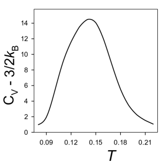
Figure 5: $c_{V}-3k_{B}/2$, where $c_{V}$ is the specific heat, for $\rho=0.005$ as a function of temperature $T$.

The presence of a maximum in $c_{V}$ recalls the maxima associated with a thermodynamic transition. In Ref.godfrin:14:0 it is shown that there is a correspondence between the clustering region and the two-phase region of a reference fluid in which the long-range repulsion is absent. In the reference fluid, the maximum in $c_{V}$ appears at the Widom line that is a continuation of the phase-coexistence line beyond the critical point in the supercritical phase. In our case, however, the density is much lower than the critical density. There is a common feature of the two cases, namely large fluctuations. While at the continuation of the phase transition line the fluctuations are of a long range and a small amplitude (large regions become a bit less or a bit more dense than the average density), in our case the fluctuations concern an aggregation of the monomers and the de-integration of the clusters, i.e. have a small range and a large amplitude. The instantaneous changes of the numbers of the monomers and the optimal clusters lead to a significant fluctuations of the energy (the energy is much lower when a cluster is formed), thus to a large $c_{V}$.

IV structure near the wall

In this section we study the effect of the attractive wall on the clustering in the near-surface layer, on the density profile $\rho(z)$, on the adsorption $\Gamma(z_{m})$ defined as

$$\Gamma(z_{m})=\int_{z_{L}}^{z_{m}}(\rho(z)-\rho_{g})dz,$$ (9)

and finally on the pair-distribution function in the layer adsorbed at the surface.

In the system with fixed number of particles, the gas density away from the left wall, $\rho_{g}$, depends on the strength of the wall-particle interactions (Eq.(2)), due to the adsorption on the attractive wall. As a result, at the equilibrium state the gas density far from the left wall was lower than the initial density $\rho_{0}=N/V$. However, the difference was not high, and seldom exceeded $10\%$ relative value.

IV.1 Critical cluster concentration

We first obtained the histograms for the clusters of the particles in the vicinity of the surface, i.e. with $z<2.6$ (not shown). From these histograms, we obtained the dependence of the temperature at the critical cluster concentration at the surface, $T_{CCS}$, on the attraction strength $\gamma$ (Fig.6).

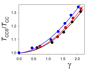
Figure 6: The ratio of the critical cluster concentration temperature at the surface and in the bulk, $T_{CCS}/T_{CC}$, for the same values of $\rho_{0}$. $\gamma$ is the strength of the particle-wall interaction. The symbols denote the simulation results, and the lines are fits to Eq.(6). Black, red and blue lines correspond to $\rho_{0}=0.0005,0.0015,0.005$ respectively. The gas density away from the surface, $\rho_{g}$, depends on $\gamma$. The effect is weak, however, since the increase in $\gamma$ is accompanied by the increase in $T_{CCS}$. The highest change in $\rho_{g}$ is from $\rho_{g}=0.00465$ to $\rho_{g}=0.0049$ along the curve for $\rho_{0}=0.005$.

The simulation results can be fitted quite well to the formula

$$T_{CCS}/T_{CC}=1+B\gamma^{\beta_{0}}.$$ (10)

The fitting parameters for $\rho_{0}=0.0005,0.0015,0.005$ are $B=0.07026,0.07765,0.09833$ and $\beta_{0}=1.938,1.901,1.742$ respectively. The clustering occurs at significantly higher temperature near an adsorbing surface, and the increase of temperature is the larger the stronger the adsorption, and the larger the density in the bulk. One obvious reason for this enhanced clustering is the larger density in the near-surface layer. This layer is a quasi-two dimensional system, and this may influence the aggregation process as well. However, we cannot find an explanation for the power-law behavior with the exponent $\beta_{0}$ decreasing with increasing $\rho_{0}$.

IV.2 the density profile

The density averaged over the plane $(x,y)$ parallel to the wall as a function of the distance from the wall, $z$, should decay in the same way as the pair distribution function. For $g(r)$ given by (LABEL:g(r)), we expect that for large separations,

$$g(z):=\rho(z)/\rho_{g}=1+A\sin(\alpha_{1}z+\phi)e^{-\alpha_{0}z}$$ (11)

where $\alpha_{1}$ and $\alpha_{0}$ should take the same values as in Eq.(5) for $g(r)$ at the same thermodynamic conditions. The remaining parameters depend on $\gamma$. The simulation results and the fit to Eq.(11) are shown in Fig.7 for $z>6$. The agreement is satisfactory.

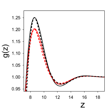
Figure 7: The density profile for $\rho_{0}=0.005$, $T=0.13$. The dotted lines are the simulation results, and the continuous lines are the best fits to Eq.(11). The red and black lines correspond to $\gamma=0.5,1.0$, respectively. The $\alpha_{i}$ parameters in Eq. (11) are taken from the bulk gas simulation. From the fit we obtain $A=17.5,21.5$ and $\phi=0.2$ for $\gamma=0.5,1.0$, respectively. $z$ is in $\sigma$ units.

Much more interesting is the density profile close to the surface. In Fig.8 we present $g(z)$ for different $T$ and $\gamma$. The two maxima corresponding to the first and the second layer of the particles adsorbed at the surface, is followed by a deep and wide minimum that extends up to $z\approx 6$. Note the very small average density for $z\approx 3$. The ratio of the density for $z\approx 3$ and the density in the gas away from the surface decreases significantly with increasing wall-particle attraction, and becomes as small as $10^{-4}$ for $\gamma=1.5$. The essentially empty region rather close to the adsorbing surface results from the formation of a layer consisting of particles that repel each other at distances larger than $r\approx 2$. Accumulated repulsion from the adsorbed particles exceeds the wall-particle attraction for $z\geq 2.5$, and leads to the depletion of the particles beyond the bilayer formed at the surface.

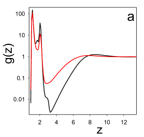
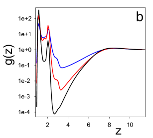
Figure 8: The density profile for $\rho_{0}=0.005$; (a): $\gamma=1$, and $T=0.13,0.17$ for the upper (red) and lower (black) line, respectively, (b): $T=0.13$ and from the bottom to the top lines (black, red, blue) $\gamma=1.5,1,0.5$. $z$ is in $\sigma$ units.

The repulsion from the surface for $2.5\leq z\leq 6$ is stronger when more particles are adsorbed in the two near-surface layers. The strong repulsion barrier prevents from further adsorption of the particles that must overcome this barrier in order to enter the region close enough to the surface, where the attraction dominates (provided that the distance from the adsorbed particles is either smaller than $r\approx 2$ or larger than the range of the repulsion). The formation of the repulsive zone beyond the adsorbed bi- or monolayer of particles, has a significant effect on the dynamics of the adsorption process. Inspired by the Smoluchowski-equation based theory of chemical reactions pedersen:81:0 ; szabo:89:0 , and noting that $g(z)^{-1}$ can be a measure of the repulsive barrier, we introduce the “accessibility time” by

$$\tau_{acc}=\int_{z_{1}}^{z_{2}}g(z)^{-1}dz,$$ (12)

where for the lower and the upper boundary we assume the position of the second maximum of $g(z)$, and $z_{2}=z_{1}+\pi/\alpha_{1}$, respectively, where $\pi/\alpha_{1}$ is half the period of the density wave (see (Eq.(11)). In Fig.9, $1/\tau_{acc}$ is shown for $T=0.13$ as a function of $\gamma$.

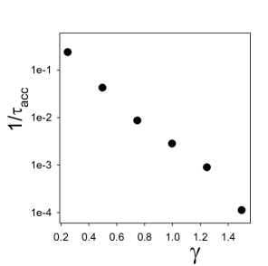
Figure 9: The inverse accessibility time $\tau_{acc}$ defined in Eq.(12) for $T=0.13$ as a function of the strength of the wall-particle attraction.

The plot suggests approximately exponential increase of the accessibility time with $\gamma$. At first sight, it seems counter-intuitive that the stronger the attraction to the surface, the larger time is required to approach it. This paradox is a direct consequence of the competing interactions and formation of the layer of particles that “screen” the attraction to the wall by their repulsive interactions. In MD simulations we indeed see a significant slowing down of the evolution, which makes it difficult to reach the equilibrium state. An anomalous dynamics in the SALR system was recently observed in Ref. zhuang:17:0 ; bergman:19:0 .

IV.3 The adsorption

The adsorption $\Gamma(z_{m})$ (Eq.9), calculated for $z_{m}=1.5,2.6$ is shown in Fig. 10 as a function of $T$ and $\gamma$.

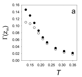
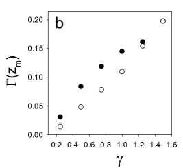
Figure 10: The adsorption (9) for $\rho_{0}=0.005$ and $z_{m}=1.5,2.6$ (open and filled symbols, respectively). (a): as a function of $T$ for $\gamma=1$. (b): as a function of $\gamma$ for $T=0.13$.

For high $T$ or for strong attraction, $\Gamma(1.5)\approx\Gamma(2.6)$, indicating that the particles occupy practically only the first layer. In particular, if $\gamma=1$, the adsorption occurs only in the first layer for $T>0.18\approx T_{CCS}$, i.e. when isolated particles are present near the surface. Below $T_{CCS}$, when clusters appear at the surface, some particles forming the cluster are located in the second layer at $z\approx 2$. This is consistent with the second maximum of $g(z)$ (Fig.8a). On the other hand, the strong attraction to the surface can overcome the particle-particle repulsion, leading to deformation of the clusters. In particular, at $T=0.13$ the clusters become essentially flat for $\gamma>1.2$, consistent with Fig.10b ($\Gamma(1.5)\approx\Gamma(2.6)$) and Fig.8b (the second peak of $g(z)$ is about two orders of magnitude smaller than the first one).

IV.4 structure of the adsorbed layer of particles

A snapshot of the particles adsorbed at the strongly attracting surface with $\gamma=1.5$ for $\rho_{0}=0.005$ and $T=0.13$ is shown in Fig.11. Most of the particles are aggregated into clusters with $M>4$ when attraction to the surface is that strong. Many clusters have a form of a 7-particle “flower” with six particles surrounding the central one, but there exist also larger clusters, with one or two additional particles attached to the flower. Another typical shape is a short piece of a straight bilayer. Irregular shapes appear too. The separation between the neighboring clusters is roughly the same, and locally a hexagonal distribution of the clusters can be observed. The long-range periodic arrangement of the clusters could not be observed, however. The pair distribution function for the centers of mass of the clusters in the $(x,y)$ plane exhibits an oscillatory decay with a large decay length (Fig.12).

In Fig.13 we show a configuration at the surface with stronger wall-particle attraction ($\gamma=2.5$). In this case, stripes of different length form an isotropic labyrinth. In equilibrium we expect stripes too, but it is not clear wheather the isotropic or anisotropic structure with preferred orientation of stripes, found for a similar 2D model in Ref.almarza:14:0 , will occur. Due to the exponentially growing time scale of evolution near the adsorbing surface, it is difficult to reach the equilibrium.

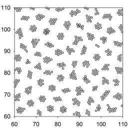
Figure 11: A projection of a representative configuration of the particles adsorbed at the surface for $\rho_{0}=0.005$, $T=0.13$, $\gamma=1.5$ and the adsorption $\Gamma(2.6)\approx 0.2$. The diameter of the shown circles is $r_{min}=1.139$.

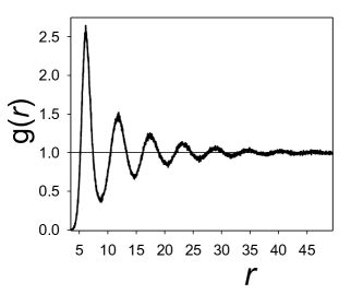
Figure 12: 2D pair distribution function for centers of mass for $M\geq 4$ for $\rho_{0}=0.005$, $T=0.13$ and $\gamma=1.5$. The adsorption for this case is $\Gamma(2.6)\approx 0.2$, and a representative configuration is shown in Fig.11.

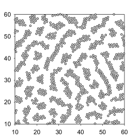
Figure 13: A projection of the representative configuration of the particles adsorbed at the surface for $\rho_{0}=0.00676$, $T=0.15$, $\gamma=2.5$ and the adsorption $\Gamma(2.6)\approx 0.315$. The diameter of the shown circles is $r_{min}=1.139$.

V summary and conclusions

The purpose of our study was determination of general features of adsorption phenomena in dilute systems with particles self-assembling into small clusters. Our MD simulations were performed for a generic model with the SALR potential (1), for various strengths of attraction between the particles and a flat surface.

In the first step we focused on the aggregation in the bulk. We determined the temperature at the critical cluster concentration for three different densities according to the definition of the CCC introduced in Ref.santos:17:0 . At the CCC, the probability of finding a particle in the cluster composed of $M$ particles becomes nonmonotonic. Our histograms and the specific heat (Figs.2 and 5), indicate that one can introduce another structural line determined by the maximum of $c_{V}(T)$. At this line, the probability of finding an isolated particle and a particle inside the cluster of the most probable size are equal. Thus, the maximum of $c_{V}(T)$ represents a crossover from the monomer dominated to the cluster dominated regime in the gas.

We have calculated the pair distribution function $g(r)$. The simulation results fit quite well the simple formula (5) for $r$ larger than the period of the oscillatory decay of $g(r)$.

Near an attractive surface the density of the particles increases, and one can expect an increase of the critical cluster concentration temperature in the near-surface layer. Indeed, we found a significant increase of $T_{CCS}$ with increasing strength of the wall-particle attraction. Simulations indicate that $T_{CCS}(\gamma)/T_{CC}-1\propto\gamma^{\beta_{0}}$ with the exponent $\beta_{0}$ depending on the gas density. Further studies are required to explain the origin of this behavior.

The calculated amount of particles adsorbed in the monolayer and in the bilayer at the surface allows us to follow the scenario of the process of adsorption. When the wall-particle attraction is moderate, and the gas consists of the isolated particles ($T>T_{CCS}$), then the particles are adsorbed in the monolayer at the surface. Below the CCC line, the clusters get adsorbed at the surface, and as they are 3D objects, some part of the cluster occupies the second layer at the surface. However, when $\gamma$ increases, the clusters become flattened, and the excess of density in the second layer decreases. The structure in the first monolayer is shown in Fig.11. We can see that despite the strong wall-particle attraction, a significant fraction of the surface area is not covered by the particles, because they repel each other at large separations.

Perhaps the most interesting result that distinguishes strongly the SALR system from simple fluids, is the formation of a depletion layer just outside the bilayer adsorbed at the surface. The stronger the wall-particle attraction, the smaller the density in the depletion zone. For strong attraction, this depletion layer is essentially empty. This is because the adsorbed bilayer “screens” the attraction of the surface, and the accumulated repulsion from the adsorbed particles forms a large repulsive barrier. We can thus observe an effective repulsion from the attractive surface. The barrier grows in the process of adsorption, and this leads to slowing down of the adsorption - the effect is the stronger, the larger the attraction to the surface.

The effect described above is not specific to the particular model chosen for the simulations, and follows from the presence of the repulsive tail in the interactions. Our results indicate that the adsorption process in a self-assembling system differs significantly from the process in simple fluids. Large strengths of the wall-particle attraction lead to strong effective repulsion beyond the layer adsorbed at the surface. Based on our results, one can expect very nontrivial dynamics of formation of ordered patterns, as has been already observed in Ref. zhuang:17:0 ; bergman:19:0 for the SALR systems in bulk.

It would be interesting to verify our predictions experimentally. An experimental system with the SALR interactions leading to formation of small clusters is for example a much studied dilute solution of lysozyme molecules in deionized water. An attractive surface in this case is for example a weakly charged electrode with an opposite sign, although electrostatic effect may play some role in this case. Another example is provided by weakly charged nanoparticles, with the short-range attraction induced by some kind of small depletion agents present in the solvent, near a surface covered by the same material as the surface of the nanoparticles.

VI Acknowledgements

ML would like to thank prof. Vikhernko for discussions and hospitality during his stay at Belarusian State Technical University. AC is grateful to prof. Zarragoicoechea, Dr. Meyra and Dr. de Virgiliis for discussions, comments on the manuscript and hospitality at the National University of La Plata. This project has received funding from the European Union Horizon 2020 research and innovation programme under the Marie Skłodowska-Curie grant agreement No 734276 (CONIN). An additional support in the years 2017-2018 has been granted for the CONIN project by the Polish Ministry of Science and Higher Education. Financial support from the National Science Center under grant No. 2015/19/B/ST3/03122 is also acknowledged.

References

- (1) A. Imperio and L. Reatto, J. Phys.: Condens. Matter 16, S3769 (2004)
- (2) A. J. Archer and N. B. Wilding, Phys. Rev. E 76, 031501 (2007).
- (3) A. J. Archer, Phys. Rev. E 78, 031402 (2008).
- (4) A. Ciach, Phys. Rev. E 78, 061505 (2008).
- (5) A. Ciach and W. T. Góźdź, Condens. Matter Phys. 13, 23603 (2010).
- (6) P. Kowalczyk, A. Ciach, P. A. Gauden, and A. P. Terzyk, Int. J. Colloid Interface Sci. 363, 579 (2011).
- (7) Y. Zhuang, K. Zhang, and P. Charbonneau, Phys. Rev. Lett. 116, 098301 (2016).
- (8) Y. Zhuang and P. Charbonneau, J. Phys. Chem. B 120, 6178 (2016).
- (9) M. Edelmann and R. Roth, Phys. Rev. E 93, 062146 (2016).
- (10) D. Pini and A. Parola, Soft Matter 13, 9259 (2017).
- (11) A. I. Campbell, V. J.Anderson, J. S. van Duijneveldt, and P. Bartlett, Phys. Rev. Lett. 94, 208301 (2005).
- (12) A. Stradner et al., Nature 432, 492 (2004).
- (13) C. P. Royall, Soft Matter 14, 4020 (2018).
- (14) M. Bergman, T. Garting, P. Schurtenberger, and A. Stradner, J. Phys. Chem. B 123, 2432 (2019).
- (15) A. P. Santos, J. Pȩkalski, and A. Z. Panagiotopoulos, Soft Matter 13, 8055 (2017).
- (16) Y. Hu and P. Charbonneau, Soft Matter 14, 4101 (2018).
- (17) D. Amos, J. Markels, S. Lynn, and C. Radke, J. Phys. Chem. B 102, 2739 (1998).
- (18) M. A. Floriano, E. Caponetti, and A. Z. Panagiotopoulos, Langmuir 15, 3143 (1999).
- (19) N. G. Almarza, J. Pȩkalski, and A. Ciach, J. Chem. Phys. 140, 164708 (2014).
- (20) J. Pȩkalski, A. Ciach, and N. G. Almarza, J. Chem. Phys. 140, 114701 (2014).
- (21) M. Litniewski, J. Phys. Chem. 97, 3842 (1993).
- (22) T. Morishita, J. Chem. Phys. 119, 7075 (2003)
- (23) P. Collins, G. S. Ezra and S. Wiggins, J. Chem. Phys. 133, 014105 (2010)
- (24) M. P. Allen and D. J. Tildesley, Computer Simulations of Liquids (Clarendon Press, Oxford, 1990).
- (25) P. D. Godfrin, N. E. Valadez-Perez, R. Castaneda-Priego, N.J. Wagner and Y. Liu, Soft Mater 10, 5061 (2014)
- (26) J. B. Pedersen and P. Sibani, J. Chem. Phys. 75, 5368 (1981).
- (27) A. Szabo, J.Phys. Chem. 93, 6929 (1989).
- (28) Y. Zhuang and P. Charbonneau, J. Chem. Phys. 147, 091102 (2017).