A Concise Model for Multi-Criteria Chinese Word Segmentation with Transformer Encoder

Abstract

Multi-criteria Chinese word segmentation (MCCWS) aims to exploit the relations among the multiple heterogeneous segmentation criteria and further improve the performance of each single criterion. Previous work usually regards MCCWS as different tasks, which are learned together under the multi-task learning framework. In this paper, we propose a concise but effective unified model for MCCWS, which is fully-shared for all the criteria. By leveraging the powerful ability of the Transformer encoder, the proposed unified model can segment Chinese text according to a unique criterion-token indicating the output criterion. Besides, the proposed unified model can segment both simplified and traditional Chinese and has an excellent transfer capability. Experiments on eight datasets with different criteria show that our model outperforms our single-criterion baseline model and other multi-criteria models. Source codes of this paper are available on Github.

1 Introduction

Chinese word segmentation (CWS) is a preliminary step to process Chinese text. The mainstream CWS methods regard CWS as a character-based sequence labeling problem, in which each character is assigned a label to indicate its boundary information. Recently, various neural models have been explored to reduce efforts of the feature engineering  (Chen et al., 2015a, b; Qun et al., 2020; Wang and Xu, 2017; Kurita et al., 2017; Ma et al., 2018).

Recently, Chen et al. (2017) proposed multi-criteria Chinese word segmentation (MCCWS) to effectively utilize the heterogeneous resources with different segmentation criteria. Specifically, they regard each segmentation criterion as a single task under the framework of multi-task learning, where a shared layer is used to extract the criteria-invariant features, and a private layer is used to extract the criteria-specific features.

However, it is unnecessary to use a specific private layer for each criterion. These different criteria often have partial overlaps. For the example in Table 1, the segmentation of “林丹 (Lin Dan)” is the same in CTB and MSRA criteria, and the segmentation of “总$|$冠军 (the championship)” is the same in PKU and MSRA criteria. All these three criteria have the same segmentation for the word “赢得 (won)”. Although these criteria are inconsistent, they share some partial segmentation. Therefore, it is interesting to use a unified model for all the criteria. At the inference phase, a criterion-token is taken as input to indicate the predict segmentation criterion. Following this idea, Gong et al. (2018) used multiple LSTMs and a criterion switcher at every position to automatically switch the routing among these LSTMs. He et al. (2019) used a shared BiLSTM to deal with all the criteria by adding two artificial tokens at the beginning and end of an input sentence to specify the target criterion. However, due to the long-range dependency problem, BiLSTM is hard to carry the criterion information to each character in a long sentence.

Corpora	Lin	Dan	won	the championship
CTB	林丹		赢得	总冠军
PKU	林	丹	赢得	总	冠军
MSRA	林丹		赢得	总	冠军

Table 1: Illustration of different segmentation criteria.

In this work, we propose a concise unified model for MCCWS task by integrating shared knowledge from multiple segmentation criteria. Inspired by the success of the Transformer Vaswani et al. (2017), we design a fully shared architecture for MCCWS, where a shared Transformer encoder is used to extract the criteria-aware contextual features, and a shared decoder is used to predict the criteria-specific labels. An artificial token is added at the beginning of the input sentence to determine the output criterion. The similar idea is also used in the field of machine translation, Johnson et al. (2017) used a single model to translate between multiple languages. Figure 1 illustrates our model. There are two reasons to use the Transformer encoder for MCCWS. The primary reason is its neatness and ingenious simplicity to model the criterion-aware context representation for each character. Since the Transformer encoder uses self-attention mechanism to capture the interaction each two tokens in a sentence, each character can immediately perceive the information of the criterion-token as well as the context information. The secondary reason is that the Transformer encoder has potential advantages in capturing the long-range context information and having a better parallel efficiency than the popular LSTM-based encoders. Finally, we exploit the eight segmentation criteria on the five simplified Chinese and three traditional Chinese corpora. Experiments show that the proposed model is effective in improving the performance of MCCWS.

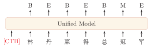
(a) CTB

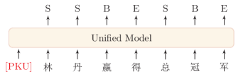
(b) PKU

Figure 1: Unified model for MCCWS. “[$\cdot$]” is a special token indicating the output criterion. The label $\{B,M,E,S\}$ of each character indicates it is the begin, middle, end of a word, or a word with single character.

The contributions of this paper could be summarized as follows.

• We proposed a concise unified model for MCCWS based on Transformer encoder, which adopts a single fully-shared model to segment sentences with a given target criterion. It is attractive in practice to use a single model to produce multiple outputs with different criteria.

• By a thorough investigation, we show the feasibility of using a unified CWS model to segment both simplified and traditional Chinese (see Sec. 4.3). We think it is a promising direction for CWS to exploit the collective knowledge of these two kinds of Chinese.

• The learned criterion embeddings reflect the relations between different criteria, which make our model have better transfer capability to a new criterion (see Sec. 4.4) just by finding a new criterion embedding in the latent semantic space.

• It is a first attempt to train the Transformer encoder from scratch for CWS task. Although we mainly address its conciseness and suitability for MCCWS in this paper and do not intend to optimize a specific Transformer encoder for the single-criterion CWS (SCCWS), we prove that the Transformer encoder is also valid for SCCWS. The potential advantages of the Transformer encoder are that it can effectively extract the long-range interactions among characters and has a better parallel ability than LSTM-based encoders.

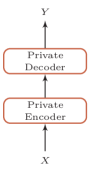
(a) SCCWS

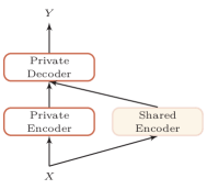
(b) MTL-based MCCWS

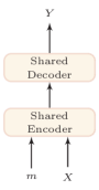
(c) Unified MCCWS

Figure 2: Architectures of SCCWS and MCCWS. The shaded components are shared for different criteria.

2 Background

In this section, we first briefly describe the background knowledge of our work.

2.1 Neural Architecture for CWS

Usually, CWS task could be viewed as a character-based sequence labeling problem. Specifically, each character in a sentence $X=\{x_{1},\dots,x_{T}\}$ is labelled as one of $y\in\mathcal{L}=\{B,M,E,S\}$, indicating the begin, middle, end of a word, or a word with single character. The aim of CWS task is to figure out the ground truth of labels $Y^{*}=\{y_{1}^{*},\dots,y_{T}^{*}\}$:

$$Y^{*}=\operatorname*{arg\,max}_{Y\in\mathcal{L}^{T}}p(Y|X).$$ (1)

Recently, various neural models have been widely used in CWS and can effectively reduce the efforts of feature engineering. The modern architecture of neural CWS usually consists of three components:

Embedding Layer: In neural models, the first step is to map discrete language symbols into distributed embedding space. Formally, each character $x_{t}$ is mapped as $\mathbf{e}_{x_{t}}\in\mathbb{R}^{d_{e}}$, where $d_{e}$ is a hyper-parameter indicating the size of character embedding.

Encoding Layer: The encoding layer is to extract the contextual features for each character.

For example, a prevalent choice for the encoding layer is the bi-directional LSTM (BiLSTM) Hochreiter and Schmidhuber (1997), which could incorporate information from both sides of sequence.

$$\mathbf{h}_{t}=\operatorname*{BiLSTM}(\mathbf{e}_{x_{t}},\overrightarrow{\mathbf{h}}_{t-1},\overleftarrow{\mathbf{h}}_{t+1},\theta_{e}),$$ (2)

where $\overrightarrow{\mathbf{h}}_{t}$ and $\overleftarrow{\mathbf{h}}_{t}$ are the hidden states at step $t$ of the forward and backward LSTMs respectively, $\theta_{e}$ denotes all the parameters in the BiLSTM layer.

Besides BiLSTM, CNN is also alternatively used to extract features.

Decoding Layer: The extracted features are then sent to conditional random fields (CRF) Lafferty et al. (2001) layer or multi-layer perceptron (MLP) for tag inference.

When using CRF as decoding layer, $p(Y|X)$ in Eq (1) could be formalized as:

$$p(Y|X)=\frac{\Psi(Y|X)}{\sum_{Y^{\prime}\in\mathcal{L}^{n}}\Psi(Y^{\prime}|X)},$$ (3)

where $\Psi(Y|X)$ is the potential function. In first order linear chain CRF, we have:

$$\Psi(Y|X)=\prod_{t=2}^{n}\psi(X,t,y_{t-1},y_{t}),$$ (4)

$$\psi(\mathbf{x},t,y^{\prime},y)=\exp(\delta(X,t)_{y}+\mathbf{b}_{y^{\prime}y}),$$ (5)

where $\mathbf{b}_{y^{\prime}y}\in\mathbf{R}$ is trainable parameters respective to label pair $(y^{\prime},y)$, score function $\delta(X,t)\in\mathbb{R}^{|\mathcal{L}|}$ calculates scores of each label for tagging the $t$-th character:

$$\delta(X,t)=\mathbf{W}_{\delta}^{\top}\mathbf{h}_{t}+\mathbf{b}_{\delta},$$ (6)

where $\mathbf{h}_{t}$ is the hidden state of encoder at step $t$, $\mathbf{W}_{\delta}\in\mathbb{R}^{d_{h}\times|\mathcal{L}|}$ and $\mathbf{b}_{\delta}\in\mathbb{R}^{|\mathcal{L}|}$ are trainable parameters.

When using MLP as decoding layer, $p(Y|X)$ in Eq (1) is directly predicted by a MLP with softmax function as output layer.

$$p(y_{t}|X)=\mathrm{MLP}(\mathbf{h}_{t},\theta_{d}),\qquad\forall t\in[1,T]$$ (7)

where $\theta_{d}$ denotes all the parameters in MLP layer.

Most current state-of-the-art CWS models Chen et al. (2015a); Xu and Sun (2016); Liu et al. (2016); Yang et al. (2018); Qun et al. (2020) mainly focus on single-criterion CWS (SCCWS). Figure 2a shows the architecture of SCCWS.

2.2 MCCWS with Multi-Task Learning

To improve the performance of CWS by exploiting multiple heterogeneous criteria corpora, Chen et al. (2017) utilize the multi-task learning framework to model the shared information among these different criteria.

Formally, assuming that there are $M$ corpora with heterogeneous segmentation criteria, we refer $\mathcal{D}_{m}$ as corpus $m$ with $N_{m}$ samples:

$$\mathcal{D}_{m}=\{(X_{n}^{(m)},Y_{n}^{(m)})\}_{n=1}^{N_{m}},$$ (8)

where $X_{n}^{(m)}$ and $Y_{n}^{(m)}$ denote the $n$-th sentence and the corresponding label in corpus $m$ respectively.

The encoding layer introduces a shared encoder to mine the common knowledge across multiple corpora, together with the original private encoder. The architecture of MTL-based MCCWS is shown in Figure 2b.

Concretely, for corpus $m$, a shared encoder and a private encoder are first used to extract the criterion-agnostic and criterion-specific features.

$$\mathbf{H}^{(s)}= \mathbf{enc}_{s}(\mathbf{e}_{X};\theta^{(s)}_{e}),$$ (9)

$$\mathbf{H}^{(m)}= \mathbf{enc}_{m}(\mathbf{e}_{X};\theta^{(m)}_{e}),\quad\forall m\in[1,M]$$ (10)

where $\mathbf{e}_{X}=\{\mathbf{e}_{x_{1}},\cdots,\mathbf{e}_{x_{T}}\}$ denotes the embeddings of the input characters $x_{1},\cdots,x_{T}$, $\mathbf{enc}_{s}(\cdot)$ represents the shared encoder and $\mathbf{enc}_{m}(\cdot)$ represents the private encoder for corpus $m$; $\theta^{(s)}_{e}$ and $\theta^{(m)}_{e}$ are the shared and private parameters respectively. The shared and private encoders are usually implemented by the RNN or CNN network.

Then a private decoder is used to predict criterion-specific labels. For the $m$-th corpus, the probability of output labels is

$$p_{m}(Y|X) =\mathbf{dec}_{m}([\mathbf{H}^{(s)};\mathbf{H}^{(m)}];\theta^{(m)}_{d}),$$ (11)

where $\mathbf{dec}_{m}(\cdot)$ is a private CRF or MLP decoder for corpus $m(m\in[1,M])$, taking the shared and private features as inputs; $\theta^{(m)}_{d}$ is the parameters of the $m$-th private decoder.

Objective

The objective is to maximize the log likelihood of true labels on all the corpora:

$$\mathcal{J}_{seg}(\Theta^{m},\Theta^{s})=\sum_{m=1}^{M}\sum_{n=1}^{N_{m}}\log p_{m}(Y^{(m)}_{n}|X^{(m)}_{n};\Theta^{m},\Theta^{s}),$$ (12)

where $\Theta^{m}$ = $\{\theta^{(m)}_{e},\theta^{(m)}_{d}\}$ and $\Theta^{s}$ = $\{\mathbf{E},\theta^{(s)}_{e}\}$ denote all the private and shared parameters respectively; $\mathbf{E}$ is the embedding matrix.

3 Proposed Unified Model

In this work, we propose a more concise architecture for MCCWS, which adopts the Transformer encoder Vaswani et al. (2017) to extract the contextual features for each input character. In our proposed architecture, both the encoder and decoder are shared by all the criteria. The only difference for each criterion is that a unique token is taken as input to specify the target criterion, which makes the shared encoder to capture the criterion-aware representation. Figure 2 illustrates the difference between our proposed model and the previous models. A more detailed architecture for MCCWS is shown in Figure 3.

3.1 Embedding Layer

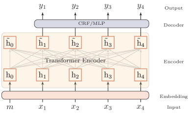
Figure 3: Proposed Model for MCCWS.

Given a sentence $X=\{x_{1},\dots,x_{T}\}$, we first map it into a vector sequence where each token is a $d_{model}$ dimensional vector. Besides the standard character embedding, we introduce three extra embeddings: criterion embedding, bigram embedding, and position embedding.

1) Criterion Embedding: Firstly, we add a unique criterion-token at the beginning of $X$ to indicate the output criterion. For the $m$-th criterion, the criterion-token is $[m]$. We use $\mathbf{e}_{[m]}$ to denote its embedding. Thus, the model can learn the relations between different criteria in the latent embedding space.

2) Bigram Embedding: Based on Chen et al. (2015b); Shao et al. (2017); Zhang et al. (2018), the character-level bigram features can significantly benefit the task of CWS. Following their settings, we also introduce the bigram embedding to augment the character-level unigram embedding. The representation of character $x_{t}$ is

$$\mathbf{e}^{\prime}_{x_{t}}=FC(\mathbf{e}_{x_{t}}\oplus\mathbf{e}_{x_{t-1}x_{t}}\oplus\mathbf{e}_{x_{t}x_{t+1}}),$$ (13)

where $\mathbf{e}$ denotes the $d$-dimensional embedding vector for the unigram and bigram, $\oplus$ is the concatenation operator, and FC is a fully connected layer to map the concatenated character embedding with the dimension $3d$ into the embedding $\mathbf{e}^{\prime}_{x_{t}}\in\mathbb{R}^{d_{model}}$.

3) Position Embedding: To capture the order information of a sequence, a position embedding $PE$ is used for each position. The position embedding can be learnable parameters or predefined. In this work, we use the predefined position embedding following Vaswani et al. (2017). For the $t$-th character in a sentence, its position embedding is defined by

$$PE_{t,2i}= \sin(t/10000^{2i/d_{model}}),$$ (14)

$$PE_{t,2i+1}= \cos(t/10000^{2i/d_{model}}),$$ (15)

where $i$ denotes the dimensional index of position embedding.

Finally, the embedding matrix of the sequence $X=\{x_{1},\cdots,x_{T}\}$ with criterion $m$ is formulated as

$$\mathbf{H} =[\mathbf{e}_{[m]}+PE_{0};\mathbf{e}^{\prime}_{x_{1}}+PE_{1};\cdots;\mathbf{e}^{\prime}_{x_{T}}+PE_{T}],$$ (16)

where $\mathbf{H}\in\mathbb{R}^{(T+1)\times d_{model}}$, $(T+1)$ and $d_{model}$ represent the length and the dimension of the input vector sequence.

3.2 Encoding Layer

In sequence modeling, RNN and CNN often suffer from the long-term dependency problem and cannot effectively extract the non-local interactions in a sentence. Recently, the fully-connected self-attention architecture, such as Transformer Vaswani et al. (2017), achieves great success in many NLP tasks.

In this work, we adopt the Transformer encoder as our encoding layer, in which several multi-head self-attention layers are used to extract the contextual feature for each character.

Given a sequence of vectors $H\in\mathbb{R}^{(T+1)\times d_{model}}$, a single-head self-attention projects $H$ into three different matrices: the query matrix $Q\in\mathbb{R}^{(T+1)\times d_{k}}$, the key matrix $K\in\mathbb{R}^{(T+1)\times d_{k}}$ and the value matrix $V\in\mathbb{R}^{(T+1)\times d_{v}}$, and uses scaled dot-product attention to get the output representation.

$$Q,K,V=HW^{Q},HW^{K},HW^{V}$$ (17)

$$\mathrm{Attn}(Q,K,V)=\mathrm{softmax}(\frac{QK^{T}}{\sqrt{d_{k}}})V,$$ (18)

where the matrices $W^{Q}\in\mathbb{R}^{d_{model}\times d_{k}},W^{K}\in\mathbb{R}^{d_{model}\times d_{k}},W^{V}\in\mathbb{R}^{d_{model}\times d_{v}}$ are learnable parameters and $\mathrm{softmax}(\cdot)$ is performed row-wise.

The Transformer encoder consists of several stacked multi-head self-attention layers and fully-connected layers. Assuming the input of the multi-head self-attention layer is $H$, its output $\tilde{H}$ is calculated by

$$Z= \textrm{layer-norm}\Big{(}H+\mathrm{MultiHead}(H)\Big{)},$$ (19)

$$\tilde{H}= \textrm{layer-norm}\Big{(}Z+\mathrm{FFN}(Z)\Big{)},$$ (20)

where $\textrm{layer-norm}(\cdot)$ represents the layer normalization Ba et al. (2016) .

All the tasks with the different criteria use the same encoder. Nevertheless, with the different criterion-token $[m]$, the encoder can effectively extract the criterion-aware representation for each character.

3.3 Decoding Layer

In the standard multi-task learning framework, each task has its private decoder to predict the task-specific labels. Different from the previous work, we use a shared decoder for all the tasks since we have extracted the criterion-aware representation for each character. In this work, we use CRF as the decoder since it is slightly better than MLP (see Sec. 4.2).

With the fully-shared encoder and decoder, our model is more concise than the shared-private architectures Chen et al. (2017); Huang et al. (2019).

4 Experiments

Table 2: Details of the eight datasets after preprocessing. “Word Types” represents the number of unique word. “Char Types” is the number of unique characters. “OOV Rate” is Out-Of-Vobulary rate.

Corpora			Words#	Chars#	Word Types	Char Types	OOV
Sighan05	MSRA	Train	2.4M	4.0M	75.4K	5.1K
		Test	0.1M	0.2M	11.9K	2.8K	1.32%
	AS	Train	5.4M	8.3M	128.8K	5.8K
		Test	0.1M	0.2M	18.0K	3.4K	2.20%
	PKU	Train	1.1M	1.8M	51.2K	4.6K
		Test	0.1M	0.2M	12.5K	2.9K	2.06%
	CITYU	Train	1.1M	1.8M	43.4K	4.2K
		Test	0.2M	0.4M	23.2K	3.6K	3.69%
Sighan08	CTB	Train	0.6M	1.0M	40.5K	4.2K
		Test	0.1M	0.1M	11.9K	2.9K	3.80%
	CKIP	Train	0.7M	1.1M	44.7K	4.5K
		Test	0.1M	0.1M	14.2K	3.1K	4.29%
	NCC	Train	0.9M	1.4M	53.3K	5.3K
		Test	0.2M	0.2M	20.9K	3.9K	3.31%
	SXU	Train	0.5M	0.8M	29.8K	4.1K
		Test	0.1M	0.2M	11.6K	2.8K	2.60%

Datasets We use eight CWS datasets from SIGHAN2005 Emerson (2005) and SIGHAN2008 Jin and Chen (2008). Among them, the AS, CITYU, and CKIP datasets are in traditional Chinese, while the MSRA, PKU, CTB, NCC, and SXU datasets are in simplified Chinese. Except where otherwise stated, we follow the setting of Chen et al. (2017); Gong et al. (2018), and translate the AS, CITYU and CKIP datasets into simplified Chinese. We do not balance the datasets and randomly pick 10% examples from the training set as the development set for all datasets. Similar to the previous work Chen et al. (2017), we preprocess all the datasets by replacing the continuous Latin characters and digits with a unique token, and converting all digits, punctuation and Latin letters to half-width to deal with the full/half-width mismatch between training and test set.

We have checked the annotation schemes of different datasets, which are just partially shared and no two datasets have the same scheme. According to our statistic, the averaged overlap is about 20.5% for 3-gram and 4.4% for 5-gram.

Table 2 gives the details of the eight datasets after preprocessing. For training and development sets, lines are split into shorter sentences or clauses by punctuations, in order to make a faster batch.

Pre-trained Embedding Based on on Chen et al. (2015b); Shao et al. (2017); Zhang et al. (2018), n-gram features are of great benefit to Chinese word segmentation and POS tagging tasks. Thus we use unigram and bigram embeddings for our models. We first pre-train unigram and bigram embeddings on Chinese Wikipedia corpus by the method proposed in Ling et al. (2015), which improves standard word2vec by incorporating token order information.

Embedding Size $d$	100
Hidden State Size $d_{model}$	256
Transformer Encoder Layers	6
Attention Heads	4
Batch Size	256
Dropout Ratio	0.2
Warmup Steps	4000

Table 3: Hyper-Parameter Settings

Hyper-parameters We use Adam optimizer Kingma and Ba (2014) with the same warmup strategy as Vaswani et al. (2017). The development set is used for parameter tuning. All the models are trained for 100 epochs. Pre-trained embeddings are fixed for the first 80 epochs and then updated during the following epochs. After each training epoch, we test the model on the dev set, and models with the highest $F1$ in the dev set are used in the test set. Table 3 shows the detailed hyperparameters.

Models		MSRA	AS	PKU	CTB	CKIP	CITYU	NCC	SXU	Avg.
Single-Criterion Models
Stacked BiLSTM Ma et al. (2018)	F	97.4	96.2	96.1	96.7	-	97.2	-	-	-
BiLSTM Chen et al. (2017)	F	95.84	94.2	93.3	95.3	93.06	94.07	92.17	95.17	94.14
Switch-LSTMs Gong et al. (2018)	F	96.46	94.51	95.74	97.09	92.88	93.71	92.12	95.57	94.76
Transformer Encoder	F	98.07	96.06	96.39	96.41	95.66	96.32	95.57	97.08	96.45
Transformer Encoder	OOV	73.75	73.05	72.82	82.82	79.05	83.72	71.81	77.95	76.87
Multi-Criteria Models
BiLSTM Chen et al. (2017)	F	96.04	94.64	94.32	96.18	94.26	95.55	92.83	96.04	94.98
Switch-LSTMs Gong et al. (2018)	F	97.78	95.22	96.15	97.26	94.99	96.22	94.12	97.25	96.12
Unified BiLSTM He et al. (2019)	F	97.2	95.4	96.0	96.7	-	96.1	-	96.4	-
Our Unified Model	F	98.05	96.44	96.41	96.99	96.51	96.91	96.04	97.61	96.87
Our Unified Model	OOV	78.92	76.39	78.91	87	82.89	86.91	79.3	85.08	81.92

Table 4: Overall results on eight CWS datasets. F and OOV indicate the $F1$ score and OOV recall, respectively. The upper block consists of single-criterion models. Since Stacked BiLSTM Ma et al. (2018) is a strong SOTA model, the other comparable CWS models are omitted for brevity. The lower block consists of multi-criteria models.

Models	MSRA	AS	PKU	CTB	CKIP	CITYU	NCC	SXU	Avg.
Unified Model	98.05	96.44	96.41	96.99	96.51	96.91	96.04	97.61	96.87
w/o CRF	98.02	96.42	96.41	96.9	96.59	96.87	95.96	97.5	96.83
w/o bigram	97.41	96	96.25	96.71	96	96.31	94.62	96.84	96.27
w/o pre-trained emb.	97.51	96.06	96.02	96.47	96.22	95.99	94.82	96.76	96.23

Table 5: Ablation experiments.

4.1 Overall Results

Table 4 shows the experiment results of the proposed model on test sets of eight CWS datasets.

We first compare our Transformer encoder with the previous models in the single-criterion scenario. The comparison is presented in the upper block of Table 4. Since Switch-LSTMs Gong et al. (2018) is designed form MCCWS, it is just slight better than BiLSTM in single-criterion scenario. Compared to the LSTM-based encoders, the Transformer encoder brings a noticeable improvement compared to Chen et al. (2017); Gong et al. (2018), and gives a comparable performance to Ma et al. (2018). In this work, we do not intend to prove the superiority of the Transformer encoder over LSTM-based encoders in the single-criterion scenario. Our purpose is to build a concise unified model based on Transformer encoder for MCCWS.

In the multi-criteria scenario, we compare our unified model with the BiLSTM Chen et al. (2017) and Switch-LSTMs Gong et al. (2018). The lower block of Table 4 displays the contrast. Firstly, although different criteria are trained together, our unified model achieves better performance besides CTB. Compared to the single-criterion scenario, 0.42 gain in average $F1$ score is obtained by the multi-criteria scenario. Moreover, our unified model brings a significant improvement of 5.05 in OOV recall. Secondly, compared to previous MCCWS models, our unified model also achieves better average $F1$ score. Especially, our unified model significantly outperforms the unified BiLSTM He et al. (2019), which indicates the Transformer encoder is more effective in carrying the criterion information than BiLSTM. The reason is that the Transformer encoder can model the interaction of the criterion-token and each character directly, while BiLSTM needs to carry the criterion information step-by-step from the two ends to the middle of the input sentence. The criterion information could be lost for the long sentences.

There are about 200 sentences are shared by more than one datasets with different segmentation schemes, but it is not much harder to correctly segment them. Their F1 score is 96.84.

Models	MSRA	AS	PKU	CTB	CKIP	CITYU	NCC	SXU	Avg. F1
8Simp	98.05	96.44	96.41	96.99	96.51	96.91	96.04	97.61	96.87
8Trad	97.98	96.39	96.49	96.99	96.49	96.86	95.98	97.48	96.83
5Simp, 3Trad	98.03	96.52	96.6	96.94	96.38	96.8	96.02	97.55	96.86
8 Simp, 8 Trad	98.04	96.41	96.43	96.99	96.54	96.85	96.08	97.52	96.86

Table 6: Joint training on both the simplified and traditional Chinese corpus.

Figure 4 visualizes the 2D PCA projection of the learned embeddings of eight different criteria. Generally, the eight criteria are mapped into dispersed points in the embedding space, which indicates that each criterion is different from others. Among them, MSRA is obviously different from others. A possible reason is that the named entity is regarded as a whole word in the MSRA criterion, which is significantly distinguishing with other criteria.

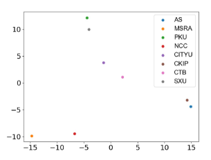
Figure 4: Visualization of the criterion embeddings.

4.2 Ablation Study

Table 5 shows the effectiveness of each component in our model.

苹果 (apple)	蘋果 (apple)	爱好(hobby)	愛好(hobby)	担心(worry)	擔心(worry)
坚果(nut)	微軟(Microsoft)	热爱(love)	熱愛(love)	关心(care)	關心(care)
谷歌(Google)	黃油 (butter)	兴趣(interest)	爱好(hobby)	怀疑(doubt)	顧慮(misgiving)
华为(Huawei)	現貨(goods in stock)	愛好(hobby)	興趣(interest)	顾虑(misgiving)	懷疑(doubt)
黄油(butter)	果凍(jelly)	梦想(dream)	夢想(dream)	担忧(concern)	擔憂(concern)
鲜果(fresh fruit)	京東(JD)	爱玩(Playful)	愛玩(playful)	责怪(blame)	憂慮(anxiety)
微软(Microsoft)	賣家(seller)	痴迷(addict)	喜愛(adore)	伤心(sad)	責怪(blame)
诺基(Nokia)	苹果(apple)	乐趣 (pleasure)	習慣(habbit)	嫌弃(disfavour)	傷心(sad)
蘋果(Apple)	售後(after-sales)	喜爱 (adore)	樂趣(pleasure)	忧虑(anxiety)	担心(worry)

Table 7: Qualitative analysis for the joint embedding space of simplified and traditional Chinese. Given the target bigram, we list its top 8 similar bigrams. The bigram with red color indicates it is traditional Chinese.

The first ablation study is to verify the effectiveness of the CRF decoder, which is popular in most CWS models. The comparison between the first two lines indicates that with or without CRF does not make much difference. Since a model with CRF takes a longer time to train and inference, we suggest not to use CRF in Transformer encoder models in practice.

The other two ablation studies are to evaluate the effect of the bigram feature and pre-trained embeddings. We can see that their effects vary in different datasets. Some datasets are more sensitive to the bigram feature, while others are more sensitive to pre-trained embeddings. In terms of average performance, the bigram feature and pre-trained embeddings are important and boost the performance considerably, but these two components do not have a clear winner.

4.3 Joint Training on both simplified and Traditional Corpora

In the above experiments, the traditional Chinese corpora (AS, CITYU, and CKIP) are translated into simplified Chinese. However, it might be more attractive to jointly train a unified model directly on the mixed corpora of simplified and traditional Chinese without translation. As a reference, the single model has been used to translate between multiple languages in the field of machine translation Johnson et al. (2017).

To thoroughly investigate the feasibility of this idea, we study four different settings to train our model on simplified and traditional Chinese corpora.

1. The first setting (“8Simp”) is to translate all the corpora into simplified Chinese. For the pre-trained embeddings, we use the simplified Chinese Wikipedia dump to pre-train the unigram and bigram embeddings. This way is the same as the previous experiments.

2. The second setting (“8Trad”) is to translate all the corpora into traditional Chinese. For the pre-trained embeddings, we first convert the Wikipedia dump into traditional Chinese characters, then we use this converted corpus to pre-train unigram and bigram embeddings.

3. The third setting (“5Simp, 3Trad”) is to keep the original characters for five simplified Chinese corpora and three traditional Chinese corpora without translation. The unified model can take as input the simplified or traditional Chinese sentences. In this way, we pre-train the joint simplified and traditional Chinese embeddings in a joint embedding space. We merge the Wikipedia corpora used in “8Trad” and “8Simp” to form a mixed corpus, which contains both the simplified and traditional Chinese characters. The unigram and bigram embeddings are pre-trained on this mixed corpus.

4. The last setting (“8Simp, 8Trad”) is to simultaneously train our model on both the eight simplified Chinese corpora in “8Simp” and the eight traditional Chinese corpora in “8Trad”. The pre-trained word embeddings are the same as “5Simp, 3Trad”.

Table 6 shows that there does not exist too much difference between different settings. This investigation indicates it is feasible to train a unified model directly on two kinds of Chinese characters.

To better understand the quality of the learned joint embedding space of the simplified and traditional Chinese, we conduct a qualitative analysis to illustrate the most similar bigrams for a target bigram. Similar bigrams are retrieved based on the cosine similarity calculated using the learned embeddings. As shown in Table 7, the traditional Chinese bigrams are similar to their simplified Chinese counterparts, and vice versa. The results show that the simplified and traditional Chinese bigrams are aligned well in the joint embedding space.

4.4 Transfer Capability

Since except for the criterion embedding, the other parts of the unified model are the same for different criteria, we want to exploit whether a trained unified model can be transferred to a new criterion only by learning a new criterion embedding with few examples.

Figure 5: Evaluation of the transfer capability. Switch-LSTMs and Ours are models trained on the given instances from scratch. Switch-LSTMs^(trans) and Ours^(trans) are models learned in transfer fashion.

We use the leave-one-out strategy to evaluate the transfer capability of our unified model. We first train a model on seven datasets, then only learn the new criterion embedding with a few training instances from the left dataset. This scenario is also discussed in Gong et al. (2018), and Figure 5 presents their and our outcomes (averaged $F1$ score). There are two observations: Firstly, for the different number of samples, the transferred model always largely outperforms the models learned from scratch. We believe this indicates that learning a new criterion embedding is an effective way to transfer a trained unified model to a new criterion. Secondly, our model also has superior transferability than Switch-LSTMs (Ours^(trans) versus Switch-LSTMs^(trans)).

5 Related Work

The previous work on the MCCWS can be categorized into two lines.

One line is multi-task based MCCWS. Chen et al. (2017) proposed a multi-criteria learning framework for CWS, which uses a shared layer to extract the common underlying features and a private layer for each criterion to extract criteria-specific features. Huang et al. (2019) proposed a domain adaptive segmenter to capture diverse criteria based on Bidirectional Encoder Representations from Transformer (BERT) Devlin et al. (2018).

Another line is unified MCCWS. Gong et al. (2018) presented Switch-LSTMs to segment sentences, which consists of several LSTM layers, and uses a criterion switcher at every position to change the routing among these LSTMs automatically. However, the complexity of the model makes Switch-LSTMs hard to be applied in practice. He et al. (2019) used a shared BiLSTM by adding two artificial tokens at the beginning and end of an input sentence to specify the output criterion. However, due to the long-range dependency problem, BiLSTM is hard to carry the criterion information to each character in a long sentence.

Compared to the above two unified models, we use the Transformer encoder in our unified model, which can elegantly model the criterion-aware context representation for each character. With the Transformer, we just need a special criterion-token to specify the output criterion. Each character can directly attend the criterion-token to be aware of the target criterion. Thus, we can use a single model to produce different segmented results for different criteria. Different from Huang et al. (2019), which uses the pre-trained Transformer BERT and several extra projection layers for different criteria, our model is a fully-shared and more concise.

6 Conclusion and Future Work

We propose a concise unified model for MCCWS, which uses the Transformer encoder to extract the criterion-aware representation according to a unique criterion-token. Experiments on eight corpora show that our proposed model outperforms the previous models and has a stronger transfer capability. The conciseness of our model makes it easy to be applied in practice.

In this work, we only adopt the vanilla Transformer encoder since we just want to utilize its self-attention mechanism to model the criterion-aware context representation for each character neatly. Therefore, it is promising for future work to look for the more effective adapted Transformer encoder for CWS task or to utilize the pre-trained models Qiu et al. (2020), such as BERT-based MCCWS Ke et al. (2020). Besides, we are also planning to incorporate other sequence labeling tasks into the unified model, such as POS tagging and named entity recognition.

7 Acknowledgements

This work was supported by the National Natural Science Foundation of China (No. 62022027 and 61976056), Science and Technology on Parallel and Distributed Processing Laboratory (PDL).

References

- Ba et al. (2016) Lei Jimmy Ba, Ryan Kiros, and Geoffrey E. Hinton. 2016. Layer normalization. CoRR, abs/1607.06450.
- Chen et al. (2015a) Xinchi Chen, Xipeng Qiu, Chenxi Zhu, and Xuanjing Huang. 2015a. Gated recursive neural network for Chinese word segmentation. In Proceedings of Annual Meeting of the Association for Computational Linguistics.
- Chen et al. (2015b) Xinchi Chen, Xipeng Qiu, Chenxi Zhu, Pengfei Liu, and Xuanjing Huang. 2015b. Long Short-Term Memory Neural Networks for Chinese Word Segmentation. In EMNLP, pages 1197–1206.
- Chen et al. (2017) Xinchi Chen, Zhan Shi, Xipeng Qiu, and Xuanjing Huang. 2017. Adversarial multi-criteria learning for Chinese word segmentation. In Proceedings of the 55th Annual Meeting of the Association for Computational Linguistics (Volume 1: Long Papers), volume 1, pages 1193–1203.
- Devlin et al. (2018) Jacob Devlin, Ming-Wei Chang, Kenton Lee, and Kristina Toutanova. 2018. BERT: pre-training of deep bidirectional transformers for language understanding. CoRR, abs/1810.04805.
- Emerson (2005) T. Emerson. 2005. The second international Chinese word segmentation bakeoff. In Proceedings of the Fourth SIGHAN Workshop on Chinese Language Processing, pages 123–133. Jeju Island, Korea.
- Gong et al. (2018) Jingjing Gong, Xinchi Chen, Tao Gui, and Xipeng Qiu. 2018. Switch-LSTMs for multi-criteria chinese word segmentation. arXiv preprint arXiv:1812.08033.
- He et al. (2019) Han He, Lei Wu, Hua Yan, Zhimin Gao, Yi Feng, and George Townsend. 2019. Effective neural solution for multi-criteria word segmentation. In Smart Intelligent Computing and Applications, pages 133–142. Springer.
- Hochreiter and Schmidhuber (1997) Sepp Hochreiter and Jürgen Schmidhuber. 1997. Long short-term memory. Neural computation, 9(8):1735–1780.
- Huang et al. (2019) Weipeng Huang, Xingyi Cheng, Kunlong Chen, Taifeng Wang, and Wei Chu. 2019. Toward fast and accurate neural chinese word segmentation with multi-criteria learning. arXiv preprint arXiv:1903.04190.
- Jin and Chen (2008) G. Jin and X. Chen. 2008. The fourth international chinese language processing bakeoff: Chinese word segmentation, named entity recognition and chinese pos tagging. In Sixth SIGHAN Workshop on Chinese Language Processing, page 69.
- Johnson et al. (2017) Melvin Johnson, Mike Schuster, Quoc V Le, Maxim Krikun, Yonghui Wu, Zhifeng Chen, Nikhil Thorat, Fernanda Viégas, Martin Wattenberg, Greg Corrado, et al. 2017. Google’s multilingual neural machine translation system: Enabling zero-shot translation. Transactions of the Association for Computational Linguistics, 5:339–351.
- Ke et al. (2020) Zhen Ke, Liang Shi, Erli Meng, Bin Wang, Xipeng Qiu, and Xuanjing Huang. 2020. Unified multi-criteria chinese word segmentation with bert. arXiv preprint arXiv:2004.05808.
- Kingma and Ba (2014) Diederik Kingma and Jimmy Ba. 2014. Adam: A method for stochastic optimization. arXiv preprint arXiv:1412.6980.
- Kurita et al. (2017) Shuhei Kurita, Daisuke Kawahara, and Sadao Kurohashi. 2017. Neural joint model for transition-based Chinese syntactic analysis. In Proceedings of the 55th Annual Meeting of the Association for Computational Linguistics, volume 1, pages 1204–1214.
- Lafferty et al. (2001) John D. Lafferty, Andrew McCallum, and Fernando C. N. Pereira. 2001. Conditional random fields: Probabilistic models for segmenting and labeling sequence data. In Proceedings of the Eighteenth International Conference on Machine Learning.
- Ling et al. (2015) Wang Ling, Chris Dyer, Alan W Black, and Isabel Trancoso. 2015. Two/too simple adaptations of word2vec for syntax problems. In Proceedings of the 2015 Conference of the North American Chapter of the Association for Computational Linguistics: Human Language Technologies, pages 1299–1304.
- Liu et al. (2016) Yijia Liu, Wanxiang Che, Jiang Guo, Bing Qin, and Ting Liu. 2016. Exploring segment representations for neural segmentation models. arXiv preprint arXiv:1604.05499.
- Ma et al. (2018) Ji Ma, Kuzman Ganchev, and David Weiss. 2018. State-of-the-art Chinese word segmentation with Bi-LSTMs. arXiv preprint arXiv:1808.06511.
- Qiu et al. (2020) Xipeng Qiu, Tianxiang Sun, Yige Xu, Yunfan Shao, Ning Dai, and Xuanjing Huang. 2020. Pre-trained models for natural language processing: A survey. SCIENCE CHINA Technological Sciences.
- Qun et al. (2020) Nuo Qun, Hang Yan, Xipeng Qiu, and Xuanjing Huang. 2020. Chinese word segmentation via BiLSTM+Semi-CRF with relay node. Journal of Computer Science and Technology, 35(5):1115–1126.
- Shao et al. (2017) Yan Shao, Christian Hardmeier, Jörg Tiedemann, and Joakim Nivre. 2017. Character-based joint segmentation and pos tagging for chinese using bidirectional rnn-crf. arXiv preprint arXiv:1704.01314.
- Vaswani et al. (2017) Ashish Vaswani, Noam Shazeer, Niki Parmar, Jakob Uszkoreit, Llion Jones, Aidan N Gomez, Łukasz Kaiser, and Illia Polosukhin. 2017. Attention is all you need. In Advances in Neural Information Processing Systems, pages 5998–6008.
- Wang and Xu (2017) Chunqi Wang and Bo Xu. 2017. Convolutional neural network with word embeddings for Chinese word segmentation. arXiv preprint arXiv:1711.04411.
- Xu and Sun (2016) Jingjing Xu and Xu Sun. 2016. Dependency-based gated recursive neural network for chinese word segmentation. In Proceedings of the 54th Annual Meeting of the Association for Computational Linguistics (Volume 2: Short Papers), pages 567–572.
- Yang et al. (2018) Jie Yang, Yue Zhang, and Shuailong Liang. 2018. Subword encoding in lattice LSTM for Chinese word segmentation. arXiv preprint arXiv:1810.12594.
- Zhang et al. (2018) Meishan Zhang, Nan Yu, and Guohong Fu. 2018. A simple and effective neural model for joint word segmentation and POS tagging. IEEE/ACM Transactions on Audio, Speech and Language Processing (TASLP), 26(9):1528–1538.