Evaluation of Abramowitz functions in the right half of the complex plane

Abstract

A numerical scheme is developed for the evaluation of Abramowitz functions $J_{n}$ in the right half of the complex plane. For $n=-1,\,\ldots,\,2$, the scheme utilizes series expansions for $|z|<1$ and asymptotic expansions for $|z|>R$ with $R$ determined by the required precision, and modified Laurent series expansions which are precomputed via a least squares procedure to approximate $J_{n}$ accurately and efficiently on each sub-region in the intermediate region $1\leq|z|\leq R$. For $n>2$, $J_{n}$ is evaluated via a recurrence relation. The scheme achieves nearly machine precision for $n=-1,\ldots,2$, with the cost about four times of evaluating a complex exponential per function evaluation.

1 Introduction

The Abramowitz functions $J_{n}$ of order $n$, defined by

$$J_{n}(z)=\int_{0}^{\infty}t^{n}e^{-t^{2}-z/t}dt,\quad n\in\mathbb{Z},$$ (1)

are frequently encountered in kinetic theory (cf., e.g., [7, 14]), where the integral equations resulting from linearization of the Boltzmann equation have these functions (cf., e.g., [7, 14, 19, 16]) as the kernels. The $n$-th order Abramowitz function $J_{n}$ satisfies the third order ODE [1, 2]

$$zJ_{n}^{{}^{\prime\prime\prime}}-(n-1)J_{n}^{{}^{\prime\prime}}+2J_{n}=0$$ (2)

and the recurrence relations

$$J_{n}^{\prime}(z)=-J_{n-1}(z),$$ (3)

$$2J_{n}(z)=(n-1)J_{n-2}(z)+zJ_{n-3}(z).$$ (4)

Research on Abramowitz functions is rather limited. In [2], about two pages of Section 27.5 are devoted to Abramowitz functions, which contain series and asymptotic expansions, originally developed in [1, 18, 23]. In [9], numerical computation of Abramowitz functions is discussed when $z$ is a positive real number, and, in particular, it is shown that the recurrence relation for $J_{n}$ is stable in both directions. In [20], a more efficient and reliable numerical algorithm using Chebyshev expansions has been developed for the evaluation of $J_{n}$ ($n=0,1,2$) when $z$ is a positive real number.

For time-dependent or time-harmonic problems in kinetic theory, evaluation of Abramowitz functions with complex arguments is often required. However, we are not aware of any work on the evaluation of Abramowitz functions in complex domains.

In this paper, we develop an efficient and accurate numerical scheme for the evaluation of Abramowitz functions when its argument $z$ is in the right half of the complex plane (denoted as $\overline{\mathbb{C}^{+}}=\{z\in\mathbb{C}|\operatorname{Re}(z)\geq 0\}$) for $n\geq-1$. We first note that Chebyshev expansions are not good representations in the complex domain since Chebyshev polynomials are orthogonal polynomials only when the argument is real. Second, when $|z|$ is small, say, less than $r$ for some $r>0$, a series expansion can be used to evaluate $J_{n}(z)$ accurately with small number of terms. Third, when $|z|$ is large, say, greater than $R$ for some $R>0$, the truncated asymptotic expansion can be used to evaluate $J_{n}(z)$ accurately.

We now consider the intermediate region $D=\{z\in\overline{\mathbb{C}^{+}}\,|\,r\leq|z|\leq R\}$, where neither the series expansion nor the asymptotic expansion can be used to achieve the required precision. Since $0$ and $\infty$ are the only singular points of the ODE (2) satisfied by $J_{n}$, standard ODE theory [8] shows that $J_{n}$ is analytic in $\mathbb{C}\setminus\{0\}$. Thus, $J_{n}$ admits an infinite Laurent series representation in $D$ by theory of complex variables [5]. One may naturally ask whether $J_{n}(z)$ can be well approximated by a truncated Laurent series in $D$. It turns out that such approximation requires excessively large number of terms to achieve high accuracy, even if we do not consider the difficulty encountered when solving it numerically. Furthermore, this global approximation is extremely ill-conditioned due to the fact that $J_{n}$ behaves like an exponential function asymptotically, making its dynamic range too large to be resolved numerically with high accuracy and rendering the scheme useless.

We propose two techniques to deal with the extreme ill-conditioning associated with the global approximation of $J_{n}$ in $D$. First, we extract out the leading factor in the asymptotic expansion of $J_{n}(z)$ and make a change of variable as follows:

$$J_{n}(z)=\sqrt{\frac{\pi}{3}}\left(\frac{\nu}{3}\right)^{n/2}e^{-\nu}U_{n}(\nu),\qquad\nu=3\left(\frac{z}{2}\right)^{2/3}.$$ (5)

It has been shown in [1, 18] that $U_{n}(\nu)$ also satisfies a third order ordinary differential equation (ODE) with $0$ a regular singular point and $\infty$ an irregular singular point. Thus, $U_{n}(\nu)$ is analytic for $z\in D$ and therefore can be represented by an infinite Laurent series in $\nu$ in the transformed domain. The main advantage of working with $U_{n}(\nu)$ instead of $J_{n}(z)$ is that $U_{n}(\nu)$ has much smaller dynamic range and thus admits more accurate and efficient approximation.

Next, we divide the intermediate region $D$ into several sub-regions $D_{i}=\{z\in\overline{\mathbb{C}^{+}}\,|\,r_{i}\leq|z|\leq r_{i+1}\}$ ($i=0,\ldots,M-1$, $r_{0}=r$, $r_{M}=R$). By symmetry, we may further restrict ourself to consider the quarter-annulus domain $Q_{i}=\{z\in\mathbb{C}\,|\,\operatorname{Re}(z)\geq 0,\operatorname{Im}(z)\geq 0,r_{i}\leq|z|\leq r_{i+1}\}$ ($i=0,\ldots,M-1$, $r_{0}=r$, $r_{M}=R$). On each sub-region $Q_{i}$, we approximate $U_{n}(\nu)$ via a modified Laurent series in $\nu$ where the coefficients of the series are obtained by solving a least squares problem where the linear system is set up by matching the function values with the values of the modified Laurent series representation on a set of $N$ points on the boundary of $Q_{i}$. The least squares problem is still ill-conditioned and the conditioning becomes worse as $N$ increases, but its solution can be used to produce very accurate approximation to the function being approximated.

Here, we would like to remark that recently least squares method has been applied to construct accurate and stable approximation for many classes of functions. In [6], it is used together with method of fundamental solutions to solve boundary value problems for the Helmholtz equation. In [12], it is used to construct rational approximation for functions on the unit circle. In [3, 4], it is shown that a wide class of functions can be approximated in an accurate and well-conditioned manner using frames and the least squares method. In [13], the least squares method is used to construct efficient and accurate sum-of-Gaussians approximations for a class of kernels in mathematical physics. Needless to say, the least squares problem itself has to be solved using suitable algorithms. Many such algorithms exist (see, for example, [10, 11, 15, 21, 22]).

For $n\geq 3$, we apply the recurrence relation (4) to compute $J_{n}(z)$. We note that the recurrence relation only needs the values of $J_{n}$ for $n=0,1,2$. Since many applications in kinetic theory require the evaluation of $J_{-1}$, we provide the direct evaluation of $J_{-1}$ as well via our scheme since it is more efficient than using the recurrence relation.

Clearly, the scheme presented in this paper may be applied to the accurate evaluation of a very broad class of special functions in complex domains. Very often these special functions satisfy an ODE with a finite number of singular points. Therefore, they are analytic in complex domains excluding singular points and branch cuts. Complex analysis then ensures that Laurent series is a suitable representation to such functions in the domain. With a careful choice of the domain and suitable transformation, the least squares method becomes a reliable tool for constructing efficient, accurate and stable approximation for these functions.

The paper is organized as follows. Section 2 collects analytical results used in the construction of the algorithm. Section 3 discusses numerical algorithms for the evaluation of Abramowitz functions. Section 4 illustrates the performance and accuracy of the algorithm. The paper is concluded with a short discussion on possible extensions and applications of the work.

2 Analytical apparatus

The series expansion of $J_{n}$ takes the form

$$2J_{n}(z)=\sum_{k=0}^{\infty}(a_{k}^{(n)}\ln z+b_{k}^{(n)})z^{k}.$$ (6)

For $n=1$, the coefficients can be found in [2, §27.5.4] with $a_{0}^{(1)}=a_{1}^{(1)}=0$, $a_{2}^{(1)}=-1$, $b_{0}^{(1)}=1$, $b_{1}^{(1)}=-\sqrt{\pi}$, $b_{2}^{(1)}=3(1-\gamma)/2$, and

$$a_{k}^{(1)}=-\frac{2a_{k-2}^{(1)}}{k(k-1)(k-2)},\qquad b_{k}^{(1)}=-\frac{2b_{k-2}^{(1)}+(3k^{2}-6k+2)a_{k}^{(1)}}{k(k-1)(k-2)},\quad k\geq 3,$$ (7)

where $\gamma\approx 0.577215664901532860606512$ is Euler’s constant. For $n=-1,0$, the coefficients can be obtained from term-by-term differentiation of (6), together with (3):

$$a_{k}^{(n)}=-(k+1)a_{k+1}^{(n+1)},\qquad b_{k}^{(n)}=-(k+1)b_{k+1}^{(n+1)}-a_{k+1}^{(n+1)},\quad k\geq 0.$$ (8)

For $n=2$, the coefficients can be obtained from term-by-term integration of (6) together with $J_{2}(0)=\sqrt{\pi}/4$, i.e., $a_{0}^{(2)}=0$, $b_{0}^{(2)}=\sqrt{\pi}/2$, and

$$a_{k}^{(2)}=-\frac{a_{k-1}^{(1)}}{k},\qquad b_{k}^{(2)}=-\frac{b_{k-1}^{(1)}}{k}+\frac{a_{k-1}^{(1)}}{k^{2}},\quad k\geq 1.$$ (9)

We have the following lemma regarding the convergence of the power series $\sum_{k=0}^{\infty}a_{k}^{(n)}z^{k}$ and $\sum_{k=0}^{\infty}b_{k}^{(n)}z^{k}$ in the series expansion (6).

Lemma 1.

For $n=-1,\ldots,2$, the power series $\sum_{k=0}^{\infty}a_{k}^{(n)}z^{k}$ and $\sum_{k=0}^{\infty}b_{k}^{(n)}z^{k}$ in (6) converge in $\mathbb{C}$.

Proof.

For $n=1$, direct calculation shows that

$$a_{2k-1}=0,\quad a_{2k}^{(1)}=\frac{(-1)^{k}2}{(2k)!(k-1)!},\quad k>0.$$ (10)

Thus, the radius of convergence for $\sum_{k=0}^{\infty}a_{k}^{(n)}z^{k}$ is $\infty$ by the ratio test and the series converges for all complex numbers. We now split $\sum_{k=0}^{\infty}b_{k}^{(n)}z^{k}$ into the odd part and the even part:

$$\sum_{k=0}^{\infty}b_{k}^{(1)}z^{k}=z\sum_{k=0}^{\infty}b_{2k+1}^{(1)}(z^{2})^{k}+\sum_{k=1}^{\infty}b_{2k}^{(1)}(z^{2})^{k}.$$ (11)

For the odd part, direct calculation shows

$$b_{2k+1}^{(1)}=\frac{(-2)^{k}b_{1}^{(1)}}{(2k+1)!(2k-1)!!}.$$ (12)

Using the root test and Stirling’s formula for factorials [5, p. 201], we observe that the odd part converges for all complex numbers. For the even part, we claim that

$$|b_{2k}^{(1)}|<\frac{2}{[(k-1)!]^{3}},\quad k\geq 1.$$ (13)

We prove (13) by induction. First, (13) holds for $k=1$ by direct calculation. Now, assume (13) holds for $2k-2$, i.e.,

$$|b_{2k-2}^{(1)}|<\frac{2}{[(k-2)!]^{3}}.$$ (14)

By (10), it is easy to see that

$$|a_{2k}^{(1)}|<\frac{1}{2^{k}[(k-1)!]^{3}},\quad k>1.$$ (15)

using the second equation in (7), we have

$$|b_{2k}^{(1)}| \leq\frac{2|b_{2k-2}^{(1)}|}{2k(2k-1)(2k-2)}+\frac{3|a_{2k}^{(1)}|}{k-1}+\frac{2|a_{2k}^{(1)}|}{2k(2k-1)(2k-2)}$$ (16)

$$<\frac{2|b_{2k-2}^{(1)}|}{2k(2k-1)(2k-2)}+\frac{1}{[(k-1)!]^{3}}$$

$$<\frac{4}{2k(2k-1)(2k-2)[(k-2)!]^{3}}+\frac{1}{[(k-1)!]^{3}}$$

$$<\frac{2}{[(k-1)!]^{3}},$$

where the first inequality follows from the triangle inequality, the second one follows from (15), the third one follows from the induction assumption. Thus, the even part also converges for all complex numbers by the comparison and root tests, and Stirling’s formula. Finally, the convergence of the power series for $n=-1,0,2$ follows from (8), (9), (10), (12), (13), the comparison and root tests, and Stirling’s formula. ∎

Even though (6) was originally derived under the assumption that $z$ is positive real, it makes sense for any $z\neq 0$. Furthermore, it provides a natural analytic continuation [5, p. 283] of $J_{n}$ to $\mathbb{C}$ with the branch cut along negative real axis and the principal branch for $\ln z$ chosen to be, say, $\operatorname{Im}(\ln z)\in(-\pi,\pi]$.

The asymptotic expansion of $J_{n}$ is given by [2, §27.5.8]:

$$J_{n}(z)\sim\sqrt{\frac{\pi}{3}}\left(\frac{\nu}{3}\right)^{n/2}e^{-\nu}\left(c_{0}^{(n)}+\frac{c_{1}^{(n)}}{\nu}+\frac{c_{2}^{(n)}}{\nu^{2}}+\cdots\right),\quad z\rightarrow\infty,$$ (17)

where $\nu=3(z/2)^{2/3}$, $c_{0}^{(n)}=1$, $c_{1}^{(n)}=(3n^{2}+3n-1)/12$, and

$$12(k+2)c_{k+2}^{(n)}= -(12k^{2}+36k-3n^{2}-3n+25)c_{k+1}^{(n)}$$ (18)

$$+\frac{1}{2}(n-2k)(2k+3-n)(2k+3+2n)c_{k}^{(n)},\quad k\geq 0.$$

Once again, (17) was originally derived under the assumption that $z$ is real and positive [1, 18]. One may, however, verify that the expansion inside the parentheses on the right hand side of (17) is a formal solution to the third order ODE satisfied by $U_{n}$ in (5). Furthermore, the exponential factor decays when $\arg{z}\in(-\frac{3\pi}{4},\frac{3\pi}{4})$. Hence, (17) is valid for any $z\in\overline{\mathbb{C}^{+}}$ as $z\rightarrow\infty$.

The following lemma is the theoretical foundation of our algorithm.

Lemma 2.

Suppose that $D\subset\mathbb{C}$ is a closed bounded domain that does not contain the origin and the function $f$ is analytic in $D$. Let $L(z)=\sum_{k=-N_{1}}^{N_{2}}c_{k}z^{k}$. Then

1. if $|f(z)-L(z)|\leq\epsilon$ for $z\in\partial D$, then $|f(z)-L(z)|\leq\epsilon$ for $z\in D$;

2. if $|f(z)-L(z)|/|f(z)|\leq\epsilon$ for $z\in\partial D$ and $f$ has no zeros in $D$, then $|f(z)-L(z)|/|f(z)|\leq\epsilon$ for $z\in D$.

Proof.

This follows from the analyticity of $L(z)$ on $D$ and the maximum principle [5, p. 133]. ∎

3 Numerical Algorithms

3.1 Series and asymptotic expansions

As we have shown in Lemma 1, the coefficients $a_{k}^{(n)}$ and $b_{k}^{(n)}$ in (7)–(9) decay very rapidly and the corresponding series expansions converge for any $z\neq 0$. However, they cannot be used for numerical calculation for large $|z|$ due to cancellation errors and increasing number of terms for achieving the desired precision. Thus, we will use the series expansions only for $|z|<1$ (i.e., $r=1$). In this region, both power series $\sum_{k=0}^{\infty}a_{k}^{(n)}z^{k}$ and $\sum_{k=0}^{\infty}b_{k}^{(n)}z^{k}$ converge exponentially fast and very few terms are needed to reach the desired precision.

The coefficients $c_{k}^{(n)}$ in (18) diverge rapidly and the asymptotic expansion (17) has to be truncated in order to be of any use. For any truncated asymptotic expansion, it is well-known that its accuracy increases as $|z|$ increases. For a prescribed precision $\epsilon_{\rm mach}$, one needs to determine $N_{a}$ — the number of terms in the truncated series, and $R$ with $|z|>R$ the applicable region of the truncated series. This is straightforward to determine numerically. We have found that $N_{a}=18$ and $R=120$ are sufficient to achieve IEEE extended precision for $J_{n}$ ($n=-1,\ldots,2$).

3.2 Construction of the modified Laurent series for the intermediate region

We now discuss the evaluation of $J_{n}$ in the intermediate region $D=\{z\in\overline{\mathbb{C}^{+}}\,|\,r\leq|z|\leq R\}$. First, it is easy to see that $J_{n}(\bar{z})=\bar{J_{n}}(z)$ from its integral representation (1). Thus, we will only discuss the evaluation of $J_{n}$ in the first quadrant $Q=\{z\in\mathbb{C}\,|\,r\leq|z|\leq R,,0\leq\arg{z}\leq\frac{\pi}{2}\}$. As discussed in the introduction, it is very difficult to directly approximate $J_{n}(z)$ in $Q$ due to its large dynamic range. We use the transformation (5) and consider the approximation of $U_{n}(\nu)$ instead, $U_{n}$ has a very small dynamic range. Figure 1 shows ${\rm Log}_{10}$ of $|J_{-1}(z)|$ in $Q$ on the left and $|U_{-1}(z)$ in $Q$ on the right, where the left panel shows that the magnitude of $J_{-1}(z)$ ranges from $10^{-20}$ to $10^{0}$, and the right panel shows that the magnitude of $U_{-1}(z)$ ranges from $0.95$ to $1$. Other $J_{n}(z)$ and $U_{n}(z)$ ($n=0,1,2$) exhibit similar pattern. Thus, we will consider the evaluation of $U_{n}(\nu)$ in $Q$.

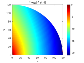
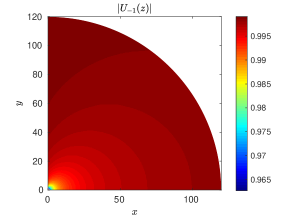
Figure 1: Dynamic ranges of $J_{-1}(z)$ and $U_{-1}(z)$ in $Q$. For comparison purpose, both figures are plotted in the variable $z$.

To this end, we divide $Q$ into several quarter-annulus domains:

$$Q_{i}=\{z\in\mathbb{C}|r_{i}\leq|z|\leq r_{i+1},0\leq\arg{z}\leq\frac{\pi}{2}\},\,\,i=0,\ldots,M-1,\,\,r_{0}=1,r_{M}=R.$$ (19)

We will try to approximate $U_{n}(\nu)$ in each $Q_{i}$ via a modified Laurent series

$$U_{n}(\nu)\simeq L_{n}^{(i)}(\nu)=\sum_{k=-N_{1}}^{N_{2}}d_{k}^{(i)}\nu^{k},\qquad z\in Q_{i}.$$ (20)

As noted before, $U_{n}(\nu)$ satisfies a third order ODE with $0$ and $\infty$ as the only singular points [1, 18]. Thus, $U_{n}(\nu)$ is analytic in $Q_{i}$. By Lemma 2, in order to guarantee the accuracy of the approximation in the whole domain $Q_{i}$, it is sufficient to ensure the same accuracy is achieved on the boundary of $Q_{i}$, i.e.,

$$\left|U_{n}(\nu)-\sum_{k=-N_{1}}^{N_{2}}d_{k}^{(i)}\nu^{k}\right|\leq\epsilon,\qquad z\in\partial Q_{i}.$$ (21)

The error-bound in (21) is achieved by solving the least squares problem

$$\rm{\mathbf{A}}\rm{\mathbf{d}}^{(i)}=\rm{\mathbf{f}},$$ (22)

where

$$A_{jk}=\nu_{j}^{k},\qquad f_{j}=U_{n}(\nu_{j}),\quad j=1,\ldots,4N_{b},$$ (23)

where $\nu_{j}=3(z_{j}/2)^{2/3}$, and $z_{j}$ are chosen to be the images of Gauss-Legendre nodes on each segment of $\partial Q_{i}$, $N_{b}$ is chosen to ensure that the error of approximation of $U_{n}(\nu)$ by the corresponding Legendre polynomial interpolation on each segment of $\partial Q_{i}$ is bounded by $\epsilon$. The right hand side $\rm{\mathbf{f}}$ in (22) is computed via symbolic software system Mathematica to at least $50$ digits. In other words, we do not use the actual analytic Laurent series to approximate $U_{n}$ on each quarter-annulus $Q_{i}$. Instead, a numerical procedure is applied to find much more efficient “modified” Laurent series for approximating $U_{n}$ on each $Q_{i}$.

The linear system (22) is ill-conditioned. However, since we always use $\rm{\mathbf{d}}^{(i)}$ in the modified Laurent series to evaluate $U_{n}$, we will obtain high accuracy in function evaluation in the entire sub-region as long as the residual of the least squares problem (22) is small by the maximum principle.

The least squares solver also reveals the numerical rank of $\rm{\mathbf{A}}$, which is used to obtain the optimal value of $N_{\rm T}=N_{2}-N_{1}+1$, the total number of terms in the modified Laurent series. It is then straightforward to use a simple search to find the value for $N_{1}$, which completes the algorithm for finding a nearly optimal and highly accurate modified Laurent series approximation for $U_{n}$ in $Q_{i}$.

Remark 1.

We would like to emphasize that the modified Laurent series may not be unique, but this non-uniqueness has no effect on the accuracy of the approximation.

Remark 2.

We have computed the integrals

$$I_{n}=\int_{\partial Q}\frac{J_{n}^{\prime}(z)}{J_{n}(z)}dz=-\int_{\partial Q}\frac{J_{n-1}(z)}{J_{n}(z)}dz$$ (24)

for $n=-1,\ldots,2$ and found numerically that they are all close to zero. By the argument principle [5, p. 152], we have

$$I_{n}=2\pi i(Z_{n}-P_{n}),$$ (25)

where $Z_{n}$ and $P_{n}$ denote respectively the number of zeros and poles of $J_{n}(z)$ inside $\partial Q$. Since $J_{n}(z)$ is analytic in $Q$, it has no poles in $Q$, i.e., $P_{n}=0$. Thus, the fact that $I_{n}$ is very close to zero shows that $Z_{n}=0$, that is, $J_{n}$ has no zeros in $Q$. Further numerical investigation shows that $|U_{n}(\nu)|$ ranges from $0.95$ to $1.7$ on $\partial Q$. Combining these two facts, we conclude that the absolute error bound on the approximation of $U_{n}$ gives roughly the same relative error bound.

3.3 Evaluation of $J_{n}$ for $n=-1,\,\ldots,\,2$

Once the coefficients of modified Laurent series for each sub-region are obtained and stored, the evaluation of $J_{n}(z)$ is straightforward. That is, we first compute $|z|$ to decide on which region the point lies, then use the proper representation to evaluate $J_{n}(z)$ accordingly. We summarize the algorithm for calculating $J_{n}(z)$ for $z\in\overline{\mathbb{C}^{+}}$, $n=-1,\,\ldots,\,2$ in Algorithm 1.

Algorithm 1 Evaluation of $J_{n}(z)$ for $z\in\overline{\mathbb{C}^{+}}$

procedure Abram($z$,$f$)

      $\triangleright$ Input parameter: $z$ - the complex number for which the Abramowitz function $J_{n}$ is to be evaluated.

      $\triangleright$ Output parameter: $f$ - the value of Abramowitz function $J_{n}(z)$.

     assert $\mbox{Re}(z)\geq 0$.

     if $|z|\leq 1$ then $\triangleright$ $z$ is in the series expansion region.

         Use the series expansion (6) to evaluate $f=J_{n}(z)$.

     else if $|z|\geq 120$ then $\triangleright$ $z$ is in the asymptotic region.

         Set $\nu=3(z/2)^{2/3}$.

         Use the asymptotic expansion (17) to compute $U_{n}(\nu)$.

         Set $f=\sqrt{\frac{\pi}{3}}\,\left(\frac{\nu}{3}\right)^{n/2}\,e^{-\nu}\,U_{n}(\nu)$.

     else$\triangleright$ $z$ is in the intermediate region.

         Set $\nu=3(z/2)^{2/3}$.

         Use a precomputed modified Laurent series expansion (20) to compute $U_{n}(\nu)$.

         Set $f=\sqrt{\frac{\pi}{3}}\,\left(\frac{\nu}{3}\right)^{n/2}\,e^{-\nu}\,U_{n}(\nu)$.

     end if

end procedure

Remark 3.

All these expansions can be converted into a polynomial of certain transformed variable multiplying with some factor. We use Horner’s method [17, §4.6.4] to evaluate the polynomial in optimal arithmetic operations.

Remark 4.

The accuracy of $J_{n}(z)$ deteriorates as $|z|$ increases since the condition number of evaluating the exponential function $e^{-\nu}$ is $|\nu|$. This is unavoidable in any numerical scheme as the phenomenon is related to physical ill-conditioning of evaluating $J_{n}(z)$ for the argument with large magnitude.

3.4 Evaluation of $J_{n}$ for $n>2$

In [9], it is shown that (4) is stable in both directions when $z$ is a positive real number. We have implemented the forward recurrence to evaluate $J_{n}(z)$ for $n>2$. We have not observed any numerical instability during our numerical tests for $z\in\overline{\mathbb{C}^{+}}$.

4 Numerical results

We have performed numerical experiments on a laptop with a 2.10GHz Intel Core i7-4600U processor and 4GB of RAM.

For the series expansion (6), a straightforward calculation shows that $18$ terms in $\sum b_{k}^{(n)}z^{k}$ and $9$ nonzero terms in $\sum a_{k}^{(n)}z^{k}$ are needed to reach the IEEE extended precision ($\epsilon_{\rm mach}\approx 1.09\cdot 10^{-19}$) for $J_{n}$ ($n=-1,\ldots,2$). For the asymptotic expansion (17), we find that it is sufficient to choose $N_{a}=18$, $R=120$ for the IEEE extended precision. All coefficients are precomputed with $50$ digit precision.

For the intermediate region, we divide $|z|$ on $[1,120]$ into three subintervals $[1,3]$, $[3,15]$, $[15,120]$ and $Q$ into $Q_{1}$, $Q_{2}$, $Q_{3}$, respectively. We use quadruple precision to carry out the precomputation step and solve the least squares problem with $10^{-20}$ accuracy. We have found that for $Q_{1}$ we need $N_{2}=11$, $N_{T}=30$ for $J_{0}$ and $J_{1}$, $N_{2}=10$, $N_{T}=32$ for $J_{-1}$, and $N_{2}=11$, $N_{T}=32$ for $J_{2}$. For all four functions $J_{n}$ ($n=-1,0,1,2$), we need $N_{2}=0$, $N_{T}=30$ for $Q_{2}$ and $N_{2}=0$, $N_{T}=20$ for $Q_{3}$. The coefficients of modified Laurent series for $J_{n}$ ($n=-1,0,1,2$) on $Q_{i}$ ($i=1,2,3$) are listed in Tables 4–15 in B.

Remark 5.

The coefficients in Tables 4–15 for $Q_{2}$ and $Q_{3}$ do not have small norms. However, for $Q_{2}$, $\left|\frac{1}{\nu}\right|\leq\frac{1}{3(3/2)^{(2/3)}}=0.254\ldots$; and for $Q_{3}$, $\left|\frac{1}{\nu}\right|\leq\frac{1}{3(15/2)^{(2/3)}}\approx 0.087$. It is easy to see that terms $c_{j}\left(\frac{1}{\nu}\right)^{j}$ decrease as $j$ increases. Alternatively, we could consider the Laurent series of the form $\sum\tilde{c}_{j}\left(\frac{\nu_{i}}{\nu}\right)^{j}$ with $\nu_{i}=3(r_{i}/2)^{(2/3)}$ ($r_{i}$ is the lower bound for $|z|$ in $Q_{i}$). Then the coefficient vector $\tilde{c}$ will have small norm, as required in [6, 3]. However, this corresponds to the column scaling in the least squares matrix and almost all methods for solving the least squares problems do column normalization. Thus, it has no effect on the accuracy of the solution and stability of the algorithm.

Remark 6.

The partition of the sub-regions is by no means optimal or unique. There is an obvious trade-off between the number of sub-regions and the number of terms in the modified Laurent series (the total number of terms in the modified Laurent expansion slightly increases as the regions gets closer to the origin). This suggests that one may use a finer partition for the regions closer to the origin. We have tried to divide the intermediate region into $14$ regions with $Q_{i}=\{z\in\overline{\mathbb{C}^{+}}|(\sqrt{2})^{i-1}\leq|z|\leq(\sqrt{2})^{i}\}$ ($i=1,\ldots,14$), and we observe that only $20$ terms are needed for all regions. However, our numerical experiments indicate that the partition has little effect on the overall performance (i.e., speed and accuracy) of the algorithm.

We first check the accuracy of Algorithm 1. The reference function values are calculated via Mathematica to at least 50 digit accuracy. The error is measured in terms of maximum relative error, i.e.,

$$E=\max_{i}\frac{|\hat{J}_{n}(z_{i})-\tilde{J}_{n}(z_{i})|}{|\tilde{J}_{n}(z_{i})},$$

where $\tilde{J}_{n}(z_{i})=e^{\nu_{i}}J_{n}(z_{i})$ ($\nu_{i}=3(z_{i}/2)^{2/3}$) is the reference value of the scaled Abramowitz function computed via Mathematica, and $\hat{J}_{n}(z_{i})$ is the value computed via our algorithm. The points $z_{i}$ are sampled randomly with uniform distribution in both its magnitude and angle in $\overline{\mathbb{C}^{+}}$. Table 1 lists the errors for evaluating $\tilde{J}_{n}$ ($n=-1,0,1,2$) in various regions, where we observe that the errors are within $10\epsilon_{\rm mach}$ with the machine epsilon $\epsilon_{\rm mach}\approx 2.22\times 10^{-16}$ for IEEE double precision. In general, the errors in the first intermediate region $Q_{1}$ are slightly bigger due to mild cancellation errors.

Table 1: The relative $L^{\infty}$ error of Algorithm 1 over $100,000$ uniformly distributed random points in $\overline{\mathbb{C}^{+}}$. The reference value is computed via Mathematica to at least 50 digit accuracy. $S$ denotes the series expansion region and $A$ denotes the asymptotic expansion region.

	S	${Q_{1}}$	${Q_{2}}$	${Q_{3}}$	A
${J_{-1}}$	$1.52\text{\times}{10}^{-15}$	$2.10\text{\times}{10}^{-15}$	$4.38\text{\times}{10}^{-16}$	$6.38\text{\times}{10}^{-16}$	$8.64\text{\times}{10}^{-16}$
${J_{0}}$	$1.31\text{\times}{10}^{-15}$	$2.43\text{\times}{10}^{-15}$	$2.21\text{\times}{10}^{-16}$	$2.18\text{\times}{10}^{-16}$	$2.17\text{\times}{10}^{-16}$
${J_{1}}$	$1.06\text{\times}{10}^{-15}$	$2.40\text{\times}{10}^{-15}$	$4.65\text{\times}{10}^{-16}$	$5.96\text{\times}{10}^{-16}$	$7.97\text{\times}{10}^{-16}$
${J_{2}}$	$1.20\text{\times}{10}^{-15}$	$2.93\text{\times}{10}^{-15}$	$5.55\text{\times}{10}^{-16}$	$8.44\text{\times}{10}^{-16}$	$1.17\text{\times}{10}^{-15}$

Since all three representations (i.e., modified Laurent series, series and asymptotic expansions) mainly involve polynomials of degree less than 30, the algorithm takes about constant time per function evaluation in $\overline{\mathbb{C}^{+}}$. We have tested the CPU time of Algorithm 1 for evaluating $\tilde{J_{n}}(z)$ and compared it with that of evaluating the complex exponential $e^{z}$. The results are shown in Table 2. We observe that on average the CPU time of each function evaluation is about four times of that for the complex exponential evaluation.

Table 2: The total CPU time in seconds for evaluating $\tilde{J_{n}(z)}$ using Algorithm 1 and the exponential function $e^{z}$ over $100,000$ uniformly distributed random points in $\overline{\mathbb{C}^{+}}$.

	${J_{-1}(z)}$	${J_{0}(z)}$	${J_{1}(z)}$	${J_{2}(z)}$	${e^{z}}$
${T}$	$3.60\text{\times}{10}^{-02}$	$3.20\text{\times}{10}^{-02}$	$3.60\text{\times}{10}^{-02}$	$3.20\text{\times}{10}^{-02}$	$8.00\text{\times}{10}^{-03}$

For $n>2$, we have tested the stability of the forward recurrence relation (4) for evaluating $J_{n}$ in $\overline{\mathbb{C}^{+}}$. Numerical experiments indicate that the forward recurrence relation is stable in $\overline{\mathbb{C}^{+}}$. The relative errors are shown in Table 3 for a typical run.

Table 3: The maximum relative error for evaluating $J_{100}$ using the forward recurrence relation (4) over $100,000$ uniformly distributed random points in the domain $\{z\in\mathbb{C}|\operatorname{Re}(z)\geq 0,0<|z|<1000\}$. The reference value is calculated using Mathematica with $240$-digit precision arithmetic.

S	${Q_{1}}$	${Q_{2}}$	${Q_{3}}$	A
$1.29\text{\times}{10}^{-15}$	$2.86\text{\times}{10}^{-15}$	$1.26\text{\times}{10}^{-15}$	$2.03\text{\times}{10}^{-15}$	$3.66\text{\times}{10}^{-15}$

5 Conclusions and further discussions

We have designed an efficient and accurate algorithm for the evaluation of Abramowitz functions $J_{n}$ in the right half of the complex plane. Some useful observations in the design of the algorithm are applicable for evaluating many other special functions in the complex domain. First, it is better to pull out the leading asymptotic factor from the given function when $|z|$ is large. Second, the maximum principle reduces the dimensionality of the approximation problem by one. Third, the least squares scheme is generally a reliable and accurate method to find an approximation of a prescribed form. That is, analytical representations should be used with caution even if they are available, as they often lead to large cancellation error or very inefficient approximations or both.

Finally, though we have used truncated Laurent series representation for approximating Abramowitz functions in the intermediate region, there are many other representations for function approximations. This includes truncated series expansion, rational functions (see, for example, [12]), etc. We have actually tested the truncated series expansion in the sub-region (i.e., $Q_{1}$) closest to the origin for $J_{n}$. Our numerical experiments indicate that the performance is about the same as the one presented in this paper.

Appendix A Zeros of $J_{n}(z)$

We have used NIntegrate in Mathematica to evaluate $I_{n}$ defined in (24). When WorkingPrecision is set to $100$, $|I_{n}|$ are about $10^{-59}$ for $n=-1,0,1,2$. When it is set to $200$, the values of $|I_{n}|$ decrease to $10^{-160}$. By the argument priniciple, $I_{n}$ can only take integral multiples of $2\pi i$. Thus, the numerical calculation clearly shows that $J_{n}$ ($n=-1,0,1,2$) have no zeros in the intermediate region $Q$. Analytically, we can only show that $J_{n}$ has no zeros in the sector $|\operatorname{arg}(z)|\leq\frac{\pi}{4}$. The proof is presented below.

Lemma 3.

If $z_{0}\in\mathbb{C}$ is a zero of $J_{n}(z)$, then also $\bar{z}_{0}$.

Proof.

By the integral representation of $J_{n}(z)$ in (1), we have $J_{n}(\bar{z}_{0})=\bar{J}_{n}(z_{0})$ and the lemma follows. ∎

Lemma 4.

Suppose that $n\geq 0$. Then $J_{n}(z)$ has no zero in the sector $|\arg{z}|\leq\frac{\pi}{4}$.

Proof.

Let $z_{0}=x_{0}+iy_{0}\in\overline{\mathbb{C}^{+}}$ be a zero of $J_{n}(z)$. Then by Lemma 3, $\bar{z}_{0}$ is also a zero of $J_{n}(z)$. Consider functions $f(t)=J_{n}(z_{0}t)$ and $g(t)=J_{n}(\bar{z}_{0}t)$. Then $f(1)=g(1)=0$, and $f$, $g$ and their derivatives decay exponentially fast to $0$ as $t\rightarrow\infty$ by the asymptotic expansion (17).

The differential equation (2) implies that

$$tf^{\prime\prime\prime}(t)-(n-1)f^{\prime\prime}(t)+2z_{0}^{2}f(t)=0,$$ (26)

$$tg^{\prime\prime\prime}(t)-(n-1)g^{\prime\prime}(t)+2\bar{z}_{0}^{2}g(t)=0.$$ (27)

Multiplying both sides of (26) by $g$, integrating both sides from $1$ to $\infty$, and performing integration by parts, we obtain

$$0 =\int_{1}^{\infty}[tf^{\prime\prime\prime}g-(n-1)f^{\prime\prime}g+2z_{0}^{2}fg]dt$$ (28)

$$=tgf^{\prime\prime}\bigg{|}_{1}^{\infty}-\int_{1}^{\infty}f^{\prime\prime}(g+g^{\prime}t)dt+\int_{1}^{\infty}[-(n-1)f^{\prime\prime}g+2z_{0}^{2}fg]dt$$

$$=\int_{1}^{\infty}[-tf^{\prime\prime}g^{\prime}-nf^{\prime\prime}g+2z_{0}^{2}fg]dt$$

$$=\int_{1}^{\infty}[-tf^{\prime\prime}g^{\prime}+nf^{\prime}g^{\prime}+2z_{0}^{2}fg]dt.$$

Similarly,

$$0=\int_{1}^{\infty}[-tf^{\prime}g^{\prime\prime}+nf^{\prime}g^{\prime}+2\bar{z}_{0}^{2}fg]dt.$$ (29)

Moreover,

$$\int_{1}^{\infty}[-tf^{\prime}g^{\prime\prime}-tf^{\prime}g^{\prime\prime}]dt =-\int_{1}^{\infty}td(f^{\prime}g^{\prime})$$ (30)

$$=-tf^{\prime}g^{\prime}\bigg{|}_{1}^{\infty}+\int_{1}^{\infty}f^{\prime}g^{\prime}dt$$

$$=f^{\prime}(1)g^{\prime}(1)+\int_{1}^{\infty}f^{\prime}g^{\prime}dt.$$

Adding (28), (29) and using (30) to simplify the result, we obtain

$$0=f^{\prime}(1)g^{\prime}(1)+(2n+1)\int_{1}^{\infty}f^{\prime}g^{\prime}dt+2(z_{0}^{2}+\bar{z}_{0}^{2})\int_{1}^{\infty}fgdt.$$ (31)

Rearranging (31), we have

$$4(y_{0}^{2}-x_{0}^{2})\int_{1}^{\infty}|J_{n}(z_{0}t)|^{2}dt=|z_{0}|^{2}\left|J^{\prime}_{n}(z_{0})\right|^{2}+(2n+1)|z_{0}|^{2}\int_{1}^{\infty}\left|J^{\prime}_{n}(z_{0}t)\right|^{2}dt.$$ (32)

Since the right side of (32) and the integral on its left side are both positive, we must have $y_{0}^{2}-x_{0}^{2}>0$ and the lemma follows. ∎

Lemma 5.

$J_{n}(z)$ has no zero in $D=\{z\in\overline{\mathbb{C}^{+}}||z|>R\}$, where $R$ is sufficiently large.

Proof.

Subtracting (29) from (28), we have

$$0=\int_{1}^{\infty}t(f^{\prime}g^{\prime\prime}-f^{\prime\prime}g^{\prime})dt+2(z_{0}^{2}-\bar{z}_{0}^{2})\int_{1}^{\infty}fgdt.$$ (33)

That is,

$$4x_{0}y_{0}\int_{1}^{\infty}\left|J_{n}(z_{0}t)\right|^{2}dt=|z_{0}|^{2}\int_{1}^{\infty}\operatorname{Im}\left(\bar{z}_{0}tJ_{n-1}(z_{0}t)J_{n-2}(\bar{z}_{0}t)\right)dt.$$ (34)

In the domain $D$, $J_{n}(z)$ is well approximated by the leading term of its asymptotic expansion. Let $z_{0}=r_{0}e^{i\theta_{0}}$ with $r_{0}>0$ and $\theta_{0}\in[-\pi/2,\pi/2]$. Substituting the leading terms of the asymptotic expansions into both sides of (34) and simplifying the resulting expressions, we obtain

$$\sin(2\theta_{0})\sim-\sin(2\theta_{0}/3).$$ (35)

In other words, two sides of (34) have opposite sign unless they are both equal to zero, i.e., unless $\theta_{0}=0$ or $z_{0}$ is a positive real number. However, $J_{n}(x)>0$ when $x>0$, as seen from its integral representation (1). And the lemma follows. ∎

Appendix B The coefficients of modified Laurent series for $J_{n}$

We list the coefficients $c_{j}$ of modified Laurent series for evaluating $J_{n}$ ($n=-1$, 0, 1, and 2) on each quarter-annulus domain $Q_{i}$ ($i=1$, 2, and 3) in Tables 4–15. That is,

$$J_{n}(z)\approx\sqrt{\frac{\pi}{3}}\left(\frac{\nu}{3}\right)^{n/2}e^{-\nu}\nu^{N_{2}}\sum_{j=0}^{N_{T}-1}c_{j}\left(\frac{1}{\nu}\right)^{j},$$ (36)

where $\nu:=3\left(\frac{z}{2}\right)^{2/3}$. (36) is obtained by combining (5) and (20), and rewriting the modified Laurent series as a power series in $\frac{1}{\nu}$ by pulling out the factor $\nu^{N_{2}}$.

Table 4: The coefficients $c_{j}$ ($j=0,\,\ldots,\,31$) of the modified Laurent series given by (36) to evaluate $J_{-1}(z)$ to $19$-digit precision in $Q_{1}:=\{z\in\mathbb{C}\,|\,\operatorname{Re}(z)\geq 0,\operatorname{Im}(z)\geq 0,1\leq|z|\leq 3\}$. $N_{2}=10$.

real part	imaginary part
$0.508\,404\,632\,082\,606\,781\,52\text{\times}{10}^{-17}$	$-0.174\,608\,152\,994\,637\,499\,48\text{\times}{10}^{-15}$
$-0.745\,912\,235\,026\,426\,206\,60\text{\times}{10}^{-14}$	$0.124\,626\,002\,002\,964\,530\,12\text{\times}{10}^{-13}$
$0.510\,342\,448\,563\,248\,242\,07\text{\times}{10}^{-12}$	$-0.294\,298\,471\,469\,682\,176\,69\text{\times}{10}^{-12}$
$-0.155\,278\,534\,850\,271\,007\,09\text{\times}{10}^{-10}$	$0.263\,158\,514\,306\,763\,567\,96\text{\times}{10}^{-12}$
$0.264\,414\,045\,122\,879\,630\,95\text{\times}{10}^{-09}$	$0.139\,834\,751\,397\,682\,449\,07\text{\times}{10}^{-09}$
$-0.247\,487\,638\,713\,530\,933\,63\text{\times}{10}^{-08}$	$-0.374\,213\,198\,230\,171\,159\,33\text{\times}{10}^{-08}$
$0.482\,268\,582\,740\,909\,041\,08\text{\times}{10}^{-08}$	$0.543\,401\,289\,326\,601\,410\,72\text{\times}{10}^{-07}$
$0.216\,253\,553\,725\,866\,075\,08\text{\times}{10}^{-06}$	$-0.508\,720\,998\,708\,511\,613\,98\text{\times}{10}^{-06}$
$-0.368\,717\,051\,178\,481\,237\,97\text{\times}{10}^{-05}$	$0.301\,340\,166\,557\,595\,939\,20\text{\times}{10}^{-05}$
$0.346\,284\,048\,895\,070\,301\,60\text{\times}{10}^{-04}$	$-0.739\,108\,230\,704\,056\,172\,19\text{\times}{10}^{-05}$
$0.999\,777\,374\,590\,696\,606\,94\text{\times}{10}^{00}$	$-0.576\,030\,836\,245\,300\,251\,51\text{\times}{10}^{-04}$
$-0.823\,278\,581\,628\,196\,930\,45\text{\times}{10}^{-01}$	$0.849\,768\,580\,372\,614\,021\,53\text{\times}{10}^{-03}$
$0.619\,747\,893\,545\,737\,665\,66\text{\times}{10}^{-03}$	$-0.605\,139\,381\,903\,151\,159\,82\text{\times}{10}^{-02}$
$0.566\,151\,822\,947\,680\,796\,37\text{\times}{10}^{-01}$	$0.302\,907\,889\,349\,127\,277\,55\text{\times}{10}^{-01}$
$-0.135\,136\,779\,991\,090\,296\,79\text{\times}{10}^{00}$	$-0.115\,958\,015\,111\,906\,821\,78\text{\times}{10}^{00}$
$0.209\,718\,152\,961\,885\,801\,67\text{\times}{10}^{00}$	$0.349\,173\,944\,608\,271\,288\,28\text{\times}{10}^{00}$
$-0.135\,593\,023\,999\,587\,351\,43\text{\times}{10}^{00}$	$-0.830\,316\,528\,148\,841\,088\,13\text{\times}{10}^{00}$
$-0.399\,898\,988\,541\,072\,716\,42\text{\times}{10}^{00}$	$0.153\,226\,178\,650\,705\,161\,48\text{\times}{10}^{01}$
$0.173\,982\,716\,383\,338\,408\,50\text{\times}{10}^{01}$	$-0.207\,207\,422\,408\,323\,786\,54\text{\times}{10}^{01}$
$-0.382\,180\,642\,772\,971\,751\,42\text{\times}{10}^{01}$	$0.166\,556\,450\,780\,677\,180\,66\text{\times}{10}^{01}$
$0.574\,046\,443\,633\,433\,309\,31\text{\times}{10}^{01}$	$0.364\,413\,737\,004\,387\,528\,95\text{\times}{10}^{00}$
$-0.602\,185\,574\,538\,225\,680\,30\text{\times}{10}^{01}$	$-0.366\,998\,894\,320\,715\,544\,24\text{\times}{10}^{01}$
$0.386\,640\,982\,933\,784\,632\,50\text{\times}{10}^{01}$	$0.656\,323\,653\,065\,047\,142\,02\text{\times}{10}^{01}$
$-0.256\,979\,491\,396\,712\,909\,42\text{\times}{10}^{00}$	$-0.717\,303\,344\,007\,278\,311\,01\text{\times}{10}^{01}$
$-0.261\,383\,686\,683\,662\,857\,52\text{\times}{10}^{01}$	$0.521\,017\,298\,717\,892\,892\,59\text{\times}{10}^{01}$
$0.331\,280\,620\,490\,481\,945\,83\text{\times}{10}^{01}$	$-0.227\,447\,202\,390\,353\,554\,39\text{\times}{10}^{01}$
$-0.229\,475\,501\,388\,204\,966\,70\text{\times}{10}^{01}$	$0.218\,248\,685\,401\,302\,644\,77\text{\times}{10}^{00}$
$0.979\,988\,419\,462\,684\,815\,18\text{\times}{10}^{00}$	$0.430\,819\,146\,717\,141\,565\,57\text{\times}{10}^{00}$
$-0.232\,732\,788\,689\,187\,012\,41\text{\times}{10}^{00}$	$-0.308\,816\,943\,645\,394\,016\,56\text{\times}{10}^{00}$
$0.135\,738\,167\,246\,491\,846\,59\text{\times}{10}^{-01}$	$0.101\,035\,914\,706\,240\,915\,10\text{\times}{10}^{00}$
$0.647\,176\,653\,107\,878\,954\,82\text{\times}{10}^{-02}$	$-0.162\,049\,762\,735\,533\,721\,87\text{\times}{10}^{-01}$
$-0.113\,530\,822\,404\,964\,078\,13\text{\times}{10}^{-02}$	$0.911\,116\,455\,095\,110\,768\,69\text{\times}{10}^{-03}$

Table 5: Similar to Table 4, $c_{j}$ ($j=0,\,\ldots,\,29$) for $J_{-1}(z)$ in $Q_{2}=\{z\in\mathbb{C}\,|\,\operatorname{Re}(z)\geq 0,\operatorname{Im}(z)\geq 0,3\leq|z|\leq 15\}$. $N_{2}=0$.

real part	imaginary part
$0.999\,999\,999\,999\,961\,653\,01\text{\times}{10}^{00}$	$0.141\,806\,832\,347\,584\,925\,36\text{\times}{10}^{-12}$
$-0.833\,333\,333\,158\,883\,431\,56\text{\times}{10}^{-01}$	$-0.183\,554\,755\,025\,424\,015\,39\text{\times}{10}^{-10}$
$0.347\,222\,020\,992\,143\,062\,18\text{\times}{10}^{-02}$	$0.664\,295\,120\,902\,317\,816\,28\text{\times}{10}^{-09}$
$0.554\,592\,179\,369\,355\,251\,95\text{\times}{10}^{-01}$	$0.192\,090\,703\,259\,659\,827\,96\text{\times}{10}^{-07}$
$-0.174\,770\,093\,094\,885\,488\,35\text{\times}{10}^{00}$	$-0.272\,358\,724\,156\,552\,434\,93\text{\times}{10}^{-05}$
$0.475\,579\,850\,792\,853\,198\,78\text{\times}{10}^{00}$	$0.123\,293\,398\,001\,490\,185\,87\text{\times}{10}^{-03}$
$-0.120\,447\,196\,014\,882\,443\,81\text{\times}{10}^{01}$	$-0.333\,799\,891\,312\,548\,583\,84\text{\times}{10}^{-02}$
$0.241\,605\,349\,770\,769\,985\,85\text{\times}{10}^{01}$	$0.599\,204\,046\,472\,687\,860\,33\text{\times}{10}^{-01}$
$0.714\,019\,341\,240\,202\,213\,24\text{\times}{10}^{00}$	$-0.697\,646\,996\,515\,841\,414\,17\text{\times}{10}^{00}$
$-0.603\,675\,406\,822\,103\,741\,45\text{\times}{10}^{02}$	$0.386\,077\,962\,390\,076\,721\,58\text{\times}{10}^{01}$
$0.605\,451\,350\,482\,099\,861\,87\text{\times}{10}^{03}$	$0.324\,292\,794\,756\,158\,453\,98\text{\times}{10}^{02}$
$-0.459\,463\,671\,083\,445\,667\,27\text{\times}{10}^{04}$	$-0.108\,419\,490\,933\,568\,204\,60\text{\times}{10}^{04}$
$0.283\,585\,737\,521\,554\,577\,24\text{\times}{10}^{05}$	$0.147\,667\,142\,274\,551\,196\,33\text{\times}{10}^{05}$
$-0.135\,548\,409\,522\,738\,422\,75\text{\times}{10}^{06}$	$-0.136\,296\,993\,207\,088\,386\,68\text{\times}{10}^{06}$
$0.427\,223\,358\,854\,162\,769\,83\text{\times}{10}^{06}$	$0.936\,405\,385\,625\,510\,558\,57\text{\times}{10}^{06}$
$-0.187\,177\,344\,190\,171\,379\,32\text{\times}{10}^{06}$	$-0.490\,146\,368\,535\,523\,402\,06\text{\times}{10}^{07}$
$-0.766\,746\,981\,331\,305\,086\,47\text{\times}{10}^{07}$	$0.192\,939\,969\,196\,334\,868\,42\text{\times}{10}^{08}$
$0.566\,216\,201\,198\,774\,900\,02\text{\times}{10}^{08}$	$-0.533\,796\,877\,619\,324\,138\,68\text{\times}{10}^{08}$
$-0.245\,446\,260\,540\,985\,694\,13\text{\times}{10}^{09}$	$0.769\,699\,843\,063\,185\,308\,11\text{\times}{10}^{08}$
$0.736\,524\,060\,830\,223\,396\,55\text{\times}{10}^{09}$	$0.118\,988\,708\,450\,170\,908\,57\text{\times}{10}^{09}$
$-0.152\,002\,939\,636\,990\,115\,85\text{\times}{10}^{10}$	$-0.111\,677\,447\,076\,659\,508\,37\text{\times}{10}^{10}$
$0.181\,576\,363\,392\,016\,524\,60\text{\times}{10}^{10}$	$0.370\,018\,124\,502\,864\,503\,98\text{\times}{10}^{10}$
$0.236\,970\,051\,052\,140\,740\,56\text{\times}{10}^{09}$	$-0.769\,732\,352\,121\,328\,283\,29\text{\times}{10}^{10}$
$-0.605\,418\,652\,742\,096\,914\,12\text{\times}{10}^{10}$	$0.105\,094\,370\,501\,909\,818\,95\text{\times}{10}^{11}$
$0.134\,473\,475\,911\,834\,175\,29\text{\times}{10}^{11}$	$-0.828\,696\,601\,026\,570\,423\,17\text{\times}{10}^{10}$
$-0.165\,386\,003\,269\,058\,328\,99\text{\times}{10}^{11}$	$0.878\,893\,331\,337\,860\,555\,48\text{\times}{10}^{09}$
$0.121\,080\,386\,549\,490\,128\,13\text{\times}{10}^{11}$	$0.583\,201\,605\,488\,309\,253\,71\text{\times}{10}^{10}$
$-0.458\,813\,237\,705\,320\,160\,82\text{\times}{10}^{10}$	$-0.645\,912\,107\,582\,825\,318\,47\text{\times}{10}^{10}$
$0.335\,597\,695\,613\,487\,923\,57\text{\times}{10}^{09}$	$0.300\,129\,749\,468\,952\,920\,83\text{\times}{10}^{10}$
$0.215\,904\,420\,673\,766\,075\,26\text{\times}{10}^{09}$	$-0.515\,536\,276\,388\,964\,358\,29\text{\times}{10}^{09}$

Table 6: Similar to Table 4, $c_{j}$ ($j=0,\,\ldots,\,19$) for $J_{-1}(z)$ in $Q_{3}=\{z\in\mathbb{C}\,|\,\operatorname{Re}(z)\geq 0,\operatorname{Im}(z)\geq 0,15\leq|z|\leq 120\}$. $N_{2}=0$.

real part	imaginary part
$0.100\,000\,000\,000\,000\,002\,11\text{\times}{10}^{01}$	$0.178\,673\,059\,693\,174\,710\,10\text{\times}{10}^{-16}$
$-0.833\,333\,333\,333\,370\,624\,47\text{\times}{10}^{-01}$	$-0.977\,231\,664\,374\,838\,609\,03\text{\times}{10}^{-14}$
$0.347\,222\,222\,196\,623\,078\,73\text{\times}{10}^{-02}$	$0.185\,750\,995\,314\,155\,635\,50\text{\times}{10}^{-11}$
$0.554\,591\,050\,637\,792\,915\,69\text{\times}{10}^{-01}$	$-0.170\,367\,606\,540\,725\,010\,33\text{\times}{10}^{-09}$
$-0.174\,766\,524\,353\,726\,066\,09\text{\times}{10}^{00}$	$0.720\,973\,568\,196\,242\,083\,86\text{\times}{10}^{-08}$
$0.475\,521\,803\,699\,479\,611\,03\text{\times}{10}^{00}$	$0.458\,867\,227\,971\,042\,147\,45\text{\times}{10}^{-07}$
$-0.120\,457\,482\,849\,866\,306\,05\text{\times}{10}^{01}$	$-0.234\,325\,765\,233\,684\,458\,86\text{\times}{10}^{-04}$
$0.244\,764\,600\,694\,641\,417\,08\text{\times}{10}^{01}$	$0.144\,884\,043\,026\,931\,818\,55\text{\times}{10}^{-02}$
$-0.194\,435\,702\,473\,795\,297\,07\text{\times}{10}^{00}$	$-0.512\,841\,062\,799\,477\,565\,51\text{\times}{10}^{-01}$
$-0.447\,750\,705\,123\,945\,998\,08\text{\times}{10}^{02}$	$0.119\,733\,980\,838\,481\,655\,62\text{\times}{10}^{01}$
$0.421\,634\,597\,094\,092\,230\,79\text{\times}{10}^{03}$	$-0.187\,325\,842\,170\,831\,902\,17\text{\times}{10}^{02}$
$-0.309\,908\,462\,261\,138\,328\,47\text{\times}{10}^{04}$	$0.180\,645\,013\,045\,163\,968\,11\text{\times}{10}^{03}$
$0.209\,138\,849\,163\,905\,853\,68\text{\times}{10}^{05}$	$-0.592\,962\,111\,536\,245\,581\,48\text{\times}{10}^{03}$
$-0.128\,959\,963\,550\,548\,747\,85\text{\times}{10}^{06}$	$-0.108\,214\,826\,602\,820\,261\,69\text{\times}{10}^{05}$
$0.670\,852\,955\,256\,816\,110\,41\text{\times}{10}^{06}$	$0.198\,088\,627\,508\,652\,376\,78\text{\times}{10}^{06}$
$-0.263\,378\,771\,825\,866\,161\,50\text{\times}{10}^{07}$	$-0.168\,133\,321\,132\,881\,930\,78\text{\times}{10}^{07}$
$0.670\,963\,418\,948\,175\,610\,42\text{\times}{10}^{07}$	$0.859\,319\,504\,013\,814\,145\,32\text{\times}{10}^{07}$
$-0.765\,712\,819\,081\,208\,414\,43\text{\times}{10}^{07}$	$-0.265\,726\,278\,587\,171\,822\,34\text{\times}{10}^{08}$
$-0.598\,034\,480\,268\,757\,485\,09\text{\times}{10}^{07}$	$0.448\,016\,842\,841\,870\,047\,03\text{\times}{10}^{08}$
$0.192\,093\,223\,477\,658\,710\,37\text{\times}{10}^{08}$	$-0.300\,660\,136\,102\,592\,770\,74\text{\times}{10}^{08}$

Table 7: The coefficients $c_{j}$ ($j=0,\,\ldots,\,29$) of the modified Laurent series given by (36) to evaluate $J_{0}(z)$ to $19$-digit precision in $Q_{1}:=\{z\in\mathbb{C}\,|\,\operatorname{Re}(z)\geq 0,\operatorname{Im}(z)\geq 0,1\leq|z|\leq 3\}$. $N_{2}=11$.

real part	imaginary part
$-0.908\,326\,076\,414\,336\,267\,23\text{\times}{10}^{-16}$	$-0.129\,717\,168\,574\,382\,531\,77\text{\times}{10}^{-15}$
$0.123\,898\,046\,202\,308\,783\,43\text{\times}{10}^{-14}$	$0.123\,740\,863\,457\,694\,755\,60\text{\times}{10}^{-13}$
$0.189\,256\,659\,364\,469\,738\,63\text{\times}{10}^{-12}$	$-0.435\,940\,424\,250\,019\,098\,08\text{\times}{10}^{-12}$
$-0.934\,361\,246\,990\,827\,287\,82\text{\times}{10}^{-11}$	$0.716\,102\,401\,714\,559\,472\,15\text{\times}{10}^{-11}$
$0.210\,054\,713\,734\,263\,561\,92\text{\times}{10}^{-09}$	$-0.315\,707\,201\,005\,084\,973\,22\text{\times}{10}^{-10}$
$-0.279\,214\,696\,044\,122\,838\,31\text{\times}{10}^{-08}$	$-0.102\,677\,547\,667\,761\,081\,85\text{\times}{10}^{-08}$
$0.222\,106\,972\,868\,927\,816\,43\text{\times}{10}^{-07}$	$0.252\,819\,612\,779\,334\,845\,78\text{\times}{10}^{-07}$
$-0.714\,946\,136\,758\,798\,733\,72\text{\times}{10}^{-07}$	$-0.307\,710\,587\,817\,158\,724\,27\text{\times}{10}^{-06}$
$-0.639\,545\,392\,172\,864\,365\,91\text{\times}{10}^{-06}$	$0.242\,649\,612\,156\,418\,576\,61\text{\times}{10}^{-05}$
$0.114\,775\,999\,343\,307\,552\,36\text{\times}{10}^{-04}$	$-0.126\,927\,831\,114\,001\,418\,26\text{\times}{10}^{-04}$
$-0.944\,476\,013\,855\,187\,381\,18\text{\times}{10}^{-04}$	$0.365\,821\,223\,604\,423\,130\,63\text{\times}{10}^{-04}$
$0.100\,052\,271\,314\,163\,894\,19\text{\times}{10}^{01}$	$0.425\,276\,796\,329\,337\,906\,45\text{\times}{10}^{-04}$
$-0.854\,163\,396\,955\,419\,739\,74\text{\times}{10}^{-01}$	$-0.116\,682\,742\,755\,977\,009\,74\text{\times}{10}^{-02}$
$0.926\,800\,887\,589\,574\,990\,03\text{\times}{10}^{-01}$	$0.755\,251\,304\,311\,641\,080\,91\text{\times}{10}^{-02}$
$-0.128\,309\,621\,833\,997\,329\,14\text{\times}{10}^{00}$	$-0.319\,992\,796\,723\,225\,875\,69\text{\times}{10}^{-01}$
$0.182\,628\,019\,024\,601\,056\,36\text{\times}{10}^{00}$	$0.101\,126\,017\,894\,517\,862\,53\text{\times}{10}^{00}$
$-0.220\,865\,249\,636\,184\,775\,05\text{\times}{10}^{00}$	$-0.247\,947\,862\,302\,196\,466\,77\text{\times}{10}^{00}$
$0.167\,009\,795\,045\,197\,070\,12\text{\times}{10}^{00}$	$0.475\,744\,612\,834\,386\,536\,40\text{\times}{10}^{00}$
$0.622\,308\,413\,429\,398\,471\,77\text{\times}{10}^{-01}$	$-0.705\,468\,982\,760\,372\,689\,06\text{\times}{10}^{00}$
$-0.461\,605\,904\,356\,603\,013\,33\text{\times}{10}^{00}$	$0.774\,053\,364\,314\,386\,650\,12\text{\times}{10}^{00}$
$0.862\,829\,051\,456\,672\,618\,61\text{\times}{10}^{00}$	$-0.548\,832\,850\,036\,770\,366\,33\text{\times}{10}^{00}$
$-0.101\,577\,254\,090\,500\,611\,78\text{\times}{10}^{01}$	$0.896\,535\,548\,331\,156\,865\,88\text{\times}{10}^{-01}$
$0.811\,270\,429\,332\,580\,731\,93\text{\times}{10}^{00}$	$0.342\,234\,269\,766\,613\,927\,85\text{\times}{10}^{00}$
$-0.405\,888\,707\,807\,449\,413\,28\text{\times}{10}^{00}$	$-0.504\,149\,505\,276\,123\,586\,37\text{\times}{10}^{00}$
$0.706\,462\,957\,702\,165\,180\,95\text{\times}{10}^{-01}$	$0.390\,200\,539\,029\,643\,279\,00\text{\times}{10}^{00}$
$0.625\,762\,782\,072\,074\,916\,89\text{\times}{10}^{-01}$	$-0.186\,652\,488\,193\,406\,157\,55\text{\times}{10}^{00}$
$-0.560\,694\,637\,461\,569\,905\,40\text{\times}{10}^{-01}$	$0.513\,693\,450\,241\,894\,804\,53\text{\times}{10}^{-01}$
$0.208\,545\,650\,595\,933\,312\,01\text{\times}{10}^{-01}$	$-0.496\,224\,602\,988\,077\,610\,80\text{\times}{10}^{-02}$
$-0.377\,364\,113\,716\,308\,568\,48\text{\times}{10}^{-02}$	$-0.107\,066\,204\,275\,949\,726\,34\text{\times}{10}^{-02}$
$0.246\,580\,628\,163\,009\,904\,62\text{\times}{10}^{-03}$	$0.247\,935\,486\,569\,863\,450\,25\text{\times}{10}^{-03}$

Table 8: Similar to Table 7, $c_{j}$ ($j=0,\,\ldots,\,29$) for $J_{0}(z)$ in $Q_{2}:=\{z\in\mathbb{C}\,|\,\operatorname{Re}(z)\geq 0,\operatorname{Im}(z)\geq 0,3\leq|z|\leq 15\}$. $N_{2}=0$.

real part	imaginary part
$0.999\,999\,999\,999\,886\,372\,17\text{\times}{10}^{00}$	$-0.866\,354\,009\,393\,752\,328\,46\text{\times}{10}^{-13}$
$-0.833\,333\,333\,231\,314\,999\,72\text{\times}{10}^{-01}$	$0.225\,193\,216\,710\,240\,252\,50\text{\times}{10}^{-10}$
$0.868\,055\,556\,894\,298\,268\,98\text{\times}{10}^{-01}$	$-0.207\,344\,975\,804\,416\,979\,38\text{\times}{10}^{-08}$
$-0.118\,152\,065\,141\,757\,379\,47\text{\times}{10}^{00}$	$0.963\,392\,704\,416\,303\,720\,77\text{\times}{10}^{-07}$
$0.179\,693\,330\,571\,877\,776\,54\text{\times}{10}^{00}$	$-0.230\,570\,436\,517\,271\,579\,18\text{\times}{10}^{-05}$
$-0.243\,373\,421\,697\,903\,758\,42\text{\times}{10}^{00}$	$0.980\,983\,545\,245\,184\,539\,57\text{\times}{10}^{-05}$
$0.147\,644\,294\,738\,726\,207\,63\text{\times}{10}^{-01}$	$0.127\,823\,214\,509\,188\,570\,49\text{\times}{10}^{-02}$
$0.233\,096\,279\,379\,025\,075\,55\text{\times}{10}^{01}$	$-0.510\,737\,071\,722\,602\,207\,79\text{\times}{10}^{-01}$
$-0.164\,809\,814\,902\,887\,641\,06\text{\times}{10}^{02}$	$0.112\,915\,858\,278\,761\,992\,38\text{\times}{10}^{01}$
$0.923\,051\,175\,444\,476\,845\,20\text{\times}{10}^{02}$	$-0.172\,620\,962\,517\,061\,806\,00\text{\times}{10}^{02}$
$-0.516\,004\,179\,227\,537\,180\,15\text{\times}{10}^{03}$	$0.193\,287\,527\,641\,909\,072\,74\text{\times}{10}^{03}$
$0.324\,649\,316\,911\,391\,059\,61\text{\times}{10}^{04}$	$-0.159\,010\,533\,363\,178\,438\,19\text{\times}{10}^{04}$
$-0.223\,140\,605\,129\,205\,983\,45\text{\times}{10}^{05}$	$0.905\,996\,631\,238\,433\,354\,41\text{\times}{10}^{04}$
$0.146\,047\,082\,313\,218\,996\,14\text{\times}{10}^{06}$	$-0.262\,333\,230\,398\,374\,376\,29\text{\times}{10}^{05}$
$-0.811\,455\,137\,409\,768\,033\,11\text{\times}{10}^{06}$	$-0.981\,048\,077\,563\,203\,440\,84\text{\times}{10}^{05}$
$0.354\,579\,713\,045\,832\,193\,48\text{\times}{10}^{07}$	$0.182\,949\,487\,040\,402\,647\,18\text{\times}{10}^{07}$
$-0.110\,840\,573\,517\,255\,386\,29\text{\times}{10}^{08}$	$-0.131\,701\,608\,090\,555\,575\,56\text{\times}{10}^{08}$
$0.179\,467\,425\,877\,273\,553\,94\text{\times}{10}^{08}$	$0.629\,866\,054\,852\,320\,280\,06\text{\times}{10}^{08}$
$0.358\,000\,946\,662\,486\,988\,96\text{\times}{10}^{08}$	$-0.216\,144\,510\,814\,329\,451\,59\text{\times}{10}^{09}$
$-0.373\,049\,554\,275\,698\,007\,21\text{\times}{10}^{09}$	$0.521\,946\,990\,726\,741\,182\,29\text{\times}{10}^{09}$
$0.144\,794\,204\,884\,510\,587\,53\text{\times}{10}^{10}$	$-0.758\,676\,929\,174\,929\,413\,54\text{\times}{10}^{09}$
$-0.359\,517\,888\,165\,641\,668\,63\text{\times}{10}^{10}$	$0.226\,183\,986\,965\,801\,840\,17\text{\times}{10}^{08}$
$0.600\,011\,150\,215\,066\,620\,33\text{\times}{10}^{10}$	$0.310\,062\,196\,048\,266\,214\,51\text{\times}{10}^{10}$
$-0.607\,805\,483\,326\,699\,743\,19\text{\times}{10}^{10}$	$-0.878\,915\,487\,267\,611\,439\,21\text{\times}{10}^{10}$
$0.155\,762\,429\,613\,365\,664\,25\text{\times}{10}^{10}$	$0.138\,851\,365\,499\,019\,567\,58\text{\times}{10}^{11}$
$0.552\,500\,835\,985\,386\,752\,66\text{\times}{10}^{10}$	$-0.136\,224\,965\,335\,758\,282\,28\text{\times}{10}^{11}$
$-0.926\,257\,609\,344\,894\,116\,55\text{\times}{10}^{10}$	$0.757\,327\,801\,853\,722\,127\,72\text{\times}{10}^{10}$
$0.695\,430\,356\,361\,424\,397\,47\text{\times}{10}^{10}$	$-0.128\,503\,666\,477\,737\,995\,33\text{\times}{10}^{10}$
$-0.256\,305\,707\,649\,161\,100\,06\text{\times}{10}^{10}$	$-0.855\,417\,514\,506\,914\,240\,86\text{\times}{10}^{09}$
$0.338\,633\,522\,975\,537\,085\,94\text{\times}{10}^{09}$	$0.369\,396\,907\,511\,817\,802\,09\text{\times}{10}^{09}$

Table 9: Similar to Table 7, $c_{j}$ ($j=0,\,\ldots,\,19$) for $J_{0}(z)$ in $Q_{3}:=\{z\in\mathbb{C}\,|\,\operatorname{Re}(z)\geq 0,\operatorname{Im}(z)\geq 0,15\leq|z|\leq 120\}$. $N_{2}=0$.

real part	imaginary part
$0.999\,999\,999\,999\,999\,969\,30\text{\times}{10}^{00}$	$0.175\,938\,640\,339\,119\,357\,46\text{\times}{10}^{-16}$
$-0.833\,333\,333\,333\,199\,009\,02\text{\times}{10}^{-01}$	$-0.168\,461\,478\,982\,929\,779\,50\text{\times}{10}^{-15}$
$0.868\,055\,555\,534\,238\,161\,81\text{\times}{10}^{-01}$	$-0.114\,533\,947\,041\,601\,480\,63\text{\times}{10}^{-11}$
$-0.118\,152\,006\,023\,476\,722\,98\text{\times}{10}^{00}$	$0.230\,483\,859\,692\,902\,846\,78\text{\times}{10}^{-09}$
$0.179\,689\,507\,723\,700\,402\,85\text{\times}{10}^{00}$	$-0.219\,453\,859\,989\,587\,483\,45\text{\times}{10}^{-07}$
$-0.243\,237\,776\,508\,143\,247\,72\text{\times}{10}^{00}$	$0.120\,879\,546\,268\,738\,763\,83\text{\times}{10}^{-05}$
$0.117\,005\,703\,951\,529\,384\,11\text{\times}{10}^{-01}$	$-0.381\,038\,547\,987\,292\,836\,35\text{\times}{10}^{-04}$
$0.237\,452\,068\,486\,745\,862\,41\text{\times}{10}^{01}$	$0.413\,464\,001\,734\,930\,254\,58\text{\times}{10}^{-03}$
$-0.167\,588\,370\,665\,203\,899\,57\text{\times}{10}^{02}$	$0.204\,376\,305\,776\,969\,609\,42\text{\times}{10}^{-01}$
$0.889\,665\,457\,654\,216\,509\,42\text{\times}{10}^{02}$	$-0.120\,643\,172\,387\,860\,813\,73\text{\times}{10}^{01}$
$-0.394\,943\,740\,653\,525\,533\,20\text{\times}{10}^{03}$	$0.339\,120\,804\,377\,190\,498\,06\text{\times}{10}^{02}$
$0.140\,598\,972\,643\,933\,533\,50\text{\times}{10}^{04}$	$-0.624\,748\,204\,647\,099\,272\,86\text{\times}{10}^{03}$
$-0.404\,513\,553\,220\,860\,199\,35\text{\times}{10}^{04}$	$0.808\,763\,586\,506\,789\,969\,96\text{\times}{10}^{04}$
$0.193\,845\,431\,043\,598\,119\,33\text{\times}{10}^{05}$	$-0.745\,595\,997\,903\,222\,393\,86\text{\times}{10}^{05}$
$-0.205\,176\,883\,526\,801\,360\,30\text{\times}{10}^{06}$	$0.480\,862\,899\,008\,954\,123\,20\text{\times}{10}^{06}$
$0.170\,435\,218\,408\,308\,883\,84\text{\times}{10}^{07}$	$-0.205\,186\,473\,609\,185\,214\,09\text{\times}{10}^{07}$
$-0.877\,050\,770\,331\,537\,793\,72\text{\times}{10}^{07}$	$0.499\,039\,829\,050\,756\,294\,08\text{\times}{10}^{07}$
$0.267\,971\,952\,909\,986\,438\,93\text{\times}{10}^{08}$	$-0.308\,748\,073\,455\,144\,363\,82\text{\times}{10}^{07}$
$-0.434\,487\,954\,511\,809\,855\,46\text{\times}{10}^{08}$	$-0.141\,981\,907\,205\,855\,775\,90\text{\times}{10}^{08}$
$0.266\,930\,744\,198\,889\,886\,36\text{\times}{10}^{08}$	$0.256\,745\,115\,830\,298\,117\,22\text{\times}{10}^{08}$

Table 10: The coefficients $c_{j}$ ($j=0,\,\ldots,\,29$) of the modified Laurent series given by (36) for evaluation of $J_{1}(z)$ to $19$-digit precision in $Q_{1}:=\{z\in\mathbb{C}\,|\,\operatorname{Re}(z)\geq 0,\operatorname{Im}(z)\geq 0,1\leq|z|\leq 3\}$. $N_{2}=11$.

real part	imaginary part
$0.110\,051\,983\,428\,464\,857\,55\text{\times}{10}^{-15}$	$-0.694\,974\,798\,976\,949\,017\,98\text{\times}{10}^{-16}$
$-0.102\,537\,173\,909\,528\,367\,50\text{\times}{10}^{-13}$	$0.573\,447\,330\,612\,984\,007\,54\text{\times}{10}^{-15}$
$0.355\,419\,807\,461\,472\,502\,13\text{\times}{10}^{-12}$	$0.171\,380\,359\,477\,394\,369\,87\text{\times}{10}^{-12}$
$-0.570\,656\,634\,267\,733\,169\,25\text{\times}{10}^{-11}$	$-0.800\,977\,526\,803\,848\,613\,53\text{\times}{10}^{-11}$
$0.213\,779\,424\,023\,220\,328\,01\text{\times}{10}^{-10}$	$0.177\,457\,611\,434\,888\,666\,34\text{\times}{10}^{-09}$
$0.925\,041\,777\,735\,636\,816\,59\text{\times}{10}^{-09}$	$-0.234\,916\,902\,824\,469\,120\,66\text{\times}{10}^{-08}$
$-0.219\,581\,322\,067\,737\,848\,69\text{\times}{10}^{-07}$	$0.187\,152\,555\,411\,620\,792\,36\text{\times}{10}^{-07}$
$0.267\,441\,468\,134\,350\,880\,20\text{\times}{10}^{-06}$	$-0.605\,381\,927\,275\,615\,665\,71\text{\times}{10}^{-07}$
$-0.214\,179\,643\,388\,840\,263\,93\text{\times}{10}^{-05}$	$-0.551\,667\,774\,710\,601\,484\,67\text{\times}{10}^{-06}$
$0.116\,052\,298\,034\,036\,980\,59\text{\times}{10}^{-04}$	$0.100\,892\,068\,271\,577\,766\,27\text{\times}{10}^{-04}$
$-0.369\,022\,862\,459\,559\,263\,31\text{\times}{10}^{-04}$	$-0.857\,345\,236\,304\,648\,588\,44\text{\times}{10}^{-04}$
$0.999\,988\,860\,265\,205\,370\,47\text{\times}{10}^{00}$	$0.499\,847\,603\,957\,965\,000\,59\text{\times}{10}^{-03}$
$0.417\,648\,343\,367\,488\,728\,67\text{\times}{10}^{00}$	$-0.217\,591\,528\,352\,878\,862\,50\text{\times}{10}^{-02}$
$-0.128\,804\,358\,762\,548\,012\,79\text{\times}{10}^{00}$	$0.723\,846\,234\,663\,040\,534\,06\text{\times}{10}^{-02}$
$0.100\,017\,970\,753\,934\,941\,04\text{\times}{10}^{00}$	$-0.182\,046\,813\,784\,092\,073\,36\text{\times}{10}^{-01}$
$-0.123\,269\,945\,334\,165\,195\,99\text{\times}{10}^{00}$	$0.324\,943\,247\,688\,919\,815\,32\text{\times}{10}^{-01}$
$0.193\,908\,157\,240\,139\,101\,77\text{\times}{10}^{00}$	$-0.310\,480\,560\,080\,575\,564\,12\text{\times}{10}^{-01}$
$-0.304\,462\,209\,484\,766\,030\,76\text{\times}{10}^{00}$	$-0.280\,943\,713\,750\,866\,947\,29\text{\times}{10}^{-01}$
$0.402\,171\,783\,043\,948\,309\,19\text{\times}{10}^{00}$	$0.187\,014\,328\,290\,689\,364\,87\text{\times}{10}^{00}$
$-0.390\,454\,113\,780\,130\,146\,41\text{\times}{10}^{00}$	$-0.429\,651\,957\,392\,473\,659\,92\text{\times}{10}^{00}$
$0.202\,994\,860\,670\,515\,644\,92\text{\times}{10}^{00}$	$0.642\,709\,594\,134\,958\,603\,86\text{\times}{10}^{00}$
$0.100\,869\,854\,237\,938\,765\,17\text{\times}{10}^{00}$	$-0.677\,127\,070\,547\,480\,866\,83\text{\times}{10}^{00}$
$-0.347\,063\,116\,270\,971\,730\,40\text{\times}{10}^{00}$	$0.489\,430\,856\,309\,116\,678\,32\text{\times}{10}^{00}$
$0.397\,171\,277\,728\,308\,542\,81\text{\times}{10}^{00}$	$-0.203\,886\,519\,877\,986\,375\,36\text{\times}{10}^{00}$
$-0.276\,279\,701\,906\,586\,144\,95\text{\times}{10}^{00}$	$-0.369\,206\,393\,782\,648\,768\,81\text{\times}{10}^{-02}$
$0.120\,939\,113\,708\,687\,558\,32\text{\times}{10}^{00}$	$0.671\,683\,984\,139\,715\,248\,04\text{\times}{10}^{-01}$
$-0.288\,457\,249\,888\,844\,212\,84\text{\times}{10}^{-01}$	$-0.454\,423\,099\,541\,989\,405\,39\text{\times}{10}^{-01}$
$0.972\,537\,936\,714\,344\,693\,28\text{\times}{10}^{-03}$	$0.152\,367\,452\,768\,735\,573\,99\text{\times}{10}^{-01}$
$0.119\,899\,114\,841\,701\,766\,70\text{\times}{10}^{-02}$	$-0.254\,009\,262\,500\,862\,960\,20\text{\times}{10}^{-02}$
$-0.204\,365\,653\,486\,630\,713\,65\text{\times}{10}^{-03}$	$0.146\,720\,578\,798\,766\,712\,50\text{\times}{10}^{-03}$

Table 11: Similar to Table 10, $c_{j}$ ($j=0,\,\ldots,\,29$) for $J_{1}(z)$ in $Q_{2}:=\{z\in\mathbb{C}\,|\,\operatorname{Re}(z)\geq 0,\operatorname{Im}(z)\geq 0,3\leq|z|\leq 15\}$. $N_{2}=0$.

real part	imaginary part
$0.100\,000\,000\,000\,015\,598\,22\text{\times}{10}^{01}$	$-0.644\,325\,809\,756\,137\,710\,82\text{\times}{10}^{-13}$
$0.416\,666\,666\,637\,650\,457\,92\text{\times}{10}^{00}$	$-0.309\,292\,903\,803\,165\,853\,08\text{\times}{10}^{-11}$
$-0.121\,527\,775\,756\,020\,318\,81\text{\times}{10}^{00}$	$0.138\,478\,874\,954\,507\,795\,12\text{\times}{10}^{-08}$
$0.641\,395\,990\,107\,306\,846\,01\text{\times}{10}^{-01}$	$-0.118\,041\,438\,905\,059\,638\,78\text{\times}{10}^{-06}$
$0.193\,403\,338\,768\,682\,509\,14\text{\times}{10}^{-01}$	$0.525\,251\,291\,036\,592\,228\,82\text{\times}{10}^{-05}$
$-0.310\,853\,962\,881\,174\,583\,25\text{\times}{10}^{00}$	$-0.142\,099\,426\,151\,803\,529\,58\text{\times}{10}^{-03}$
$0.140\,761\,123\,934\,977\,405\,95\text{\times}{10}^{01}$	$0.228\,432\,708\,182\,397\,970\,21\text{\times}{10}^{-02}$
$-0.530\,346\,035\,828\,585\,911\,37\text{\times}{10}^{01}$	$-0.125\,084\,269\,021\,042\,670\,53\text{\times}{10}^{-01}$
$0.168\,439\,698\,370\,425\,810\,97\text{\times}{10}^{02}$	$-0.396\,338\,591\,511\,731\,227\,45\text{\times}{10}^{00}$
$-0.308\,961\,039\,620\,087\,435\,37\text{\times}{10}^{02}$	$0.133\,668\,672\,429\,219\,894\,70\text{\times}{10}^{02}$
$-0.123\,540\,786\,588\,963\,380\,72\text{\times}{10}^{03}$	$-0.231\,002\,965\,578\,393\,101\,61\text{\times}{10}^{03}$
$0.164\,860\,287\,291\,898\,027\,72\text{\times}{10}^{04}$	$0.277\,980\,113\,167\,897\,259\,15\text{\times}{10}^{04}$
$-0.793\,656\,002\,819\,625\,726\,17\text{\times}{10}^{04}$	$-0.250\,853\,794\,383\,456\,416\,90\text{\times}{10}^{05}$
$-0.178\,763\,381\,620\,329\,697\,92\text{\times}{10}^{04}$	$0.173\,377\,113\,022\,011\,027\,56\text{\times}{10}^{06}$
$0.360\,421\,953\,744\,320\,980\,49\text{\times}{10}^{06}$	$-0.909\,323\,038\,984\,623\,505\,15\text{\times}{10}^{06}$
$-0.338\,183\,293\,087\,006\,495\,02\text{\times}{10}^{07}$	$0.342\,839\,554\,438\,727\,027\,45\text{\times}{10}^{07}$
$0.194\,492\,028\,977\,494\,948\,34\text{\times}{10}^{08}$	$-0.746\,254\,995\,983\,527\,439\,42\text{\times}{10}^{07}$
$-0.790\,470\,833\,722\,513\,988\,93\text{\times}{10}^{08}$	$-0.617\,040\,364\,456\,367\,436\,42\text{\times}{10}^{07}$
$0.227\,878\,894\,195\,504\,202\,17\text{\times}{10}^{09}$	$0.135\,424\,549\,695\,310\,366\,97\text{\times}{10}^{09}$
$-0.415\,506\,385\,950\,006\,041\,77\text{\times}{10}^{09}$	$-0.654\,833\,732\,803\,006\,626\,71\text{\times}{10}^{09}$
$0.172\,907\,123\,696\,176\,881\,12\text{\times}{10}^{09}$	$0.196\,648\,952\,333\,792\,101\,38\text{\times}{10}^{10}$
$0.167\,637\,779\,713\,995\,208\,71\text{\times}{10}^{10}$	$-0.400\,050\,752\,276\,151\,932\,94\text{\times}{10}^{10}$
$-0.630\,971\,170\,189\,396\,346\,89\text{\times}{10}^{10}$	$0.514\,426\,712\,304\,306\,953\,93\text{\times}{10}^{10}$
$0.126\,396\,237\,086\,149\,185\,40\text{\times}{10}^{11}$	$-0.242\,505\,339\,192\,332\,000\,87\text{\times}{10}^{10}$
$-0.160\,214\,248\,381\,859\,378\,66\text{\times}{10}^{11}$	$-0.510\,632\,232\,601\,052\,458\,52\text{\times}{10}^{10}$
$0.121\,944\,700\,391\,779\,730\,74\text{\times}{10}^{11}$	$0.128\,012\,956\,581\,150\,484\,67\text{\times}{10}^{11}$
$-0.366\,175\,697\,409\,280\,990\,53\text{\times}{10}^{10}$	$-0.139\,069\,953\,249\,516\,583\,35\text{\times}{10}^{11}$
$-0.208\,824\,308\,492\,656\,407\,04\text{\times}{10}^{10}$	$0.823\,514\,139\,103\,719\,163\,18\text{\times}{10}^{10}$
$0.222\,563\,247\,596\,899\,852\,06\text{\times}{10}^{10}$	$-0.236\,069\,992\,598\,179\,064\,85\text{\times}{10}^{10}$
$-0.573\,572\,754\,664\,664\,525\,87\text{\times}{10}^{09}$	$0.181\,001\,679\,632\,682\,649\,95\text{\times}{10}^{09}$

Table 12: Similar to Table 10, $c_{j}$ ($j=0,\,\ldots,\,19$) for $J_{1}(z)$ in $Q_{3}:=\{z\in\mathbb{C}\,|\,\operatorname{Re}(z)\geq 0,\operatorname{Im}(z)\geq 0,15\leq|z|\leq 120\}$. $N_{2}=0$.

real part	imaginary part
$0.100\,000\,000\,000\,000\,000\,88\text{\times}{10}^{01}$	$-0.371\,046\,820\,944\,367\,410\,73\text{\times}{10}^{-16}$
$0.416\,666\,666\,666\,656\,932\,68\text{\times}{10}^{00}$	$0.106\,331\,057\,865\,606\,799\,43\text{\times}{10}^{-13}$
$-0.121\,527\,777\,775\,325\,301\,35\text{\times}{10}^{00}$	$-0.817\,834\,833\,097\,519\,209\,64\text{\times}{10}^{-12}$
$0.641\,396\,602\,068\,443\,950\,55\text{\times}{10}^{-01}$	$-0.532\,067\,463\,095\,992\,156\,52\text{\times}{10}^{-10}$
$0.193\,403\,761\,465\,063\,495\,34\text{\times}{10}^{-01}$	$0.147\,143\,090\,852\,591\,082\,66\text{\times}{10}^{-07}$
$-0.310\,929\,014\,736\,007\,604\,33\text{\times}{10}^{00}$	$-0.128\,476\,337\,578\,447\,411\,59\text{\times}{10}^{-05}$
$0.141\,082\,302\,044\,215\,261\,48\text{\times}{10}^{01}$	$0.640\,298\,043\,092\,671\,354\,69\text{\times}{10}^{-04}$
$-0.538\,142\,870\,351\,929\,351\,74\text{\times}{10}^{01}$	$-0.197\,291\,639\,374\,589\,200\,69\text{\times}{10}^{-02}$
$0.180\,990\,405\,065\,459\,285\,10\text{\times}{10}^{02}$	$0.339\,592\,660\,467\,105\,515\,28\text{\times}{10}^{-01}$
$-0.442\,225\,211\,017\,710\,052\,59\text{\times}{10}^{02}$	$-0.464\,431\,291\,493\,640\,173\,64\text{\times}{10}^{-01}$
$-0.492\,817\,125\,056\,098\,922\,21\text{\times}{10}^{02}$	$-0.146\,733\,386\,982\,745\,397\,90\text{\times}{10}^{02}$
$0.191\,207\,310\,397\,992\,978\,66\text{\times}{10}^{04}$	$0.446\,546\,557\,664\,915\,277\,24\text{\times}{10}^{03}$
$-0.184\,802\,964\,071\,395\,561\,13\text{\times}{10}^{05}$	$-0.765\,292\,571\,761\,824\,189\,14\text{\times}{10}^{04}$
$0.119\,494\,512\,833\,017\,511\,33\text{\times}{10}^{06}$	$0.880\,375\,481\,155\,049\,965\,27\text{\times}{10}^{05}$
$-0.514\,113\,640\,570\,026\,638\,24\text{\times}{10}^{06}$	$-0.705\,634\,002\,812\,068\,307\,70\text{\times}{10}^{06}$
$0.109\,735\,353\,928\,198\,287\,12\text{\times}{10}^{07}$	$0.390\,994\,526\,691\,565\,767\,03\text{\times}{10}^{07}$
$0.173\,314\,355\,651\,991\,350\,31\text{\times}{10}^{07}$	$-0.143\,550\,076\,611\,335\,737\,35\text{\times}{10}^{08}$
$-0.191\,271\,957\,480\,326\,461\,77\text{\times}{10}^{08}$	$0.317\,572\,532\,452\,279\,463\,71\text{\times}{10}^{08}$
$0.508\,015\,744\,433\,299\,636\,57\text{\times}{10}^{08}$	$-0.337\,006\,579\,463\,013\,313\,33\text{\times}{10}^{08}$
$-0.479\,102\,880\,592\,342\,539\,94\text{\times}{10}^{08}$	$0.611\,719\,070\,376\,090\,119\,58\text{\times}{10}^{07}$

Table 13: The coefficients $c_{j}$ ($j=0,\,\ldots,\,31$) of the modified Laurent series given by (36) to evaluate $J_{2}(z)$ to $19$-digit precision in $Q_{1}=\{z\in\mathbb{C}\,|\,\operatorname{Re}(z)\geq 0,\operatorname{Im}(z)\geq 0,1\leq|z|\leq 3\}$. $N_{2}=11$.

real part	imaginary part
$0.318\,666\,326\,858\,196\,122\,21\text{\times}{10}^{-16}$	$0.622\,787\,389\,698\,301\,379\,87\text{\times}{10}^{-16}$
$0.233\,742\,024\,881\,147\,144\,31\text{\times}{10}^{-15}$	$-0.583\,681\,868\,290\,920\,313\,91\text{\times}{10}^{-14}$
$-0.124\,647\,632\,629\,216\,011\,44\text{\times}{10}^{-12}$	$0.202\,591\,995\,287\,227\,709\,99\text{\times}{10}^{-12}$
$0.549\,389\,148\,673\,893\,951\,95\text{\times}{10}^{-11}$	$-0.306\,881\,697\,703\,554\,016\,91\text{\times}{10}^{-11}$
$-0.121\,585\,758\,421\,062\,813\,73\text{\times}{10}^{-09}$	$0.207\,061\,195\,679\,195\,922\,98\text{\times}{10}^{-12}$
$0.160\,180\,032\,739\,285\,601\,65\text{\times}{10}^{-08}$	$0.882\,168\,424\,734\,363\,412\,38\text{\times}{10}^{-09}$
$-0.119\,414\,758\,814\,497\,678\,65\text{\times}{10}^{-07}$	$-0.188\,155\,398\,002\,929\,243\,03\text{\times}{10}^{-07}$
$0.153\,068\,687\,903\,453\,394\,46\text{\times}{10}^{-07}$	$0.225\,670\,345\,515\,736\,497\,10\text{\times}{10}^{-06}$
$0.804\,072\,544\,812\,413\,845\,44\text{\times}{10}^{-06}$	$-0.177\,728\,604\,980\,304\,237\,20\text{\times}{10}^{-05}$
$-0.114\,650\,402\,869\,713\,448\,49\text{\times}{10}^{-04}$	$0.889\,930\,973\,639\,227\,927\,29\text{\times}{10}^{-05}$
$0.926\,984\,174\,506\,952\,816\,24\text{\times}{10}^{-04}$	$-0.171\,530\,442\,583\,568\,098\,74\text{\times}{10}^{-04}$
$0.999\,481\,719\,915\,493\,824\,51\text{\times}{10}^{00}$	$-0.150\,461\,944\,586\,964\,532\,45\text{\times}{10}^{-03}$
$0.141\,870\,622\,524\,129\,318\,02\text{\times}{10}^{01}$	$0.183\,491\,416\,917\,293\,879\,94\text{\times}{10}^{-02}$
$-0.126\,478\,358\,733\,725\,358\,21\text{\times}{10}^{00}$	$-0.114\,282\,767\,059\,959\,086\,59\text{\times}{10}^{-01}$
$0.186\,035\,981\,114\,746\,633\,25\text{\times}{10}^{00}$	$0.506\,468\,994\,335\,975\,245\,05\text{\times}{10}^{-01}$
$-0.287\,649\,487\,485\,808\,553\,21\text{\times}{10}^{00}$	$-0.172\,682\,434\,765\,531\,714\,63\text{\times}{10}^{00}$
$0.376\,719\,333\,723\,802\,524\,36\text{\times}{10}^{00}$	$0.464\,960\,764\,809\,206\,824\,74\text{\times}{10}^{00}$
$-0.286\,735\,627\,303\,066\,851\,62\text{\times}{10}^{00}$	$-0.992\,159\,994\,955\,746\,183\,74\text{\times}{10}^{00}$
$-0.252\,608\,025\,036\,984\,377\,99\text{\times}{10}^{00}$	$0.165\,119\,884\,035\,805\,682\,51\text{\times}{10}^{01}$
$0.141\,712\,614\,729\,715\,384\,18\text{\times}{10}^{01}$	$-0.203\,812\,445\,017\,954\,268\,09\text{\times}{10}^{01}$
$-0.294\,579\,672\,497\,088\,580\,73\text{\times}{10}^{01}$	$0.157\,820\,772\,036\,354\,306\,07\text{\times}{10}^{01}$
$0.402\,844\,065\,189\,415\,904\,62\text{\times}{10}^{01}$	$-0.377\,233\,543\,355\,642\,928\,19\text{\times}{10}^{-01}$
$-0.381\,289\,500\,139\,206\,926\,43\text{\times}{10}^{01}$	$-0.199\,070\,648\,765\,300\,931\,67\text{\times}{10}^{01}$
$0.224\,752\,491\,800\,986\,001\,79\text{\times}{10}^{01}$	$0.333\,439\,877\,698\,488\,751\,42\text{\times}{10}^{01}$
$-0.298\,455\,079\,954\,699\,949\,80\text{\times}{10}^{00}$	$-0.323\,517\,065\,419\,137\,574\,06\text{\times}{10}^{01}$
$-0.895\,442\,874\,444\,819\,929\,84\text{\times}{10}^{00}$	$0.204\,544\,678\,700\,893\,659\,42\text{\times}{10}^{01}$
$0.101\,756\,395\,675\,792\,407\,08\text{\times}{10}^{01}$	$-0.774\,743\,518\,505\,746\,398\,68\text{\times}{10}^{00}$
$-0.587\,887\,788\,658\,000\,930\,21\text{\times}{10}^{00}$	$0.835\,031\,192\,819\,333\,227\,86\text{\times}{10}^{-01}$
$0.200\,093\,190\,200\,811\,827\,63\text{\times}{10}^{00}$	$0.776\,897\,300\,954\,775\,936\,36\text{\times}{10}^{-01}$
$-0.359\,654\,320\,908\,390\,960\,74\text{\times}{10}^{-01}$	$-0.437\,976\,033\,677\,438\,831\,19\text{\times}{10}^{-01}$
$0.167\,694\,205\,585\,345\,301\,17\text{\times}{10}^{-02}$	$0.957\,563\,654\,301\,825\,227\,46\text{\times}{10}^{-02}$
$0.272\,567\,105\,531\,954\,481\,21\text{\times}{10}^{-03}$	$-0.766\,126\,822\,662\,540\,928\,89\text{\times}{10}^{-03}$

Table 14: Similar to Table 13, $c_{j}$ ($j=0,\,\ldots,\,29$) for $J_{2}(z)$ in $Q_{2}=\{z\in\mathbb{C}\,|\,\operatorname{Re}(z)\geq 0,\operatorname{Im}(z)\geq 0,3\leq|z|\leq 15\}$. $N_{2}=0$.

real part	imaginary part
$0.999\,999\,999\,999\,980\,618\,08\text{\times}{10}^{00}$	$0.162\,482\,521\,133\,093\,156\,78\text{\times}{10}^{-12}$
$0.141\,666\,666\,668\,292\,754\,03\text{\times}{10}^{01}$	$-0.230\,492\,784\,284\,204\,436\,93\text{\times}{10}^{-10}$
$-0.121\,527\,779\,888\,094\,063\,80\text{\times}{10}^{00}$	$0.105\,786\,214\,112\,157\,548\,90\text{\times}{10}^{-08}$
$0.185\,667\,565\,930\,831\,821\,16\text{\times}{10}^{00}$	$0.284\,242\,784\,011\,271\,800\,14\text{\times}{10}^{-08}$
$-0.351\,998\,911\,746\,989\,632\,56\text{\times}{10}^{00}$	$-0.241\,909\,745\,765\,441\,133\,33\text{\times}{10}^{-05}$
$0.745\,140\,284\,771\,892\,955\,14\text{\times}{10}^{00}$	$0.126\,275\,058\,337\,217\,683\,89\text{\times}{10}^{-03}$
$-0.156\,986\,886\,654\,073\,007\,95\text{\times}{10}^{01}$	$-0.369\,069\,066\,997\,730\,890\,97\text{\times}{10}^{-02}$
$0.244\,026\,634\,964\,360\,786\,03\text{\times}{10}^{01}$	$0.711\,508\,801\,323\,843\,873\,16\text{\times}{10}^{-01}$
$0.425\,647\,783\,840\,440\,145\,01\text{\times}{10}^{01}$	$-0.920\,280\,282\,347\,422\,815\,69\text{\times}{10}^{00}$
$-0.866\,287\,814\,850\,868\,846\,13\text{\times}{10}^{02}$	$0.696\,596\,700\,416\,120\,258\,01\text{\times}{10}^{01}$
$0.767\,804\,318\,971\,574\,775\,13\text{\times}{10}^{03}$	$0.123\,360\,228\,557\,911\,306\,38\text{\times}{10}^{01}$
$-0.560\,542\,914\,138\,584\,485\,09\text{\times}{10}^{04}$	$-0.868\,862\,439\,778\,485\,142\,46\text{\times}{10}^{03}$
$0.347\,097\,600\,115\,435\,632\,56\text{\times}{10}^{05}$	$0.139\,974\,327\,917\,219\,547\,13\text{\times}{10}^{05}$
$-0.172\,687\,375\,146\,298\,482\,98\text{\times}{10}^{06}$	$-0.139\,229\,094\,314\,962\,945\,16\text{\times}{10}^{06}$
$0.611\,878\,401\,649\,523\,159\,07\text{\times}{10}^{06}$	$0.100\,633\,027\,909\,147\,705\,06\text{\times}{10}^{07}$
$-0.902\,292\,802\,539\,091\,436\,53\text{\times}{10}^{06}$	$-0.550\,900\,707\,205\,202\,075\,41\text{\times}{10}^{07}$
$-0.582\,396\,935\,100\,244\,393\,15\text{\times}{10}^{07}$	$0.228\,100\,677\,011\,447\,712\,36\text{\times}{10}^{08}$
$0.555\,853\,053\,034\,783\,477\,57\text{\times}{10}^{08}$	$-0.682\,265\,209\,957\,832\,557\,32\text{\times}{10}^{08}$
$-0.263\,019\,290\,324\,975\,273\,08\text{\times}{10}^{09}$	$0.122\,936\,418\,112\,390\,372\,82\text{\times}{10}^{09}$
$0.840\,529\,096\,164\,811\,422\,18\text{\times}{10}^{09}$	$0.211\,968\,273\,244\,948\,845\,33\text{\times}{10}^{08}$
$-0.186\,577\,921\,546\,062\,951\,88\text{\times}{10}^{10}$	$-0.101\,312\,678\,036\,070\,864\,55\text{\times}{10}^{10}$
$0.259\,153\,889\,041\,130\,760\,82\text{\times}{10}^{10}$	$0.384\,271\,569\,921\,601\,960\,76\text{\times}{10}^{10}$
$-0.925\,179\,224\,709\,660\,621\,67\text{\times}{10}^{09}$	$-0.860\,343\,020\,334\,517\,826\,37\text{\times}{10}^{10}$
$-0.510\,369\,269\,351\,709\,789\,03\text{\times}{10}^{10}$	$0.126\,265\,243\,143\,448\,689\,26\text{\times}{10}^{11}$
$0.136\,571\,708\,191\,722\,730\,67\text{\times}{10}^{11}$	$-0.113\,016\,421\,524\,042\,590\,95\text{\times}{10}^{11}$
$-0.182\,348\,154\,094\,510\,081\,01\text{\times}{10}^{11}$	$0.355\,467\,235\,144\,743\,314\,42\text{\times}{10}^{10}$
$0.143\,551\,216\,572\,205\,965\,89\text{\times}{10}^{11}$	$0.458\,394\,235\,179\,540\,658\,93\text{\times}{10}^{10}$
$-0.610\,320\,528\,375\,417\,573\,28\text{\times}{10}^{10}$	$-0.645\,093\,443\,224\,018\,395\,65\text{\times}{10}^{10}$
$0.842\,751\,754\,996\,283\,692\,28\text{\times}{10}^{09}$	$0.327\,738\,449\,951\,987\,873\,42\text{\times}{10}^{10}$
$0.158\,570\,795\,668\,019\,918\,82\text{\times}{10}^{09}$	$-0.605\,703\,525\,454\,168\,580\,98\text{\times}{10}^{09}$

Table 15: Similar to Table 13, $c_{j}$ ($j=0,\,\ldots,\,19$) for $J_{2}(z)$ in $Q_{3}=\{z\in\mathbb{C}\,|\,\operatorname{Re}(z)\geq 0,\operatorname{Im}(z)\geq 0,15\leq|z|\leq 120\}$. $N_{2}=0$.

real part	imaginary part
$0.100\,000\,000\,000\,000\,002\,68\text{\times}{10}^{01}$	$0.162\,743\,868\,019\,552\,950\,04\text{\times}{10}^{-16}$
$0.141\,666\,666\,666\,666\,076\,32\text{\times}{10}^{01}$	$-0.102\,878\,834\,626\,948\,767\,61\text{\times}{10}^{-13}$
$-0.121\,527\,777\,777\,735\,963\,34\text{\times}{10}^{00}$	$0.212\,780\,643\,404\,207\,813\,15\text{\times}{10}^{-11}$
$0.185\,667\,438\,382\,225\,585\,48\text{\times}{10}^{00}$	$-0.213\,467\,395\,888\,552\,059\,15\text{\times}{10}^{-09}$
$-0.351\,994\,534\,212\,129\,746\,48\text{\times}{10}^{00}$	$0.108\,100\,209\,498\,546\,703\,51\text{\times}{10}^{-07}$
$0.745\,056\,201\,785\,816\,040\,77\text{\times}{10}^{00}$	$-0.127\,583\,354\,158\,386\,725\,36\text{\times}{10}^{-06}$
$-0.156\,944\,002\,222\,837\,240\,37\text{\times}{10}^{01}$	$-0.191\,947\,509\,138\,627\,125\,85\text{\times}{10}^{-04}$
$0.246\,550\,589\,993\,223\,561\,59\text{\times}{10}^{01}$	$0.146\,930\,730\,940\,053\,255\,64\text{\times}{10}^{-02}$
$0.336\,070\,891\,425\,158\,927\,31\text{\times}{10}^{01}$	$-0.570\,883\,175\,245\,060\,610\,35\text{\times}{10}^{-01}$
$-0.698\,533\,324\,578\,313\,000\,99\text{\times}{10}^{02}$	$0.143\,780\,143\,817\,580\,756\,90\text{\times}{10}^{01}$
$0.556\,108\,184\,991\,142\,516\,23\text{\times}{10}^{03}$	$-0.246\,434\,105\,357\,333\,767\,07\text{\times}{10}^{02}$
$-0.373\,824\,599\,719\,869\,186\,36\text{\times}{10}^{04}$	$0.279\,932\,734\,513\,352\,828\,71\text{\times}{10}^{03}$
$0.238\,685\,728\,413\,736\,435\,77\text{\times}{10}^{05}$	$-0.177\,305\,292\,583\,538\,875\,68\text{\times}{10}^{04}$
$-0.144\,152\,750\,317\,028\,372\,09\text{\times}{10}^{06}$	$-0.956\,973\,793\,342\,533\,989\,76\text{\times}{10}^{03}$
$0.758\,535\,918\,118\,737\,569\,81\text{\times}{10}^{06}$	$0.142\,715\,671\,673\,830\,354\,12\text{\times}{10}^{06}$
$-0.309\,728\,616\,687\,691\,455\,38\text{\times}{10}^{07}$	$-0.150\,030\,990\,512\,279\,299\,84\text{\times}{10}^{07}$
$0.853\,766\,582\,377\,944\,168\,73\text{\times}{10}^{07}$	$0.845\,725\,298\,441\,645\,188\,14\text{\times}{10}^{07}$
$-0.122\,886\,685\,657\,618\,339\,34\text{\times}{10}^{08}$	$-0.279\,453\,101\,422\,051\,076\,64\text{\times}{10}^{08}$
$0.268\,699\,632\,595\,193\,750\,12\text{\times}{10}^{06}$	$0.499\,737\,837\,887\,756\,884\,47\text{\times}{10}^{08}$
$0.163\,768\,535\,791\,747\,020\,84\text{\times}{10}^{08}$	$-0.359\,498\,303\,220\,644\,799\,62\text{\times}{10}^{08}$

References

- [1] M. Abramowitz. Evaluation of the integral . J. Math. Phys., 32:188–192, 1953.
- [2] M. Abramowitz and I. A. Stegun. Handbook of Mathematical Functions. Dover, 1965.
- [3] Ben Adcock and Daan Huybrechs. Frames and numerical approximation. arXiv preprint arXiv:1612.04464, 2016.
- [4] Ben Adcock and Daan Huybrechs. Frames and numerical approximation ii: generalized sampling. arXiv preprint arXiv:1802.01950, 2018.
- [5] Lars V. Ahlfors. Complex Analysis: An Introduction to the Theory of Analytic Functions of One Complex Variable. International Series in Pure and Applied Mathematics. McGraw-Hill Book Co., New York, third edition, 1978.
- [6] A. H. Barnett and T. Betcke. Stability and convergence of the method of fundamental solutions for Helmholtz problems on analytic domains. J. Comput. Phys., 227(14):7003–7026, 2008.
- [7] C. Cercignani. Rarefied Gas Dynamics: From Basic Concepts to Actual Calculations. Cambridge University Press, Cambridge, UK, 2000.
- [8] A. Coddington and N. Levinson. Theory of Ordinary Differential Equations. International Series in Pure and Applied Mathematics. McGraw-Hill, 1955.
- [9] R. J. Cole and C. Pescatore. Evaluation of the integral . J. Comput. Phys., 32:280–287, 1979.
- [10] James W. Demmel. Applied Numerical Linear Algebra. Society for Industrial and Applied Mathematics (SIAM), Philadelphia, PA, 1997.
- [11] Gene H. Golub and Charles F. Van Loan. Matrix Computations. Johns Hopkins Studies in the Mathematical Sciences. Johns Hopkins University Press, Baltimore, MD, fourth edition, 2013.
- [12] Pedro Gonnet, Ricardo Pachón, and Lloyd N. Trefethen. Robust rational interpolation and least–squares. Electron. Trans. Numer. Anal, 38:146–167, 2011.
- [13] Leslie Greengard, Shidong Jiang, and Yong Zhang. The anisotropic truncated kernel method for convolution with free-space Green’s functions. SIAM J. Sci. Comput., 40(6):A3733–A3754, 2018.
- [14] E. P. Gross and E. A. Jackson. Kinetic models and the linearized Boltzmann equation. Phys. Fluids, 2(4):432–441, 1959.
- [15] Ming Gu. Backward perturbation bounds for linear least squares problems. SIAM J. Matrix Anal. Appl., 20(2):363–372, 1999.
- [16] S. Jiang and L.-S. Luo. Analysis and solutions of the integral equation derived from the linearized BGKW equation for the steady Couette flow. J. Comput. Phys., 316:416–434, 2016.
- [17] Donald Knuth. The Art of Computer Programming, volume 2. Addison-Wesley, 1997.
- [18] O. Laporte. Absorption coefficients for thermal neutrons. Remarks on the preceding paper of C. T. Zahn. Phys. Rev., 52:72–74, 1937.
- [19] W. Li, L.-S. Luo, and J. Shen. Accurate solution and approximations of the linearized BGK equation for steady Couette flow. Comput. Fluids, 111:18–32, 2015.
- [20] A. J. Macleod. Chebyshev expansions for Abramowitz functions. Appl. Numer. Math., 10:129–137, 1992.
- [21] Christopher C. Paige, Miroslav Rozložník, and Zdeněk Strakoš. Modified Gram-Schmidt (MGS), least squares, and backward stability of MGS-GMRES. SIAM J. Matrix Anal. Appl., 28(1):264–284, 2006.
- [22] Lloyd N. Trefethen and David Bau, III. Numerical linear algebra. Society for Industrial and Applied Mathematics (SIAM), Philadelphia, PA, 1997.
- [23] C. T. Zahn. Absorption coefficients for thermal neutrons. Phys. Rev., 52:67–71, 1937.