Densely Residual Laplacian Super-Resolution

Abstract

Super-Resolution convolutional neural networks have recently demonstrated high-quality restoration for single images. However, existing algorithms often require very deep architectures and long training times. Furthermore, current convolutional neural networks for super-resolution are unable to exploit features at multiple scales and weigh them equally, limiting their learning capability. In this exposition, we present a compact and accurate super-resolution algorithm namely, Densely Residual Laplacian Network (DRLN). The proposed network employs cascading residual on the residual structure to allow the flow of low-frequency information to focus on learning high and mid-level features. In addition, deep supervision is achieved via the densely concatenated residual blocks settings, which also helps in learning from high-level complex features. Moreover, we propose Laplacian attention to model the crucial features to learn the inter and intra-level dependencies between the feature maps. Furthermore, comprehensive quantitative and qualitative evaluations on low-resolution, noisy low-resolution, and real historical image benchmark datasets illustrate that our DRLN algorithm performs favorably against the state-of-the-art methods visually and accurately.

1 Introduction

In recent years, super-resolution (SR), a low-level vision task, became a research focus due to the high demand for better-resolution image quality. Super-resolution addresses the problem of reconstructing a high-resolution (HR) input from a low-resolution (LR) counterpart. We aim to super-resolve a single low-resolution image, a technique, commonly, known as single image super-resolution (SISR). Image SR is a challenging task to achieve as the process is ill-posed, which means that mapping between the output HR image to the input LR image is many-to-one. However, despite being a difficult problem, it is useful in many computer vision applications such as surveillance imaging [1], medical imaging [2], forensics [3], object classification [4] etc.

Ground-truth	Bicubic	EDSR [5]	MSLapSRN [6]	RCAN [7]	CARN [8]	Ours
Ground-truth	Bicubic	VDSR [9]	LapSRN [10]	MSLapSRN [6]	RCAN [7]	Ours

Figure 1: Visual Comparisons. Sample results on URBAN100 with Bicubic (BI) degradation for 4$\times$ on “img_074” and for 8$\times$ on “img_040”. Our method recovers the structures correctly with less distortion and more faithful to the ground-truth image.

Deep convolutional neural network (CNN) super-resolution methods [11, 7, 12] have shown improvement over traditional super-resolution methods in SISR. The performance and depth of convolutional neural super-resolution networks have evolved dramatically in recent times. As an example, SRCNN [11] has three convolutional layers while RCAN [7] has more than 400. However, using deep networks may be unsuitable for many applications. In this regard, it is essential to design efficient networks. The most straightforward way to reduce the size of the network is simply to reduce the depth, but this will decrease the quality. Therefore, it is essential to design an efficient network that focuses on reusability of the computed features.

An effective alternative to depth reduction is to employ recursive architectures, and such attempts are formulated in the form of DRCN [13] and DRRN [12]. DRCN [13] avoids redundant parameters via recursive connections while DRRN [12] share’s parameters through residual recursive connections. The recursive nets achieved a decrease in the number of parameters, and an increase in performance compared to standard CNN’s; however, these models have some limitations, which are: 1) the upsampled input, 2) increased depth and 3) increased width. Although these enable the model to reconstruct the structural features from the low-resolution image, it is at the cost of a large number of operations and high inference time. Another approach to forming a compact model is to utilize the dense connections between convolutional layers e.g. SRDenseNet [14] and RDN [15].

To optimize speed and the number of parameters CARN [8] employed group convolutions. The network is primarily based on a variant of residual blocks. Although it can achieve good speed and fewer parameters, it failed to reach the PSNR standard set by RCAN [7]. On the other hand, most of the CNN models [5, 16, 9, 17] treat features equally or only at one scale, and therefore, lack adaptability to deal with various frequency levels, e.g. low, mid and high. Super-resolution algorithms aim to restore mid-level and high-level frequencies as the low-level frequencies can be obtained from the input low-resolution image without substantial computations. The state-of-the-art methods [7, 15, 18], models the features equally or on a limited scale, ignoring the abundant rich frequency representation at other scales; hence these lack discriminative learning capability and capacity across channels, and eventually, this limits the ability of convolutional neural networks. To address these issues, we propose the densely residual Laplacian attention Network (DRLN) to reconstruct SR images. DRLN utilizes the dense connection between the residual blocks to use the previously computed features. Similarly, we employ Laplacian pyramid attention to weight the features at multiple scales and according to their importance.

In summary, our main contributions are four-fold:

• We propose densely connected residual blocks and a Laplacian attention network for accurate image super-resolution. Our network achieves much better performance through multi-shortcut connections and multi-level representation.

• Our novel design employs cascading over residual on the residual architecture, which can assist in training deep networks. Diverse connection types and cascading over residual on the residual in our DRLN help in bypassing enough low-frequency information to learn more accurate representations.

• We introduce Laplacian attention, which has a two-fold purpose: 1) To learn the features at multiple sub-band frequencies and 2) to adaptively rescale features and model feature dependencies. Laplacian attention further improves the feature capturing capability of our network.

• Through extensive experiments, we show DRLN is efficient and achieves better performance.

2 Related Works

In this section of the paper, we provide chronological advancement in the deep super-resolution. Dong et al. [11] proposed pioneering works in super-resolution by introducing a fully convolutional network composed of three convolutional layers followed by ReLU [19] and termed it as SRCNN [11]. The input to the SRCNN [11] is a bicubic interpolated image which diminishes high-frequencies and requires additional computation. To reduce the burden on the network, FSRCNN [20] inputs the original low-resolution image and employ deconvolution to upsample the features to the desired dimensions before the final objective function. The authors of [20] also uses the shrinking and expansion of channels to make the model near real-time on a CPU.

Initially, the focus was on linear networks, bearing a simple architecture with no skip-connections i.e. only one path for the signal flow with the layers stacked consecutively. SRCNN [11] and FSRCNN [20] are examples of linear networks. Similarly, Image Restoration CNN abbreviated as IRCNN [21], another straight model, can restore several low-level vision tasks jointly. The aim here is to employ dilation in convolutional layers to capture a larger receptive field for better learning coupled with batch normalization and non-linear activation (ReLU) to reduce the depth of the network. Furthermore, SRMD [22], an extended super-resolution network, can handle different degradations. SRMD [22] inputs low-resolution images and their computed degradation maps. The model structure is similar to [11, 21].

With the emergence of skip-connections in CNN networks, its usage became a prominent feature in super-resolution. In this regard, very deep super-resolution (VDSR) [9] incorporated a global skip connection to enforce residual learning using gradient clipping to avoid gradient vanishing. VDSR [9] improved upon the previous CNN super-resolution methods. Inspired from VDSR [9], the same authors next presented DRCN [13], which shares parameters using a deep recursive structure. This sharing technique reduces the number of parameters significantly; however, the performance is lagging behind VDSR [9]. Subsequently, deep recursive residual network (DRRN) [12] replicates primary skip-connections across different convolutional blocks to enforce residual learning through multi-path architecture. The aim is to reduce the memory cost and computational complexity via parameter sharing. Further, Tai et al. [23] introduces a persistent memory network (MemNet), which is composed of memory blocks stacked together recursively. Each block is then connected to a gate unit densely, where each gate unit is a convolutional layer with kernel size 1$\times$1. The performance of the networks employing recursive connections is comparable to each other.

Lim et al. [5] proposed the enhanced deep super-resolution (EDSR) network, which employs residual blocks and a long skip-connection. EDSR [5] rescaled the features by a factor of 0.1 to avoid gradient exploding. EDSR improved upon all previous methods by a significant margin. More recently, Ahn et al. [8] proposed the cascading residual network (CARN) which also employs a variant of residual blocks i.e. having three convolutional layers as compared to the customarily-used two convolutional layers with cascading connections. CARN [8] lags behind EDSR [5] in terms of PSNR.

Driven by the success of the dense-connection architecture proposed in DenseNet [24] by Huang et al. for image classification, super-resolution networks have focused on the dense-connections to improve performance. As an example, SRDenseNet [14] utilized dense-connections where every convolutional layer in a block operates on the output of all prior convolutional layers. To upsample the features, SRDenseNet [14] orders the blocks sequentially followed by deconvolutional layers at the end of the network. Likewise, Zhang et al. [15] proposed a residual dense network (RDN) to learn local features from the images via dense-connections. Furthermore, to avoid vanishing gradients and for ease of flow of information from low-level to high-level layers, RDN [15] employed skip-connections. Lately, DDBPN [18] aims to model a feedback mechanism with a feed-forward procedure; hence, a series of densely connected upsampling and downsampling layers are used as a single block. To predict the final super-resolved image, the outputs of the intermediate blocks are concatenated as well.

Figure 2: The detailed network architecture of the proposed Network. The top figure shows the overall architecture of our proposed network with cascading residual on the residual architecture i.e. a long skip connection, short skip connections, and cascading structures. The bottom figure presents the backbone of our network i.e. Dense Residual Laplacian Module (DRLM).

To obtain distinct features at multiple scales, multi-branch networks [25, 26, 27] are proposed. Ren et al. [25] employ SRCNN [28] at various branches with a different number of layers to learn features uniquely and lastly combine them using a sum-pooling layer. Similarly, Hu et al. [26] proposed cascaded multi-scale cross-network composed of subnets. Each subnet has merge-and-run units consisting of two parallel branches, each having two convolutional layers. Batch normalization and Leaky-ReLU [29] follows each convolutional layer in the merge-and-run unit. In contrast to multi-branch, Lai et al. [10] proposed a multi-stage network where each sub-network progressively predicts the residual output up to an 8$\times$ factor.

To enhance the visual quality of the images, Generative Adversarial Networks (GANs) [30, 31] aim to improve the perceptual quality through super-resolution. The first exciting work in this regard is SRResNet [16], where the generator is comprised of residual blocks similar to [32] with a skip-connection from the input to the output while the discriminator is fully convolutional. The SRResNet [16] combined three different losses, which include perceptual, adversarial and $\ell_{2}$. Next, to create the textures faithful to the original image, EnhanceNet [33] used an additional texture matching loss with the mentioned losses. This loss aims to match the textures of low-resolution and high-resolution patches as gram matrices computed from deep features via the $\ell_{1}$.

Similar to [33], to generate more realistic super-resolved images, Park et al. [34] proposed SRFeat, which utilizes an additional discriminator to help the generator. The results of SRFeat [34] are perceptually better than [33]. Inspired by [16] network, ESRGAN [35] removed the batch normalization and used dense-connections between the convolutional layers in the same segment. A global skip-connection is incorporated for residual learning. Besides, changing the elements of the generator, an enhanced discriminator i.e. Relativistic GAN [36] is used instead of the traditional one. The performance of the ESRGAN [35] is the best among the current super-resolution GAN algorithms. Furthermore, the GAN super-resolution models have significantly improved the perceived quality compared to its CNN competitors.

Visual attention [37] is primarily employed in image classification. This concept was brought to image super-resolution by RCAN [7], which uses a channel attention mechanism for modeling the inter-channel dependencies coupled with stacking of groups of residual blocks. The PSNR values of RCAN [7] is the best among all the algorithms as mentioned earlier. In parallel to RCAN [7], Kim et al. [17] proposed a dual attention mechanism, namely, the super-resolution residual attention module (SRRAM). The depth of the SRRAM [17] is comparatively smaller than RCAN [7] and lag behind RCAN [7] in PSNR numbers. On the other hand, our method improves upon RCAN [7] both visually and in numbers by exploiting densely connected residual blocks followed by multi-scale attention using different levels of the skip and the cascading connections.

Figure 3: Laplacian attention. Our model consists of pyramid-level attention to model the features non-linearly. The Laplacian attention weights the residual features at different sub-frequency-bands.

3 Our Model

3.1 Network Architecture

Our model is constituted of four integral components, i.e., feature extraction, cascading over residual on the residual, upsampling, and reconstruction, as shown in Figure 2. Let’s suppose the low-resolution input image, and the super-resolved output image is represented by $x$ and $\hat{y}$, respectively. To formally illustrate the model implementation, let $f$ be a convolutional layer and $\tau$ be a non-linear activation function; then, we define the feature extraction component which is comprised of one convolutional layer to extract primitive features from the low-resolution input, as:

$$f_{0}=H_{f}(x),$$ (1)

where $H_{f}(\cdot)$ is the convolutional operator applied on the low-resolution image. Next, $f_{0}$ is passed on to the cascading residual on the residual component, termed as $H_{crir}$,

$$f_{r}=H_{crir}(f_{0}),$$ (2)

where $f_{r}$ are the estimated features and $H_{crir}(\cdot)$ is the main cascading residual on the residual component which is composed of dense residual Laplacian modules cascaded together. The output features of the $H_{crir}$ are novel to the best of our knowledge in image super-resolution. Our method’s depth is not significant compared to RCAN [7]; however, it provides a wide receptive field and the best results. Following this, the extracted deep $f_{r}$ features from the cascaded residual on the residual component are upscaled through the upsampling component, as:

$$f_{u}=H_{u}(f_{r}),$$ (3)

where $H_{u}(\cdot)$ and $f_{u}$ denote an upsampling operator and upscaled features, respectively. Although several choices are available for $H_{u}(\cdot)$ such as a deconvolutional layer [20], or nearest-neighbor upsampling with convolution [38]; we opt for ESPCN [39] following the footsteps of [7, 5]. Next, the $f_{u}$ features are passed through the reconstruction component which is composed of one convolutional layer to predict the super-resolved RGB color channels as an output, expressed as:

$$\hat{y}=H_{r}(f_{u}),$$ (4)

where $\hat{y}$ is the estimated super-resolved image while $H_{r}(\cdot)$ denotes the reconstruction operator.

To optimize our model, several choices are available for the loss function, including $\ell_{2}$ [11, 9], $\ell_{1}$ [5, 7], perceptual [33], total variation [40] and adversarial [35, 16]. To be fair with the competing state-of-the-art methods [5, 15, 7], we also choose $\ell_{1}$ loss function for our network optimization. Now, for a batch of $N$ training pairs, i.e. $\{x_{i},y_{i}\}_{i=1}^{N}$, the aim is to minimize the $\ell_{1}$ loss function as

$$L(\mathcal{W})=\frac{1}{N}\sum_{i=1}^{N}||\text{DRLN}(x_{i})-y_{i}||_{1},$$ (5)

where DRLN($\cdot$) is our network and $\mathcal{W}$ denotes the set of all the network parameters learned. The feature extraction $H_{f}$ and reconstruction $H_{r}$ are similar to previous algorithms [9, 20]. In the next section, we focus on the $H_{crir}$.

3.2 Cascading Residual on the Residual

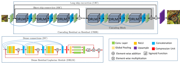
In this section, we provide more details on the cascading residual on the residual structure, which has a hierarchical architecture and composed of cascading blocks. Each cascading block has a medium skip-connection (MSC), cascading features concatenation and is made up of dense residual Laplacian modules (DRLM) each of which consists of a densely connected residual unit, compression unit and Laplacian pyramid attention unit. The lower part of Figure 2 shows DRLM, which will be explained further in Section 3.3.

Recently, in image recognition [32] and super-resolution [7], residual blocks are stacked together to construct a network of more than 1000 layers and 400 layers, respectively, via skip-connections, although the performance has increased; however, the computational overhead has also increased. We aim here to construct a compact and efficient model with a much lower number of the convolutional layers amidst improved performance and computation time. Therefore, we introduce cascading of the blocks employing medium and long skip connections. Let’s suppose that the $n$-th dense residual Laplacian module (DRLM) of the $m$-th cascaded block $B^{n,m}$ is given as:

$$f_{n,m}=f([Z^{u-0;m},Z^{u-1;m},B^{u;m}(w^{u,1;m}),b^{u,1;m})$$ (6)

where $f_{n,m}$ are the features from the $n$-th dense residual Laplacian module (DRLM) of the $m$-th cascaded block. Each cascaded block is composed of $k$ DRLMs, and hence the input to the cascaded block is summed with the output of the $k$ DRLM as $f_{n+k,m}=f_{n+k,m}+f_{n,m}$, i.e. medium skip-connection (MSC) as:

$$f_{g}=f_{0}+H_{crir}(\mathcal{W}_{w,b}),$$ (7)

where $\mathcal{W}_{w,b}$ are the weights and biases learned in the cascaded block. The addition of medium skip-connection eases the flow of information across group of DRLM while the addition of long-skip connection (LSC) helps the flow of information through cascaded blocks. The group features $f_{g}$ are passed to the reconstruction layer to output the same number of channels as the input to the network. Next, we provide information about the dense residual Laplacian modules and its subcomponents.

3.3 Dense Residual Laplacian Module

As briefly mentioned earlier, DRLM is composed of three subcomponents i.e. densely connected residual blocks unit, compression unit, and Laplacian pyramid attention.

The residual blocks we employ, have the traditional two convolutional layers and two ReLUs structure followed by an addition from the input of the residual block, as:

$$R_{i}(w_{i},b_{i})=\tau(f(\tau(f(w_{i,1},b_{i,1});b_{i,2})+Z_{i-1}),$$ (8)

where $Z_{i-1}$ is the output of the previous convolutional layer or residual block while $w_{i,j}$ are the weights of the convolutional layer and $b_{i,j}$ are the biases ($j\in\{1,2\}$). Each densely connected residual unit has three residual blocks with dense connection as

$$\begin{split}R_{c}&=[R_{i-1}(w_{i-1},b_{i-1});R_{i-2}(w_{i-2},b_{i-2})],\\ f_{R}&=R_{i}(w_{i},b_{i})=\tau(f(\tau(f(R_{c}))+R_{c}),\end{split}$$ (9)

where $R_{c}$ is the concatenation of the previous residual blocks and $f_{R}$ is the final output of the densely connected residual unit. The $f_{R}$ features are then passed through a compression unit which compresses the high number of parameters resulted from dense concatenation. The compression unit is comprised of a single convolutional layer with a kernel of 1$\times$1. The compressed features $f_{c}$ are then forwarded to the Laplacian attention unit which is described next.

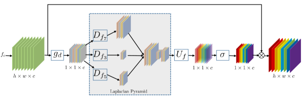
Laplacian Attention: Image Attention has been employed in image classification [41], image captioning [42] etc. to converge on essential image regions. In super-resolution, the same concept with a little variation can be applied that features should be weighted according to their relative importance. Here, we propose Laplacian attention to boost and exploit the relationship between the features that are essential for super-resolving the images.

To produce attention differently at the Laplacian pyramids in the DRLM, we use a global descriptor to capture the statistics expressing the entire image. The proposed Laplacian pyramid weights the sub-band features of high importance progressively in each DRLM. The global descriptor takes the output from the compression unit i.e. $f_{c}$ which has size $h\times w$ with $c$ feature maps. After processing, the global descriptor reduces the size from $h\times w\times c$ to $1\times 1\times c$ as:

Figure 4: Parameters vs. performance. Comparisons are presented on the MANGA109 [43] for 4$\times$ super-resolution.

$$g_{d}=\frac{1}{h\times w}\sum_{i=1}^{h}\sum_{i=1}^{w}f_{c}(i,j),$$ (10)

where $f_{c}(i,j)$ is the value at position $(i,j)$ in the feature maps.

To capture the channel dependencies from the retrieved global descriptor, we utilize a gating approach. As studied in [44], the system must be able to learn the nonlinear synergies between feature maps and mutually-exclusive associations via gating. To implement the gating mechanism formally, we utilize ReLU and sigmoid functions, denoted by $\tau$, and $\sigma$, respectively. The $g_{d}$ features are passed through the Laplacian pyramid to learn the critical features at different scales as:

$$\begin{split}r_{3}&=\tau(D_{f_{3}}(g_{d})),\\ r_{5}&=\tau(D_{f_{5}}(g_{d})),\\ r_{7}&=\tau(D_{f_{7}}(g_{d})),\\ \end{split}$$ (11)

where $D\_$ is the feature reduction operator while the $f_{3},f_{5}$ and $f_{7}$ are the convolutional layers with kernel dilation specified by the subscripts. The multi-level representations $r_{3},r_{5}$ and $r_{7}$ obtained from the the global descriptor $g_{d}$ are concatenated as:

$$g_{p}=[r_{3};r_{5};r_{7}].\\$$ (12)

Furthermore, as shown in Eq 11, the output of the Laplacian pyramid is convolved with a downsampling operator. Therefore, to upsample and differentiate between the features maps, the output is then fed into the upsampling operator $U_{f}$ followed by sigmoid activation as:

$$L_{p}=\sigma(U_{f}(g_{p})).$$ (13)

As a final step, the learned statistics are utilized by adaptively rescaling the output of sigmoid function i.e. $L_{p}$ by the input $f_{c}$ of the Laplacian attention unit as:

$$\hat{f}_{c}=L_{p}\times f_{c}\vspace*{-5mm}$$ (14)

TABLE I: Contribution of different components. Investigation of the performance due to different components of our network.

Dense Connections (DC)		✓				✓	✓	✓	✓	✓
Medium Skip Connections (MSC)		✓	✓	✓	✓				✓	✓
Long Skip Connection (LSC)		✓	✓	✓		✓	✓			✓
Laplacian Attention (LA)				✓			✓			✓
PSNR (in dB)	31.92	32.30	32.06	32.06	32.07	31.85	32.12	31.97	32.10	32.37

Figure 5: Performance vs. Time. Comparisons are presented on the URBAN100 [45] for 4$\times$ super-resolution. Our proposed method strides a balance between performance and computation time.

	Original	Bicubic	SRCNN [11]	VDSR [9]	MSLapSRN [6]
	PSNR/SSIM	21.58/0.6290	22.03/0.6786	22.15/0.6925	22.31/0.7030
Urban100 (4$\times$)	DRRN [12]	EDSR [5]	RCAN [7]	CARN [8]	Ours
img$\_$076	21.93/0.6903	23.07/0.7367	24.31/0.7897	22.57/0.7175	24.62/0.8032
	Original	Bicubic	SRCNN [11]	VDSR [9]	MSLapSRN [6]
	PSNR/SSIM	26.92/0.7254	29.70/0.8102	29.69/0.8312	30.03/0.8430
Urban100 (4$\times$)	DRRN [12]	EDSR [5]	RCAN [7]	CARN [8]	Ours
img$\_$044	29.30/0.8373	33.36/0.9054	31.45/0.7955	31.34/0.8648	34.77/0.9188
	Original	Bicubic	SRCNN [11]	FSRCNN [20]	LapSRN [10]
	PSNR/SSIM	24.69/0.7873	26.26/0.8487	26.38/0.8500	26.92/0.8752
MANGA109 (4$\times$)	VDSR [9]	DRRN [12]	RCAN [7]	CARN [8]	Ours
YumeiroCooking	26.92/0.8731	27.20/0.8822	29.85/0.9368	27.58/0.8953	30.33/0.9422

Figure 6: Visual comparison for 4$\times$. Super-resolution comparison on sample images with sharp edges and texture, taken from URBAN100 [45] and MANGA109 [43] for the scale of 4$\times$. The sharpness of the edges on the objects and textures restored by our method is the best.

3.4 Implementation

In this section of the paper, we present the implementation details of our system. In each cascading residual on the residual block, we have three ($k$=3) DRLMs, and in each DRLM, we have three RBs densely connected, one compression unit and one Laplacian attention. The filter size in all the layers is set to 3$\times$3 with dilation of 1$\times$1 except in the Laplacian pyramid where it is three, five and seven. Likewise, the number of feature maps in all the convolutional layers are fixed to 64, except the last reconstruction layer where the output is either one for grayscale or three for color images. To keep the size of the feature maps the same, zeros are padded accordingly. In pyramid attention, the feature maps are reduced by a factor of four. We also use a post-upscaling procedure instead of pre-scaling for more efficient processing and to avoid the pre-scaling artifacts.

4 Experiments

In this section, we first examine the contributions of various elements of our proposed network. Then we test the model on five publicly available super-resolution dataset, namely, SET5 [46], SET14 [47], URBAN100 [45], B100 [48], and MANGA109 [43]. The metrics employed for evaluation are PSNR and SSIM on the luminance channel obtained through YCbCr color space. We also give a comparison on object recognition performance against the competing super-resolution methods.

4.1 Training settings

To make fair comparisons with the current state-of-the-art use CNN methods [35, 7, 5], we use the same settings which are specified in their particular papers. Similar to [35], we train our network on DIV2K and Flicker2K datasets [49]. Furthermore, we diversify the training images through data augmentation, which is accomplished by random rotations using multiples of 90$\degree$ supplemented via horizontal and vertical flipping. The batch size is 16 while the size of the low-resolution input is $48\times 48$. To optimize the system, ADAM [50] is utilized with the default parameters of $\beta_{1}$ =0.9, $\beta_{2}$ =0.999, and $\epsilon=10^{-8}$. The learning rate is fixed to $10^{-4}$ originally and then decreased to half after every $2\times 10^{5}$ iterations. The network is designed utilizing the PyTorch framework [51] on a Tesla P100 GPU.

4.2 Ablation Studies

4.2.1 Influence of the skip connections

Skip connections are the backbone of the current state of the art network [9, 8, 15, 7]. Here, we demonstrate the effectiveness of the skip-connections i.e. Long skip connection (LSC), Medium skip connection (MSC), and dense local connections (DLC), in our model. The connections are categorized based on their length. Table I shows the average PSNR on SET5 for 2$\times$ for the different settings of connections. The PSNR is higher when all the connections are present while the performance relatively downgrades when some of the connections are absent. In the absence of all connections, the depth of the network does not yield benefit. This experiment illustrates the significance of the different connection types for our deep network.

	Original	Bicubic	SRCNN [11]	FSRCNN [20]	VDSR [9]
	PSNR/SSIM	18.41/0.3189	18.79/0.3416	19.01/0.3519	19.10/0.3578
Urban100 (8$\times$)	DRCN [13]	DRRN [12]	MSLapSRN [6]	RCAN [7]	Ours
img$\_$045	19.18/0.3728	19.76/0.4043	18.87/0.3819	19.93/0.4035	20.58/0.4549
	Original	Bicubic	SRCNN [11]	FSRCNN [20]	VDSR [9]
	PSNR/SSIM	24.91/0.7578	25.97/0.7894	26.07/0.7766	26.37/0.7981
MANGA109 [43] (8$\times$)	DRCN [13]	DRRN [12]	MSLapSRN [6]	RCAN [7]	Ours
TaiyouNiSmash	27.09/0.8216	27.60/0.8378	28.02/0.8532	30.68/0.8962	31.09/0.9032

Figure 7: Visual comparison for 8$\times$. Comparisons on images with fine details for a high upsampling factor of 8$\times$ on URBAN100 [45] and MANGA109 [43]. The best results are in bold.

4.2.2 Laplacian attention

The second essential component of our model is Laplacian attention. We provide a comparison of the network with and without the use of Laplacian attention in Table I. The results shown support our claim that the selection of essential features through multiple frequency bands assist enhancement of the image and improve the overall accuracy. It should be considered that super-resolution techniques [5, 18] have matured greatly since SRCNN [28] and further improvement requires sophisticated network design and the weighting of features through appropriate selection criteria. Both of the mentioned provisions are achieved in our model through Laplacian pyramid attention, and cascading with residual on the residual architecture.

4.2.3 Parameters, runtime, and depth analysis

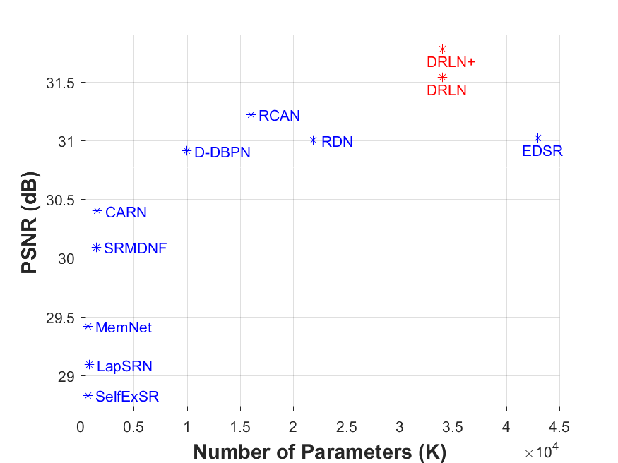
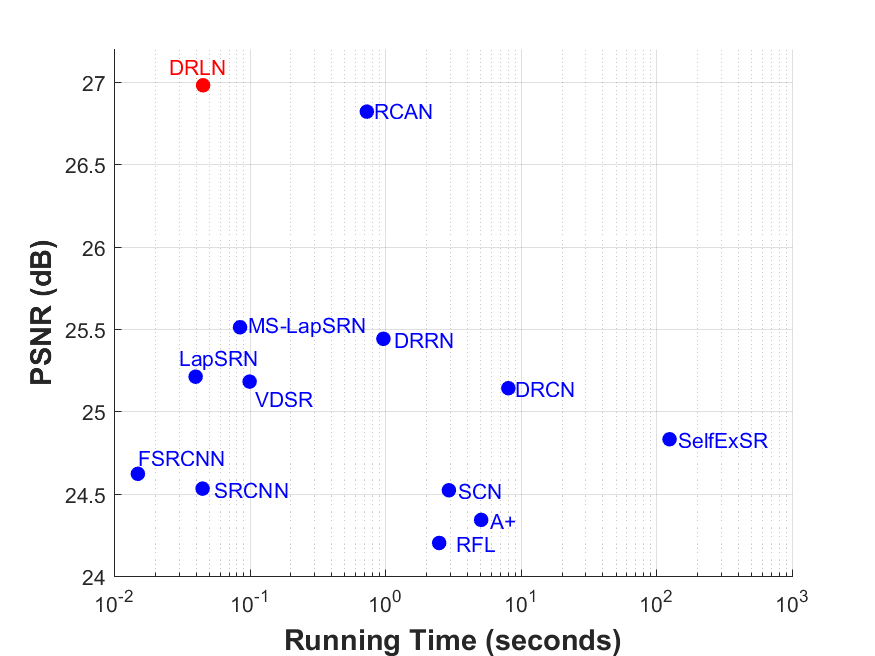
The number of parameters is a crucial factor in determining the potential of the CNN networks. More parameters usually lead to better performance, however, computing more parameters requires deeper networks, which increases the computational load. Our aim here is to utilize previously computed features; hence, concatenating the earlier computed features maps strike a balance between performance, depth, and run time. Furthermore, our network achieves state-of-the-art performance with a mere 160 convolutional layers as compared to RCAN [7] i.e. 400+. In Figure 4, we provide a comparison of the parameters and the performance. Our model has fewer parameters as compared to EDSR [5] and the runtime is less as compared to RCAN [7] i.e. the time taken by RCAN for an image of size 824$\times$1168 on average is 1.14s opposed to our method 0.045s on MANGA109 [45] for 4$\times$. This efficiency is due to the fact that our method mainly uses concatenations instead of expensive addition operations. In Figure 5, the runtime comparisons are provided against state-of-the-art methods. The PSNR and efficiency are higher for our model, which essentially demonstrates that compact models can push the boundaries with non-conventional architectures.

4.3 Comparisons

We present the comparison of our model with the state-of-the-art CNN models which include SRCNN [28], FSRCNN [20], VDSR [9], SCN [52], SPMSR [53], LapSRN [10], MSLapSRN [6], MemNet [23], EDSR [5], SRMDNF [22], D-DBPN [18], IRCNN [21], RDN [15], RCAN [7] and CARN [8]. Similar to [5], we employ self-ensemble to boost the performance of our model and denote it with a ’+’ to differentiate it from the single model.

Similar to contemporary state-of-the-art models, we experiment on two types of image degradations; bicubic-downsample and blur-downsample [21]. For evaluation of the models, the bicubic downsampling scales of 2$\times$, 3$\times$, 4$\times$, and 8$\times$ are adopted, while blur-downsampling is achieved through a Gaussian kernel having 1.6$\sigma^{2}$ for a scale of 3$\times$.

TABLE II: Quantitative evaluation of competing methods. We report the performance of state-of-the-art algorithms on widely used publicly available datasets, in terms of PSNR (in dB) and SSIM. The best results are highlighted with red color while the blue color represents the second best SR.

Method	Scale	SET5 [46]		SET14 [47]		BSD100 [48]		URBAN100 [45]		MANGA109 [43]
		PSNR	SSIM	PSNR	SSIM	PSNR	SSIM	PSNR	SSIM	PSNR	SSIM
Bicubic		33.66	0.9299	30.24	0.8688	29.56	0.8431	26.88	0.8403	30.80	0.9339
SRCNN [11]		36.66	0.9542	32.45	0.9067	31.36	0.8879	29.50	0.8946	35.60	0.9663
FSRCNN [20]		37.05	0.9560	32.66	0.9090	31.53	0.8920	29.88	0.9020	36.67	0.9710
VDSR [9]		37.53	0.9590	33.05	0.9130	31.90	0.8960	30.77	0.9140	37.22	0.9750
LapSRN [10]		37.52	0.9591	33.08	0.9130	31.08	0.8950	30.41	0.9101	37.27	0.9740
MemNet [23]		37.78	0.9597	33.28	0.9142	32.08	0.8978	31.31	0.9195	37.72	0.9740
EDSR [5]		38.11	0.9602	33.92	0.9195	32.32	0.9013	32.93	0.9351	39.10	0.9773
SRMDNF [22]	2$\times$	37.79	0.9601	33.32	0.9159	32.05	0.8985	31.33	0.9204	38.07	0.9761
D-DBPN [18]		38.09	0.9600	33.85	0.9190	32.27	0.9000	32.55	0.9324	38.89	0.9775
RDN [15]		38.24	0.9614	34.01	0.9212	32.34	0.9017	32.89	0.9353	39.18	0.9780
RCAN [7]		38.27	0.9614	34.12	0.9216	32.41	0.9027	33.34	0.9384	39.44	0.9786
CARN [8]		37.76	0.9590	33.52	0.9166	32.09	0.8978	31.92	0.9256	38.36	0.9764
DRLN (ours)		38.27	0.9616	34.28	0.9231	32.44	0.9028	33.37	0.9390	39.58	0.9786
DRLN+ (ours)		38.34	0.9619	34.43	0.9247	32.47	0.9032	33.54	0.9402	39.75	0.9792
Bicubic		30.39	0.8682	27.55	0.7742	27.21	0.7385	24.46	0.7349	26.95	0.8556
SRCNN [11]		32.75	0.9090	29.30	0.8215	28.41	0.7863	26.24	0.7989	30.48	0.9117
FSRCNN [20]		33.18	0.9140	29.37	0.8240	28.53	0.7910	26.43	0.8080	31.10	0.9210
VDSR [9]		33.67	0.9210	29.78	0.8320	28.83	0.7990	27.14	0.8290	32.01	0.9340
LapSRN [10]		33.82	0.9227	29.87	0.8320	28.82	0.7980	27.07	0.8280	32.21	0.9350
MemNet [23]		34.09	0.9248	30.00	0.8350	28.96	0.8001	27.56	0.8376	32.51	0.9369
EDSR [5]	3$\times$	34.65	0.9280	30.52	0.8462	29.25	0.8093	28.80	0.8653	34.17	0.9476
SRMDNF [22]		34.12	0.9254	30.04	0.8382	28.97	0.8025	27.57	0.8398	33.00	0.9403
RDN [15]		34.71	0.9296	30.57	0.8468	29.26	0.8093	28.80	0.8653	34.13	0.9484
RCAN [7]		34.74	0.9299	30.65	0.8482	29.32	0.8111	29.09	0.8702	34.44	0.9499
CARN [8]		34.29	0.9255	30.29	0.8407	29.06	0.8034	28.06	0.8493	33.49	0.9440
DRLN (ours)		34.78	0.9303	30.73	0.8488	29.36	0.8117	29.21	0.8722	34.71	0.9509
DRLN+ (ours)		34.86	0.9307	30.80	0.8498	29.40	0.8125	29.37	0.8746	34.94	0.9518
Bicubic		28.42	0.8104	26.00	0.7027	25.96	0.6675	23.14	0.6577	24.89	0.7866
SRCNN [11]		30.48	0.8628	27.50	0.7513	26.90	0.7101	24.52	0.7221	27.58	0.8555
FSRCNN [20]		30.72	0.8660	27.61	0.7550	26.98	0.7150	24.62	0.7280	27.90	0.8610
VDSR [9]		31.35	0.8830	28.02	0.7680	27.29	0.0726	25.18	0.7540	28.83	0.8870
LapSRN [10]		31.54	0.8850	28.19	0.7720	27.32	0.7270	25.21	0.7560	29.09	0.8900
MemNet [23]		31.74	0.8893	28.26	0.7723	27.40	0.7281	25.50	0.7630	29.42	0.8942
EDSR [5]		32.46	0.8968	28.80	0.7876	27.71	0.7420	26.64	0.8033	31.02	0.9148
SRMDNF [22]	4$\times$	31.96	0.8925	28.35	0.7787	27.49	0.7337	25.68	0.7731	30.09	0.9024
D-DBPN [18]		32.47	0.8980	28.82	0.7860	27.72	0.7400	26.38	0.7946	30.91	0.9137
RDN [15]		32.47	0.8990	28.81	0.7871	27.72	0.7419	26.61	0.8028	31.00	0.9151
RCAN [7]		32.63	0.9002	28.87	0.7889	27.77	0.7436	26.82	0.8087	31.22	0.9173
CARN [8]		32.13	0.8937	28.60	0.7806	27.58	0.7349	26.07	0.7837	30.40	0.9082
DRLN (ours)		32.63	0.9002	28.94	0.7900	27.83	0.7444	26.98	0.8119	31.54	0.9196
DRLN+ (ours)		32.74	0.9013	29.02	0.7914	27.87	0.7453	27.14	0.8149	31.78	0.9211
Bicubic		24.40	0.6580	23.10	0.5660	23.67	0.5480	20.74	0.5160	21.47	0.6500
SRCNN [11]		25.33	0.6900	23.76	0.5910	24.13	0.5660	21.29	0.5440	22.46	0.6950
FSRCNN [20]		20.13	0.5520	19.75	0.4820	24.21	0.5680	21.32	0.5380	22.39	0.6730
SCN [52]		25.59	0.7071	24.02	0.6028	24.30	0.5698	21.52	0.5571	22.68	0.6963
VDSR [9]		25.93	0.7240	24.26	0.6140	24.49	0.5830	21.70	0.5710	23.16	0.7250
LapSRN [10]		26.15	0.7380	24.35	0.6200	24.54	0.5860	21.81	0.5810	23.39	0.7350
MemNet [23]	8$\times$	26.16	0.7414	24.38	0.6199	24.58	0.5842	21.89	0.5825	23.56	0.7387
MSLapSRN [6]		26.34	0.7558	24.57	0.6273	24.65	0.5895	22.06	0.5963	23.90	0.7564
EDSR [5]		26.96	0.7762	24.91	0.6420	24.81	0.5985	22.51	0.6221	24.69	0.7841
D-DBPN [18]		27.21	0.7840	25.13	0.6480	24.88	0.6010	22.73	0.6312	25.14	0.7987
RCAN [7]		27.31	0.7878	25.23	0.6511	24.98	0.6058	23.00	0.6452	25.24	0.8029
DRLN (ours)		27.36	0.7882	25.34	0.6531	25.01	0.6057	23.06	0.6471	25.29	0.8041
DRLN+ (ours)		27.46	0.7916	25.40	0.6547	25.06	0.6070	23.24	0.6523	25.55	0.8087

4.3.1 Bicubic degradations

In this section, we provide the qualitative results of our model against competitive methods in Figure 6 and 7.

4$\times$ Visual Comparisons: To be fair in comparison, the images furnished for qualitative comparison in Figure 6 are from the same dataset images as RCAN [7]. The first two images are from URBAN100 [45], and the last picture is from MANGA109 [43] for upscaling of 4$\times$. As shown in Figure 6, all competing methods, in general, fail to recover edges and introduce blurring artifacts. In “img_076”, the competing CNN algorithms are unable to retrieve the rectangular shapes and blur out the edges and boundaries representing the outlines of the windows. Our method is faithful to the original image, providing results with proper rectangular structures and straight lines.

Similarly, in the second example, i.e. “img_044” in Figure 6, most of the methods distort the horizontal lines and blur out the background. Furthermore, the orientation of the lines on the cropped parts is in the opposite direction and forms a checkerboard pattern for [11, 9]. Moreover, a close inspection reveals that RCAN [7] and CARN [8] fused the background with the horizontal lines, removing the sharpness from the images shown while in our case, the lines are clearly visible and separated from the background, recovering sharp details.

The last image in Figure 6 is from MANGA109 [43] for 4$\times$ scale. The textures in the cropped regions are blemished and mixed by together most of the state-of-the-art methods and are unable to recover the shape of the green colored strokes except for RCAN [7]. However, RCAN [7] is also unequipped to super-resolve the lines correctly as it can be witnessed that the lines are blended in the right side of the cropped image. Furthermore, the super-resolved green lines are blurry in the case of RCAN [7]. Our network can super-resolve most of the details and textures without producing visible artifacts from the shown low-resolution image. The green lines are sharp and closer in structure to the original.

	Original	Bicubic	SRCNN [11]	FSRCNN [20]	VDSR [9]
	PSNR/SSIM	26.10/0.7032	27.91/0.7874	24.34/0.6711	28.34/0.8166
URBAN100 (3$\times$)	IRCNN [21]	SRMDNF [22]	RDN [15]	RCAN [7]	Ours
img_078	28.57/0.8184	29.08/0.8342	29.94/0.8513	30.65/0.8624	31.13/0.8685
	Original	Bicubic	FSRCNN [20]	VDSR [9]	IRCNN [21]
	PSNR/SSIM	22.58/0.84597	21.09/0.8254	19.30/0.6960	24.60/0.9092
URBAN100 (3$\times$)	EDSR [5]	SRMDNF [22]	RCAN [7]	CARN [8]	Ours
img_062	24.48/0.9105	28.63/0.9695	29.41/0.9775	24.45/0.9096	30.78/0.9830

Figure 8: Blur-Downscale (BD) degradation. Comparison on sample images with sharp edges and texture, taken from URBAN100 and SET14 datasets for the scale of 3$\times$. The sharpness of the edges on the objects and textures restored by our method is the best.

TABLE III: Quantitative results with blur-down degradation. The best results are highlighted with red color while the blue color represents the second best.

		SET5 [46]		SET14 [47]		BSD100 [48]		URBAN100 [45]		MANGA109 [43]
Method	Scale	PSNR	SSIM	PSNR	SSIM	PSNR	SSIM	PSNR	SSIM	PSNR	SSIM
Bicubic		28.78	0.8308	26.38	0.7271	26.33	0.6918	23.52	0.6862	25.46	0.8149
SPMSR		32.21	0.9001	28.89	0.8105	28.13	0.7740	25.84	0.7856	29.64	0.9003
SRCNN [11]		32.05	0.8944	28.80	0.8074	28.13	0.7736	25.70	0.7770	29.47	0.8924
FSRCNN [20]		26.23	0.8124	24.44	0.7106	24.86	0.6832	22.04	0.6745	23.04	0.7927
VDSR [9]		33.25	0.9150	29.46	0.8244	28.57	0.7893	26.61	0.8136	31.06	0.9234
IRCNN [21]	3$\times$	33.38	0.9182	29.63	0.8281	28.65	0.7922	26.77	0.8154	31.15	0.9245
SRMDNF [22]		34.01	0.9242	30.11	0.8364	28.98	0.8009	27.50	0.8370	32.97	0.9391
RDN [15]		34.58	0.9280	30.53	0.8447	29.23	0.8079	28.46	0.8582	33.97	0.9465
RCAN [7]		34.70	0.9288	30.63	0.8462	29.32	0.8093	28.81	0.8647	34.38	0.9483
DRLN (ours)		34.81	0.9297	30.81	0.8487	29.40	0.8121	29.11	0.8697	34.84	0.9506
DRLN+ (ours)		34.87	0.9301	30.86	0.8495	29.44	0.8128	29.26	0.8718	35.07	0.9516

8$\times$ Visual Comparisons: To show the powerful reconstruction ability of our network, we present extreme examples of 8$\times$ super-resolution in Figure 7 from URBAN100 [45] and MANGA109 [43]. Because of the significant scaling factor in image “img_045”, the models [28, 9, 13] using bicubic upsampled input creates artificial checkerboard artifacts and structures in the images due to the incorrect initial input. While, on the other hand, the recent state-of-the-art method [7] which takes the low-resolution photographs as input, is unable to recover the high frequencies reliably due to the notable upscaling and also produces new structures instead of recovering the original lines. MSLapSRN [6] is able to super-resolve the lines correctly in the lower half of the image, and this may be due to the progressive reconstruction i.e. employing loss after every 2$\times$ resolution to achieve 8$\times$ output. In our case, the lines are super-resolved correctly without employing multiple losses. This shows the super-resolution capability of our CNN model.

Original(PSNR/SSIM)		IRCNN [21] (28.73/0.6762)		RCAN [7] (28.44/0.6607)		Ours (32.46/0.8760)

Figure 9: Noisy SR visual Comparison on BSD100. Textures on the birds are much better reconstructed, and the noise removed by our method as compared to the IRCNN [21] and RCAN [7] for $\sigma=10$.

Noisy	GT	BM3D-SR [54]	BM3D-SRNI [55]	Ours
$\sigma=20$	PSNR/SSIM	25.05/0.5868	25.31/0.6206	27.03/0.7330

Figure 10: Noisy visual comparison on Llama. Textures on the fur, and on rocks in the background are much better reconstructed in our result as compared to the conventional BM3D-SR and BM3D-SRNI.

The second low-resolution image, in Figure 7 for 8$\times$ is from MANGA109 [43], titled, “TaiyouNiSmash”, contains minimal high-frequencies and hence is challenging to super-resolve to the desired outcome. Nevertheless, our method still can reproduce better results and avoids producing blurring and artificial structures as compared to competitive techniques. The algorithms of VDSR [9], MSLapSRN [6], etc. creates blurry outputs and unsharp images. Similarly, RCAN [7] can produce slightly sharp edges than its predecessor; however, it connected the gaps in different letters. Our model is more faithful to the original image and better captures the small gaps present in the letters.

Quantitative Comparisons: Table II shows the quantitative results for all the competing methods. These results are borrowed from their corresponding published papers. Our scheme outperforms all other approaches on all datasets for all scales which complements the visual sequences presented earlier in Figures 6 and 7. Our model quantitative results outperform even without employing the self-ensemble technique.

The improvement of our method on SET5 [46] and SET14 [47] is marginal due to a small number of images (the number with the dataset shows the images present i.e. SET5 has only five photographs, and SET14 has only 14 images) in these mentioned datasets; however, a clear trend emerges when the number of images increases. For example, on MANGA109 [43], the average PSNR increment across all scales for our model is 0.34dB and 3.98dB compared to second leading method i.e. RCAN [7] and the pioneering SRCNN [28], respectively.

Figure 11: Noisy super-resolution. The plots show average PSNR as functions of noise sigma. Our method consistently improves over specific noisy super-resolution methods and CNN for all $\sigma$ levels.

4.3.2 Blur-Downscale (BD) degradations

More recently, blur-down (BD) degraded images [21] are super-resolved to showcase the potential of super-resolution architectures. We also utilize blur-downsampled photographs to compare against the state-of-the-art.

3$\times$ Visual Comparisons: We first present three examples; two from URBAN100 [45] and one from MANGA109 [43] in Fig. 8. The images from URBAN100 [45] super-resolved by the competing methods contain blur effects near the upper end of the buildings as can be seen in the cropped versions. The only methods which perform comparatively better are RDN [15] and RCAN [7]; however, our approach is not only able to remove the blur but also restore the high-frequency details. This may be due to the Laplacian-attention used at the end of each DRLM, which captures the important discriminative features that are useful for high-frequency restoration.

Next, we evaluate our algorithm on an image from the classical SET14 [47] shown in Figure 8. In the crop sections, our method produces relatively sharp edges and crisper text than state-of-the-art algorithms which mostly exhibit blurry and distorted text. IRCNN [21], SRMD [22], and RCAN [7] are specifically designed to handle blur-downscale super-resolution; however, our method produces best qualitative results having more than 1dB PSNR for this particular image.

Quantitative Comparisons: Next, Table III provides the comparison against nine competitive methods. Here, again RDN [15] and RCAN [7] shows good results compared to [28, 21, 9]; however, our single and self-ensemble models achieve a notable performance gain over all methods in general, and RDN [15] and RCAN [7] particular. The average PSNR gain over both the mentioned methods for 3$\times$ super-resolution of blur-down degraded images is 0.55dB and 0.33dB for all the datasets. Our architecture better generalizes the task at hand, and our Laplacian attention can select the relevant features more reliably in contrast to RCAN’s [7] channel attention.

TABLE IV: Objection recognition. We report the performance of ResNet [4] using different SR algorithms as a pre-processing step.

Evaluation	Bicubic	DRCN [13]	FSRCNN [20]	PSyCo [57]	ENet-E [33]	RCAN [7]	Ours	Baseline
Top-1 error	0.506	0.477	0.437	0.454	0.449	0.393	0.345	0.260
Top-5 error	0.266	0.242	0.196	0.224	0.214	0.167	0.121	0.072

4.3.3 Noisy downscale (ND) degradations

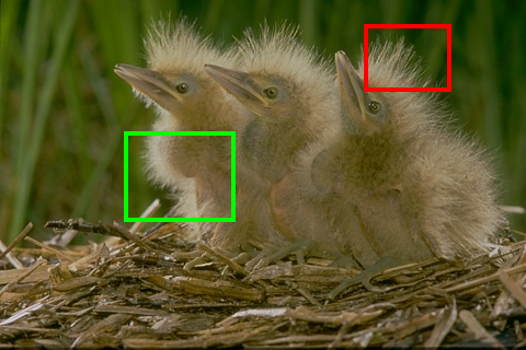
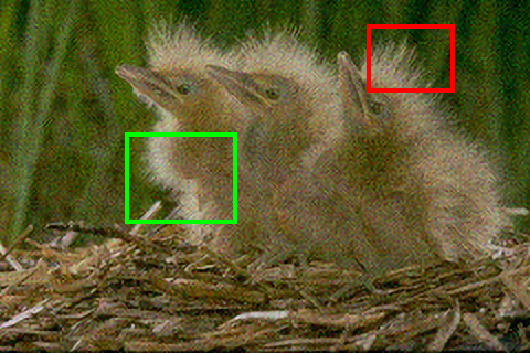
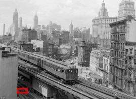
2$\times$ Visual Comparisons: We present two images for super-resolving the noisy images. Figure 10 shows the comparison of our method with CNN methods on the Birds image from BSD100 [48] for a low-level noise ($\sigma=10$). It can be observed that our method significantly recovered more texture and removed the noise close to the ground truth image. IRCNN [21] and RCAN [7] fail to remove the noise, rather they amplify it. The other noisy image, “Llama”, shown in Figure 10 is taken from Singh et al. [55] for a fair comparison against traditional algorithms. The difference in texture details on the fur and the background can be observed in our case and the conventional methods. Our method can super-resolve the fur more appropriately as compared to the other methods.

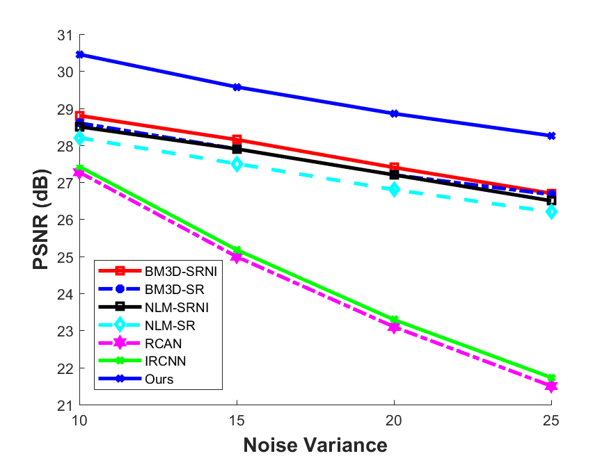
Quantitative Comparisons: To compare quantitatively, we follow the footsteps of Singh et al. [55] which uses the first 50 images from the BSD100 [48]. We compare against super-resolving noisy image algorithms, which include (SRNI) [55], BM3D-SR [54] and NLM-SR [56] as well as the image restoration algorithm IRCNN [21]. Moreover, BM3D-SR or NLM-SR indicates applying the traditional denoising approach first i.e. (BM3D or NLM), followed by image super-resolution (SR).

Currently, RCAN [7] is state-of-the-art in single image super-resolution; however, we show that it is unable to handle noisy images. In Figure 11, we present the quantitative results with the competing algorithms for four noise levels i.e. $\sigma~{}=~{}10,15,20$ and $25$. Our algorithm constantly outperforms CNN-based algorithms and specifically designed methods at all noise levels. Furthermore, the CNN methods [21, 7] performance is relative to the traditional algorithms when the noise levels are low i.e. $\sigma~{}=~{}10$ and $15$; however, it degrades significantly as $\sigma$ increases while, on the other hand, the performance of our algorithm is better at high-noise levels as well.

	Bicubic	SRCNN [11]
LR input	DRCN [13]	Ours
	FSRCNN [20]	VDSR [9]
LR input	MSLapSRN [6]	Ours

Figure 12: Comparison of real-world images. In these cases, neither the downsampling blur kernels nor the ground-truth images are available. In the top photograph, our methods reconstruct the letters “W” and “I” correctly while the competing methods combine the letters. Similarly, in the bottom picture, the rail is accurately super-resolved without any artifacts while others fail to super-resolve the horizontal lines correctly.

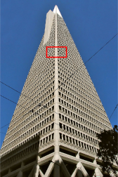
4.3.4 Real-World historic super-resolution

In this section, we illustrate the application of our algorithm on real-world historic [10] images suffering from JPEG compression artifacts. The information about the downsampling operators and ground-truth images are unavailable. The results of our reconstruction against state-of-the-art algorithms are shown in Figure 12. The output of our algorithm is clear and sharper as shown in both Figures.

4.4 Performance on Object Recognition

As discussed earlier, image restoration tasks assist in high-level computer vision tasks; therefore, we demonstrate and analyze the effectiveness of our method on object recognition current state-of-the-art super-resolution techniques. We use the same settings as [7], which evaluates the performance on the initial 1k images from ImageNet [58]. The image of size 224$\times$224 is downscaled by 4$\times$ to achieve the image size of 56$\times$56. The downscaled versions are then upscaled to the original size images via the super-resolution algorithms and subsequently fed through ResNet50 [32] for classifications. The accuracy of the classification network is used to determine the potential of the super-resolution algorithms.

We compare with six methods i.e. Bicubic, DRCN [13], FSRCNN [20], PSyCo [57], ENet-E [33] and RCAN [7]. The top-1 and top-5 errors for object recognition are recorded in Table IV. Our method is more accurate as it provides the lowest error; hence, this illustrates the ability of our network to reconstruct appropriate frequencies more reliably.

4.5 Limitations

	GT	Bicubic	SRCNN [11]
	FSRCNN [20]	SelfExSR [59]	DRCN [13]
Ground-truth	VDSR [9]	LapSRN [10]	Ours

Figure 13: Limitation. A failure case for super-resolution of 8$\times$. Our algorithm is not able to create finer details if the input low-resolution images lack sufficient high-frequency details.

Our model has shown the ability to render sharp and clean images for all upsampling scales; however, it struggles to “hallucinate” finer details. For example, an image with 8$\times$ is shown in Figure 13, the top of the building is very challenging as due to the large downsampling operator i.e. 8$\times$. All the algorithms fail to recover the fine details at this level. The traditional methods, e.g. SelfExSR [59], which exploit the self-similarity and 3D scene geometry, also fail to recover fine details. Similarly, MS-LapSRN [6] progressively upsamples to produce the 8$\times$ results as opposed to ours where the 8$\times$ upsampling is achieved directly; however, [6] is unable to give the desired outcome. Furthermore, this limitation is common to all the super-resolution methods [6, 7, 11, 9].

5 Conclusion

In this exposition, we propose a modular convolution neural network for highly accurate image super-resolution. We also employ various components to boost the performance of super-resolution. We thoroughly analyze and present a comprehensive evaluation of the choice of our network design.

We employ cascading residual on the residual structure to design a large depth network using long skip connection, short skip connection, and local connections. The cascading residual on the residual architecture helps in the flow of low-frequency information to make network learn high and mid-level frequency information. We use densely connected residual blocks, which re-use the previously computed features. This type of setting has multiple advantages such as implicit “deep supervision” and learning from high-level complex features. We also introduce Laplacian attention, which models the essential features on multiple scales and learns the inter and intra-level dependencies between the feature maps.

Furthermore, we perform an extensive evaluation of super-resolution datasets, low-resolution noisy images and real-world images (unknown blur downsampling). We also have shown the results on Bicubic and blur-down kernels to demonstrate the effectiveness of our proposed methods. Further, we present the performance of object recognition on the super-resolved images by different methods. We have illustrated the potential of our network for image super-resolution; however, our network is general and can be applied to other low-level vision tasks such as image restoration, synthesis, and transformation problems.

References

- [1] S. P. Mudunuri and S. Biswas, “Low resolution face recognition across variations in pose and illumination,” TPAMI, 2016.
- [2] H. Greenspan, “Super-resolution in medical imaging,” CJ, 2008.
- [3] A. Swaminathan, M. Wu, and K. R. Liu, “Digital image forensics via intrinsic fingerprints,” TIFS, 2008.
- [4] K. He, X. Zhang, S. Ren, and J. Sun, “Deep residual learning for image recognition,” in CVPR, 2016.
- [5] B. Lim, S. Son, H. Kim, S. Nah, and K. M. Lee, “Enhanced deep residual networks for single image super-resolution,” in CVPRW, 2017.
- [6] W.-S. Lai, J.-B. Huang, N. Ahuja, and M.-H. Yang, “Fast and accurate image super-resolution with deep laplacian pyramid networks,” TPAMI, 2018.
- [7] Y. Zhang, K. Li, K. Li, L. Wang, B. Zhong, and Y. Fu, “Image super-resolution using very deep residual channel attention networks,” ECCV, 2018.
- [8] N. Ahn, B. Kang, and K.-A. Sohn, “Fast, accurate, and, lightweight super-resolution with cascading residual network,” ECCV, 2018.
- [9] J. Kim, J. Kwon Lee, and K. Mu Lee, “Accurate image super-resolution using very deep convolutional networks,” in CVPR, 2016.
- [10] W.-S. Lai, J.-B. Huang, N. Ahuja, and M.-H. Yang, “Deep laplacian pyramid networks for fast and accurate superresolution,” in CVPR, 2017.
- [11] C. Dong, C. C. Loy, K. He, and X. Tang, “Image super-resolution using deep convolutional networks,” TPAMI, 2016.
- [12] Y. Tai, J. Yang, and X. Liu, “Image super-resolution via deep recursive residual network,” in CVPR, 2017.
- [13] J. Kim, J. Kwon Lee, and K. Mu Lee, “Deeply-recursive convolutional network for image super-resolution,” in CVPR, 2016.
- [14] T. Tong, G. Li, X. Liu, and Q. Gao, “Image super-resolution using dense skip connections,” in ICCV, 2017.
- [15] Y. Zhang, Y. Tian, Y. Kong, B. Zhong, and Y. Fu, “Residual dense network for image super-resolution,” in CVPR, 2018.
- [16] C. Ledig, L. Theis, F. Huszár, J. Caballero, A. Cunningham, A. Acosta, A. P. Aitken, A. Tejani, J. Totz, Z. Wang et al., “Photo-realistic single image super-resolution using a generative adversarial network.”
- [17] J.-H. Kim, J.-H. Choi, M. Cheon, and J.-S. Lee, “Ram: Residual attention module for single image super-resolution,” arXiv, 2018.
- [18] M. Haris, G. Shakhnarovich, and N. Ukita, “Deep backprojection networks for super-resolution,” in CVPR, 2018.
- [19] K. He, X. Zhang, S. Ren, and J. Sun, “Delving deep into rectifiers: Surpassing human-level performance on imagenet classification,” in ICCV, 2015.
- [20] C. Dong, C. C. Loy, and X. Tang, “Accelerating the super-resolution convolutional neural network,” in ECCV, 2016.
- [21] K. Zhang, W. Zuo, S. Gu, and L. Zhang, “Learning deep cnn denoiser prior for image restoration,” in CVPR, 2017.
- [22] K. Zhang, W. Zuo, and L. Zhang, “Learning a single convolutional super-resolution network for multiple degradations,” in CVPR, 2018.
- [23] Y. Tai, J. Yang, X. Liu, and C. Xu, “Memnet: A persistent memory network for image restoration,” in CVPR, 2017.
- [24] G. Huang, Z. Liu, L. van der Maaten, and K. Q. Weinberger, “Densely connected convolutional networks,” in CVPR, 2017.
- [25] H. Ren, M. El-Khamy, and J. Lee, “Image super resolution based on fusing multiple convolution neural networks,” in CVPRW, 2017.
- [26] Y. Hu, X. Gao, J. Li, Y. Huang, and H. Wang, “Single image super-resolution via cascaded multi-scale cross network,” arXiv, 2018.
- [27] Z. Hui, X. Wang, and X. Gao, “Fast and accurate single image super-resolution via information distillation network,” in CVPR, 2018.
- [28] C. Dong, C. Loy, K. He, and X. Tang, “Learning a deep convolutional network for image super-resolution,” in ECCV, 2014.
- [29] A. L. Maas, A. Y. Hannun, and A. Y. Ng, “Rectifier nonlinearities improve neural network acoustic models,” in ICML, 2013.
- [30] A. Radford, L. Metz, and S. Chintala, “Unsupervised representation learning with deep convolutional generative adversarial networks,” arXiv, 2015.
- [31] I. Goodfellow, J. Pouget-Abadie, M. Mirza, B. Xu, D. Warde-Farley, S. Ozair, A. Courville, and Y. Bengio, “Generative adversarial nets,” in NIPS, 2014.
- [32] K. He, X. Zhang, S. Ren, and J. Sun, “Deep residual learning for image recognition,” in CVPR, 2016.
- [33] M. S. Sajjadi, B. Schölkopf, and M. Hirsch, “Enhancenet: Single image super-resolution through automated texture synthesis,” in ICCV, 2017.
- [34] S.-J. Park, H. Son, S. Cho, K.-S. Hong, and S. Lee, “Srfeat: Single image super-resolution with feature discrimination,” in ECCV, 2018.
- [35] X. Wang, K. Yu, S. Wu, J. Gu, Y. Liu, C. Dong, C. C. Loy, Y. Qiao, and X. Tang, “Esrgan: Enhanced super-resolution generative adversarial networks,” ECCV, 2018.
- [36] A. Jolicoeur-Martineau, “The relativistic discriminator: a key element missing from standard gan,” arXiv, 2018.
- [37] V. Mnih, N. Heess, A. Graves et al., “Recurrent models of visual attention,” in NIPS, 2014.
- [38] V. Dumoulin, J. Shlens, and M. Kudlur, “A learned representation for artistic style,” ICLR, 2017.
- [39] W. Shi, J. Caballero, F. Huszár, J. Totz, A. P. Aitken, R. Bishop, D. Rueckert, and Z. Wang, “Real-time single image and video super-resolution using an efficient sub-pixel convolutional neural network,” in CVPR, 2016.
- [40] J. Jiao, W.-C. Tu, S. He, and R. W. Lau, “Formresnet: formatted residual learning for image restoration,” in CVPRW, 2017.
- [41] F. Wang, M. Jiang, C. Qian, S. Yang, C. Li, H. Zhang, X. Wang, and X. Tang, “Residual attention network for image classification,” in CVPR, 2017.
- [42] O. Vinyals, A. Toshev, S. Bengio, and D. Erhan, “Show and tell: A neural image caption generator,” in CVPR, 2015.
- [43] A. Fujimoto, T. Ogawa, K. Yamamoto, Y. Matsui, T. Yamasaki, and K. Aizawa, “Manga109 dataset and creation of metadata,” in MANPU, 2016.
- [44] J. Hu, L. Shen, and G. Sun, “Squeeze-and-excitation networks,” in CVPR, 2018.
- [45] J.-B. Huang, A. Singh, and N. Ahuja, “Single image super-resolution from transformed self-exemplars,” in CVPR, 2015.
- [46] M. Bevilacqua, A. Roumy, C. Guillemot, and M. L. Alberi-Morel, “Low-complexity single-image super-resolution based on nonnegative neighbor embedding,” 2012.
- [47] R. Zeyde, M. Elad, and M. Protter, “On single image scale-up using sparse-representations,” in ICCS, 2010.
- [48] D. Martin, C. Fowlkes, D. Tal, and J. Malik, “A database of human segmented natural images and its application to evaluating segmentation algorithms and measuring ecological statistics,” in ICCV, 2001.
- [49] R. Timofte, E. Agustsson, L. Van Gool, M.-H. Yang, L. Zhang, B. Lim, S. Son, H. Kim, S. Nah, K. M. Lee et al., “Ntire 2017 challenge on single image super-resolution: Methods and results,” in CVPRW, 2017.
- [50] D. P. Kingma and J. Ba, “Adam: A method for stochastic optimization,” arXiv, 2014.
- [51] A. Paszke, S. Gross, S. Chintala, G. Chanan, E. Yang, Z. DeVito, Z. Lin, A. Desmaison, L. Antiga, and A. Lerer, “Automatic differentiation in pytorch,” 2017.
- [52] Z. Wang, D. Liu, J. Yang, W. Han, and T. Huang, “Deep networks for image super-resolution with sparse prior,” in ICCV, 2015.
- [53] T. Peleg and M. Elad, “A statistical prediction model based on sparse representations for single image super-resolution,” TIP, 2014.
- [54] K. Dabov, A. F., V. Katkovnik, and K. Egiazarian, “Image denoising by sparse 3-D transform-domain collaborative filtering,” 2007.
- [55] A. Singh, F. Porikli, and N. Ahuja, “Super-resolving noisy images,” in CVPR, 2014.
- [56] A. Buades, B. Coll, and J.-M. Morel, “A non-local algorithm for image denoising,” in CVPR, 2005.
- [57] E. Pérez-Pellitero, J. Salvador, J. Ruiz-Hidalgo, and B. Rosenhahn, “Psyco: Manifold span reduction for super resolution,” in CVPR, 2016.
- [58] J. Deng, W. Dong, R. Socher, L.-J. Li, K. Li, and L. Fei-Fei, “Imagenet: A large-scale hierarchical image database,” 2009.
- [59] J.-B. Huang, A. Singh, and N. Ahuja, “Single image super-resolution from transformed self-exemplars,” in CVPR, 2015.