Accelerated Symmetric ADMM and Its Applications in Signal Processing

Abstract

The alternating direction method of multipliers (ADMM) were extensively investigated in the past decades for solving separable convex optimization problems. Fewer researchers focused on exploring its convergence properties for the nonconvex case although it performed surprisingly efficient. In this paper, we propose a symmetric ADMM based on different acceleration techniques for a family of potentially nonsmooth nonconvex programing problems with equality constraints, where the dual variables are updated twice with different stepsizes. Under proper assumptions instead of using the so-called Kurdyka-Lojasiewicz inequality, convergence of the proposed algorithm as well as its pointwise iteration-complexity are analyzed in terms of the corresponding augmented Lagrangian function and the primal-dual residuals, respectively. Performance of our algorithm is verified by some preliminary numerical examples on applications in sparse nonconvex/convex regularized minimization signal processing problems.

Keywords: Nonconvex optimization, symmetric ADMM, acceleration technique, complexity, signal processing

Mathematics Subject Classification(2010): 47A30; 65Y20; 90C26; 90C90

1 Introduction

We consider a potentially nonsmooth and nonconvex separable optimization problem subject to linear equality constraints:

$$\min\left\{f(\mathbf{x})+g(\mathbf{y})|\ \textrm{s.t.}\ A\mathbf{x}+B\mathbf{y}=b,\mathbf{x}\in\mathcal{R}^{m},\mathbf{y}\in\mathcal{R}^{n}\right\},$$ (1)

where $f:\mathcal{R}^{m}\rightarrow(-\infty,+\infty]$ is a proper lower semicontinuous function, $g:\mathcal{R}^{n}\rightarrow(-\infty,+\infty)$ is a continuous differentiable function with its gradient $\nabla g$ being $L_{g}$-Lipschitz continuous, $A\in\mathcal{R}^{l\times m},B\in\mathcal{R}^{l\times n},b\in\mathcal{R}^{l}$ are respectively given matrices and vector. Minimization problem in the form of (1) covers many important applications in science and engineering. For example, the following $l_{1}$-regularized least square problem arising in signal processing/statistical learning [3, 4, 26]:

$$\min_{x\in\mathcal{R}^{m}}\frac{1}{2}\|A\mathbf{x}-c\|^{2}+\mu\|\mathbf{x}\|_{1},$$ (2)

where $c\in\mathcal{R}^{l}$ is the vector of observations, $A\in\mathcal{R}^{l\times m}$ is the data matrix and $\mu>0$ denotes the regularization parameter and is often set as $\mu=0.1\mu_{\max}$ where $\mu_{\max}=\|A^{\sf T}c\|_{\infty}$ (see e.g. [12, 26]). Due to the convexity of the problem (2), it can be handled by a number of standard methods, to list a few, including the alternating direction method of multipliers (ADMM, [11, 14, 15]), proximal point algorithm [4, 11], interior point method [26] and primal-dual hybrid gradient method [6, 40]. However, in many cases the $l_{1}$-regularization has been shown to be sub-optimal. For instance, it can not recover a signal with the fewest measurements when being applied in compressed sensing techniques [7]. Therefore, an acceptable improvement is to adopt the $l_{1/2}$-regularization term, which results in the following form

$$\min_{x\in\mathcal{R}^{m}}\frac{1}{2}\|A\mathbf{x}-c\|^{2}+\mu\|\mathbf{x}\|_{1/2}^{1/2}.$$

Here, $\|\mathbf{x}\|_{1/2}=(\sum_{i=1}^{n}|\mathbf{x}_{i}|^{\frac{1}{2}})^{2}$ is a nonconvex function characterizing sparsity of the variable, and it has been verified [38] practically to be better than $l_{1}$-norm. Clearly, by introducing an auxiliary variable, the problem can be converted to a special case of (1), i.e.,

$$\min\left\{\mu\|\mathbf{x}\|_{1/2}^{1/2}+\frac{1}{2}\|\mathbf{y}-c\|^{2}|\ \textrm{s.t.}\ A\mathbf{x}-\mathbf{y}=0\right\}.$$ (3)

Another interesting example is the regularized empirical risk minimization arising from big data applications, such as many kinds of classification and regression models in machine learning [35, 37]. And the $l_{1/2}$-regularized reformulation case is of the form:

$$\min\left\{\mu\|\mathbf{x}\|_{1/2}^{1/2}+\frac{1}{N}\sum_{j=1}^{N}g_{j}(\mathbf{y})\\ |\ \textrm{s.t. }\mathbf{x}-\mathbf{y}=0\right\},$$ (4)

where $N$ is a large number, and $g_{j}(\mathbf{y})=\log\left(1+\exp(-b_{i}a_{i}^{\sf T}\mathbf{y})\right)$ denotes the logistic loss function on the feature-label pair $(a_{j},b_{j})$ with $a_{j}\in\mathcal{R}^{l}$ and $b_{j}\in\{-1,1\}$.

In the literature, the most standard method for solving the equality constrained problem (1) is the augmented Lagrangian method (ALM) which firstly solves a joint minimization problem

$$\min\limits_{\mathbf{x},\mathbf{y}}\mathcal{L}_{\beta}(\mathbf{x},\mathbf{y},\lambda):=f(\mathbf{x})+g(\mathbf{y})-\langle\lambda,A\mathbf{x}+B\mathbf{y}-b\rangle+\frac{\beta}{2}\|A\mathbf{x}+B\mathbf{y}-b\|^{2},$$ (5)

and then updates the Lagrange multiplier $\lambda$ by using the newest iteration of other variables. The penalty factor $\beta>0$, in each iterative loop, can be set as a tuned reasonable value or updated adaptively according to the ratio of the primal residual to the dual residual of the problem. However, ALM does not make full use of the separable structure of the objective function of (1) and hence, could not take advantage of the special properties of each component objective function. This would make it very expensive even infeasible for application problems involving big-data and nonconvex objectives. By contrast, a powerful first-order method, that is ADMM, aims to split the joint core problem (5) into some relatively simple and smaller-dimensional subproblems so that variables can be updated separately to make full use of special properties of each component. Another obvious feature of ADMM is that the resultant subproblems could admit explicit solution form in special applications, or in a linearized update for the differentiable objective/quadratic penalty term. We refer to, e.g., [3, 4, 13, 16, 24, 23, 36] for some reviews on ADMM.

Interestingly, under the existence assumption of a solution to the Karush-Kuhn Tucker condition of the two-block separable convex optimization problem, it was explained [14] that the original ADMM amounts to the Douglas-Rachford splitting method (DRSM, [10, 27]) when it was applied to a stationary system to the dual of the problem. Moreover, as elaborated in [14], if applying the classic Peaceman-Rachford splitting method (PRSM, [27, 33]) to the dual of the problem, we obtain the following iterative scheme

$$\left\{\begin{array}[]{lll}\mathbf{x}_{k+1}&=&\arg\min\limits_{\mathbf{x}}\mathcal{L}_{\beta}\left(\mathbf{x},\mathbf{y}_{k},\lambda_{k}\right),\\ \lambda_{k+\frac{1}{2}}&=&\lambda_{k}-\beta\left(A\mathbf{x}_{k+1}+B\mathbf{y}_{k}-b\right),\\ \mathbf{y}_{k+1}&=&\arg\min\limits_{\mathbf{y}}\mathcal{L}_{\beta}(\mathbf{x}_{k+1},\mathbf{y},\lambda_{k+\frac{1}{2}}),\\ \lambda_{k+1}&=&\lambda_{k+\frac{1}{2}}-\beta\left(A\mathbf{x}_{k+1}+B\mathbf{y}_{k+1}-b\right).\end{array}\right.$$ (6)

Unfortunately, scheme (6) is not convergent under the standard convexity assumptions as ADMM [9]. However, it was verified [17] that scheme (6) could perform faster than the ADMM when its global convergent was ensured. In view of this, He et al. in [22] proposed and studied the convergence of a strictly contractive Peaceman-Rachford splitting method (also called the symmetric version of ADMM)

$$\left\{\begin{array}[]{lll}\mathbf{x}_{k+1}&=&\arg\min\limits_{\mathbf{x}}\mathcal{L}_{\beta}\left(\mathbf{x},\mathbf{y}_{k},\lambda_{k}\right),\\ \lambda_{k+\frac{1}{2}}&=&\lambda_{k}-\alpha\beta\left(A\mathbf{x}_{k+1}+B\mathbf{y}_{k}-b\right),\\ \mathbf{y}_{k+1}&=&\arg\min\limits_{\mathbf{y}}\mathcal{L}_{\beta}(\mathbf{x}_{k+1},\mathbf{y},\lambda_{k+\frac{1}{2}}),\\ \lambda_{k+1}&=&\lambda_{k+\frac{1}{2}}-\alpha\beta\left(A\mathbf{x}_{k+1}+B\mathbf{y}_{k+1}-b\right),\end{array}\right.$$ (7)

where $\alpha\in(0,1)$ is the relaxation parameter. Later, He et al. [24] improved the scheme (7) to the case with larger range of relaxation parameters, which was generalized by Bai et al. [5] to the multi-block separable convex programming. Besides, Chang, et. al.[8] also shown a generalization of linearized ADMM for two-block separable convex minimization model by adding a proper proximal term to each core subproblem.

If the convexity is lose, then the convergence analysis for ADMM (or its variant) is much more challenging. However, for some special nonconvex optimization problems, one can establish convergence of ADMM by making full use of special structures of the problems, see e.g. [25] for the consensus and sharing problems. Another widely used technique to prove convergence of ADMM for nonconvex optimization problems relies on the assumption that the objective function of (1) satisfies the so-called Kurdyka-Lojasiewicz (KL) inequality [2], since many important classes of functions satisfy the KL inequality, see [18, 19, 20, 28, 36, 37, 39]. Without assuming the KL property and convexity of the objective function, recently, Goncalves et al. in [21] established convergence rate bounds of the classical ADMM with proximal terms for solving nonconvex linearly constrained optimization problem (1). In addition, by linearizing the smooth part in the objective and quadratic penalty term, Liu, et al. [29] proposed a two-block linearized ADMM for the problem (1) with $b=0$ and extended the method to a multi-block version, but convergence of their extended method holds with an extra hypothesis on the full column rank of the matrix $B$ compared to (A1) (see Section 3).

Motivated by the above mentioned work [21, 29] and the empirical validity of the symmetric ADMM, we would present a Two-stage Accelerated Symmetric ADMM (abbreviated as “TAS-ADM”) for solving the problem (1), whose framework reads Algorithm 1.1. Our algorithm combines both the so-called Nesterov’s acceleration technique in (32) and the relaxation scheme in e.g., [11, 13]. By adding a proper proximal term for the first $\mathbf{x}$-subproblem, this possibly nonsmooth nonconvex subproblem will turn to a proximal mapping shown in (16), which admits closed solution form if $f$ is easy. Step 7 actually uses the idea of convex combination for fast convergence.

We should emphasize that the recent work [37] also considered a symmetric ADMM for solving the problem (1). The method in [37] actually can be treated as our proposed Algorithm 1.1 barring the acceleration techniques and proximal regularization terms, while convergence of Algorithm 1.1 is analyzed in a different way. More precisely, their analyses are based on the Kurdyka-Lojasiewicz property of the augmented Lagrangian function for problem (1) and other proper assumptions on both the penalty parameter and the objective function. Under Assumptions (A1-A3) (see Section 3), we show in the sequel section that any accumulation point of $\{w_{k}:=(\mathbf{x}_{k},\mathbf{y}_{k},\lambda_{k})\}$ is the stationary point of $\{L_{\beta}(w_{k})\}$, and we also establish the worst-case $\mathcal{O}(1/k)$ convergence rate of the algorithm in terms of the primal-dual residuals. Although we consider problem (1) with vector variables, the subsequent convergence results of our proposed algorithm are applicable for the general case with matrix variables, because matrix can be vectorized as vector.

Algorithm 1.1

 [TAS-ADM for Solving Problem (1)] 1 Initialize $(\mathbf{x}_{0},\mathbf{y}_{0},\lambda_{0})\in\mathcal{R}^{m}\times\mathcal{R}^{n}\times\mathcal{R}^{l}$ and set $(\mathbf{x}_{-1},\mathbf{y}_{-1})=(\mathbf{x}_{0},\mathbf{y}_{0}).$
2 Choose parameters $\beta>0,\gamma_{k}\in[0,\frac{1}{2})$, $G\succeq 0$ and

$$(\tau,\alpha)\in\mathcal{D}:=\left\{(\tau,\alpha)|\ 0<\tau+\alpha<1\right\}.$$ (8)

3 for $k=0,1,\cdots,$ do
4   $\mathbf{x}_{k}^{md}=\mathbf{x}_{k}+\gamma_{k}(\mathbf{x}_{k}-\mathbf{x}_{k-1}).$
5   $\mathbf{x}_{k+1}=\arg\min\left\{\mathcal{L}_{\beta}(\mathbf{x},\mathbf{y}_{k},\lambda_{k})+\frac{1}{2}\|\mathbf{x}-\mathbf{x}_{k}^{md}\|_{G}^{2}\right\}.$
6   $\lambda_{k+\frac{1}{2}}=\lambda_{k}-\tau\beta\left(A\mathbf{x}_{k+1}+B\mathbf{y}_{k}-b\right).$
7   $\mathbf{x}_{k+1}^{ad}=\alpha A\mathbf{x}_{k+1}+(1-\alpha)(b-B\mathbf{y}_{k}).$
8   $\mathbf{y}_{k+1}=\arg\min\left\{g(\mathbf{y})-\left\langle\lambda_{k+\frac{1}{2}},B\mathbf{y}\right\rangle+\frac{\beta}{2}\left\|\mathbf{x}_{k+1}^{ad}+B\mathbf{y}-b\right\|^{2}\right\}.$
9   $\lambda_{k+1}=\lambda_{k+\frac{1}{2}}-\beta\left(\mathbf{x}_{k+1}^{ad}+B\mathbf{y}_{k+1}-b\right).$
10 end
11 Output $(\mathbf{x}_{k+1},\mathbf{y}_{k+1})$.  

The remaining parts of this paper are organized as follows. In Section 2, some preliminaries are prepared to analyze convergence of Algorithm 1.1. In Section 3, we show its convergence properties and its pointwise iteration complexity based on the analysis for the augmented Lagrangian sequence $\{L_{\beta}(w_{k})\}$. Section 4 tests some examples about the popular sparse signal recovery problem with different regularization terms and compared with the popular CVX toolbox, which aims to investigate numerical performance of our algorithm. Finally, we conclude the paper in Section 5.

2 Preliminaries

Throughout this paper, let $\mathcal{R},\mathcal{R}^{n},\mathcal{R}^{m\times n}$ be the sets of real numbers, $n$ dimensional real column vectors and $m\times n$ dimensional real matrices, respectively. The symbol $I$ denotes the identity matrix with proper dimension and $\sigma_{B}$ denotes the smallest positive eigenvalue of the matrix $BB^{\sf T}$. For any symmetric matrices $A$ and $B$ whose dimensions are the same, $A\succ B$ ($A\succeq B$) means $A-B$ is a positive definite (semidefinite) matrix. We slightly denote $\|x\|_{G}^{2}=x^{\sf T}Gx$ for any symmetric matrix $G$, and let $\|x\|_{G}=\sqrt{x^{\sf T}Gx}$ when $G$ is positive semidefinite, where the superscript ^T denotes the transpose of a matrix or vector. We simply use $\|\cdot\|$ to represent the standard Euclidean norm equipped with inner product $\langle\cdot,\cdot\rangle$. The image space of a matrix $A\in\mathcal{R}^{m\times n}$ is defined as $\textrm{Im}(A):=\{Az|\ z\in\mathcal{R}^{n}\}$ and a function $f:\mathcal{S}\rightarrow\mathcal{R}$ is lower semicontinuous at $\bar{x}\in\mathcal{S}$ if and only if $\liminf\limits_{x\rightarrow\bar{x}}f(x)=f(\bar{x}).$ The distance from any point $z$ to the set $\mathcal{S}\subseteq\mathcal{R}^{n}$ is defined as $d(z,\mathcal{S}):=\inf\{\|z-y\|\ |y\in\mathcal{S}\}.$

Definition 2.1

[31, 34] Let $f:\mathcal{R}^{m}\rightarrow\mathcal{R}$ be a proper lower semicontinuous function.

1. For a given $x\in\textrm{dom}(f)$, the Frechet subdifferential of $f$ at $x$, written by $\widehat{\partial}f(x)$, is the set of all vectors $s\in\mathcal{R}^{m}$ which satisfy

   $$\lim_{y\neq x,}\inf_{y\rightarrow x}\frac{f(y)-f(x)-\langle s,y-x\rangle}{\|y-x\|}\geq 0,$$

   and we let $\widehat{\partial}f(x)=\emptyset$ when $x\notin\textrm{dom}(f)$.

2. The limiting subdifferential, or the subdifferential of $f$ at $x\in\mathcal{R}^{m}$, written by $\partial f(x)$, is defined by $\partial f(x)=\left\{s\in\mathcal{R}^{m}|\ \exists x_{k}\rightarrow x,f(x_{k})\rightarrow f(x),\widehat{\partial}f(x_{k})\ni s_{k}\rightarrow s\ \textrm{as}\ k\rightarrow\infty\right\}.$

3. A point $x_{*}$ is called critical point or stationary point of $f(x)$ if it satisfies $0\in\partial f(x_{*})$.

Definition 2.2

A triple $w_{*}:=(\mathbf{x}_{*},\mathbf{y}_{*},\lambda_{*})\in\mathcal{R}^{m}\times\mathcal{R}^{n}\times\mathcal{R}^{l}$ is a stationary point of (1) if

$$A^{\sf T}\lambda_{*}\in\partial f(\mathbf{x}_{*}),\quad B^{\sf T}\lambda_{*}=\nabla g(\mathbf{y}_{*})\quad\textrm{and}\quad A\mathbf{x}_{*}+B\mathbf{y}_{*}-b=0.$$

The following lemmas are provided to simplify convergence analysis in the sequel sections.

Lemma 2.1

[21, Lemma A.2] Let $A\in\mathcal{R}^{m\times n}$ be a nonzero matrix and $\mathcal{P}_{A}$ be the Euclidean projection onto $\textrm{Im}(A).$ Then, for any $u\in\mathcal{R}^{n}$ we have

$$\|\mathcal{P}_{A}(u)\|\leq\frac{1}{\sqrt{\sigma_{A}}}\|A^{\sf T}u\|.$$ (9)

Lemma 2.2

For any vectors $a,b,c\in\mathcal{R}^{n}$ and symmetric matrix $0\preceq M\in\mathcal{R}^{n\times n}$, it holds

$$\langle a-b,M(a-c)\rangle=\frac{1}{2}\left\{\|c-a\|_{M}^{2}-\|c-b\|_{M}^{2}+\|a-b\|_{M}^{2}\right\}.$$ (10)

3 Theoretical Results

In this section, by making use of the following primal-dual residuals

$$\triangle\mathbf{x}_{k}=\mathbf{x}_{k}-\mathbf{x}_{k-1},\quad\triangle\mathbf{y}_{k}=\mathbf{y}_{k}-\mathbf{y}_{k-1}\quad\textrm{and}\quad\triangle\lambda_{k}=\lambda_{k}-\lambda_{k-1},$$ (11)

the proposed algorithm will be demonstrated to be convergent according to a quasi-monotonically nonincreasing property of the sequence $\{\mathcal{L}_{\beta}(w_{k})\}$, and its pointwise iteration-complexity will be established in detail. Next, we make some assumptions.

• (A1)  $B\neq 0,\ \textrm{Im}(B)\supset{b}\cup\textrm{Im}(A)$;

• (A2) The penalty parameter $\beta$ satisfies

  $$\beta>\frac{L_{g}}{\sqrt{1-\tau-\alpha}\sigma_{B}},~{}~{}~{}(\tau,\alpha)\in\mathcal{D}~{}\textrm{with}~{}\mathcal{D}~{}\textrm{given\ in~{}}(\ref{al-111});$$

• (A3)  $\underline{L}=\inf\limits_{(\mathbf{x},\mathbf{y})}\left\{f(\mathbf{x})+g(\mathbf{y})-\frac{1}{2L_{g}}\|\nabla g(\mathbf{y})\|^{2}\right\}>-\infty.$

Indeed, we can check that the aforementioned Assumptions (A1)-(A3) hold for the two examples mentioned in the introduction. Here and hereafter, we denote $w_{k}=(\mathbf{x}_{k},\mathbf{y}_{k},\lambda_{k})$ and $w=(\mathbf{x},\mathbf{y},\lambda).$

Lemma 3.1

Let $\{w_{k}\}$ be generated by Algorithm 1.1. Then, under (A2) we have

$$\|B^{\sf T}\triangle\lambda_{k+1}\|\leq L_{g}\|\triangle\mathbf{y}_{k+1}\|.$$ (12)

Proof According to the optimality condition of $\mathbf{y}$-subproblem, it holds

$$\nabla g(\mathbf{y}_{k+1})-B^{\sf T}\lambda_{k+\frac{1}{2}}+\beta B^{\sf T}\left(\mathbf{x}_{k+1}^{ad}+B\mathbf{y}_{k+1}-b\right)=0.$$ (13)

So, we have by the update of $\lambda_{k+1}$ that

$$B^{\sf T}\lambda_{k+1}=B^{\sf T}\left[\lambda_{k+\frac{1}{2}}-\beta\left(\mathbf{x}_{k+1}^{ad}+B\mathbf{y}_{k+1}-b\right)\right]=\nabla g(\mathbf{y}_{k+1}),$$ (14)

which further gives

$$B^{\sf T}\lambda_{k}=\nabla g(\mathbf{y}_{k}).$$ (15)

Subtracting (15) from (14) and taking norm on both sides, we can obtain by (A2) that

$$\|B^{\sf T}\triangle\lambda_{k+1}\|\leq L_{g}\|\triangle\mathbf{y}_{k+1}\|.\ \ \ \blacksquare$$

Note that optimality condition of the following problem is the same as (13):

$$\min\left\{g(\mathbf{y})+\frac{\beta}{2}\left\|B\mathbf{y}-c_{y}\right\|^{2}\right\},$$

where $c_{y}=b+\frac{\lambda_{k+\frac{1}{2}}}{\beta}-\mathbf{x}_{k+1}^{ad}$. So, this problem is equivalent to the $\mathbf{y}$-subproblem in Algorithm 1.1. Under the case that $g$ is linearized or $B$ has full column rank, the above problem could have closed solution form. In addition, by choosing $G=\sigma I-\beta A^{\sf T}A$ with $\sigma\geq\beta\|A^{\sf T}A\|$, the quadratic term $\|A\mathbf{x}\|^{2}$ will be cancelled in the iteration. As a result, the $\mathbf{x}$-subproblem in Algorithm 1.1 is converted to a proximal mapping as the following

$$\textrm{Prox}_{f,\sigma}(c_{x}):=\textrm{Arg}\min\left\{f(\mathbf{x})+\frac{\sigma}{2}\left\|\mathbf{x}-c_{x}\right\|^{2}\right\},$$ (16)

where $c_{x}=\mathbf{x}_{k}^{md}-\frac{\beta A^{\sf T}(A\mathbf{x}_{k}^{md}+B\mathbf{y}_{k}-b)-A^{\sf T}\lambda_{k}}{\sigma}.$ Since $f$ is a proper lower semicontinuous function and bounded from below (in view of Assumptions (A3)), by the proximal behavior in [34] the set $\textrm{Prox}_{f,\sigma}(c_{x})$ is nonempty and compact.

Now, adding the update of $\lambda_{k+\frac{1}{2}}$ to the update of $\lambda_{k+1}$, we have

$$\frac{1}{\beta}\triangle\lambda_{k+1} = -\tau(A\mathbf{x}_{k+1}+B\mathbf{y}_{k}-b)-\left[\alpha A\mathbf{x}_{k+1}+(1-\alpha)(b-B\mathbf{y}_{k})+B\mathbf{y}_{k+1}-b\right]$$

$$= -(\tau+\alpha)(A\mathbf{x}_{k+1}+B\mathbf{y}_{k}-b)-B\triangle\mathbf{y}_{k+1},$$

which by $\tau+\alpha>0$ gives the following lemma immediately.

Lemma 3.2

Assume $\tau+\alpha>0$, then the sequence $\{w_{k}\}$ generated by Algorithm 1.1 satisfies

$$A\mathbf{x}_{k+1}+B\mathbf{y}_{k}-b=-\frac{1}{\tau+\alpha}\left(\frac{1}{\beta}\triangle\lambda_{k+1}+B\triangle\mathbf{y}_{k+1}\right).$$ (17)

Next, we present a fundamental lemma that plays a key role in analyzing convergence and convergence rate bound of Algorithm 1.1.

Lemma 3.3

Under Assumptions (A1) and (A2), there exist three constants $\zeta_{0}\geq 0$ and $\zeta_{1},\zeta_{2}>0$ such that

$$\widetilde{L}_{\beta}(w_{k})-\widetilde{L}_{\beta}(w_{k+1})\geq\zeta_{1}\|\triangle\mathbf{x}_{k+1}\|_{G}^{2}+\zeta_{2}\|\triangle\mathbf{y}_{k+1}\|^{2},$$ (18)

where $\widetilde{L}_{\beta}(w_{k}):=\mathcal{L}_{\beta}(w_{k})+\zeta_{0}\|\triangle\mathbf{x}_{k}\|_{G}^{2}.$

Proof The inequality (18) can be proved by the following four steps.

(Step 1) By the update of $\mathbf{x}$-subproblem together with the way of generating $\mathbf{x}_{k}^{md}$, we have

$$\mathcal{L}_{\beta}(\mathbf{x}_{k},\mathbf{y}_{k},\lambda_{k})-\mathcal{L}_{\beta}(\mathbf{x}_{k+1},\mathbf{y}_{k},\lambda_{k})$$ (19)

$$\geq \frac{1}{2}\left[\|\mathbf{x}_{k+1}-\mathbf{x}_{k}^{md}\|_{G}^{2}-\|\mathbf{x}_{k}-\mathbf{x}_{k}^{md}\|_{G}^{2}\right]$$

$$= \frac{1}{2}\left[\|\mathbf{x}_{k+1}-\mathbf{x}_{k}\|_{G}^{2}+2\left\langle\mathbf{x}_{k+1}-\mathbf{x}_{k},G(\mathbf{x}_{k}-\mathbf{x}_{k}^{md})\right\rangle\right]$$

$$= \frac{1}{2}\left[\|\triangle\mathbf{x}_{k+1}\|_{G}^{2}-2\gamma_{k}\left\langle\triangle\mathbf{x}_{k+1},G\triangle\mathbf{x}_{k}\right\rangle\right]$$

$$\geq \frac{1}{2}\left[\|\triangle\mathbf{x}_{k+1}\|_{G}^{2}-\gamma_{k}\left(\|\triangle\mathbf{x}_{k+1}\|_{G}^{2}+\|\triangle\mathbf{x}_{k}\|_{G}^{2}\right)\right]$$

$$= \zeta_{0}\left[\|\triangle\mathbf{x}_{k+1}\|_{G}^{2}-\|\triangle\mathbf{x}_{k}\|_{G}^{2}\right]+\zeta_{1}\|\triangle\mathbf{x}_{k+1}\|_{G}^{2},$$

where

$$\zeta_{0}=\frac{\gamma_{k}}{2}\geq 0,\quad\textrm{and}\quad\zeta_{1}=\frac{1-2\gamma_{k}}{2}>0.$$ (20)

(Step 2) By the update of $\mathbf{y}$-subproblem we obtain

$$g(\mathbf{y}_{k})-\langle\lambda_{k+\frac{1}{2}},B\mathbf{y}_{k}\rangle+\frac{\beta}{2}\|\mathbf{x}_{k+1}^{ad}+B\mathbf{y}_{k}-b\|^{2}\geq g(\mathbf{y}_{k+1})-\langle\lambda_{k+\frac{1}{2}},B\mathbf{y}_{k+1}\rangle+\frac{\beta}{2}\|\mathbf{x}_{k+1}^{ad}+B\mathbf{y}_{k+1}-b\|^{2},$$

which, by Lemma 2.2, is equivalently expressed as

$$g(\mathbf{y}_{k})-g(\mathbf{y}_{k+1})+\langle\lambda_{k+\frac{1}{2}},B\triangle\mathbf{y}_{k+1}\rangle+\frac{\beta}{2}\|B\triangle\mathbf{y}_{k+1}\|^{2}\geq\beta\langle B\triangle\mathbf{y}_{k+1},\mathbf{x}_{k+1}^{ad}+B\mathbf{y}_{k+1}-b\rangle.$$ (21)

Therefore, it can be deduced that

$$\mathcal{L}_{\beta}(\mathbf{x}_{k+1},\mathbf{y}_{k},\lambda_{k+\frac{1}{2}})-\mathcal{L}_{\beta}(\mathbf{x}_{k+1},\mathbf{y}_{k+1},\lambda_{k+\frac{1}{2}})$$ (22)

$$= g(\mathbf{y}_{k})-g(\mathbf{y}_{k+1})+\left\langle\lambda_{k+\frac{1}{2}},B\triangle\mathbf{y}_{k+1}\right\rangle+\frac{\beta}{2}\left(\|A\mathbf{x}_{k+1}+B\mathbf{y}_{k}-b\|^{2}-\|A\mathbf{x}_{k+1}+B\mathbf{y}_{k+1}-b\|^{2}\right)$$

$$= g(\mathbf{y}_{k})-g(\mathbf{y}_{k+1})+\left\langle\lambda_{k+\frac{1}{2}},B\triangle\mathbf{y}_{k+1}\right\rangle-\beta\langle B\triangle\mathbf{y}_{k+1},A\mathbf{x}_{k+1}+B\mathbf{y}_{k+1}-b\rangle+\frac{\beta}{2}\|B\triangle\mathbf{y}_{k+1}\|^{2}$$

$$\geq \beta\langle B\triangle\mathbf{y}_{k+1},\mathbf{x}_{k+1}^{ad}+B\mathbf{y}_{k+1}-b\rangle-\beta\langle B\triangle\mathbf{y}_{k+1},A\mathbf{x}_{k+1}+B\mathbf{y}_{k+1}-b\rangle$$

$$= \beta(\alpha-1)\langle B\triangle\mathbf{y}_{k+1},A\mathbf{x}_{k+1}+B\mathbf{y}_{k}-b\rangle$$

$$= \frac{1-\alpha}{\tau+\alpha}\left[\beta\|B\triangle\mathbf{y}_{k+1}\|^{2}+\langle\triangle\mathbf{y}_{k+1},B^{\sf T}\triangle\lambda_{k+1}\rangle\right],$$

where the second equality follows Lemma 2.2, the first inequality uses (21), the third equality uses the update of $\mathbf{x}_{k+1}^{ad}$ and the final equality uses (17).

(Step 3) Note that

$$\mathcal{L}_{\beta}(\mathbf{x}_{k+1},\mathbf{y}_{k},\lambda_{k})-\mathcal{L}_{\beta}(\mathbf{x}_{k+1},\mathbf{y}_{k},\lambda_{k+\frac{1}{2}})+\mathcal{L}_{\beta}(\mathbf{x}_{k+1},\mathbf{y}_{k+1},\lambda_{k+\frac{1}{2}})-\mathcal{L}_{\beta}(\mathbf{x}_{k+1},\mathbf{y}_{k+1},\lambda_{k+1})$$ (23)

$$= \left\langle\lambda_{k+\frac{1}{2}}-\lambda_{k},A\mathbf{x}_{k+1}+B\mathbf{y}_{k}-b\right\rangle-\left\langle\lambda_{k+\frac{1}{2}}-\lambda_{k+1},A\mathbf{x}_{k+1}+B\mathbf{y}_{k+1}-b\right\rangle$$

$$= \left\langle\lambda_{k+\frac{1}{2}}-\lambda_{k},A\mathbf{x}_{k+1}+B\mathbf{y}_{k}-b\right\rangle-\left\langle\lambda_{k+\frac{1}{2}}\underbrace{-\lambda_{k}+\lambda_{k}}-\lambda_{k+1},A\mathbf{x}_{k+1}+B\mathbf{y}_{k+1}-b\right\rangle$$

$$= \left\langle\lambda_{k+\frac{1}{2}}-\lambda_{k},-B\triangle\mathbf{y}_{k+1}\right\rangle+\left\langle\triangle\lambda_{k+1},A\mathbf{x}_{k+1}+B\mathbf{y}_{k+1}-b\right\rangle$$

$$= \tau\beta\left\langle A\mathbf{x}_{k+1}+B\mathbf{y}_{k}-b,B\triangle\mathbf{y}_{k+1}\right\rangle+\left\langle\triangle\lambda_{k+1},A\mathbf{x}_{k+1}+B\mathbf{y}_{k+1}\underbrace{+B\mathbf{y}_{k}-B\mathbf{y}_{k}}-b\right\rangle$$

$$= \left\langle A\mathbf{x}_{k+1}+B\mathbf{y}_{k}-b,\triangle\lambda_{k+1}+\tau\beta B\triangle\mathbf{y}_{k+1}\right\rangle+\left\langle\triangle\lambda_{k+1},B\triangle\mathbf{y}_{k+1}\right\rangle$$

$$= -\frac{1}{\tau+\alpha}\left\langle\frac{1}{\beta}\triangle\lambda_{k+1}+B\triangle\mathbf{y}_{k+1},\triangle\lambda_{k+1}+\tau\beta B\triangle\mathbf{y}_{k+1}\right\rangle+\left\langle\triangle\lambda_{k+1},B\triangle\mathbf{y}_{k+1}\right\rangle$$

$$= -\frac{\tau\beta}{\tau+\alpha}\|B\triangle\mathbf{y}_{k+1}\|^{2}-\frac{1}{(\tau+\alpha)\beta}\left\|\triangle\lambda_{k+1}\right\|^{2}-\frac{1-\alpha}{\tau+\alpha}\left\langle\triangle\lambda_{k+1},B\triangle\mathbf{y}_{k+1}\right\rangle.$$

(Step 4) Summing the above inequalities (19), (22) and the equality (23), we get

$$\mathcal{L}_{\beta}(\mathbf{x}_{k},\mathbf{y}_{k},\lambda_{k})-\mathcal{L}_{\beta}(\mathbf{x}_{k+1},\mathbf{y}_{k+1},\lambda_{k+1})$$

$$\geq \frac{\gamma_{k}}{2}\left[\|\triangle\mathbf{x}_{k+1}\|_{G}^{2}-\|\triangle\mathbf{x}_{k}\|_{G}^{2}\right]+\frac{1-2\gamma_{k}}{2}\|\triangle\mathbf{x}_{k+1}\|_{G}^{2}+R_{\triangle},$$

where

$$R_{\triangle} = \left(\frac{1}{\tau+\alpha}-1\right)\beta\|B\triangle\mathbf{y}_{k+1}\|^{2}-\frac{1}{(\tau+\alpha)\beta}\left\|\triangle\lambda_{k+1}\right\|^{2}$$

$$\geq \left(\frac{1}{\tau+\alpha}-1\right)\beta\|B\triangle\mathbf{y}_{k+1}\|^{2}-\frac{1}{(\tau+\alpha)\beta\sigma_{B}}\left\|B^{\sf T}\triangle\lambda_{k+1}\right\|^{2}$$

$$\geq \left(\frac{1}{\tau+\alpha}-1\right)\beta\|B\triangle\mathbf{y}_{k+1}\|^{2}-\frac{L_{g}^{2}}{(\tau+\alpha)\beta\sigma_{B}}\|\triangle\mathbf{y}_{k+1}\|^{2}$$

$$\geq \left(\frac{1}{\tau+\alpha}-1\right)\beta\sigma_{B}\|\triangle\mathbf{y}_{k+1}\|^{2}-\frac{L_{g}^{2}}{(\tau+\alpha)\beta\sigma_{B}}\|\triangle\mathbf{y}_{k+1}\|^{2}$$

$$= \zeta_{2}\|\triangle\mathbf{y}_{k+1}\|^{2}$$

with

$$\zeta_{2}=\frac{(1-\tau-\alpha)\beta^{2}\sigma_{B}^{2}-L_{g}^{2}}{(\tau+\alpha)\beta\sigma_{B}}>0.\textrm{~{} {[due\ to\ (A2)]}}$$

Actually, in the first inequality of $R_{\triangle}$, we use the fact that $\triangle\lambda_{k+1}\in\textrm{Im}(B)$ because of Assumption (A1). So, the whole proof is completed by the notation $\widetilde{L}_{\beta}(w_{k})$. $\ \ \ \blacksquare$

Theorem 3.1

Let $\{w_{k}\}$ be generated by Algorithm 1.1. Then, under (A1)-(A3) we have

• The sequence $\{L_{\beta}(w_{k})\}$ is convergent;

• The residuals $\|\triangle\mathbf{x}_{k+1}\|_{G}$, $\|\triangle\mathbf{y}_{k+1}\|$ and $\|\triangle\lambda_{k+1}\|$ converge to zero as $k$ goes to infinity.

Proof To demonstrate convergence of $\{L_{\beta}(w_{k})\}$, we need to make ensure that the sequence $\{w_{k}\}$ is bounded at first. By Assumption (A2), it holds

$$L_{g}<\sqrt{1-\tau-\alpha}\beta\sigma_{B}<\beta\sigma_{B}.$$

Combining the above inequality and Lemma 3.3, we achieve

$$L_{\beta}(\mathbf{x}_{0},\mathbf{y}_{0},\lambda_{0})=L_{\beta}(\mathbf{x}_{0},\mathbf{y}_{0},\lambda_{0})+\zeta_{1}\|\triangle\mathbf{x}_{0}\|_{G}^{2}$$ (24)

$$\geq L_{\beta}(\mathbf{x}_{k+1},\mathbf{y}_{k+1},\lambda_{k+1})+\zeta_{1}\|\triangle\mathbf{x}_{k+1}\|_{G}^{2}\geq L_{\beta}(\mathbf{x}_{k+1},\mathbf{y}_{k+1},\lambda_{k+1})$$

$$= f(\mathbf{x}_{k+1})+g(\mathbf{y}_{k+1})-\frac{1}{2\beta}\|\lambda_{k+1}\|^{2}+\frac{\beta}{2}\left\|A\mathbf{x}_{k+1}+B\mathbf{y}_{k+1}-b-\frac{\lambda_{k+1}}{\beta}\right\|^{2}$$

$$\geq f(\mathbf{x}_{k+1})+g(\mathbf{y}_{k+1})-\frac{1}{2\beta\sigma_{B}}\|B^{\sf T}\lambda_{k+1}\|^{2}+\frac{\beta}{2}\left\|A\mathbf{x}_{k+1}+B\mathbf{y}_{k+1}-b-\frac{\lambda_{k+1}}{\beta}\right\|^{2}$$

$$= \left(f(\mathbf{x}_{k+1})+g(\mathbf{y}_{k+1})-\frac{1}{2L_{g}}\|\nabla g(\mathbf{y}_{k+1})\|^{2}\right)+\left(\frac{1}{2L_{g}}-\frac{1}{2\beta\sigma_{B}}\right)\|B^{\sf T}\lambda_{k+1}\|^{2}$$

$$+\frac{\beta}{2}\left\|A\mathbf{x}_{k+1}+B\mathbf{y}_{k+1}-b-\frac{\lambda_{k+1}}{\beta}\right\|^{2}$$

$$\geq \underline{L}+\left(\frac{1}{2L_{g}}-\frac{1}{2\beta\sigma_{B}}\right)\|B^{\sf T}\lambda_{k+1}\|^{2}+\frac{\beta}{2}\left\|A\mathbf{x}_{k+1}+B\mathbf{y}_{k+1}-b-\frac{\lambda_{k+1}}{\beta}\right\|^{2},$$

which implies that the sequences $\{\lambda_{k}\},\{\frac{\beta}{2}\left\|A\mathbf{x}_{k+1}+B\mathbf{y}_{k+1}-b-{\lambda_{k+1}}/{\beta}\right\|^{2}\}$ are bounded, and furthermore both $\{\mathbf{x}_{k}\}$ and $\{\mathbf{y}_{k}\}$ are bounded. So, the sequence $\{w_{k}\}$ is bounded.

Since $\{w_{k}\}$ is bounded, $\{\widetilde{L}_{\beta}(w_{k})\}$ is also bounded from below and there exists at least one limit point. Without loss of generality, let $w_{*}$ be the limit point of $\{w_{k}\}$ whose subsequence is $\{w_{k_{j}}\}$. Then, the lower semicontinuity of $\{\widetilde{L}_{\beta}(w)\}$ indicates

$$\widetilde{L}_{\beta}(w_{*})\leq\liminf\limits_{j\rightarrow+\infty}\widetilde{L}_{\beta}(w_{k_{j}}).$$

That is, $\{\widetilde{L}_{\beta}(w_{k_{j}})\}$ is bounded from below, which further implies convergence of $\{\widetilde{L}_{\beta}(w_{k})\}$ based on Lemma 3.3.

Now, summing the inequality (18) over $k=0,1,\cdots,\infty$, we have by the convergence of $\{\widetilde{L}_{\beta}(w_{k})\}$ that

$$\zeta_{1}\sum_{k=0}^{\infty}\|\triangle\mathbf{x}_{k+1}\|_{G}^{2}+\zeta_{2}\sum_{k=0}^{\infty}\|\triangle\mathbf{y}_{k+1}\|^{2}\leq\mathcal{L}_{\beta}(w_{0})-\widetilde{\mathcal{L}}_{\beta}(w_{k+1})<\infty,$$

which suggests $\|\triangle\mathbf{x}_{k+1}\|_{G}\rightarrow 0$ and $\|\triangle\mathbf{y}_{k+1}\|\rightarrow 0$. So, using Lemma 2.1 and Lemma 3.1 the following holds clearly

$$\|\triangle\lambda_{k+1}\|\leq\frac{1}{\sqrt{\sigma_{B}}}\|B^{\sf T}\triangle\lambda_{k+1}\|\leq\frac{L_{g}}{\sqrt{\sigma_{B}}}\|\triangle\mathbf{y}_{k+1}\|\rightarrow 0.$$ (25)

This completes the proof. $\ \ \ \blacksquare$

Theorem 3.1 illustrates that the augmented Lagrange function of the problem (1) is convergent, and the primal and dual residuals converge to zero. In what follows, we would present a key theorem about pointwise iteration-complexity of the proposed algorithm w.r.t. the primal-dual residuals. Actually, the following first assertion implies that any accumulation point of $\{w_{k}\}$ is a stationary point of $\{L_{\beta}(w_{k})\}$ compared to Definition 2.2.

Theorem 3.2

Let $\{w_{k}\}$ be generated by Algorithm 1.1. Then, under Assumptions (A1)-(A3)

• It holds

  $$\lim_{k\rightarrow\infty}d(0,\partial L_{\beta}(w^{k+1}))=0.$$ (26)

• The sequence $\{f(\mathbf{x}_{k+1})+g(\mathbf{y}_{k+1})\}$ is convergent.

• Let $C_{0}:=\mathcal{L}_{\beta}(w_{0})-\underline{L}.$ Then, for any integer $k\geq 1$, there exists $j\leq k$ and $\zeta_{i}>0\ (i=1,2,3)$ such that

  $$\|\triangle\mathbf{x}_{j}\|_{G}^{2}\leq\frac{C_{0}}{\zeta_{1}(k+1)},\quad\|\triangle\mathbf{y}_{j}\|^{2}\leq\frac{C_{0}}{\zeta_{2}(k+1)},\quad\|\triangle\lambda_{j}\|^{2}\leq\frac{C_{0}}{\zeta_{3}(k+1)}.$$ (27)

Proof Using (17) again, we have

$$A\mathbf{x}_{k+1}+B\mathbf{y}_{k+1}-b=-\frac{1}{\tau+\alpha}\left(\frac{1}{\beta}\triangle\lambda_{k+1}+B\triangle\mathbf{y}_{k+1}\right)+B\triangle\mathbf{y}_{k+1},$$

which by the third result of Theorem 3.1 suggests

$$\lim_{k\rightarrow\infty}A\mathbf{x}_{k+1}+B\mathbf{y}_{k+1}-b=0.$$ (28)

Therefore,

$$\lim_{k\rightarrow\infty}\nabla_{\lambda}L_{\beta}(w_{k+1})=\lim_{k\rightarrow\infty}-(A\mathbf{x}_{k+1}+B\mathbf{y}_{k+1}-b)=0.$$ (29)

By the first-order optimality condition of $\mathbf{y}$-subproblem, it holds

$$0 = \nabla g(\mathbf{y}_{k+1})-B^{\sf T}\lambda_{k+\frac{1}{2}}+\beta B^{\sf T}\left(\mathbf{x}_{k+1}^{ad}+B\mathbf{y}_{k+1}-b\right)$$

$$= \nabla g(\mathbf{y}_{k+1})-B^{\sf T}\lambda_{k+1}+\beta B^{\sf T}\left(A\mathbf{x}_{k+1}+B\mathbf{y}_{k+1}-b\right)$$

$$+B^{\sf T}\left(\lambda_{k+1}-\lambda_{k+\frac{1}{2}}\right)+\beta B^{\sf T}(\mathbf{x}_{k+1}^{ad}-A\mathbf{x}_{k+1})$$

$$= \nabla g(\mathbf{y}_{k+1})-B^{\sf T}\lambda_{k+1}+\beta B^{\sf T}\left(A\mathbf{x}_{k+1}+B\mathbf{y}_{k+1}-b\right)$$

$$-\beta B^{\sf T}(A\mathbf{x}_{k+1}+B\mathbf{y}_{k+1}-b),$$

which gives

$$\lim_{k\rightarrow\infty}\nabla_{\mathbf{y}}L_{\beta}(w_{k+1})=\lim_{k\rightarrow\infty}\beta B^{\sf T}(A\mathbf{x}_{k+1}+B\mathbf{y}_{k+1}-b)=0.$$ (30)

Analogously, by the update of $\mathbf{x}$-subproblem, there exists $d_{k+1}\in\partial f(\mathbf{x}_{k+1})$ such that

$$0 = d_{k+1}-A^{\sf T}\lambda_{k+1}+\beta A^{\sf T}\left(A\mathbf{x}_{k+1}+B\mathbf{y}_{k}-b\right)+G(\mathbf{x}_{k+1}-\mathbf{x}_{k}^{md})$$

$$= d_{k+1}-A^{\sf T}\lambda_{k+1}+\beta A^{\sf T}\left(A\mathbf{x}_{k+1}+B\mathbf{y}_{k+1}-b\right)$$

$$+\beta A^{\sf T}B(\mathbf{y}_{k}-\mathbf{y}_{k+1})+G(\mathbf{x}_{k+1}-\mathbf{x}_{k}-\gamma_{k}\triangle\mathbf{x}_{k})$$

$$= d_{k+1}-A^{\sf T}\lambda_{k+1}+\beta A^{\sf T}\left(A\mathbf{x}_{k+1}+B\mathbf{y}_{k+1}-b\right)$$

$$-\beta A^{\sf T}B\triangle\mathbf{y}_{k+1}-G(\gamma_{k}\triangle\mathbf{x}_{k}-\triangle\mathbf{x}_{k+1}).$$

By defining

$$\overline{d}_{k+1}:=d_{k+1}-A^{\sf T}\lambda_{k+1}+\beta A^{\sf T}\left(A\mathbf{x}_{k+1}+B\mathbf{y}_{k+1}-b\right),$$

we have $\overline{d}_{k+1}\in\partial_{\mathbf{x}}L_{\beta}(w_{k+1})$ and furthermore

$$\lim_{k\rightarrow\infty}\overline{d}_{k+1}=\lim_{k\rightarrow\infty}\left[\beta A^{\sf T}B\triangle\mathbf{y}_{k+1}+G(\gamma_{k}\triangle\mathbf{x}_{k}-\triangle\mathbf{x}_{k+1})\right]=0.$$ (31)

Thus, it follows from (29), (30) and (31) that (26) holds.

For the second assertion, it holds by (28) that

$$f(\mathbf{x}_{k+1})+g(\mathbf{y}_{k+1})=L_{\beta}(w_{k+1})+\langle\lambda,A\mathbf{x}_{k+1}+B\mathbf{y}_{k+1}-b\rangle+\frac{\beta}{2}\|A\mathbf{x}_{k+1}+B\mathbf{y}_{k+1}-b\|^{2}\rightarrow L_{\beta}(w_{k+1}).$$

So, the sequence $\{f(\mathbf{x}_{k+1})+g(\mathbf{y}_{k+1})\}$ is convergent by the first conclusion of Theorem 3.1.

We finally prove the pointwise iteration complexity in (27). Using (24) again, we have

$$-\widetilde{L}_{\beta}(w_{k+1})\leq-\underline{L}-\left(\frac{1}{2L_{g}}-\frac{1}{2\beta\sigma_{B}}\right)\|B^{\sf T}\lambda_{k+1}\|^{2}-\frac{\beta}{2}\left\|A\mathbf{x}_{k+1}+B\mathbf{y}_{k+1}-b-\frac{\lambda_{k+1}}{\beta}\right\|^{2}\leq-\underline{L}.$$

So, for any $k\geq 0,$ it follows from Lemma 3.3 that

$$\sum\limits_{j=0}^{k}\left(\zeta_{1}\|\triangle\mathbf{x}_{j}\|_{G}^{2}+\zeta_{2}\|\triangle\mathbf{y}_{j}\|^{2}\right)\leq\mathcal{L}_{\beta}(w_{0})+\zeta_{0}\|\triangle\mathbf{x}_{0}\|_{G}^{2}-\underline{L}=C_{0},$$

which shows

$$\|\triangle\mathbf{x}_{j}\|_{G}^{2}\leq\frac{C_{0}}{\zeta_{1}(k+1)}\quad\textrm{and}\quad\|\triangle\mathbf{y}_{j}\|^{2}\leq\frac{C_{0}}{\zeta_{2}(k+1)}.$$

The final convergence rate bound in (27) can be also verified by (25) with $\zeta_{3}=L_{g}^{2}/\zeta_{2}.\ \ \ \blacksquare$

In order to reduce error bounds of the primal-dual residuals, the following remark provides an adaptive way to update the parameter $\gamma_{k}$ related to $\zeta_{1}$ by making use of the so-called Nesterov’s acceleration (proposed originally in [32]), and it also suggests how to choose reasonable values of the parameters $\tau$ and $\alpha$.

Remark 3.1

By the above convergence analysis, if $G\succ 0$, then convergence of Algorithm 1.1 can be guaranteed by $\gamma_{k}\in[0,1/2)$. In such case we can update $\gamma_{k}$ adaptively by the following

$$\gamma_{k}=\frac{\theta_{k-1}-1}{2\theta_{k}},~{}~{}\textrm{ where}~{}\theta_{k}=\frac{1+\sqrt{1+4\theta_{k-1}^{2}}}{2}~{}\textrm{ with}~{}\theta_{-1}:=1.$$ (32)

Note that $\zeta_{2}=-\beta\sigma_{B}+\frac{1}{\tau+\alpha}[\beta\sigma_{B}-\frac{L_{g}^{2}}{\beta\sigma_{B}}]$ is inversely proportional to $(\tau+\alpha)$ since $L_{g}<\beta\sigma_{B}$. This together with the connection $\zeta_{3}=L_{g}^{2}/\zeta_{2}$ imply that we could choose $(\tau+\alpha)\rightarrow 1$ to get smaller error bound of $\|\triangle\lambda_{j}\|^{2}$ in (27). In the next section, related numerical experiments will show how to determine reasonable values of $\tau$ and $\alpha$ in detail.

4 Numerical Experiments

In this section, we apply the proposed algorithm to solve a class of practical examples from signal processing to investigate its numerical performance. All experiments are performed by using Windows 10 system and MATLAB R2018a (64-bit) with an Intel Core i7-8700K CPU (3.70 GHz) and 16GB memory.

Applying Algorithm 1.1 to solve (3), we have by (16) that

$$\mathbf{x}_{k+1}=\textrm{Prox}_{\|\mathbf{x}\|_{1/2}^{1/2},\sigma/\mu}\left(\mathbf{x}_{k}^{md}-\frac{\beta A^{\sf T}(A\mathbf{x}_{k}^{md}-\mathbf{y}_{k}-b)-A^{\sf T}\lambda_{k}}{\sigma}\right),$$

which is the half shrinkage operator [38] defined as $\textrm{Prox}_{\|\mathbf{x}\|_{1/2}^{1/2},\nu}(\mathbf{x})=(l_{\nu}(\mathbf{x}_{1}),l_{\nu}(\mathbf{x}_{2}),\cdots,l_{\nu}(\mathbf{x}_{m}))^{\sf T}$ where

$$l_{\nu}(\mathbf{x}_{i})=\left\{\begin{array}[]{llll}\frac{2\mathbf{x}_{i}}{3}\left[1+\cos\frac{2}{3}(\pi-\phi(\mathbf{x}_{i}))\right],&&\textrm{if }|\mathbf{x}_{i}|>\frac{3\sqrt[3]{2}}{4}\nu^{2/3},\\ 0,&&\textrm{otherwise},\\ \end{array}\right.$$

and $\phi(\mathbf{x}_{i})=\arccos(\frac{\nu}{8}(\frac{|\mathbf{x}_{i}|}{3})^{-3/2}).$ Besides, it is easy to obtain $\mathbf{y}_{k+1}=(c+\beta\mathbf{x}_{k+1}^{ad}-\lambda_{k+\frac{1}{2}})/(1+\beta).$

With the purpose of fast convergence and making performance of Algorithm 1.1 less independent on an initial guess of the penalty parameter $\beta$, as suggested by He et al.[23] we would adopt the following technique to update it adaptively:

$$\beta_{k+1}=\left\{\begin{array}[]{lllllll}\eta^{\textrm{incr}}\beta_{k}&&&&&\textrm{if}\ \|r_{k}\|_{2}>\nu\|s_{k}\|_{2},\\ {\beta_{k}}/{\eta^{\textrm{decr}}}&&&&&\textrm{if}\ \|s_{k}\|_{2}>\nu\|r_{k}\|_{2},\\ \beta_{k}&&&&&\textrm{otherwise},\\ \end{array}\right.$$ (33)

where $\nu,\eta^{\textrm{incr}}$ and $\eta^{\textrm{decr}}$ are three positive parameters with suggested values larger than $1$, for instance, $\nu=10,\eta^{\textrm{incr}}=\eta^{\textrm{decr}}=2$. For Algorithm 1.1 to solve (1) we have

$$\|r_{k}\|=\left\|A\mathbf{x}_{k+1}+B\mathbf{y}_{k+1}-b\right\|$$ (34)

and

$$\|s_{k}\|=\left\|A^{\sf T}\triangle\lambda_{k+1}+\beta A^{\sf T}(A\mathbf{x}_{k+1}+B\mathbf{y}_{k}-b)+G(\triangle\mathbf{x}_{k+1}-\gamma_{k}\triangle\mathbf{x}_{k})\right\|,$$

which represent the equality constrained error and the optimality error, respectively. Here, it is easy to check that $0\in\partial f(\mathbf{x}_{k+1})-A^{\sf T}\lambda_{k+1}+s_{k}.$ In order to satisfy Assumption (A2), we need to update $\beta=\min\left\{\beta_{k+1},{\frac{1.01L_{g}}{\sqrt{1-\tau-\alpha}\sigma_{B}}}\right\}$ at each iteration. As for the problem (3), we have $L_{g}=1$ and $\sigma_{B}=1$. If not specified, the initial penalty parameter $\beta_{0}$ is chosen as $0.04$, the starting points $(\mathbf{x}_{0},\mathbf{y}_{0})$ and $\lambda_{0}$ are respectively set as zero and ones vector with proper dimensions, and the matrix $G=\sigma I-\beta A^{\sf T}A$ with $\sigma=1.01\beta\|A^{\sf T}A\|$. The parameter $\gamma_{k}$ is updated adaptively according to (32). Throughout we use the following stopping criterion as mentioned in [28] to terminate Algorithm 1.1:

$$\textrm{IRE(k)}:=\frac{\max\left\{\|\mathbf{x}_{k}-\mathbf{x}_{k-1}\|,\|\mathbf{y}_{k}-\mathbf{y}_{k-1}\|,\|\lambda_{k}-\lambda_{k-1}\|\right\}}{\max\left\{\|\mathbf{x}_{k-1}\|,\|\mathbf{y}_{k-1}\|,\|\lambda_{k-1}\|,1\right\}}<\epsilon,$$ (35)

where $\epsilon$ is a given tolerance error. Note that this stopping criterion corresponds to the pointwise iteration complexity shown in (27), so such stopping criterion is well defined.

As the first experiment, we consider the reformulated sparse signal recovery problem (3) with an original signal $x\in\mathcal{R}^{3072}$ containing 160 spikes with amplitude $\pm 1$. The measurement matrix $A\in\mathcal{R}^{1024\times 3072}$ is drawn firstly from the standard norm distribution $\mathcal{N}(0,1)$ and then each of its column is normalized. Specifically, we use the following MATLAB codes to generate the original signal $x_{\textrm{orig}}$, the data $A,c$ and $\mu$:

$$\begin{array}[]{l}\verb"randn('state', 0); rand('state',0);"\\ \verb"l = 1024; m = 3072;"\\ \verb"T = 160; \verb"x_orig = zeros(m,1); q = randperm(m);"\\ \verb"x_orig(q(1:T)) = sign(randn(T,1)); \verb"A = randn(l,m);"\\ \verb"A = A*spdiags(1./sqrt(sum(A.^2))',0,m,m); \verb"sig = 0.01; \verb"c = A*x_orig + sig*randn(l,1); \verb"mu_max = norm( A'*c,'inf');"\\ \verb"mu = 0.1*mu_max; \end{array}$$

Under tolerance $\epsilon=10^{-15}$, we test the effect of parameters $(\tau,\alpha)$ restricted in (8) on the numerical performance of Algorithm 1.1 (In fact, we choose parameter values around $(\tau,\alpha)=(0.3,0.32)$, because we find it performs slightly better than some pairs after running a lot of values restricted in (8) by the aid of two level for loops in MATLAB). We also randomly choose four pairs of $(\tau,\alpha)$ to carry out related experiments.

Table 1 reports some computational results of several quality measurements, including “IT”, “CPU”, “IRE”, “EQU” which denote respectively the iteration number, the CPU time in seconds, the final relative iterative error IRE(k) defined in (35) and the final feasibility error $\|r_{k}\|$ defined in (34). We use $l_{2}$-error (defined as $\frac{\|x_{k}-x_{\textrm{orig}}\|}{\|x_{\textrm{orig}}\|}$) to represent the relative error to measure recovery quality of a signal. As shown in Table 1, setting $(\tau,\alpha)=(0.65,0.32)$ would be a reasonable choice for Algorithm 1.1 to solve the problem (3), because in such a choice the iteration number and the CPU time are relatively smaller while reported results in each of the last three columns are nearly the same when the stopping criterion is satisfied. Hence, in the following experiments, we use Algorithm 1.1 with default parameters $(\tau,\alpha)=(0.65,0.32)$.

$(\tau,\alpha)$	IT	CPU	IRE	EQU	$l_{2}$-error
(0.3, 0.10)	472	22.67	9.47e-16	6.10e-14	6.79e-2
(0.3, 0.15)	443	21.12	9.23e-16	5.18e-14	6.79e-2
(0.3, 0.20)	500	24.11	9.77e-16	4.82e-14	6.79e-2
(0.3, 0.25)	379	18.23	9.79e-16	6.33e-14	6.79e-2
(0.3, 0.30)	350	16.79	9.78e-16	5.88e-14	6.79e-2
(0.3, 0.32)	344	16.66	9.45e-16	6.33e-14	6.79e-2
(0.3, 0.35)	544	26.17	9.79e-16	3.28e-14	6.79e-2
(0.3, 0.40)	510	24.30	8.87e-16	5.11e-14	6.79e-2
(0.3, 0.45)	485	23.28	9.93e-16	3.34e-14	6.79e-2
(0.3, 0.50)	458	21.95	9.34e-16	3.24e-14	6.79e-2
(0.3, 0.55)	433	20.86	9.58e-16	3.29e-14	6.79e-2
(0.3, 0.60)	413	20.30	9.45e-16	3.24e-14	6.79e-2
(0.3, 0.65)	396	19.24	9.33e-16	3.26e-14	6.79e-2
(0.3, 0.68)	387	18.66	8.91e-16	3.37e-14	6.79e-2
(-0.3, 0.32)	$-$	$-$	$-$	$-$	$-$
(-0.2, 0.32)	$-$	$-$	$-$	$-$	$-$
(-0.1, 0.32)	695	33.51	9.95e-16	5.41e-14	6.79e-2
(0, 0.32)	498	23.77	9.99e-16	8.38e-14	6.79e-2
(0.1, 0.32)	697	33.49	9.33e-16	5.68e-14	6.79e-2
(0.2, 0.32)	391	18.93	9.54e-16	7.85e-14	6.79e-2
(0.3, 0.32)	344	16.62	9.45e-16	6.33e-14	6.79e-2
(0.4, 0.32)	502	24.16	8.85e-16	4.01e-14	6.79e-2
(0.5, 0.32)	451	21.61	9.49e-16	2.97e-14	6.79e-2
(0.6, 0.32)	404	19.52	9.64e-16	3.74e-14	6.79e-2
(0.62, 0.32)	397	19.20	9.71e-16	4.34e-14	6.79e-2
(0.65, 0.32)	279	13.52	9.98e-16	3.19e-14	6.79e-2
(0.67, 0.32)	318	15.59	8.43e-16	3.11e-14	6.79e-2
(0.90, 0.05)	396	19.06	9.26e-16	3.27e-14	6.79e-2
(0.80, 0.15)	396	19.02	9.33e-16	3.28e-14	6.79e-2
(0.01, 0.90)	411	19.78	9.63e-16	3.10e-14	6.79e-2
(0.05, 0.70)	485	24.62	9.62e-16	3.10e-14	6.79e-2

Table 1: Results of Algorithm 1.1 with different $(\tau,\alpha)$ for solving problem (3).

Fig. 1: Convergence tendency of the equality constraint error $\|r_{k}\|$ (left), the iterative error IRE(k) (middle) and the recovery signal quality $e_{k}$ (right) by Algorithm 1.1 for solving the problem (3) with $(l,m)=(2048,5000)$ but with different regularization factors.

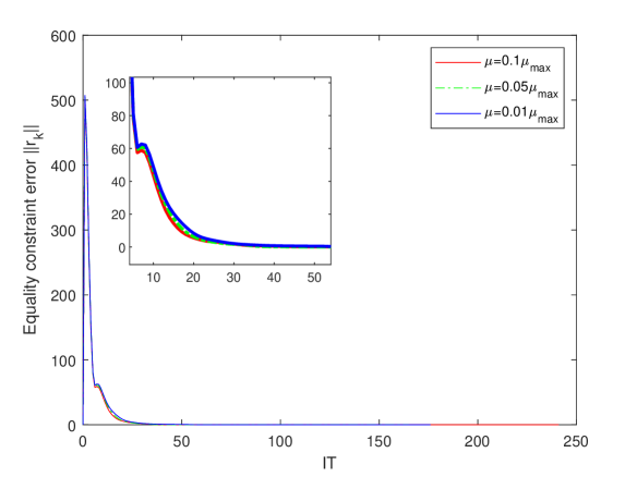
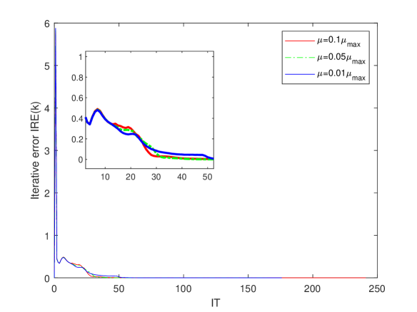
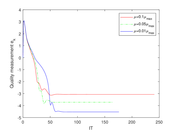
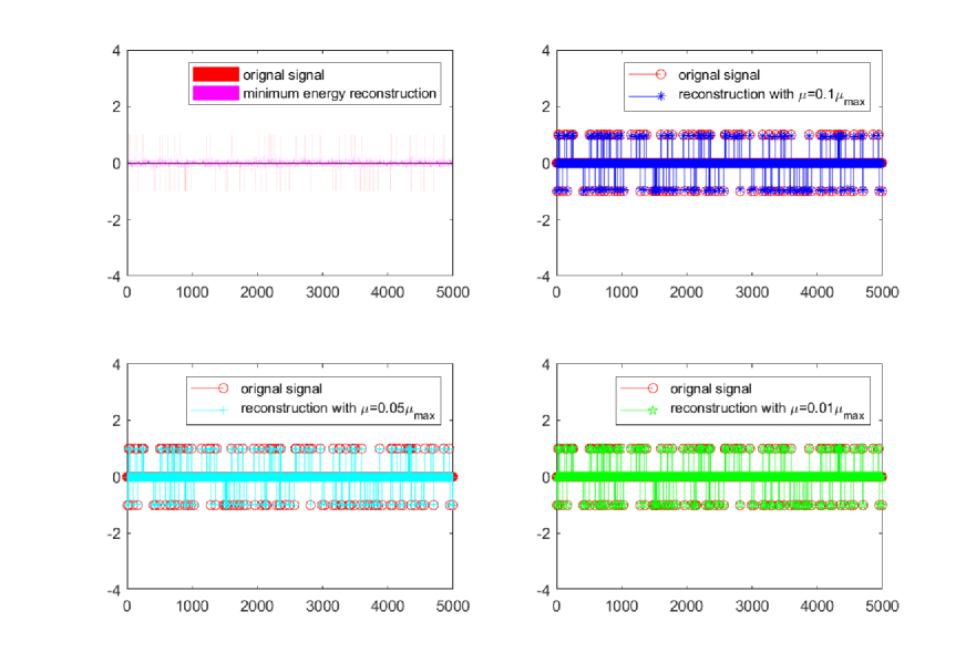
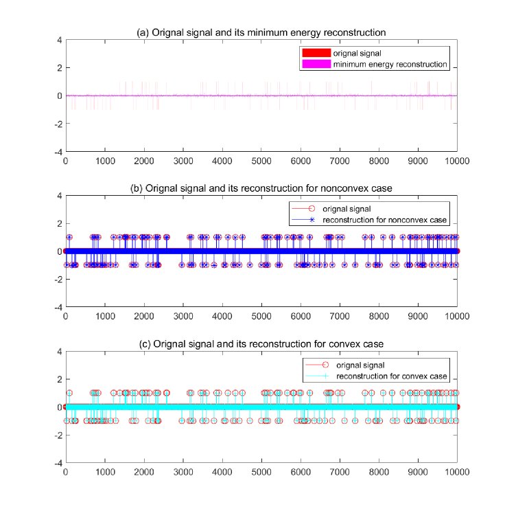
Next, we use the aforementioned codes to investigate the effect of regularization parameter $\mu$ on Algorithm 1.1 for solving the problem (3) with a large data $A\in\mathcal{R}^{2048\times 5000}$ and the same spikes, but the tolerance is set as $\epsilon=10^{-12}$. Fig. 1 depicts convergence behaviors of the equality constraint error $\|r_{k}\|$, the iterative error IRE(k) and the recovery signal quality $e_{k}:=\log_{10}\frac{\|\mathbf{x}_{k}-\mathbf{x}_{\textrm{orig}}\|}{\|\mathbf{x}_{\textrm{orig}}\|}$ along the iteration process after applying Algorithm 1.1 with $\mu=0.1\mu_{\max},\ 0.05\mu_{\max},\ 0.01\mu_{\max}$, respectively. Fig. 2 also presents the results to visualize the recovery quality of the signal versus the original signal, where the upper-left plot shows the minimum energy reconstruction signal $A^{\dagger}c$ (which is the point satisfying $A^{\sf T}A\mathbf{x}=A^{\sf T}c$) versus the original signal. An outstanding observation from Fig. 1 is that the smaller the value of $\mu$ is, the smaller the iteration number is (and the better the recovery quality of the signal is). After identifying the nonzero positions in the reconstructed signal, it always has the correct number of spikes for the case with $\mu=0.01\mu_{\max}$ and is closer to the original noiseless signal.

Fig. 2: Comparison between the original signal and reconstructed signal by Algorithm 1.1 for solving problem (3) with $(l,m)=(2048,5000)$ but with different regularization factor $\mu$.

		$l_{1/2}$	regularizer			$l_{1}$	regularizer
$(l,m)$	IT	CPU	EQU	$l_{2}$ error	IT	CPU	EQU	$l_{2}$ error
(1024, 3000)	358	16.37	4.60e-14	1.20e-2	501	22.60	1.93e-14	3.70e-2
(1024, 4000)	367	25.93	4.18e-14	1.28e-2	507	35.611	4.78e-14	4.26e-2
(2048, 5000)	215	30.65	2.84e-14	1.08e-2	250	36.01	3.27e-14	2.66e-2
(2048, 6000)	222	41.37	3.98e-14	1.20e-2	266	49.59	3.47e-14	3.07e-2
(3000, 7000)	201	58.08	2.71e-14	1.17e-2	231	66.91	2.93e-14	2.60e-2
(3000, 8000)	205	71.36	3.77e-14	1.10e-2	230	79.55	3.62e-14	2.58e-2
(4000, 9000)	199	97.52	3.29e-14	1.11e-2	231	112.94	2.87e-14	2.69e-2
(4000, 10000)	202	118.62	2.37e-14	1.03e-2	231	135.72	2.91e-14	2.51e-2

Table 2: Results of Algorithm 1.1 for (3) with different regularization terms and dimensions.

In the following, we use the proposed algorithm to solve two different cases of the sparse signal recovery problem to investigate which regularization term performs better: Case (i) the convex problem (2) with $l_{1}$ regularization term; Case (ii) the nonconvex problem (3) with $l_{1/2}$ regularization term. Table 2 reports some numerical results, where the problem dimension comes from 3000 to 10000 w.r.t the dimension of the signal, the regularization parameter is fixed as $\mu=0.01\mu_{\max}$ and Algorithm 1.1 is terminated under tolerance $\epsilon=10^{-15}$ with maximal iteration numbers 1000. Fig. 3 depicts comparison results between the original signal and the reconstructed signal for the signal dimension $m=10000$. First of all, it can be seen from results in Table 2 that the proposed algorithm is feasible for solving both the nonconvex and convex sparse signal recovery problem, especially for the large-scale problem. Besides, an obvious observation from Table 2 is that using $l_{1/2}$ regularizer is significantly better than $l_{1}$ regularizer to recover a signal, which could be checked from reported results of the iteration number, the CPU time and the recovery quality (i.e., $l_{2}$ error).

Fig. 3: Original signal and reconstructed signal by Algorithm 1.1 for solving the sparse signal recovery problem with $(l,m)=(4000,10000)$ but with different regularization terms.

Finally, we would apply the proposed algorithm to solve the direction-of-arrival (DOA) estimation problem [30] with a single snapshot. Here we consider a uniformly linear array of $M=100$ sensors with half-wavelength elements spacing. Let $\boldsymbol{\theta}=[\theta_{1},\cdots,\theta_{L}]^{\sf T}$ denote the $L$ angles of interest in $[-\frac{\pi}{2},\frac{\pi}{2}]$. Denote $\mathbf{x}=[x_{1},\cdots,x_{L}]^{\sf T}$ as the amplitudes of the potential signals from the $L$ incoming angles. Thus, the received signal at the sensor array is given by: $\mathbf{y}=A\mathbf{x}+\boldsymbol{n}$, where $\mathbf{y}=[y_{1},\cdots,y_{M}]^{\sf T}$, $\boldsymbol{n}=[n_{1},\cdots,n_{M}]^{\sf T}$, the steering matrix $A=[\mathbf{a}(\theta_{1}),\cdots,\mathbf{a}(\theta_{L})]$ and $\mathbf{a}(\theta_{l})=[1,\exp(-j\pi\sin(\theta_{l})),\cdots,\exp(-j\pi(M-1)\sin(\theta_{l}))]^{\sf T}$.

Fig. 4: The left and right are the errors and average run time versus different SNRs, respectively.

Fig. 5: DOAs at SNR$=5$dB.

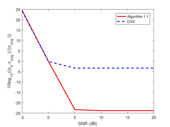
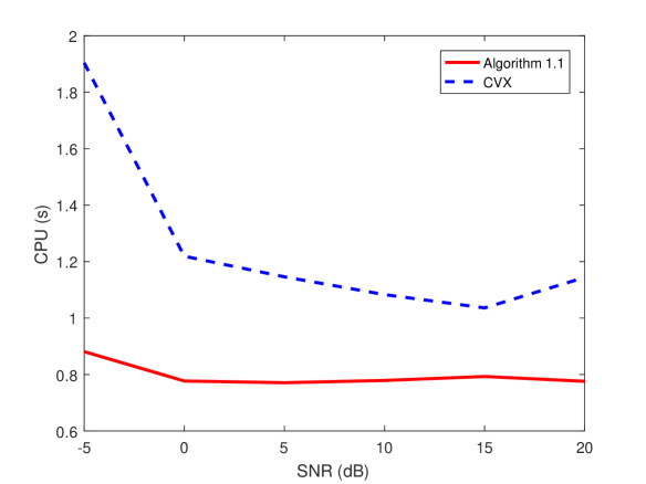
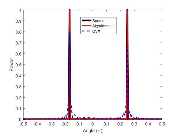
We consider the narrowband scenario with $K=2$ uncorrelated far-field source signals with normalized DOA parameters $-\frac{\pi}{6}$ and $\frac{\pi}{4}$. To run the proposed method, we divide the potential angle region $[-\frac{\pi}{2},\frac{\pi}{2}]$ into $L=180$ uniformly discrete grid points, i.e., $\boldsymbol{\theta}=\frac{\pi}{180}[-90,-89,\cdots,89,90]^{\sf T}$. When the signal-to-noise-ratio (SNR) varies from $-5$dB to $20$dB, i.e., $\{-5,0,5,10,15,20\}$dB, we implement the proposed method and the well-known CVX toolbox for $100$ Monte Carlo runs, and compute their root mean square errors and running time, as plotted in Fig. 4. For visible comparison, we plot the result from one Monte Carlo in the case of $5$dB, as shown in Fig. 5. From Figs. 4-5, we can see that:

• The accuracy of the two methods increases with the increase of SNR;

• The implementation of the proposed method is faster than that of the CVX method.

• In terms of DOA resolution and the estimation accuracy of the incoming signal power, the proposed method is better than that of CVX.

5 Conclusion remarks

In this paper, we construct a symmetric alternating direction method of multipliers for solving a family of possibly nonconvex nonxmooth optimization problems. Two different acceleration techniques are designed for fast convergence. Under proper assumptions, convergence of the proposed algorithm as well as its pointwise iteration complexity are analyzed in detail. By testing the so-called sparse signal recovery problem in signal processing with nonconvex/convex regularization terms and by using adaptively updating strategy for the penalty parameter, a number of numerical results demonstrate the feasibility and efficiency of the new algorithm and further show that the $l_{1/2}$ regularization term is better than the $l_{1}$ regularization term in terms of CPU time, iteration number and recovery error. Our future work will focus on solving stochastic nonconvex optimization problems by using a similar first-order algorithm to ADMM.

References

- [1]
- [2] H. Attouch, J. Bolte, P. Redont, A. Soubeyran, Proximal alternating minimization and projection methods for nonconvex problems: An approach based on the Kurdyka-Lojasiewicz inequality, Mathematics of Operations Research, 35 (2010) 438-457.
- [3] S. Boyd, N. Parikh, E. Chu, B. Peleato, J. Eckstein, Distributed optimization and statistical learning via the alternating direction method of multipliers, Foundations and Trends in Machine Learning, 3 (2010) 1-122.
- [4] J. Bai, H. Zhang, J. Li, A parameterized proximal point algorithm for separable convex optimization, Optimization Letters, 12 (2018) 1589-1608.
- [5] J. Bai, J. Li, F. Xu, H. Zhang, Generalized symmetric ADMM for separable convex optimization, Computational Optimization and Applications, 70 (2018) 129-170.
- [6] J. Bai, J. Li, Z. Wu, Several variants of the primal-dual hybrid gradient algorithm with applications, Numerical Mathematics: Theory, Methods and Applications, 12 (2019) 1-24.
- [7] R. Chartrand, V. Staneva, Restricted isometry properties and nonconvex compressive sensing, Inverse Problems, 24 (2008) 20-35.
- [8] X. Chang, S. Liu, P. Zhao, D. Song, A generalization of linearized alternating direction method of multipliers for solving two-block separable convex programming, Journal of Computational and Applied Mathematics, 357 (2019) 251-272.
- [9] E. Corman, X. Yuan, A generalized proximal point algorithm and its convergence rate, SIAM Journal on Optimization, 24 (2014) 1614-1638.
- [10] J. Douglas, H. Rachford, On the numerical solution of heat conduction problems in two and three space variables, Transactions of the American Mathematical Society, 82 (1956) 421-439.
- [11] J. Eckstein, D. Bertsekas, On the Douglas-Rachford splitting method and the proximal point algorithm for maximal monotone operators, Mathematical Programming, 55 (1992) 293-318.
- [12] M. Figueiredo, R. Nowak, S. Wright, Gradient projection for sparse reconstruction: application to compressed sensing and other inverse problems, IEEE Journal of Selected Topics in Signal Processing, 1 (2007) 586-597.
- [13] F. Fang, B. He, H. Liu, X. Yuan, Generalized alternating direction method of multipliers: new theoretical insights and applications, Mathematical Programming Computation, 7 (2015) 149-187.
- [14] D. Gabay, Applications of the method of multipliers to variational inequalities, Studies in Mathematics and Its Applications, 15 (1983) 299-331.
- [15] R. Glowinski, Lectures on numerical methods for non-linear variational problems, Published for the Tata Institute of Fundamental Research, Bombay [by] Springer-Verlag, 1980.
- [16] R. Glowinski, On alternating direction methods of multipliers: A historical perspective, In Modeling, Simulation and Optimization for Science and Technology, W. Fitzgibbon, Y.A. Kuznetsov, P. Neittaanmaki, O. Pironneau, eds., Computational Methods in Applied Sciences, Vol. 34, Springer, Dordrecht, (2014), 59-82.
- [17] R. Glowinski, T. Karkkainen, K. Majava, On the convergence of operator-splitting methods, in Numerical Methods for Scientific Computing, Variational Problems and Applications, E. Heikkola, Y. Kuznetsov, P. Neittaanmaki, and O. Pironneau, eds., CIMNE, Barcelona, 2003, pp. 67-79.
- [18] K. Guo, D. Han, T. Wu, Convergence of alternating direction method for minimizing sum of two nonconvex functions with linear constraints, International Journal of Computer Mathematics, 94 (2017) 1653-1669.
- [19] K. Guo, D. Han, D. Wang, T. Wu, Convergence of ADMM for multi-block nonconvex separable optimization models, Frontier of Mathematics in China, 12 (2017) 1139-1162.
- [20] K. Guo, D . Han, T. Wu, Convergence of ADMM for optimization problems with nonseparable nonconvex objective and linear constraints, Pacific Journal of Optimization, 14 (2018) 489-506.
- [21] M. Goncalves, J. Melo, R. Monteiro, Convergence rate bounds for a proximal ADMM with over-relaxation stepsize parameter for solving nonconvex linearly constrained problems, arXiv:1702.01850v2 (2017).
- [22] B. He, H. Liu, Z. Wang, X. Yuan, A strictly contractive Peaceman-Rachford splitting method for convex programming, SIAM Journal on Optimization, 24 (2014) 1011-1040.
- [23] B. He, H. Yang, S. Wang, Alternating direction method with self-adaptive penalty parameters for monotone variational inequalities, Journal of Optimization Theory and Applications, 106 (2000) 337-356.
- [24] B. He, F. Ma, X. Yuan, Convergence study on the symmetric version of ADMM with larger step sizes, SIAM Journal on Imaging Science, 9 (2016) 1467-1501.
- [25] M. Hong, Z. Luo, M. Razaviyay, Convergence analysis of alternating direction method of multipliers for a family of nonconvex problems, SIAM Journal on Optimization, 26 (2016) 337-364.
- [26] S. Kim, K. Koh, M. Lustig, S. Boyd, D. Gorinvesky, An interior-point method for large-scale -regularized least squares, IEEE Journal of Selected Topics in Signal Processing, 1 (2007) 606-617.
- [27] P. Lions, B. Mercier, Splitting algorithms for the sum of two nonlinear operators, SIAM Journal on Numerical Analysis, 16 (1979) 964-979.
- [28] G. Li, T. Pong, Global convergence of splitting methods for nonconvex composite optimization, SIAM Journal on Optimization, 25 (2015) 2434-2460.
- [29] Q. Liu, X. Shen, Y. Gu, Linearized ADMM for nonconvex non-smooth optimization with convergence analysis, IEEE Access, (2019) doi:10.1109/ACCESS.2019.2914461.
- [30] D. Malioutov, M. Cetin, A. Willsky, A sparse signal reconstruction perspective for source localization with sensor arrays, IEEE Transactions on Signal Processing, 53 (2005) 3010-3022.
- [31] B. Mordukhovich, Variational Analysis and Generalized Differentiation I: Basic Theory, Grundlehren der mathematischen Wissenschaften, Springer-Verlag Berlin Heidelberg, 2006.
- [32] Y. Nesterov, A method of solving a convex programming problem with convergence rate , Soviet Mathematics Doklady, 27 (1983) 372-376.
- [33] D. Peaceman, H. Rachford, The numerical solution of parabolic elliptic differential equations, SIAM Journal on Applied Mathematics, 3 (1955) 28-41.
- [34] R. Rockafellar, R. Wets, Variational Analysis, Springer-Verlag Berlin Heidelberg, 1998.
- [35] T. Sun, C. Zhang, Sparse matrix inversion with scaled Lasso, Journal of Machine Learning Research, 14 (2013) 3385-3418.
- [36] W. Wang, Y. Yin, J. Zeng, Global convergence of ADMM in nonconvex nonsmooth optimization, Journal of Scientific Computing, 78 (2019) 29-63
- [37] Z. Wu, M. Li, D. Wang, D. Han, A symmetric alternating direction method of multipliers for separable nonconvex minimization problems, Asia-Pacific Journal of Operational Research, 34 (2017) 1750030, 27 pages.
- [38] Z. Xu, X. Chang, F. Xu, H. Zhang, regularization: a thresholding representation theory and a fast solver, IEEE Transactions on Neural Networks and Learning Systems, 23 (2012) 1013-1027.
- [39] L. Yang, T. K. Pong, X. Chen, Alternating direction method of multipliers for a class of nonconvex and nonsmooth problems with applications to background/foreground extraction, SIAM Journal on Imaging Sciences, 10 (2017) 74-110.
- [40] M. Zhu, T. Chan, An efficient primal-dual hybrid gradient algorithm for total variation image restoration, CAM Report 08-34, UCLA, Los Angeles, CA, 2008.