Estimating adult death rates from sibling histories:
a network approach

Abstract

Hundreds of millions of people live in countries that do not have complete death registration systems, meaning that most deaths are not recorded and critical quantities like life expectancy cannot be directly measured. The sibling survival method is a leading approach to estimating adult mortality in the absence of death registration. The idea is to ask a survey respondent to enumerate her siblings and to report about their survival status. In many countries and time periods, sibling survival data are the only nationally-representative source of information about adult mortality. Although a huge amount of sibling survival data has been collected, important methodological questions about the method remain unresolved. To help make progress on this issue, we propose re-framing the sibling survival method as a network sampling problem. This approach enables us to formally derive statistical estimators for sibling survival data. Our derivation clarifies the precise conditions that sibling history estimates rely upon; it leads to internal consistency checks that can help assess data and reporting quality; and it reveals important quantities that could potentially be measured to relax assumptions in the future. We introduce the R package siblingsurvival, which implements the methods we describe.

1 Introduction

Death rates at adult ages are a core component of population health and a central topic of study for demography. Unfortunately, most of the world’s poorest countries are victims of the scandal of invisibility: they do not have complete death registration systems, meaning that most people die without ever having their existence officially recorded (Setel et al. 2007; AbouZahr et al. 2015). This lack of complete death registration means that critical quantities like life expectancy cannot be directly measured. Improving death registration systems is the long-term solution to the scandal of invisibility, but progress has been very slow (Mikkelsen et al. 2015). Until complete death registration systems are available everywhere, sample-based approaches to adult mortality estimation will continue to play a critical role in understanding population health and wellbeing.

The leading approach to collecting information about adult mortality in the absence of death registration is the sibling survival method (Rutenberg and Sullivan 1991; Brass 1975). The idea is to ask survey respondents to report the number of siblings they have, and to then ask for each sibling’s gender, date of birth and date of death (where appropriate). This data collection strategy produces sibling histories which contain information about the survival status of all of the members of the respondent’s sibship.

Since high-quality household surveys are routinely conducted in most countries—including countries that lack death registration systems—the sibling survival method offers the opportunity to try to estimate adult death rates in many places that have no other nationally-representative adult mortality data. Over the past two decades, a huge amount of sibling history data has been collected; for example, as a part of the DHS program alone, sibling histories have been collected in more than 150 surveys from dozens of countries around the world (Corsi et al. 2012; Fabic, Choi, and Bird 2012).

However, understanding how to analyze sibling histories has proven to be very challenging. Researchers have long been aware that the method suffers from many possible sources of bias (Gakidou and King 2006; Graham, Brass, and Snow 1989; Masquelier 2013; Reniers, Masquelier, and Gerland 2011; Trussell and Rodriguez 1990). Previous studies have concluded that sibling history estimates can be problematic if (i) there are sibships with no surviving members who could potentially be sampled and interviewed in the survey; (ii) more generally, there is a relationship between sibship size and mortality (e.g. larger sibships face higher death rates); and (iii) respondents’ reports about their siblings are inaccurate (e.g. respondents omit siblings or misreport a sibling’s survival status). There has also been confusion about whether the survival status of the respondent herself should be included in the calculations, since respondents are always alive (Masquelier 2013; Reniers, Masquelier, and Gerland 2011).

Researchers have worked on addressing these concerns about the sibling survival method in three main ways: they have collected empirical information about possible sources of bias in sibling reports (e.g., Helleringer, Pison, Kanté, et al. 2014); they have used microsimulation to illustrate how large certain sources of bias can be under different scenarios (Masquelier 2013); and they have used regression models to pool information from different countries and time periods (Gakidou and King 2006; Timaeus and Jasseh 2004; Obermeyer et al. 2010). Together, these studies have produced many important insights about the sibling survival method. However, these insights have not yet brought about a consensus on how sibling histories should be analyzed. Currently, there is partial evidence about many individual sources of possible bias, but there is no way to integrate all of this evidence together. Thus, even if we knew the exact size and direction of all the different sources of possible error, we still would not understand how the errors would combine to affect estimated death rates. More generally, little has been proven about the precise conditions under which sibling survival estimates can be expected to have attractive statistical properties such as consistency or unbiasedness.

In this study, our goal is to help resolve some of the methodological uncertainty about sibling survival. Our analysis is based on the insight that the sibling relation induces a particular type of social network among the members of a population. In this network, two people are connected to one another if they are siblings; thus, estimating death rates from sibling histories can be understood as a problem in network sampling. Starting from the principles of network reporting, we describe how to mathematically derive a sibling survival estimator. Deriving an estimator from first principles in this way enables us to (i) clarify the precise assumptions that the estimator requires in order to be consistent, unbiased, and efficient; (ii) describe how violations of any and all assumptions can combine to affect estimated death rates; (iii) identify quantities that could potentially be measured in the future to relax assumptions; and (iv) develop internal consistency checks that can be used to assess data and reporting quality in a given sample.

2 Setup

Figure 1 illustrates how we understand sibling histories as a network reporting problem. The left-hand panel shows a small population whose members are connected if they are siblings (i.e., two nodes are connected if they have the same mother). Clear nodes are alive and grey nodes are dead at the time of the survey. Since the sibling relation is transitive, the network is entirely composed of fully connected components, or cliques; each of these cliques is one sibship. The middle panel shows one specific sibship, and the right-hand panel illustrates the bipartite reporting network that is generated when all of the surviving members of that sibship are asked to report about their siblings. In the bipartite reporting network, each directed edge represents one sibling reporting about another—so, for example, the edge $13\rightarrow 12$ indicates that node 13 reports about node 12. Feehan and Salganik (2016a) describes bipartite reporting networks in greater detail.

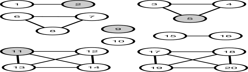
(a)

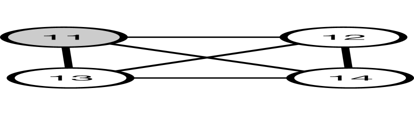
(b)

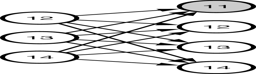
(c)

Figure 1: Framing sibling survival as a network reporting estimator. (a) A population connected through a sibship network. Because the sibling relation is transitive, the network is composed entirely of cliques. (b) The network for a single sibship. (c) Bipartite reporting graph for a single sibship.

Our quantity of interest is $M_{\alpha}$, the death rate for a specific group $\alpha$ (for example, $\alpha$ might be all women aged 30-34 in 2018). $M_{\alpha}$ is defined as

$$M_{\alpha}=\frac{D_{\alpha}}{N_{\alpha}},$$ (1)

where $D_{\alpha}$ is the number of deaths in group $\alpha$ and $N_{\alpha}$ is the person-years of exposure among members of group $\alpha$. We can develop an estimator for $M_{\alpha}$ by separately estimating the numerator and the denominator of Equation 1; thus, the challenge is to derive sibling history-based estimators for $D_{\alpha}$ and $N_{\alpha}$.

Figure 1c illustrates the fact that each sibling can potentially be reported as many times as she has living sibship members who are eligible to respond to the survey (Sirken 1970; Gakidou and King 2006; Masquelier 2013). Inferences from sibling reports must somehow account for this fact. Our approach is to distinguish between two groups of people: the first group is people who have no siblings who are eligible to respond to the survey. These people will never appear in the sibling history data – they are invisible to the sibling histories. The second group is visible people who do have siblings eligible to respond to the survey.

Formally, let $U$ be the population being studied, and let $F\subset U$ be the frame population, which is the set of all people who are eligible to respond to the survey. We define person $j\in U$’s visibility, $v(j,F)$, to be the number of living siblings who would report person $j$ in a census of $F$. Everyone in the population is either visible ($v(j,F)>0$) or invisible ($v(j,F)=0$). Thus, we can write the number of deaths in group $\alpha$ as:

$$D_{\alpha} =\underbrace{\sum_{\begin{subarray}{c}j\in D_{\alpha}\\ v(j,F)>0\end{subarray}}1}_{\text{ visible deaths }}+\underbrace{\sum_{\begin{subarray}{c}j\in D_{\alpha}\\ v(j,F)=0\end{subarray}}1}_{\text{ invisible deaths }}=D_{\alpha}^{V}+D_{\alpha}^{I},$$ (2)

where $D_{\alpha}^{V}$ is the number of visible deaths that could be learned about using sibling reports and $D_{\alpha}^{I}$ is the number of invisible deaths that cannot be learned about using sibling reports. We can define analogous quantities for the denominator $N_{\alpha}=N_{\alpha}^{V}+N_{\alpha}^{I}$, where the $N_{\alpha}^{V}$ is the visible exposure and $N_{\alpha}^{I}$ is the invisible exposure. Finally, we define $M_{\alpha}^{I}=\frac{D_{\alpha}^{I}}{N_{\alpha}^{I}}$ to be the invisible death rate, $M_{\alpha}^{V}=\frac{D_{\alpha}^{V}}{N_{\alpha}^{V}}$ to be the visible death rate, and $M_{\alpha}=\frac{D_{\alpha}^{I}+D_{\alpha}^{V}}{N_{\alpha}^{I}+N_{\alpha}^{V}}$ to be the total death rate.

In Section 3, we show how sibling history data can be used to develop death rate estimators for the visible population. We address possible differences between the visible and the invisible populations as part of a more general sensitivity framework, introduced in Section 4. Our sensitivity framework consists of mathematical expressions that describe how sensitive death rate estimates are to all of the conditions that the estimators rely upon, including differences between the visible and invisible populations; reporting errors; and structural variation in sibship networks. Section 5 contains an empirical illustration of our technical results using the 2000 Malawi Demographic and Health Survey. As part of our empirical demonstration, we discuss variance estimation, and we introduce empirical checks that researchers can perform to assess some of the conditions that sibling estimators rely upon. Section 6 compares the estimators we introduce, and discusses the implication of our results for practice. Finally, Section 7 concludes and outlines directions for future work.

3 Adjusting for visibility in sibling reports

The visible death rate can be estimated from sibling histories using an expression of the form

$$\widehat{M}^{V}_{\alpha}=\frac{\widehat{D}^{V}_{\alpha}}{\widehat{N}^{V}_{\alpha}},$$ (3)

where $\widehat{D}^{V}_{\alpha}$ is an estimator for the number of visible deaths in group $\alpha$ and $\widehat{N}^{V}_{\alpha}$ is an estimator for the amount of visible exposure in group $\alpha$. In order to estimate these two quantities, we face the challenge that even people who are visible to the sibling histories may still differ in the extent to which they are visible; for example, visible people from larger sibships may tend to have different death rates than visible people from smaller sibships. We address this challenge by introducing statistical estimators that adjust for how visible reported siblings are.

We consider two different approaches to adjusting for differential visibility: aggregate visibility estimation and individual visibility estimation. These two approaches lead to two different estimators for the visible death rate. In both cases, we start by describing how to derive population-level relationships, and then we use these population relationships as the basis for sample-based estimators.

The aggregate visibility approach

The aggregate visibility approach is based on the idea that reports about siblings can first be aggregated, and then the aggregated reports can be adjusted to account for visibility (Bernard et al. 1989; Rutstein and Guillermo Rojas 2006; Feehan and Salganik 2016a). To illustrate this approach, we first focus on reports about visible deaths among siblings, $D^{V}_{\alpha}$. Throughout the main paper, we assume there are no false positive reports – i.e., we assume that respondents’ reports may omit siblings, but that they never mistakenly include someone who is not truly a sibling. Of course, this could in fact happen – but this assumption makes the exposition much cleaner, and the results derived in the Appendixes consider reporting with false positives.

Let $y(F,D^{V}_{\alpha})$ be the total number of deaths that would be reported among respondents’ siblings in a census of the frame population. Appendix .B.4 shows that if there are no false positive reports, then the total number of reports about sibling deaths, divided by the average visibility of visible deaths, will be equal to the number of visible deaths:

$$D^{V}_{\alpha}=\frac{y(F,D^{V}_{\alpha})}{\bar{v}(D^{V}_{\alpha},F)}.$$ (4)

The idea is that in a census, the average death will be reported $\bar{v}(D^{V}_{\alpha},F)$ times; thus, the total number of reports about deaths, $y(F,D^{V}_{\alpha})$, can be divided by $\bar{v}(D^{V}_{\alpha},F)$ to recover the total number of visible deaths. Appendix .B.4 shows that a similar analysis can be applied to the denominator of the visible death rate, yielding

$$N^{V}_{\alpha}=\frac{y(F,N^{V}_{\alpha})}{\bar{v}(N^{V}_{\alpha},F)}.$$

Thus, in a census,

$$M^{V}_{\alpha}=\frac{D^{V}_{\alpha}}{N^{V}_{\alpha}}=\frac{y(F,D^{V}_{\alpha})}{y(F,N^{V}_{\alpha})}\cdot\frac{\bar{v}(N_{\alpha}^{V},F)}{\bar{v}(D_{\alpha}^{V},F)}.$$ (5)

Under the assumption that the visibility of deaths is the same as the visibility of exposure, $\bar{v}(D^{V}_{\alpha},F)=\bar{v}(N^{V}_{\alpha},F)$, and Equation 5 simplifies to the aggregate visibility estimand

$$M^{V}_{\alpha,\text{agg}}=\frac{y(F,D^{V}_{\alpha})}{y(F,N^{V}_{\alpha})}.$$ (6)

Finally, the population-level relationship in Equation 6 motivates the sample-based estimator (Appendix .E):

$$\widehat{M}^{V}_{\alpha,\text{agg}} =\frac{\sum_{i\in s}w_{i}~{}y(i,D^{V}_{\alpha})}{\sum_{i\in s}w_{i}~{}y(i,N^{V}_{\alpha})}.$$ (7)

Since this approach is based on adding together reports about all of the siblings, and then adjusting for the visibility of these aggregate reports, we call $\widehat{M}^{V}_{\alpha,\text{agg}}$ an aggregate visibility estimator (Feehan 2015; Feehan, Mahy, and Salganik 2017; Bernard et al. 1989). Appendix .E (Result .E.1) formally derives the estimator; the derivation reveals that this approach can be expected to produce essentially unbiased estimates as long as reports about siblings are accurate, and as long as there is no relationship between sibship visibility and mortality (i.e., as long as $\bar{v}(D^{V}_{\alpha},F)=\bar{v}(N^{V}_{\alpha},F)$).

The individual visibility approach

The individual visibility approach is based on the idea that reports about siblings can first be adjusted for visibility and then the adjusted reports can be aggregated (Sirken 1970; Gakidou and King 2006; Lavallee 2007; Feehan 2015). To illustrate this approach, consider reports about a specific deceased sibling $j\in D_{\alpha}$ that are made in a census of the frame population. Let $y(F,j)$ be the number of times that people in the frame population $F$ report the deceased sibling $j$. This quantity $y(F,j)$ will be equal to the visibility of $j$ to $F$, $v(j,F)$, as long as there are no false positive reports. Thus, for every visible sibling $j$, we have

$$\frac{y(F,j)}{v(j,F)}=1.$$ (8)

Summing over all visible deaths, we obtain

$$D_{\alpha}^{V}=\sum_{j\in D_{\alpha}^{V}}1=\sum_{j\in D_{\alpha}^{V}}\frac{y(F,j)}{v(j,F)}=\sum_{i\in F}\sum_{j\in D_{\alpha}^{V}}\frac{y(i,j)}{v(j,F)},$$ (9)

where the last step follows because $y(F,j)=\sum_{i\in F}y(i,j)$. Equation 9 expresses the number of visible deaths in terms of each survey respondent’s reported connections to each death ($y(i,j)$) and the visibility of each death ($v(j,F)$). In Appendix .B.2, we show that when reporting is accurate, the visibility of any dead sibling $j\in D_{\alpha}^{V}$, can be written as $v(j,F)=y(i,F)+1$ for any survey respondent $i$ who is in the same sibship as $j$. Using this relationship, Equation 9 can be re-written as

$$D_{\alpha}^{V}=\sum_{i\in F}\sum_{j\in D_{\alpha}^{V}}\frac{y(i,j)}{v(j,F)}=\sum_{i\in F}\sum_{j\in D_{\alpha}^{V}}\frac{y(i,j)}{y(i,F)+1}=\sum_{i\in F}\frac{y(i,D_{\alpha})}{y(i,F)+1},$$ (10)

where $y(i,F)$ is $i$’s reported number of siblings on the sampling frame. Equation 10 relates the population-level number of visible deaths $D^{V}_{\alpha}$ to survey respondents’ reports about deaths in their sibships, $y(i,D_{\alpha})$, and survey respondents’ reports about the number of frame population members in their sibships, $y(i,F)$.

A parallel argument, found in Appendix .B.2, reveals that when reporting is accurate, $N^{V}_{\alpha}$ can be written as

$$N^{V}_{\alpha} =\sum_{i\in F}\left[\underbrace{\frac{y(i,N_{\alpha}\cap F)}{y(i,F)}}_{\text{siblings in $F$}}+\underbrace{\frac{y(i,N_{\alpha}-F)}{y(i,F)+1}}_{\text{siblings not in $F$}}\right],$$ (11)

where $y(i,N_{\alpha}\cap F)$ is $i$’s reported number of siblings on the sampling frame who contributed exposure; and $y(i,N_{\alpha}-F)$ is $i$’s reported number of siblings not on the sampling frame who contributed exposure. Combining Equation 10 and Equation 11, we have the population-level individual visibility estimand:

$$M^{V}_{\alpha,\text{ind}} =\frac{\sum_{i\in F}\left[\frac{y(i,D_{\alpha})}{y(i,F)+1}\right]}{\sum_{i\in F}\left[\frac{y(i,N_{\alpha}\cap F)}{y(i,F)}+\frac{y(i,N_{\alpha}-F)}{y(i,F)+1}\right]}.$$ (12)

Finally, the population-level relationship in Equation 12 motivates a sample-based estimator for $M^{V}_{\alpha}$ (Appendix .F):

$$\widehat{M}^{V}_{\alpha,\text{ind}} =\frac{\sum_{i\in s}w_{i}~{}\left[\frac{y(i,D_{\alpha})}{y(i,F)+1}\right]}{\sum_{i\in s}w_{i}~{}\left[\frac{y(i,N_{\alpha}\cap F)}{y(i,F)}+\frac{y(i,N_{\alpha}-F)}{y(i,F)+1}\right]},$$ (13)

where $i$ indexes survey respondents in the probability sample $s$ and $w_{i}$ is $i$’s sampling weight. Since this approach is based on adjusting for the visibility of each individual reported sibling, we call it individual visibility estimation. Appendix .F formally derives the estimator in Equation 13 (Result .F.1), including the precise conditions required for it to provide consistent and essentially unbiased estimates of the visible death rate.

Relationship to previous work

To the best of our knowledge, our study is the first to derive the aggregate visibility estimator from first principles. However, the estimator itself is not new: the aggregate visibility estimator is probably the most common approach to estimating death rates from sibling history data. For example, Equation 7 is the estimator used to produce age-specific adult death rate estimates in all Demographic and Health Survey reports (Rutstein and Guillermo Rojas 2006). The estimator appears to have been first proposed in Rutenberg and Sullivan (1991), and it has since been the subject of several methodological analyses, including Masquelier (2013), Gakidou and King (2006), Hill et al. (2006), Timaeus and Jasseh (2004), Stanton, Abderrahim, and Hill (2000), and Garenne et al. (1997). By focusing on the networked structure of sibling relations, our derivation reveals that the aggregate visibility estimator is related to other network estimation approaches, including the network scale-up method (Bernard et al. 1989); and the network survival estimator (Feehan, Mahy, and Salganik 2017).

The individual visibility estimator has its origins in multiplicity sampling (Sirken 1970; Lavallee 2007; Feehan 2015). In the context of sibling survival, an estimator similar to the one derived here was introduced by Gakidou and King (2006) and then further discussed by Obermeyer et al. (2010) and Masquelier (2013). The actual individual estimator in Equation 13 is somewhat different from the one proposed by Gakidou and King (2006), but both are motivated by the idea that observed information can be used to adjust for visibility at the level of individual reports.

4 Framework for sensitivity analysis

Both the individual and aggregate visibility estimators rely on several conditions to guarantee that they will produce consistent and essentially unbiased estimates of the death rate. These conditions make precise longstanding concerns researchers have had about sibling survival estimates. For example, researchers have often worried that inaccurate reports about siblings may lead to biased death rate estimates; our results reveal exactly how reports about siblings must be accurate in order to produce consistent and essentially unbiased estimates of death rates. They also reveal precise quantities which could potentially be measured to adjust sibling reports to account for reporting errors.

Appendices .E and .F contain detailed derivations of the sensitivity frameworks for both the individual and aggregate visibility estimators; here, we present and discuss the results of that analysis. The simulation study in Appendix .J empirically illustrates the sensitivity frameworks and confirms their correctness.

4.1 Sensitivity of the aggregate visibility estimator

The relationship between the population death rate in group $\alpha$ and the aggregate visibility estimand can be written as:

$$M_{\alpha}=\underbrace{M^{V}_{\alpha,\text{agg}}}_{\begin{subarray}{c}\text{aggregate}\\ \text{visibility}\\ \text{estimand}\end{subarray}}\times\underbrace{\frac{\bar{d}^{V}(N_{\alpha},F)}{\bar{d}^{V}(D_{\alpha},F)}}_{\begin{subarray}{c}\text{visibility}\\ \text{ratio}\end{subarray}}\times\underbrace{\frac{\gamma(F,N_{\alpha})}{\gamma(F,D_{\alpha})}}_{\begin{subarray}{c}\text{reporting}\\ \text{accuracy}\end{subarray}}\times\underbrace{\left[1+p^{I}_{N_{\alpha}}(K-1)\right].}_{\begin{subarray}{c}\text{difference between}\\ \text{invisible and}\\ \text{visible populations}\end{subarray}}$$ (14)

Equation 14 shows that the visible death rate can be decomposed into the product of the aggregate visibility estimand and several adjustment factors. When all of these adjustment factors are equal to 1, the aggregate visibility estimand is equal to the total death rate.

The first group of adjustment factors–called the visibility ratio– describes how a relationship between visibility and mortality would affect estimated death rates. It is the ratio of the average visibility of all siblings who contribute to exposure ($\bar{d}^{V}(N_{\alpha},F)$) and the average visibility of siblings who die ($\bar{d}^{V}(D_{\alpha},F)$). When there is no relationship between these two quantities, the visibility ratio will be 1. When, say, siblings who have died tend to be in less visible sibships than siblings overall, then this factor will tend to be greater than 1 (meaning that the death rate will be under-estimated).

The next group of adjustment factors captures the extent to which reports about siblings are accurate. It is the ratio of a quantity that captures the net accuracy of reports about exposure ($\gamma(F,N_{\alpha})$) and a quantity that captures the net accuracy of reports about deaths ($\gamma(F,D_{\alpha})$). Two particularly salient findings emerge from the derivation of this group of adjustment factors (Appendix .E): first, the estimator requires that reporting be accurate in aggregate, but not necessarily at the individual level; as long as reporting errors across individuals cancel one another out, estimates will not be affected. Second, this group of adjustment factors shows that aggregate visibility estimates will not be affected if reporting errors about deaths and reporting errors about exposure balance out. In other words, if respondents tend to, say, omit older siblings at a constant rate, independent of the survival status of older siblings ($\gamma(F,D_{\alpha})=\gamma(F,N_{\alpha})<1$), then Equation 14 reveals that death rates can still be accurate because reporting errors about deaths and about exposure will cancel out. Thus, Equation 14 reveals that the death rate estimator can be robust to situations in which respondents’ reports are imperfect, but imperfect in similar ways for siblings who die and siblings who survive.

Finally, the last group captures the conditions needed to be able to use only information about visible deaths to estimate the total death rate. This group depends on two quantities: $p^{I}_{N_{\alpha}}$, the amount of exposure that is invisible; and $K=\frac{M^{I}_{\alpha}}{M^{V}_{\alpha}}$, an index for how different the invisible and visible death rates are. Below, in Section 5, we will use an empirical example to illustrate this group of adjustment factors in more depth.

4.2 Sensitivity of the individual visibility estimator

The derivation in Appendix .F reveals that the relationship between the population death rate in group $\alpha$ and the individual visibility estimand can be written as:

$$M_{\alpha} =\underbrace{M^{V}_{\alpha,\text{ind}}}_{\begin{subarray}{c}\text{individual}\\ \text{visibility}\\ \text{estimand}\end{subarray}}\times\underbrace{\frac{\bar{\gamma}^{\star}_{N}~{}(1+K_{N})}{\bar{\gamma}_{D}~{}(1+K_{D})}}_{\begin{subarray}{c}\text{reporting}\\ \text{accuracy}\end{subarray}}\times\underbrace{\left[1+p^{I}_{N_{\alpha}}(K-1)\right].}_{\begin{subarray}{c}\text{difference}\\ \text{between}\\ \text{visibile and}\\ \text{invisibile populations}\end{subarray}}$$ (15)

Equation 15 again decomposes the population death rate into the product of the individual visibility estimand and several groups of adjustment factors. The main insights from Equation 14 also apply to the individual visibility expression in Equation 15. However, it is worth noting a few differences between the two frameworks. First, note that Equation 15 does not have any adjustment factors related to a visibility ratio. This is an advantage of the individual visibility estimator: it does not need to make any assumptions about the absence of a relationship between visibility and mortality (within the visible population). Second, the individual visibility expression in Equation 15 has a more complex set of adjustment factors that capture reporting accuracy. This more complex expression describes the extent to which reporting errors are correlated with reports about deaths and reports about exposure; for example, if reporting tends to omit deaths in sibships that have more deaths, then $K_{D}>1$. More generally, even if deaths and exposure are under-reported at the same average rate, so that the average reporting adjustment factor is equal to 1, there can still be problems if the reporting errors are different in how they are correlated with the number of sibship deaths and exposure. In general, reporting errors appear to be more complex under the individual visibility estimator; we will discuss the implications of this in Section 6.

5 Empirical illustration

We motivate our technical results with an empirical example: the sibling history data from the 2000 Malawi Demographic and Health Survey (Malawi National Statistical Office and ORC Macro 2001). We chose this example for two reasons: first, we wanted the empirical example to be a Demographic and Health Survey, since DHS surveys are the largest available source of sibling history data; as we write, more than 150 DHS surveys in 60 countries have collected sibling histories over a period of about 30 years. Second, among Demographic and Health Surveys, we chose the 2000 Malawi DHS because it had low missingness in sibling reports, and because its sample size of 13,220 women was close to average. Our analysis of the 2000 Malawi DHS sibling histories uses the siblingsurvival R package, which we created as a companion to this paper.

Figure 2 shows estimated death rates and confidence intervals for male and female death rates in Malawi over the seven year period before interviews were conducted. For males, the individual and aggregate visibility estimates are qualitatively quite similar. For females, however, aggregate visibility estimates are systematically higher than individual visibility estimates, and these differences are larger than the estimated sampling variation. We discuss a possible explanation for this difference in more detail in Appendix .G.3.

5.1 Variance estimation

Researchers need to be able to estimate the sampling uncertainty of death rate estimates calculated using Equation 7 and Equation 13. We recommend that researchers use a resampling approach called the rescaled bootstrap to do so (Rao and Wu 1988; Rao, Wu, and Yue 1992). The rescaled bootstrap is appealing because (i) it accounts for the complex sampling design that is typical of surveys like the DHS; (ii) it enables researchers to use a single approach to estimating the sampling uncertainty for death rates and for other quantities (such as the internal consistency checks we introduce below); and (iii) it has been successfully applied to other network reporting studies (e.g. Feehan, Mahy, and Salganik 2017). The siblingsurvival package uses the rescaled bootstrap to provide estimated sampling uncertainty for death rate estimates.

An alternate approach to estimating sampling uncertainty is to derive a mathematical expression that relates sampling variation to a function of study design parameters and population characteristics that are known or that can be approximated; this approach is discussed in Appendix .I, where we illustrate how linearization can be used to derive an approximate variance estimator for estimated death rates. In practice, we expect the bootstrap approach discussed here to be most useful in empirical analyses.

Figure 2 shows confidence intervals for estimated male and female death rates in Malawi over the seven year period before interviews were conducted. To compare the amount of estimated sampling uncertainty for the aggregate and individual visibility estimates in Figure 2, we define the relative standard error of an estimate of $\widehat{M}^{V}_{\alpha}$ to be $\frac{\widehat{\text{se}}(\widehat{M}^{V}_{\alpha})}{\widehat{M}^{V}_{\alpha}}$, where $\widehat{\text{se}}(\widehat{M}^{V}_{\alpha})$ is the rescaled bootstrap estimated standard error. We then calculate the average of these relative standard errors across all age-sex groups for each estimator. The results suggest that the individual visibility estimator has slightly larger sampling variance than the aggregate visibility estimator (Table 1). This empirical finding is consistent with simulation results discussed in Appendix .J.

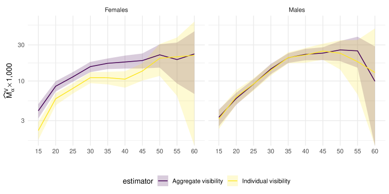
Figure 2: Aggregate and individual visibility estimates for log-adult death rates from the Malawi 2000 DHS sibling histories. Estimates are for the 7 years prior to the interview. Confidence bands show sampling uncertainty, accounting for the complex sample design; they were produced using the rescaled bootstrap method (Rao and Wu 1988; Feehan and Salganik 2016b).

Table 1: Comparison in average relative standard error for aggregate and individual visibility estimates of death rates across all ages for males and for females.

	Estimated Average Relative Standard Error
Estimator	Females	Males
Aggregate visibility	0.16	0.18
Individual visibility	0.21	0.25

5.2 Applying the sensitivity framework

Sensitivity to invisible deaths

Equation 14 expresses the difference between the visible and total death rate in terms of two parameters: $K$, an index for how different the visible and invisible death rates are; and $p^{I}_{N_{\alpha}}$, the proportion of exposure that is invisible. It is impossible to know the fraction of exposure that is invisible, $p^{I}_{N_{\alpha}}$, from sibling history data. However, we can try to approximate this quantity by taking advantage of the fact that we have a random sample of the frame population that is currently alive. We can use the sample to estimate what fraction of respondents would be invisible to sibling histories at the time of the survey, i.e., what fraction of survey respondents have no siblings on the sampling frame.

Figure 3a shows the estimated fraction of respondents to the 2000 Malawi DHS who would not be visible to sibling histories. As our derivations reveal, it is this visibility—and not sibship size per se—that matters for estimating death rates. Figure 3a gives an approximate sense for the type of values that we might expect to see for $p^{I}_{N_{\alpha}}$ by age. Figure 3a reveals that the share of respondents that is invisible has a U-shaped relationship with age, reaching its highest levels among the youngest and oldest survey respondents. This relationship is likely due to the definition of the frame population, which included women aged 15-49; age groups close to the boundaries of the frame population will tend to have siblings who are too old or too young to be included as respondents, reducing the visibility of these ages. At worst, about 40% of women at ages 45-49 would be invisible to sibling histories and at best, only about 15% of women ages 30-34 would be invisible to sibling histories.

What difference would this range of invisibility make to death rate estimates? The sensitivity relationship in Equation 14 reveals that the answer relies upon understanding how different death rates are in the invisible and visible populations. Figure 3b illustrates by showing the relative error that would result from a range of differences between invisible and visible death rates from 20% higher death rates in the invisible population to 20% lower death rates in the invisible population ($K$ parameter, shown on the y-axis) and a range of different proportions of exposure that is invisible, from 15% of exposure invisible to 30% of exposure invisible ($p^{I}_{N_{\alpha}}$, shown on the x axis). Even relatively large values for the two parameters appear to result in modest relative errors.

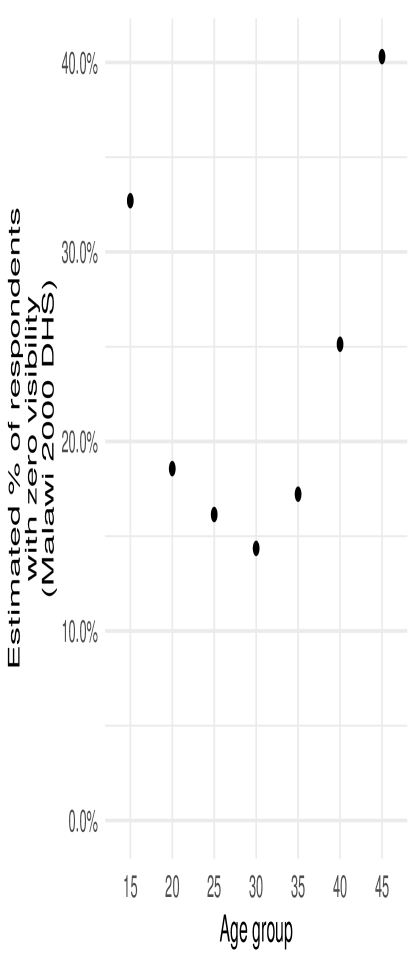
(a)

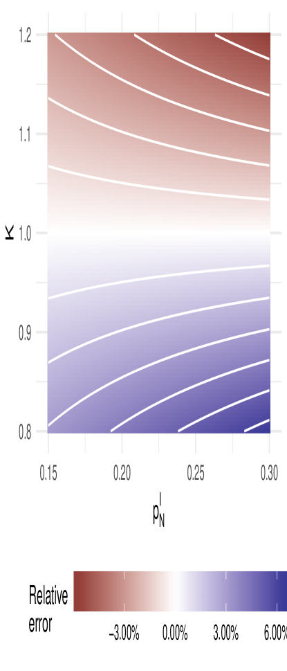
(b)

Figure 3: Sensitivity to invisible deaths.
(a) Estimated fraction of respondents to the Malawi 2000 DHS who would not be visible in sibling history data.
(b) Illustration of the relative error in using the visible death rate $M^{V}$ as an estimate for the total death rate $M$. The proportion of exposure that is invisible, $p^{I}_{N_{\alpha}}$, varies along the x axis; the relationship between the visible and invisible death rates, captured by the parameter $K$ (Equation 40), varies along the y axis. The colors show the percentage relative error; so if 20% of the population’s exposure is invisible ($p^{I}_{N_{\alpha}}=0.2$) and the invisible death rate is 10% higher than the visible death rate ($K=1.1$), the relative error is about 2 percent. Relative error increases as $K$ gets farther away from 1 and as $p^{I}_{N_{\alpha}}$ increases.

Reporting errors

Researchers have long been aware that reporting errors may affect the quality of sibling survival estimates. We will illustrate two ways to assess the sensitivity of aggregate visibility estimates to reporting errors. First, we will use Equation 14 to assess how much death rate estimates are affected by different levels of reporting error. Second, we will illustrate how our network reporting framework leads to data quality checks that can be performed on sibling history data.

5.2.1 Analyzing the impact of reporting errors using the sensitivity framework

We will illustrate the sensitivity framework by focusing on aggregate visibility estimates for brevity. The sensitivity framework in Equation 14 shows that reporting errors will affect the accuracy of aggregate visibility estimates through the ratio of two parameters: $\gamma(F,N_{\alpha})$ and $\gamma(F,D_{\alpha})$. Importantly, in principle it is possible to design a study that could measure $\gamma(F,N_{\alpha})$ and $\gamma(F,D_{\alpha})$. In fact, some promising research on the sibling method to date has compared sibling reports to ground truth information at a demographic surveillance site in southeastern Senegal (e.g., Helleringer, Pison, Kanté, et al. 2014). Studies like Helleringer, Pison, Kanté, et al. (2014) were designed to estimate somewhat different reporting parameters from $\gamma(F,D_{\alpha})$ and $\gamma(F,N_{\alpha})$; thus, there is not currently any direct evidence about these parameters available. However, to illustrate our sensitivity framework, we can base some back of the envelope calculations on the data reported by Helleringer and colleagues. Suppose that respondents never mistakenly count non-siblings as siblings but that, on average, about four percent of living siblings in group $\alpha$ get omitted by respondents’ reports, and about nine percent of dead siblings in group $\alpha$ get omitted by respondents’ reports. Then $\gamma(F,N_{\alpha})\approx 0.96$ and $\gamma(F,D_{\alpha})\approx 0.91$. If these approximations were correct, Equation 14 shows that, in order to adjust for reporting errors, the estimated death rates should be multiplied by about $\frac{0.95}{0.91}=1.05$. In other words, under this scenario, the unadjusted aggregate visibility estimator produces estimates that have a relative error of about 5% because of imperfect reporting.

5.2.2 Internal consistency checks

A second strategy for assessing sensitivity to reporting errors is to perform data quality checks on sibling history data (e.g., Helleringer, Pison, Masquelier, et al. 2014; Masquelier and Dutreuilh 2014; Stanton, Abderrahim, and Hill 2000; Garenne and Friedberg 1997; Rutenberg and Sullivan 1991). We now show how our reporting framework enables us introduce several new internal consistency checks that can be used to assess how accurate sibling reports are. The idea is to use the network reporting framework to identify several quantities that can be estimated in two different ways using independent subsets of the sibling history data (e.g., Feehan and Cobb 2019). If reporting is highly accurate, then we expect these independent estimates to agree; when these independent estimates are very different, that suggests that there may be considerable amounts of reporting error.

We base our internal consistency checks on reports about siblings’ ages. For a particular age, say 30, the symmetry of the sibling relation guarantees that in a census of the frame population,

$$\begin{subarray}{c}\text{\# connections people in $F$ aged 30}\\ \text{report to sibs in $F$ not aged 30}\end{subarray}=\begin{subarray}{c}\text{\# connections people in $F$ not aged 30}\\ \text{report to sibs in $F$ aged 30}\end{subarray}.$$ (16)

The quantity on the left-hand side of Equation 16 can be estimated from the survey respondents aged 30, and the quantity on the right-hand side of Equation 16 can be estimated from all of the survey respondents who are not aged 30. These two estimates can then be compared; if reporting is accurate, then we expect the estimates to agree.

Formally, for age $\alpha$, we write $y(F_{\alpha},F_{-\alpha})$ for the total reported connections from respondents aged $\alpha$ to siblings who are in $F$ but not aged $\alpha$; similarly, we write $y(F_{-\alpha},F_{\alpha})$ for the total reported connections from respondents not aged $\alpha$ to siblings who are in $F$ and who are age $\alpha$. In theory, these are same quantity. From sibling history data, we can independently estimate $y(F_{\alpha},F_{-\alpha})$ and $y(F_{-\alpha},F_{\alpha})$ and then compare how similar these two independent estimates of the same quantity are by calculating $\Delta_{\alpha}$:

$$\Delta_{\alpha}=\widehat{y}(F_{\alpha},F_{-\alpha})-\widehat{y}(F_{-\alpha},F_{\alpha}).$$

When the two estimates agree, $\Delta_{\alpha}$ is close to zero. If there is considerable reporting error, then $\Delta_{\alpha}$ can be very different from zero.

Figure 4 illustrates this idea by showing internal consistency checks for each age from the 2000 Malawi DHS sibling histories (Malawi National Statistical Office and ORC Macro 2001). The figure shows an internal consistency check based on each age from 15 to 49. Each point shows the difference between two independent estimates for the same quantity. If these independent estimates agreed perfectly, they would all lie on the horizontal $y=0$ line. The confidence intervals capture estimated sampling variation. Most of the confidence intervals include 0, suggesting that reports are internally consistent; however, the figure also suggests that there is some misreporting, particularly between ages 20 and 25.

In general, we expect that plots or quantitative summaries of internal consistency checks like Figure 4 will be a useful way for researchers to assess the face validity of sibling history data. As we describe below, these internal consistency relationships could also form the basis for developing model-based approaches to analyzing sibling histories.

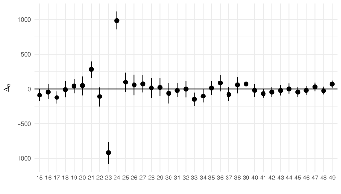
Figure 4: Internal consistency checks using sibling reports from the 2000 Malawi DHS sibling histories. Each point shows the difference between two independent estimates for the same quantity. If these independent estimates agreed perfectly, they would all lie on the horizontal $y=0$ line. Most of the checks’ confidence intervals include 0, suggesting that reports are internally consistent. However, the figure also suggests that there is some misreporting, particularly between ages 20 and 25. Confidence intervals show sampling uncertainty, accounting for the complex sample design; they were produced using the rescaled bootstrap method (Rao and Wu 1988; Feehan and Salganik 2016b).

6 Recommendations for practice

Should the respondent be included in the denominator?

The sibling survival literature has debated whether or not respondents should be included in the sibling reports. The concern is that respondents are, by definition, alive: thus, it seems possible that including respondents will bias estimated death rates downwards (Trussell and Rodriguez 1990; Masquelier 2013). The estimates published in DHS reports, which use the aggregate visibility estimator, do not include the respondent. More recently, Gakidou and King (2006) argued that respondents should be included in sibling reports, but this was disputed by Masquelier (2013).

In our framework, deciding to include or not include respondents in the denominator of the estimator amounts to deciding upon the definition of the visible and invisible populations. Since sibling history methods estimate a visible death rate, the question is: which visible population’s death rate is more likely to be a good estimate for the total population death rate $M_{\alpha}$?

To address this question, we analyzed the difference between the two visible populations in Appendix .G.1. Recall that $M^{V}_{\alpha}=\frac{D^{V}_{\alpha}}{N^{V}_{\alpha}}$ is the visible death rate when respondents are excluded from sibling histories, and let $M^{\prime V}_{\alpha}=\frac{D^{\prime V}_{\alpha}}{N^{\prime V}_{\alpha}}$ be the visible population when respondents are included in the reports. In Appendix .G.1, we show that the relationship between $M^{V}_{\alpha}$ and $M^{\prime V}_{\alpha}$ can be written as

$$M^{V}_{\alpha} =\frac{D^{V}_{\alpha}}{N^{V}_{\alpha}}=\frac{D^{\prime V}_{\alpha}}{N^{\prime V}_{\alpha}-C},$$ (17)

where $C$ is the number of people who contribute exposure and who have visibility of exactly 1 when respondents are included in the denominator; that is, $C$ is the number of people in the population who are in group $\alpha$, are eligible to respond to the survey, and who have no siblings who would be eligible to respond to the survey. $C$ will tend to be bigger, inducing a bigger difference between $M^{\prime V}_{\alpha}$ and $M^{V}_{\alpha}$, when (i) there is more overlap between the group $\alpha$ and the frame population; and, (ii) visibilities tend to be smaller, meaning that more people have a visibility exactly equal to 1 when respondents are included in the denominator.

Equation 17 reveals that the decision to include respondents in reports will move some people into the denominator, but it can never move anyone into the numerator.

A model developed in Appendix .G.2 shows that, in a simple situation in which everyone has the same probability of dying, it is most natural to exclude respondents from sibling reports. Under the model, when respondents are excluded, the invisible and visible populations have the same death rate, and that death rate can be estimated from sibling reports. Including respondents, on the other hand, induces a difference between the death rate in the visible and invisible population (even though every individual faces the same probability of death). Thus, our model suggests that excluding respondents from reports is preferable, at least in the simple world it describes. This conclusion agrees with the earlier modeling work of Trussell and Rodriguez (1990), which also argued that respondents should be excluded from reports.

However, these are suggestive results: without additional information, there is no way to be certain that $M^{V}_{\alpha}$ or $M^{\prime V}_{\alpha}$ will produce a better approximation to the population death rate $M_{\alpha}$ in a given population. The estimates presented here exclude respondents from reports, but we note that the full derivations of all of our estimators in Appendixes .F and .E cover both including and not including the respondent in the denominator. Thus, researchers who wish to include respondents in the denominator of the death rate can find the appropriate estimators there.

Aggregate vs individual visibility estimator

Our analysis suggests that there are strengths and limitations to both the individual and aggregate visibility estimators. Aggregate visibility estimates are typically based on the assumption that the visibility of deaths and the visibility of exposure are equal. The individual visibility estimator avoids this assumption altogether; thus, in situations where no information about adjustment factors is available, we recommend using the individual visibility estimator. In Appendix .G.3, we analyze the difference in aggregate and individual visibility estimates for Malawi, and we show that it is likely that this visibility assumption explains most of the difference between death rate estimates for females in Figure 2.

The individual visibility estimator has some disadvantages. Table 1 and the simulation study in Appendix .J suggest that the individual visibility estimator has slightly higher sampling variance than the aggregate visibility estimator. We hope that future research will continue to systematically compare the aggregate and individual visibility estimators; in the meantime, our view is that the individual visibility estimator’s relatively small loss in precision is a price that is worth paying to avoid having to make assumptions about the visibility of deaths and exposure.

Another disadvantage of the individual visibility estimator comes from the comparing the aggregate sensitivity framework (Equation 14) with the individual sensitivity framework (Equation 15). This comparison reveals that the quantities that would be needed adjust the individual visibility estimator for reporting error are much more complex than the analogous quantities needed to adjust the aggregate visibility estimator. Thus, if data that can be used to estimate adjustment factors become more widely available, then we expect the relative appeal of the aggregate visibility estimator to increase.

To recap, we recommend excluding respondents from reports. We also recommend using the individual visibility estimator in the absence of any empirical estimates for adjustment factors. However, we expect empirical information about adjustment factors to be much easier to collect for the aggregate visibility estimator. Thus, as empirical information about adjustment factors becomes available, we expect the aggregate visibility estimator to be more attractive. In all cases, we recommend that researchers who produce sibling history-based estimates use the sensitivity frameworks to assess how estimated death rates are affected by the assumptions used to produce them.

7 Discussion and Conclusion

We showed how sibling history data can be understood as a type of network reporting. We explained how to derive network-based estimators for adult death rates, how to devise internal consistency checks, and how to understand how sensitive death rate estimates can be to the different conditions that the estimators rely upon. We illustrated with an empirical example, based on our freely available R package siblingsurvival, and we outlined several recommendations for practitioners who wish to estimate death rates from sibling histories.

We see several important avenues for future research. Methodologically, a deeper comparison between the individual and aggregate visibility estimators would be useful. In particular, analytic results could help better understand our empirical finding that the individual visibility estimator has somewhat higher sampling variance than the aggregate visibility estimator. This analysis could also produce insights that might be useful for designing future data collection.

Our results also suggest next steps for developing models for death rate estimates based on sibling histories. This paper has focused on design-based estimators for death rates using sibling histories. Future research can use these design-based estimators as the starting point for developing model-based estimators. For example, the internal consistency checks that we discuss could form the basis for model-based adjustments of sibling reports (see McCormick, Salganik, and Zheng (2010) for a similar approach that has been developed in the context of aggregate relational data). Our framework also offers a natural way to think about how to pool information across countries and time periods.

We believe that collecting more information on sibling reports from settings where gold-standard adult death rates are available is crucial; Helleringer, Pison, Kanté, et al. (2014) is a useful template for the type of study design that could help produce more information. This type of study investigates the properties of sibling history reports in small areas where a gold-standard underlying truth about adult death rates is available. Data collected in this way can produce the information needed to estimate the adjustment factors in the individual and aggregate visibility sensitivity relationships. Combined with the framework we introduce here, estimates for these adjustment factors could provide a principled way to adjust national-level sibling survival estimates from surveys like the DHS, relaxing the conditions required for the estimates to be accurate.

Our analysis focused on death rate estimates for the time period immediately preceding the survey. In principle, the estimators discussed here could also be used for more distant time periods; however, the assumptions–though mathematically the same–presumably get stronger farther into the past. Future work could investigate this topic in more depth.

Our framework can also be applied to other demographic estimation techniques related to sibling survival, such as methods in which people report about their parents, spouses, or children (Hill et al. 1983; Moultrie et al. 2013). More generally, ideas from the sibling survival literature can be used to develop new methods for collecting data that have the potential to overcome some of the limitations of sibling histories. Feehan, Mahy, and Salganik (2017) explored how reports about two social network relationships could form the basis for death rate estimates at adult ages (see also Feehan et al. (2016)). Future research could continue to explore how to collect reports about more general types of relations, such as broader kin relationships or other types of social networks, with the goal of producing information that is timely and accurate enough to estimate adult death rates.

References

AbouZahr, Carla, Don de Savigny, Lene Mikkelsen, Philip W. Setel, Rafael Lozano, and Alan D. Lopez. 2015. “Towards Universal Civil Registration and Vital Statistics Systems: The Time Is Now.” The Lancet. http://www.sciencedirect.com/science/article/pii/S0140673615601702.

Bernard, H. Russell, Eugene C. Johnsen, Peter D. Killworth, and Scott Robinson. 1989. “Estimating the Size of an Average Personal Network and of an Event Subpopulation.” In The Small World, edited by Manferd Kochen, 159–75. Norwood, NJ: Ablex Publishing.

Brass, William. 1975. “Methods for Estimating Fertility and Mortality from Limited and Defective Data.” Methods for Estimating Fertility and Mortality from Limited and Defective Data. http://www.cabdirect.org/abstracts/19762901082.html.

Corsi, Daniel J., Melissa Neuman, Jocelyn E. Finlay, and S. V. Subramanian. 2012. “Demographic and Health Surveys: A Profile.” International Journal of Epidemiology 41 (6): 1602–13. http://ije.oxfordjournals.org/content/41/6/1602.short.

Fabic, Madeleine Short, YoonJoung Choi, and Sandra Bird. 2012. “A Systematic Review of Demographic and Health Surveys: Data Availability and Utilization for Research.” Bulletin of the World Health Organization 90 (8): 604–12. http://www.scielosp.org/scielo.php?pid=S0042-96862012000800012/&script=sci_arttext.

Feehan, Dennis M. 2015. “Network Reporting Methods.” PhD thesis, Princeton University. http://gradworks.umi.com/37/29/3729745.html.

Feehan, Dennis M., and Curtiss Cobb. 2019. “Using an Online Sample to Learn About an Offline Population.” arXiv:1902.08289 [Stat], February. http://arxiv.org/abs/1902.08289.

Feehan, Dennis M., Mary Mahy, and Matthew J. Salganik. 2017. “The Network Survival Method for Estimating Adult Mortality: Evidence from a Survey Experiment in Rwanda.” Demography 54 (4): 1503–28. https://link.springer.com/article/10.1007/s13524-017-0594-y.

Feehan, Dennis M., and Matthew J. Salganik. 2016a. “Generalizing the Network Scale-up Method: A New Estimator for the Size of Hidden Populations.” Sociological Methodology 46 (1): 153–86. http://128.84.21.199/pdf/1404.4009.pdf.

———. 2016b. Surveybootstrap: Tools for the Bootstrap with Survey Data. https://CRAN.R-project.org/package=surveybootstrap.

Feehan, Dennis M., Aline Umubyeyi, Mary Mahy, Wolfgang Hladik, and Matthew J. Salganik. 2016. “Quantity Versus Quality: A Survey Experiment to Improve the Network Scale-up Method.” American Journal of Epidemiology, March, kwv287.

Gakidou, E., and G. King. 2006. “Death by Survey: Estimating Adult Mortality Without Selection Bias from Sibling Survival Data.” Demography 43 (3): 569–85. http://www.springerlink.com/index/W2Q1X41501666JL0.pdf.

Garenne, M., and F. Friedberg. 1997. “Accuracy of Indirect Estimates of Maternal Mortality: A Simulation Model.” Studies in Family Planning, 132–42. http://www.jstor.org/stable/10.2307/2138115.

Garenne, M., R. Sauerborn, A. Nougtara, M. Borchert, J. Benzler, and J. Diesfeld. 1997. “Direct and Indirect Estimates of Maternal Mortality in Rural Burkina Faso.” Studies in Family Planning, 54–61. http://www.jstor.org/stable/10.2307/2137971.

Graham, Wendy, William Brass, and Robert W. Snow. 1989. “Estimating Maternal Mortality: The Sisterhood Method.” Studies in Family Planning, 125–35. http://www.jstor.org/stable/1966567.

Hanley, James A., Catherine A. Hagen, and Tesfaye Shiferaw. 1996. “Confidence Intervals and Sample-Size Calculations for the Sisterhood Method of Estimating Maternal Mortality.” Studies in Family Planning, 220–27.

Helleringer, Stéphane, Gilles Pison, Almamy M. Kanté, Géraldine Duthé, and Armelle Andro. 2014. “Reporting Errors in Siblings’ Survival Histories and Their Impact on Adult Mortality Estimates: Results from a Record Linkage Study in Senegal.” Demography 51 (2): 387–411. http://link.springer.com/article/10.1007/s13524-013-0268-3.

Helleringer, Stéphane, Gilles Pison, Bruno Masquelier, Almamy Malick Kanté, Laetitia Douillot, Géraldine Duthé, Cheikh Sokhna, and Valérie Delaunay. 2014. “Improving the Quality of Adult Mortality Data Collected in Demographic Surveys: Validation Study of a New Siblings’ Survival Questionnaire in Niakhar, Senegal.” PLoS Med 11 (5): e1001652.

Hill, K., S. El Arifeen, M. Koenig, A. Al-Sabir, K. Jamil, and H. Raggers. 2006. “How Should We Measure Maternal Mortality in the Developing World? A Comparison of Household Deaths and Sibling History Approaches.” Bulletin of the World Health Organization 84 (3): 173–80. http://www.scielosp.org/scielo.php?pid=S0042-96862006000300011/&script=sci_arttext.

Hill, K., H. Zlotnik, J. Trussell, United Nations Dept of International Economic, Social Affairs Population Division, National Research Council (US) Committee on Population, Demography, and National Academy of Sciences (US). 1983. Manual X: Indirect Techniques for Demographic Estimation. United Nations.

Lavallee, P. 2007. Indirect Sampling. New York: Springer-Verlag. http://books.google.com/books?hl=en/&lr=/&id=o93cnlP9tMMC/&oi=fnd/&pg=PA1/&dq=indirect+sampling+lavallee/&ots=nhf1KvhIEk/&sig=_7W13JSq39Iqe1WNclnr3HPk9ts.

Malawi National Statistical Office, and ORC Macro. 2001. Malawi Demographic and Health Survey 2000. Zomba, Malawi: National Statistical Office.

Masquelier, Bruno. 2013. “Adult Mortality from Sibling Survival Data: A Reappraisal of Selection Biases.” Demography 50 (1): 207–28. http://link.springer.com/article/10.1007/s13524-012-0149-1.

Masquelier, Bruno, and Catriona Dutreuilh. 2014. “Sibship Sizes and Family Sizes in Survey Data Used to Estimate Mortality.” Population, English Edition 69 (2): 221–38. http://muse.jhu.edu/journals/population/v069/69.2.masquelier.html.

McCormick, Tyler H., Matthew J. Salganik, and Tian Zheng. 2010. “How Many People Do You Know?: Efficiently Estimating Personal Network Size.” Journal of the American Statistical Association 105 (489): 59–70.

Mikkelsen, Lene, David E. Phillips, Carla AbouZahr, Philip W. Setel, Don de Savigny, Rafael Lozano, and Alan D. Lopez. 2015. “A Global Assessment of Civil Registration and Vital Statistics Systems: Monitoring Data Quality and Progress.” The Lancet. http://www.sciencedirect.com/science/article/pii/S0140673615601714.

Moultrie, TA, RE Dorrington, AG Hill, K Hill, IM Timaeus, and B Zaba. 2013. Tools for Demographic Estimation. Paris: International Union for the Scientific Study of Population. http://demographicestimation.iussp.org/.

Obermeyer, Z., J. K. Rajaratnam, C. H. Park, E. Gakidou, M. C. Hogan, A. D. Lopez, and C. J. L. Murray. 2010. “Measuring Adult Mortality Using Sibling Survival: A New Analytical Method and New Results for 44 Countries, 19742006.” PLoS Medicine 7 (4): e1000260. http://dx.plos.org/10.1371/journal.pmed.1000260.

Rao, J. N. K., and Norma P. Pereira. 1968. “On Double Ratio Estimators.” Sankhyā: The Indian Journal of Statistics, Series A (1961-2002) 30 (1): 83–90.

Rao, J. N. K., and C. F. J. Wu. 1988. “Resampling Inference with Complex Survey Data.” Journal of the American Statistical Association 83 (401): 231–41.

Rao, JNK, CFJ Wu, and K Yue. 1992. “Some Recent Work on Resampling Methods for Complex Surveys.” Survey Methodology 18 (2): 209–17.

Reniers, G., B. Masquelier, and P. Gerland. 2011. “Adult Mortality in Africa.” In International Handbook of Adult Mortality, 151–70. http://www.springerlink.com/index/G82222M300072147.pdf.

Rutenberg, N., and J. M. Sullivan. 1991. “Direct and Indirect Estimates of Maternal Mortality from the Sisterhood Method.” In Proceedings of the Demographic and Health Surveys World Conference, 3:1669–96.

Rutstein, S. O., and M. C. S. Guillermo Rojas. 2006. Guide to DHS Statistics. ORC Macro, Calverton, MD.

Sarndal, C. E., B. Swensson, and J. Wretman. 2003. Model Assisted Survey Sampling. Springer Verlag. http://books.google.com/books?hl=en/&lr=/&id=ufdONK3E1TcC/&oi=fnd/&pg=PR5/&dq=sarndal+swensson+wretman+model+assisted/&ots=7eZV4u7FOC/&sig=tdK954DVTis0gvMz7r4SapBVnYg.

Setel, P. W., S. B. Macfarlane, S. Szreter, L. Mikkelsen, P. Jha, S. Stout, and C. AbouZahr. 2007. “A Scandal of Invisibility: Making Everyone Count by Counting Everyone.” The Lancet 370 (9598): 1569–77. http://www.sciencedirect.com/science/article/pii/S0140673607613075.

Sirken, Monroe G. 1970. “Household Surveys with Multiplicity.” Journal of the American Statistical Association 65 (329): 257–66.

Stanton, C., N. Abderrahim, and K. Hill. 2000. “An Assessment of DHS Maternal Mortality Indicators.” Studies in Family Planning 31 (2): 111–23. http://onlinelibrary.wiley.com/doi/10.1111/j.1728-4465.2000.00111.x/abstract.

Thompson, Steven K. 2002. Sampling. 2nd ed. Wiley.

Timaeus, I. M., and M. Jasseh. 2004. “Adult Mortality in Sub-Saharan Africa: Evidence from Demographic and Health Surveys.” Demography 41 (4): 757–72. http://www.springerlink.com/index/A2023R3756536V92.pdf.

Trussell, J., and G. Rodriguez. 1990. “A Note on the Sisterhood Estimator of Maternal Mortality.” Studies in Family Planning 21 (6): 344–46.

Wolter, Kirk. 2007. Introduction to Variance Estimation. 2nd ed. New York: Springer.

Online Appendix

Appendix .A Notation

We follow the notation used in Feehan and Salganik (2016a) and Feehan, Mahy, and Salganik (2017). For convenience, here is a table summarizing key features of the notation:

Table 2: Notation for network reporting quantities used in this paper.

Quantity		Explanation
$U$		the entire population
$F$		the frame population (typically adults over a certain age)
$|U|=N$		size of the entire population, $|U|$ (i.e., everyone who could ever be interviewed or reported about)
$|F|=N_{F}$		size of the frame population, $|F|$ (i.e., everyone who could ever be interviewed)
$y_{i,A}=y(i,A)$		out-reports from $i$ about connections to $A$ (e.g. $i$’s reported number of siblings in group $A$)
$y_{F,A}=y(F,A)$		total out-reports from the frame population $F$ about connections to $A$
$y^{+}_{F,A}=y^{+}(F,A)$		true positive out-reports from the frame population $F$ about connections to $A$ (i.e., the sum of reported connections that actually lead to people in $A$)
$d_{i,F}=d(i,F)$		number of network connections from $i$ to $F$, i.e., number of $i$’s siblings in $F$ (which is not necessarily the same as the number of reported connections from $i$ to $F$)
$d_{A,B}=d(A,B)$		number of network connections from group $A\subset U$ to group $B\subset U$ (note that $A$ and $B$ could be the same group, they could be entirely distinct groups, or they could overlap partially)
$\bar{d}_{A,B}=\bar{d}(A,B)=\frac{d_{A,B}}{N_{A}}$		average number of network connections from group $A$ to group $B$, per member of group $A$ (note that we always take averages with respect to the first subscript)
$\bar{v}_{A,F}=\bar{v}(A,F)=\frac{v_{A,F}}{|A|}$		average visibility (number of in-reports) per member of A
$s$		a probability sample of people from the frame population $F$
$\pi_{i}$		the probability that $i\in F$ is included in the sample, which comes from the sampling design
$\tau_{F}$		the true positive rate for out-reports from $F$
$\delta_{F}$		the degree ratio of hidden population members relative to frame population members
$\eta_{F}$		the false positive rate for out-reports from $F$
$\alpha$		a demographic group (e.g., women aged 45-54 in 2010)
$F_{\alpha}$		frame population members who are in demographic group $\alpha$
$|F_{\alpha}|$		the number of frame population members who are in demographic group $\alpha$
$|N_{\alpha}|$		the number of people in the entire population $U$ who are also in demographic group $\alpha$
$D_{\alpha}$		the number of deaths in demographic group $\alpha$ (e.g. number of deaths among women aged 45-54 in 2010)
$M_{\alpha}=\frac{D_{\alpha}}{N_{\alpha}}$		the death rate in demographic group $\alpha$ (e.g. the death rate for women aged 45-54 in 2010; exposure is approximated by the population size)
$\Sigma$		the set of all sibships in the population
$\sigma$		a specific sibship $\sigma\in\Sigma$
$\sigma[i]$		the specific sibship containing person $i$

Sibship structure

We define $\Sigma$ to be the set of sibships in the population, and we use $\sigma$ to index the sibships in $\Sigma$. $\Sigma$ is a partition of the population, meaning that each population member $i$ is in one and only one sibship $\sigma\in\Sigma$. We will sometimes denote the sibship containing $i$ by $\sigma[i]$.

Appendix .B Estimands

This appendix focuses on developing several important estimands: population-level relationships that form the basis for the different death rate estimators that are developed in subsequent appendixes.

We shall see that researchers have two important questions to answer when forming a death rate estimator from sibling histories: (1) should reports about siblings be adjusted for visibility at the individual or at the aggregate level?; and (2) should information about the survey respondent be included or excluded from the reports? Taken together, these two questions lead to four different ways that visible death rates can be estimated from sibling histories.

This appendix begins by developing general expressions for visibility in each of the four cases: individual visibility when respondents are included in reports; individual visibility when respondents are excluded from reports; aggregate visibility when respondents are included in reports; and aggregate visibility when respondents are excluded from reports.

Next, we use these expressions for visibility to develop population-level identities for (1) the number of deaths; (2) the amount of exposure; and (3) the visible death rate in each case. These identities hold in a census when reporting is perfectly accurate; later appendixes will show how estimates will be affected by sampling and by different types of reporting error.

.B.1 Visibility and whether or not the respondent is included

As described in the main paper (Section 3), a critical step in making estimates using sibling histories is to adjust for the visibility of reported siblings–that is, to account for the fact that each sibling could be reported multiple times in a census of the frame population. In this section, we derive some important relationships that will be helpful in developing estimators that adjust for visibility at both the individual and at the aggregate level. We will see that the decision to include or exclude information about respondents from sibling reports affects how visibility is calculated. Therefore, we develop expressions for visibility both when the respondent is included in reports, and when the respondent is not included in reports.

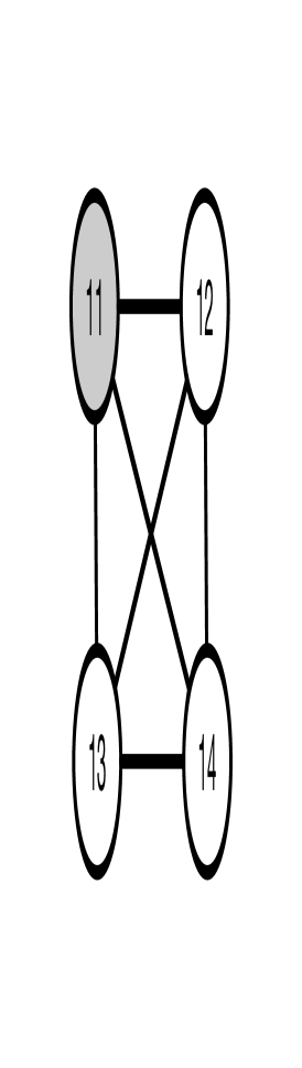
(a)

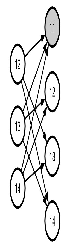
(b)

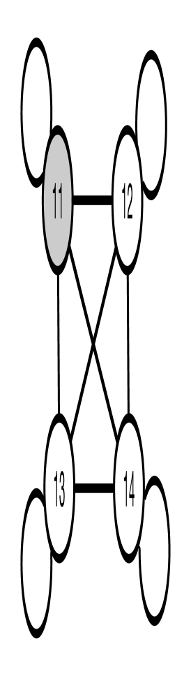
(c)

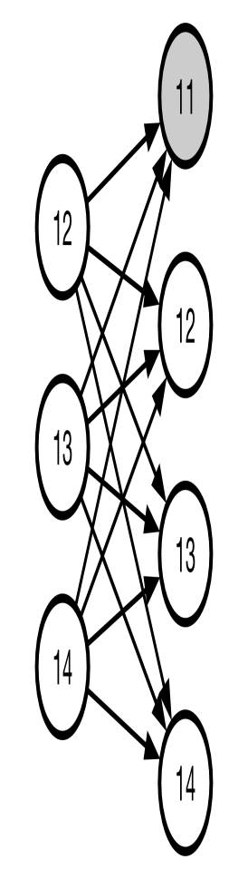
(d)

Figure 5: Network reporting when respondents are not included in their reports. (a) A single sibship. (b) The reporting network for the sibship in (a), when respondents are not included in reports. (c) The same sibship as (a) but with each sibling considered connected to herself. (d) The reporting network for the sibship in (c), when respondents are included in their reports.

Figure 5 illustrates the intuition behind the results we derive. The Figure shows sibships and reporting networks under the usual network reporting situation, where respondents are not included in their reports (panels a and b), and in an alternate situation, where respondents are included in their reports (panels c and d). Figure 5 illustrates the fact that whether or not the respondent includes herself in reports will only affect the visibility of siblings who are in the frame population: the visibility of node 11, which is dead (and thus not in the frame population) is unchanged under the two different scenarios. The other three nodes, on the other hand, have visibility 2 in panel b, when respondents are not included in their reports; and they have visibility 3 in panel d, when respondents are included in their reports.

.B.2 Expressions for individual visibility

Individual visibility estimation is based on separately adjusting for the visibility of each person being reported about. Below, in Appendix .F, we will use the expressions developed here to derive estimators for deaths and exposure using an individual visibility approach.

When the respondent is included in the reports

When the respondent is included in the reports, a reporting identity says that for person $i$ in sibship $\sigma[i]$,

$$v^{\prime}(i,\sigma[i]\cap F) =y^{\prime+}(\sigma[i]\cap F,i),$$ (18)

where we use the notation $v^{\prime}$ for visibilities when respondents include themselves in reports and $y^{\prime}$ for reports when respondents include themselves.

When reports are perfect, each sibling will be reported once for each member of the sibship on the frame population, so Equation 18 can be written as

$$v^{\prime}(i,\sigma[i]\cap F) =y^{\prime+}(\sigma[i]\cap F,i)$$ (19)

$$=d^{\prime}(\sigma[i]\cap F,i)$$ (if reporting is perfect)

$$=|\sigma\cap F|$$

$$=\bar{y}(\sigma[i]\cap F,\sigma[i]\cap F)+1$$

$$=y(j,F)+1 \text{for any $j\in\sigma[i]\cap F$}.$$

Equation 19 shows that, when analyzing reports about individual $i$ made by respondent $j$, $i$’s visibility under perfect reporting is $y(j,F)+1$.

When the respondent is not included in the reports

When the respondent does not include herself in her reports, a reporting identity says that, for population member $i$ in sibship $\sigma[i]$,

$$v(i,\sigma[i]\cap F) =y^{+}(\sigma[i]\cap F,i).$$ (20)

When reporting is perfect, $y^{+}(\sigma\cap F,i)$ is the number of $i$’s siblings who are on the frame population. Within a given sibship, this quantity will depend upon whether or not $i$ is herself on the frame population: in a sibship $\sigma$ with $|\sigma\cap F|$ members in $F$, there will be $|\sigma\cap F|$ siblings who can report a sibling $i$ who is not in $F$; on the other hand, when $i$ is in $F$, then $i$ counts towards the size of $|\sigma\cap F|$ and so there are $|\sigma\cap F|-1$ other siblings who can report $i$.

Mathematically, when reports are perfect, Equation 20 can be written as

$$v(i,\sigma\cap F) =y^{+}(\sigma\cap F,i)$$ (21)

$$=\begin{cases}|\sigma\cap F|&\text{if }i\notin F\\ |\sigma\cap F|-1&\text{if }\in F\end{cases}$$ (if reporting is perfect)

$$=\begin{cases}\bar{y}(\sigma\cap F,\sigma\cap F)+1&\text{if }i\notin F\\ \bar{y}(\sigma\cap F,\sigma\cap F)&\text{if }\in F\end{cases}$$

$$=\begin{cases}y(j,F)+1&\text{if }i\notin F\\ y(j,F)&\text{if }\in F\end{cases} \text{for any $j\in\sigma[i]\cap F$}.$$

Equation 21 shows that, when analyzing reports about individual $i$ made by respondent $j$, $i$’s visibility under perfect reporting is either $y(j,F)$ or $y(j,F)+1$, depending on whether $i$ is or is not in the frame population.

.B.3 Individual visibility estimands for mortality

.B.3.1 Individual visibility estimation including the respondent

When the respondent is included in the sibling reports, and when reports are perfect, Equation 19 shows that the visibility of each sibling is $\bar{y}(\sigma\cap F,\sigma\cap F)+1$. Note that when reports are perfect, $\bar{y}(\sigma\cap F,\sigma\cap F)=y(i,\sigma\cap F)$ and $y^{\prime}(i,\sigma\cap F)=y(i,\sigma\cap F)+1$ for all $i\in\sigma\cap F$.

Estimand for deaths using reports that include the respondent:

$$D^{\prime V}_{\alpha,ind} =\sum_{i\in F}\frac{y^{\prime}(i,D_{\alpha})}{y(i,F)+1}$$ (22)

$$=\sum_{i\in F}\frac{y^{\prime}(i,D_{\alpha})}{y^{\prime}(i,F)}$$

Estimand for exposure using reports that include the respondent:

$$N^{\prime V}_{\alpha,ind} =\sum_{i\in F}\frac{y^{\prime}(i,N_{\alpha})}{y(i,F)+1}$$ (23)

$$=\sum_{i\in F}\frac{y^{\prime}(i,N_{\alpha})}{y^{\prime}(i,F)}$$

Estimand for the death rate using reports that include the respondent:

$$M^{\prime V}_{\alpha,ind} =\frac{D^{\prime V}_{\alpha,ind}}{N^{\prime V}_{\alpha,ind}}$$ (24)

$$=\frac{\sum_{i\in F}\frac{y^{\prime}(i,D_{\alpha})}{y^{\prime}(i,F)}}{\sum_{i\in F}\frac{y^{\prime}(i,N_{\alpha})}{y^{\prime}(i,F)}}$$

.B.3.2 Individual visibility estimands not including the respondent

When the respondent does not include herself in reports about deaths and exposure, and when reports are perfect, Equation 21 shows that the visibility of a member $i$ of a sibship $\sigma$ reported by respondent $j\in\sigma[i]\cap F$ is given by:

$$v(i,\sigma\cap F) =\begin{cases}|\sigma\cap F|=\bar{y}(\sigma\cap F,\sigma\cap F)+1&\text{if }i\notin F\\ |\sigma\cap F|-1=\bar{y}(\sigma\cap F,\sigma\cap F)&\text{if }\in F\end{cases} \text{(if reporting is perfect)}.$$

Since $\bar{y}(\sigma\cap F,\sigma\cap F)=y(j,\sigma\cap F)$ for each $j\in\sigma\cap F$ when reports are perfect, we use the reported quantities $y(j,\sigma\cap F)$ and $1+y(j,\sigma\cap F)$ to estimate visibilities for siblings in the frame and not in the frame, respectively.

Estimand for deaths using reports that don’t include the respondent:

$$D^{V}_{\alpha,ind} =\sum_{i\in F}\left[\underbrace{\frac{y(i,D_{\alpha}\cap F)}{y(i,F)}}_{\text{$D_{\alpha}\cap F=\emptyset$}}+\underbrace{\frac{y(i,D_{\alpha}-F)}{y(i,F)+1}}_{\text{siblings not in $F$}}\right]$$ (when reports are perfect) (25)

$$=\sum_{i\in F}\frac{y(i,D_{\alpha})}{y(i,F)+1}.$$

In going from the first line to the second, we make use of the fact that deaths cannot be on the frame population, so that $y(i,D_{\alpha}\cap F)=0$ for all $i$, and so $y(i,D_{\alpha})=y(i,D_{\alpha}-F)$ for all $i$.

Estimand for exposure using reports that don’t include the respondent:

$$N^{V}_{\alpha,ind} =\sum_{i\in F}\left[\underbrace{\frac{y(i,N_{\alpha}\cap F)}{y(i,F)}}_{\text{siblings in $F$}}+\underbrace{\frac{y(i,N_{\alpha}-F)}{y(i,F)+1}}_{\text{siblings not in $F$}}\right] \text{(when reports are perfect)}.$$ (26)

Estimand for the death rate using reports that don’t include the respondent:

The estimand for the death rate is the ratio of the estimand for the number of deaths and the estimand for the exposure:

$$M^{V}_{\alpha,ind} =\frac{\sum_{i\in F}\frac{y(i,D_{\alpha})}{y(i,F)+1}.}{\sum_{i\in F}\left[\frac{y(i,N_{\alpha}\cap F)}{y(i,F)}+\frac{y(i,N_{\alpha}-F)}{y(i,F)+1}\right].}$$ (27)

.B.4 Expressions for aggregate visibility

Aggregate visibility estimation is based on adjusting for the average visibility of the people being reported about. In this section, we develop expressions for the average visibility of siblings who are in some group $A\subset U$. By deriving results for a general group $A$, we will obtain expressions that can be readily used for both deaths and exposure (see Appendix .E).

When the respondent is included in the reports

When reports include the respondent, the average visibility of siblings in a group $A$ is:

$$\bar{v}^{\prime}(A,F) =|A|^{-1}\sum_{i\in A}v^{\prime}(i,F)$$ (28)

$$=|A|^{-1}\sum_{i\in A}y^{\prime+}(F,i).$$

When reporting is perfect, this becomes

$$\bar{v}^{\prime}(A,F) =|A|^{-1}\sum_{i\in A}y^{\prime+}(F,i)$$ (29)

$$=|A|^{-1}\sum_{i\in A}\left[\bar{y}(\sigma[i]\cap F,\sigma[i]\cap F)+1\right]$$ (if reporting is perfect)

$$=|A|^{-1}\sum_{\sigma\in\Sigma}\sum_{i\in\sigma\cap A}|\sigma\cap F|$$

$$=|A|^{-1}\sum_{\sigma\in\Sigma}\left[|\sigma\cap A|~{}|\sigma\cap F|\right]$$

$$=\sum_{\sigma\in\Sigma}\underbrace{\frac{|\sigma\cap A|}{|A|}}_{\begin{subarray}{c}\text{fraction of}\\ \text{$A$ in}\\ \text{in sibship $\sigma$}\end{subarray}}\underbrace{|\sigma\cap F|}_{\begin{subarray}{c}\text{\# sibship}\\ \text{members}\\ \text{on frame}\end{subarray}}.$$

Equation 29 shows that the visibility can be expressed as a weighted average of the number of siblings on the frame across all of the sibships in the population, where the weights are given by the proportion of $A$ in each sibship.

Unlike the results for individual visibility estimation, we see no way to convert Equation 29 into a sample-based estimator for visibility. As we will see below, when estimating a death rate using an aggregate visibility estimator, we will take the ratio of two aggregate visibility estimators. Under the assumption that the visibility of the numerator and denominator are the same the visibilities will cancel, so that aggregate visibility does not need to be directly estimated.

When the respondent is not included in the reports

When reports do not include the respondent, the average visibility of siblings in a group $A$ is:

$$\bar{v}(A,F) =|A|^{-1}\sum_{i\in A}v(i,F)$$

$$=|A|^{-1}\sum_{i\in A}y^{+}(F,i)$$

$$=|A|^{-1}\sum_{\sigma\in\Sigma}\sum_{i\in\sigma\cap A}y^{+}(F,i).$$

When reporting is perfect, this becomes

$$\bar{v}(A,F) =|A|^{-1}\sum_{\sigma\in\Sigma}\sum_{i\in\sigma\cap A}y^{+}(F,i)$$ (30)

$$=|A|^{-1}\sum_{\sigma\in\Sigma}\left[\underbrace{\sum_{i\in\sigma\cap A\cap F}\bar{y}(\sigma[i]\cap F,\sigma[i]\cap F)}_{\text{members of $A$ on frame}}+\underbrace{\sum_{i\in\sigma\cap A-F}(\bar{y}(\sigma[i]\cap F,\sigma[i]\cap F)+1)}_{\text{members of $A$ not on frame}}\right]$$ (if reporting is perfect)

$$=|A|^{-1}\sum_{\sigma\in\Sigma}\left[\sum_{i\in\sigma\cap A}\bar{y}(\sigma[i]\cap F,\sigma[i]\cap F)+\sum_{i\in\sigma\cap A-F}1\right]$$

$$=\sum_{\sigma\in\Sigma}\frac{|\sigma\cap A|}{|A|}\bar{y}(\sigma\cap F,\sigma\cap F)+\sum_{\sigma\in\Sigma}\frac{|\sigma\cap A-F|}{|A|}$$

$$=\sum_{\sigma\in\Sigma}\frac{|\sigma\cap A|}{|A|}(|\sigma\cap F|-1)+\sum_{\sigma\in\Sigma}\frac{|\sigma\cap A-F|}{|A|}$$

$$=\sum_{\sigma\in\Sigma}\left[\frac{|\sigma\cap A|}{|A|}|\sigma\cap F|-\frac{|\sigma\cap A|}{|A|}+\frac{|\sigma\cap A-F|}{|A|}\right]$$

$$=\sum_{\sigma\in\Sigma}\frac{|\sigma\cap A|}{|A|}\left[|\sigma\cap F|-\frac{|\sigma\cap F\cap A|}{|\sigma\cap A|}\right].$$

Comparing Equation 30 to the analogous expression we derived for the situation where respondents do include themselves in reports (Equation 29), we find that the two expressions differ according to the second factor in the sum: when respondents include themselves in reports, this second factor is always the number of siblings in the frame population, $|\sigma\cap F|$; when respondents do not include themselves, this second factor is the number of siblings in the frame population minus the proportion of siblings in $A$ that is on the frame population, i.e., $|\sigma\cap F|-|\sigma\cap F\cap A|/|\sigma\cap A|$.

Note also that, by using the average visibility we derived for reports where respondents include themselves (Equation 29), we have an alternate way to write the result in Equation 30:

$$\bar{v}(A,F) =\sum_{\sigma\in\Sigma}\frac{|\sigma\cap A|}{|A|}\left[|\sigma\cap F|-\frac{|\sigma\cap F\cap A|}{|\sigma\cap A|}\right]$$ (31)

$$=\bar{v}^{\prime}(A,F)-\frac{|F\cap A|}{|A|}.$$

Equation 31 shows that the aggregate visibility when respondents are not included in reports is equal to the aggregate visibility when respondents are included in reports, minus the fraction of the set $A$ that is in the frame population.

.B.5 Aggregate visibility estimands for mortality

In Section .B.4, we saw that the expressions for the average visibility did not readily lend themselves to forming estimators. In the situation where we wish to estimate death rates, however, the condition that visibility is the same for deaths and for exposure leads to an estimator where the visibilities cancel, meaning that they do not have to be directly estimated. We can then investigate the sensitivity of estimated death rates to different visibilities as part of the broader sensitivity framework (Section .E).

For the estimands below, we write aggregate visibilities for a set $A$ as $\bar{v}(A,F)$ and $\bar{v}^{\prime}(A,F)$, bearing in mind that this cancellation will take place in the estimand for the death rate.

.B.5.1 Aggregate visibility estimands not including the respondent

Estimand for deaths using reports that don’t include the respondent

$$D^{V}_{\alpha,agg} =\frac{y_{F,D_{\alpha}}}{\bar{v}_{D_{\alpha},F}}.$$ (32)

Estimand for exposure using reports that don’t include the respondent

$$N^{V}_{\alpha,agg} =\frac{y_{F,N_{\alpha}}}{\bar{v}_{N_{\alpha},F}}.$$ (33)

Estimand for the death rate using reports that don’t include the respondent

$$M^{V}_{\alpha,agg} =\frac{D^{V}_{\alpha,agg}}{N^{V}_{\alpha,agg}}$$ (34)

$$=\frac{y_{F,D_{\alpha}}}{\bar{v}_{D_{\alpha},F}}~{}\frac{\bar{v}_{N_{\alpha},F}}{y_{F,N_{\alpha}}}$$

$$=\frac{y_{F,D_{\alpha}}}{y_{F,N_{\alpha}}}~{}\frac{\bar{v}_{N_{\alpha},F}}{\bar{v}_{D_{\alpha},F}}.$$

.B.5.2 Aggregate visibility estimands including the respondent

Estimand for deaths using reports that include the respondent

$$D^{\prime V}_{\alpha,agg} =\frac{y^{\prime}_{F,D_{\alpha}}}{\bar{v}^{\prime}_{D_{\alpha},F}}.$$ (35)

Estimand for exposure using reports that include the respondents

$$N^{\prime V}_{\alpha,agg} =\frac{y^{\prime}_{F,N_{\alpha}}}{\bar{v}^{\prime}_{N_{\alpha},F}}.$$ (36)

Estimand for the death rate using reports that include the respondent

$$M^{\prime V}_{\alpha,agg} =\frac{D^{\prime V}_{\alpha,agg}}{N^{\prime V}_{\alpha,agg}}$$ (37)

$$=\frac{y^{\prime}_{F,D_{\alpha}}}{\bar{v}^{\prime}_{D_{\alpha},F}}~{}\frac{\bar{v}^{\prime}_{N_{\alpha},F}}{y^{\prime}_{F,N_{\alpha}}}$$

$$=\frac{y^{\prime}_{F,D_{\alpha}}}{y^{\prime}_{F,N_{\alpha}}}~{}\frac{\bar{v}^{\prime}_{N_{\alpha},F}}{\bar{v}^{\prime}_{D_{\alpha},F}}.$$

Appendix .C Sensitivity to invisible deaths

Reports about siblings can only tell us about the visible population – i.e., the group of people who have siblings on the frame population who can provide information about their survival. In this Appendix, we develop expressions that relate the death rate in the visible population to the death rate in the entire population. This expression will help researchers understand how different death rates in the visible population can be expected to be from death rates in the entire population.

In order to analyze the sensitivity of sibling survival estimates to invisible deaths, we need to develop notation that can be used to distinguish between visible and invisible deaths. For a demographic group $\alpha$ (for example, women aged 15-25 in 2018), let

$$p^{V}_{D_{\alpha}} =\frac{D^{V}_{\alpha}}{D^{V}_{\alpha}+D^{I}_{\alpha}},$$ be the fraction of deaths that is visible; (38)

$$p^{V}_{N_{\alpha}} =\frac{N^{V}_{\alpha}}{N^{V}_{\alpha}+N^{I}_{\alpha}},$$ be the fraction of exposure that is visible.

We define analogous quantities for the fraction of deaths and exposure that is invisible, $p^{I}_{D_{\alpha}}$ and $p^{I}_{N_{\alpha}}$.

Note that

$$\frac{p^{V}_{D_{\alpha}}}{p^{V}_{N_{\alpha}}} =\frac{D^{V}_{\alpha}}{D^{V}_{\alpha}+D^{I}_{\alpha}}\times\frac{N^{V}_{\alpha}+N^{I}_{\alpha}}{N^{V}_{\alpha}}$$ (39)

$$=\frac{M^{V}_{\alpha}}{M_{\alpha}}.$$

Thus, the ratio of the fraction of deaths that is visible to the fraction of exposure that is visible is equal to the ratio of the visible death rate to the total death rate.

Result .H.2 shows that the total death rate $M_{\alpha}$ can be understood as a weighted harmonic mean of the invisible death rate $M^{I}_{\alpha}$ and the visible death rate $M^{V}_{\alpha}$, where the weights are given by the number of visible and invisible deaths. We now use this insight to develop Result .C.1, which helps us understand the formal relationship between the invisible death rate, the visible death rate, and the total death rate.

Result .C.1.

Suppose that, for a demographic group $\alpha$, the invisible death rate ($M^{I}_{\alpha}$) and the visible death rate ($M^{V}_{\alpha}$) differ by a factor of $K$, so that

$$M^{I}_{\alpha}=KM^{V}_{\alpha}$$ (40)

for $K>0$. Then

$$M_{\alpha} =M_{\alpha}^{V}\left[\frac{K}{p^{I}_{D_{\alpha}}+K(1-p^{I}_{D_{\alpha}})}\right],$$ (41)

where $p^{I}_{D_{\alpha}}$ is the proportion of deaths that is invisible.

Proof.

Using the fact that $M_{\alpha}$ is the weighted harmonic mean of $M^{I}_{\alpha}$ and $M^{V}_{\alpha}$, we find

$$M_{\alpha} =\left[\frac{p^{I}_{D_{\alpha}}}{M^{I}_{\alpha}}+\frac{p^{V}_{D_{\alpha}}}{M^{V}_{\alpha}}\right]^{-1}$$

$$=\left[\frac{p^{I}_{D_{\alpha}}}{KM^{V}_{\alpha}}+\frac{p^{V}_{D_{\alpha}}}{M^{V}_{\alpha}}\right]^{-1}$$

$$=\left[\frac{p^{I}_{D_{\alpha}}+Kp^{V}_{D_{\alpha}}}{KM^{V}_{\alpha}}\right]^{-1}$$

$$=M_{\alpha}^{V}\left[\frac{K}{p^{I}_{D_{\alpha}}+Kp^{V}_{D_{\alpha}}}\right]$$

$$=M_{\alpha}^{V}\left[\frac{K}{p^{I}_{D_{\alpha}}+K(1-p^{I}_{D_{\alpha}})}\right].$$

∎

Result .C.1 reveals that there is a relationship between between $K$, the difference between the visible and invisible death rates, and $p^{I}_{D_{\alpha}}$, which is related to the number of invisible deaths relative to the number of visible deaths. Equation 41 shows that

• when $K=1$, $M_{\alpha}^{V}=M_{\alpha}$

• when $p^{I}_{D_{\alpha}}=0$, $p^{V}_{D_{\alpha}}=1$ and so $M_{\alpha}^{V}=M_{\alpha}$

It can also be helpful to use Result .C.1 to obtain an expression for the relative error that would follow from using the visible death rate $M^{V}_{\alpha}$ as an estimate of the total death rate $M_{\alpha}$:

$$\frac{M^{V}_{\alpha}-M_{\alpha}}{M_{\alpha}} =\frac{M^{V}_{\alpha}}{M_{\alpha}}-1$$ (42)

$$=\frac{p^{V}_{D_{\alpha}}+K(1-p^{V}_{D_{\alpha}})}{K}-1$$

$$=p^{I}_{D_{\alpha}}\left(\frac{1-K}{K}\right).$$

In order to further develop intuition about how large we might expect biases due to invisible deaths to be, we can investigate different scenarios. For example, suppose that 10% of deaths are invisible, and the death rate is 20% higher among the invisible population than among the visible population. Then $K=1.2$, $p^{I}_{D_{\alpha}}=0.1$, and the relative error calculated from Equation 42 is about -.017; in other words, in this scenario, death rate estimates based on the visible population alone will be too low by about 1.7 percent.

Figure 6 illustrates this relative error for a range of values of $K$ and $p^{I}_{D_{\alpha}}$.

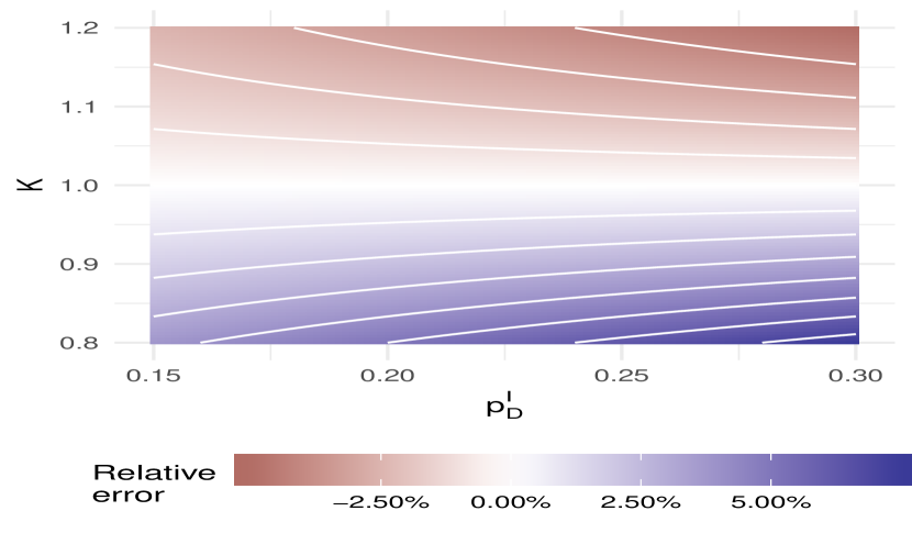
Figure 6: Illustration of the relative error in using the visible death rate $M^{V}$ as an estimate for the total death rate $M$. The proportion of deaths that is invisible, $p^{I}_{D_{\alpha}}$, varies along the x axis; the relationship between the visible and invisible death rates, captured by the parameter $K$ (Equation 40), varies along the y axis. The colors show the percentage relative error; so if 20% of deaths are invisible ($p^{I}_{D_{\alpha}}=0.2$) and the invisible death rate is 10% higher than the visible death rate ($K=1.1$), the relative error is about 2 percent. Relative error increases as $K$ gets farther away from 1 and as $p^{V}_{D_{\alpha}}$ increases.

Next, Result .C.2 provides a second expression that analyzes the formal relationship between the invisible death rate, the visible death rate, and the total death rate; this second result is parameterized in terms of $p^{I}_{N_{\alpha}}$, the proportion of exposure that is invisible. This is the relationship used in the main text.

Result .C.2.

Suppose that, for a demographic group $\alpha$, the invisible death rate ($M^{I}_{\alpha}$) and the visible death rate ($M^{V}_{\alpha}$) differ by a factor of $K$, so that

$$M^{I}_{\alpha}=KM^{V}_{\alpha}$$ (43)

for $K>0$. Then

$$M_{\alpha} =M_{\alpha}^{V}\left[1+p^{I}_{N_{\alpha}}(K-1)\right],$$ (44)

where $p^{I}_{N_{\alpha}}$ is the proportion of exposure that is invisible.

Proof.

Using the fact that $M_{\alpha}$ is the weighted arithmetic mean of $M^{I}_{\alpha}$ and $M^{V}_{\alpha}$, we find

$$M_{\alpha} =p^{V}_{N_{\alpha}}M^{V}_{\alpha}+p^{I}_{N_{\alpha}}M^{I}_{\alpha}$$

$$=(1-p^{I}_{N_{\alpha}})M^{V}_{\alpha}+p^{I}_{N_{\alpha}}KM^{V}_{\alpha}$$

$$=M^{V}_{\alpha}-M^{V}_{\alpha}p^{I}_{N_{\alpha}}+Kp^{I}_{N_{\alpha}}M^{V}_{\alpha}$$

$$=M^{V}_{\alpha}\left[1+p^{I}_{N_{\alpha}}(K-1)\right].$$

∎

Again, it can be helpful to use Result .C.2 to obtain an expression for the relative error that would follow from using the visible death rate $M^{V}_{\alpha}$ as an estimate of the total death rate $M_{\alpha}$:

$$\frac{M^{V}_{\alpha}-M_{\alpha}}{M_{\alpha}} =\frac{M^{V}_{\alpha}}{M_{\alpha}}-1$$ (45)

$$=\frac{1}{1+p^{I}_{N_{\alpha}}(K-1)}-1$$

$$=\frac{p^{I}_{N_{\alpha}}(1-K)}{1-p^{I}_{N_{\alpha}}(1-K)}.$$

We can further develop intuition about how large we might expect biases due to invisible deaths to be, we can investigate different scenarios. For example, suppose that 10% of exposure is invisible, and the death rate is 20% higher among the invisible population than among the visible population. Then $K=1.2$, $p^{I}_{N_{\alpha}}=0.1$, and the relative error from Equation 45 is about -0.019; in other words, in this scenario, death rate estimates based on the visible population alone will be too low by about 1.9 percent.

Figure 3b illustrates this second expression for the relative error over a range of values of $K$ and $p^{I}_{N_{\alpha}}$.

Appendix .D Sampling

In Appendix .B, we developed several estimands based on sibling reports. These estimands describe quantities that could be estimated from a census of the frame population. In practice, researchers do not have a census of the frame population, but rather a sample from the frame population. This section develops some results that will be helpful in understanding how to develop sample-based estimators for the estimands in Appendix .B.

.D.1 Sampling setup

We use the design-based sampling framework described in Sarndal, Swensson, and Wretman (2003), repeating a few key definitions here for convenience. We assume we have a probability sample $s$ from a frame population $F$; common frame populations include all adults, all adults aged 15-59, and in many DHS surveys, all women aged 15-59. The random variable $I_{i}$ takes the value 1 when $i\in F$ is included in the sample, and 0 otherwise. Each $i\in F$ has a nonzero probability of inclusion $\pi_{i}=\mathbb{E}[I_{i}]$ and the sampling weights are given by $w_{i}=\frac{1}{\pi_{i}}$.

Suppose some quantity $y_{i}$ is defined for every $i\in F$. Then the Horvitz Thompson estimator for the population total $Y=\sum_{i\in F}y_{i}$ from a probability sample $s$ is given by

$$\widehat{Y}=\sum_{i\in s}w_{i}y_{i}.$$

Sarndal, Swensson, and Wretman (2003) shows that Horvitz-Thompson estimators are consistent and unbiased, a fact that will be useful below.

Result .D.1.

Suppose a Horvitz-Thompson estimator

$$\widehat{Y}^{\text{HT}}=\sum_{i\in s}w_{i}y_{i}$$

is design-unbiased for a total $Y$. Then $\widehat{Y}^{\text{HT}}$ is also (design) consistent for $Y$.

Proof.

This result follows from taking the sampling design to assign $\pi_{i}=1$ for all $i\in F$. We then have $s=F$ and $w_{i}=1$ for all $i$. Since the estimator is unbiased, design consistency follows.

∎

Next, we state a Result that is helpful when devising estimators that are ratios of other estimators.

Result .D.2.

Suppose that $\widehat{y}_{1},\dots,\widehat{y}_{n}$ are estimators that are consistent and unbiased for $Y_{1},\dots,Y_{n}$ respectively. Then the compound ratio estimator

$$\widehat{R}=\frac{\widehat{y}_{1}\dots\widehat{y}_{k}}{\widehat{y}_{k+1}\dots\widehat{y}_{n}}.$$

is consistent and essentially unbiased for $R=(Y_{1}\dots Y_{k})/(Y_{k+1}\dots Y_{n})$.

Proof.

See Rao and Pereira (1968), Wolter (2007) (pg. 233), and Feehan and Salganik (2016a) for more details.

∎

The references that derive the compound ratio estimator in Result .D.2 show that, technically, the estimator is biased. However, the bias has been shown to be of order $O(n^{-1})$; that is, the bias goes to 0 as the sample size $n\to\infty$. Further, Feehan and Salganik (2016a) investigated compound ratio bias in network reporting estimators and found suggestive evidence that it is likely to be very small. This finding is consistent with the literature on ratio estimators, which has revealed that bias is often very small. Thus, in these technical results, we refer to estimators whose only bias arises from being compound ratios – i.e., whose bias is of order $O(n^{-1})$ – as essentially unbiased.

.D.2 Adjusting for visibility in samples

In this section, we briefly state key results that explain which conditions are required for individual and aggregate visibility estimators to be consistent and unbiased. More detailed derivations of these results can be found elsewhere.

Individual visibility estimation from a probability sample

Definition .D.1.

The individual visibility estimator for a total $\boldsymbol{Y}=\sum_{i\in U}y_{i}$ is defined to be

$$\widehat{Y}^{\text{ind}}=\sum_{i\in s}w_{i}\sum_{j\sim i}\frac{y_{j}}{v_{j,F}},$$ (46)

where $j\sim i$ indexes the neighbors $j$ of respondent $i$, $w_{i}$ is the design weight for respondent $i$, and $v_{j,F}$ is the visibility of person $j$ to the frame population $F$. In the situation where there are no errors in reporting, the visibility $v_{j,F}$ has also been called the multiplicity of person $j$ (Sirken 1970).

Result .D.3.

Suppose that there are no false positive reports. The individual visibility estimator is consistent and unbiased for the total $\boldsymbol{Y}$.

Proof.

First, we show that the estimator is unbiased. If $\pi_{i}$ is $i$’s probability of inclusion under the sampling design, then the design weights are $w_{i}=\frac{1}{\pi_{i}}$. Thus, we have

$$\widehat{\boldsymbol{Y}}^{\text{ind}} =\sum_{i\in s}\frac{1}{\pi_{i}}\sum_{j\sim i}\frac{y_{j}}{v_{j,F}}$$

$$\Longleftrightarrow\mathbb{E}[\widehat{\boldsymbol{Y}}^{\text{ind}}] =\sum_{i\in F}\mathbb{E}[I_{i}]\frac{1}{\pi_{i}}\sum_{j\sim i}\frac{y_{j}}{v_{j,F}}$$

$$=\sum_{i\in F}\sum_{j\sim i}\frac{y_{j}}{v_{j,F}}$$

$$=\sum_{l\in F}v_{l,F}\frac{y_{l}}{v_{l,F}}$$

$$=\sum_{l\in F}y_{l}.$$

The last step follows because, as long as there are no false positive reports, in a census of $F$, each unit $j$ appears once for each time it is visible to $F$; that is, $v_{j,F}=y_{F,j}$ (see Feehan and Salganik (2016a) for details).

Note that the derivation above reveals that the individual visibility estimator can be written as a Horvitz-Thompson estimator (Thompson 2002; Sirken 1970): to see how, define $z_{i}=\sum_{j\sim i}\frac{y_{j}}{v_{j,F}}$ for all $i\in F$. The individual visibility estimator in Equation 46 then becomes $\widehat{Y}=\sum_{i\in s}w_{i}z_{i}$. Since $\widehat{\boldsymbol{Y}}^{\text{ind}}$ can be written as a Horvitz-Thompson estimator, Result .D.1 shows that unbiasedness implies consistency.

∎

Good references for individual visibility estimators include Sirken (1970) and Lavallee (2007).

Aggregate visibility estimation from a probability sample

Definition .D.2.

The aggregate visibility estimator for a total $\boldsymbol{Y}=\sum_{i\in U}y_{i}$ is defined to be

$$\widehat{Y}^{\text{agg}}=\frac{\sum_{i\in s}w_{i}\sum_{j\sim i}y_{j}}{\widehat{\bar{v}}_{Y,F}},$$

where $\bar{v}_{Y,F}=N^{-1}\sum_{l\in U}v_{l,F}$ is the average of the individual visibilities of each person who could be reported about in a census of $F$.

The network scale-up estimator, the network survival estimator, and related approaches are examples of estimators based on the idea of aggregate visibility (Bernard et al. 1989; Feehan and Salganik 2016a; Feehan, Mahy, and Salganik 2017).

Result .D.4.

Suppose that there are no false positive reports. Then the aggregate visibility estimator is consistent and essentially unbiased for the total $\boldsymbol{Y}$.

Proof.

See Feehan and Salganik (2016a).

∎

Appendix .E Estimating death rates using aggregate visibility

This section presents results for death rate estimators that adjust for visibility at the aggregate level; that is, the sum of reported connections to siblings across respondents is adjusted for using the average visibility of the reported siblings.

Section .B.4 showed that there is no one obvious way to estimate the aggregate visibility of deaths or exposure using data collected from the sibling histories. However, if the visibility of deaths is the same as the visibility of exposure, then the death rate can be estimated without directly estimating the visibility of deaths or exposure, since these two quantities will cancel. This condition is analogous to the requirement, discussed at length in the sibling survival literature, that there be no correlation between sibship size and mortality. We suggest that researchers assess the sensitivity of aggregate visibility estimators to this condition using the sensitivity framework we develop below.

We will first provide an estimator that is based on excluding information about the survey respondents and only using reports about respondents’ siblings. We will see that this approach produces an estimator that is essentially the one recommended in the DHS program’s official documentation (Rutstein and Guillermo Rojas 2006, pg. 156) and by other researchers (e.g., Masquelier 2013). An additional estimator, based on including information about the survey respondents, turns out to be very similar, and follows as a Corollary of the derivation of the without-respondent estimator.

The relationship derived in Equation 34 suggests

$$\widehat{M}^{V}_{\alpha} =\frac{\widehat{D}^{V}_{\alpha}}{\widehat{N}^{V}_{\alpha}}$$ (47)

$$=\frac{\sum_{i\in s}w_{i}~{}y(i,D_{\alpha})}{\sum_{i\in s}w_{i}~{}y(i,N_{\alpha})}.$$

Equation 47 is based on the idea that we can plug in sample-based aggregate visibility estimators for the number of siblings who died and the number of siblings who contribute exposure. Result .E.1 formally states the conditions are required for the estimator to produce consistent and unbiased estimates for the visible death rate.

Result .E.1.

(Aggregate visibility estimation for death rates) Suppose we have a probability sample $s\subset F$ and the associated weights $w_{i}$ for all $i\in s$. Suppose that, in aggregate, there are no false positive reports about deaths or exposure, so that $y(F,D_{\alpha})=y^{+}(F,D_{\alpha})$ and $y(F,N_{\alpha})=y^{+}(F,N_{\alpha})$. Suppose also that the visibility of deaths and exposure to the frame population are the same, and nonzero, so that $\bar{v}(D_{\alpha},F)=\bar{v}(N_{\alpha},F)>0$. Then

$$\widehat{M}^{V} =\frac{\widehat{y}(F,D_{\alpha})}{\widehat{y}(F,N_{\alpha})}$$ (48)

$$=\frac{\sum_{i\in s}w_{i}~{}y(i,D_{\alpha})}{\sum_{i\in s}w_{i}~{}y(i,N_{\alpha})}$$

is consistent and essentially unbiased for $M^{V}_{\alpha}=\frac{D^{V}_{\alpha}}{N^{V}_{\alpha}}$, where the exposure $N^{V}_{\alpha}$ is approximated by the number of visible people, living or dead, in group $\alpha$.

Proof.

The numerator and denominator are Horvitz-Thompson estimators, and are therefore consistent and unbiased for the population quantities $y(F,D_{\alpha})$ and $y(F,N_{\alpha})$. By Result .D.2, $\widehat{M}^{V}$ is then consistent and essentially unbiased for the estimand $\frac{y(F,D_{\alpha})}{y(F,N_{\alpha})}$, so it remains to show that this estimand is equal to the visible death rate. Using the fact that $\bar{v}(D_{\alpha},F)=\bar{v}(N_{\alpha},F)$, we have

$$\frac{y(F,D_{\alpha})}{y(F,N_{\alpha})}=\frac{y(F,D_{\alpha})}{y(F,N_{\alpha})}~{}\frac{\bar{v}(N_{\alpha},F)}{\bar{v}(D_{\alpha},F)}.$$

Since there are no false positive reports about death or exposure, we have

$$\frac{y(F,D_{\alpha})}{y(F,N_{\alpha})}~{}\frac{\bar{v}(N_{\alpha},F)}{\bar{v}(D_{\alpha},F)}=\frac{y^{+}(F,D_{\alpha})}{y^{+}(F,N_{\alpha})}~{}\frac{\bar{v}(N_{\alpha},F)}{\bar{v}(D_{\alpha},F)}.$$

By the aggregate reporting identity, $y^{+}(F,D_{\alpha})/\bar{v}(D_{\alpha},F)=D^{V}_{\alpha}$ and $y^{+}(F,N_{\alpha})/\bar{v}(N_{\alpha},F)=N^{V}_{\alpha}$. Therefore, we have

$$\frac{y^{+}(F,D_{\alpha})}{y^{+}(F,N_{\alpha})}~{}\frac{\bar{v}(N_{\alpha},F)}{\bar{v}(D_{\alpha},F)}=\frac{D^{V}_{\alpha}}{N^{V}_{\alpha}}=M^{V}_{\alpha}.$$

∎

To recap, Result .E.1 shows that the estimator for visible death rates relies on the important condition that the visibility of deaths is the same as the visibility of exposure. This requirement does not mean that reports have to be perfectly accurate; in particular, omitting siblings will only cause a problem if it happens at a different rate for dead siblings than it does for living siblings. We discuss this issue in more detail when we develop the sensitivity analysis framework, below.

The Corollary below says that, when respondents are included in reports, then an analogous set of conditions to the ones required by Result .E.1 will allow consistent and unbiased estimation of the death rate.  

Corollary .E.1.

(Aggregate visibility estimation for death rates when respondents are included in reports). Result .E.1 holds under analogous conditions when reports include the respondents. Specifically, suppose we have a probability sample $s\subset F$ and the associated weights $w_{i}$ for all $i\in s$. Suppose that there are no false positive reports about deaths or exposure, so that $y^{\prime}(F,D_{\alpha})=y^{\prime+}(F,D_{\alpha})$ and $y^{\prime}(F,N_{\alpha})=y^{\prime+}(F,N_{\alpha})$. Suppose also that the visibility of deaths and exposure to the frame population are the same, and nonzero, so that $\bar{v}^{\prime}(D_{\alpha},F)=\bar{v}^{\prime}(N_{\alpha},F)>0$. Then

$$\widehat{M}^{\prime V} =\frac{\widehat{y}^{\prime}(F,D_{\alpha})}{\widehat{y}^{\prime}(F,N_{\alpha})}$$ (49)

$$=\frac{\sum_{i\in s}w_{i}~{}y^{\prime}(i,D_{\alpha})}{\sum_{i\in s}w_{i}~{}y^{\prime}(i,N_{\alpha})}$$

is consistent and essentially unbiased for $M^{\prime V}_{\alpha}=\frac{D^{\prime V}_{\alpha}}{N^{\prime V}_{\alpha}}$, where the exposure $N^{V}_{\alpha}$ is approximated by the number of visible people, living or dead, in group $\alpha$.

Proof.

The proof follows the same steps as the proof of Result .E.1.

∎

It is important to note that the aggregate visibility estimator based on not including information about respondents (Result .E.1) is consistent and unbiased for a visible death rate $M^{V}_{\alpha}$, and that the aggregate visibility estimator based on including information about respondents (Corollary .E.1) is consistent and unbiased for a different visible death rate $M^{\prime V}_{\alpha}$. In other words, the definition of the visible and invisible populations will be affected by whether or not respondents are included in the sibling reports. We analyze this issue in more detail in Appendix .G.1.

Sensitivity of the aggregate visibility death rate estimator

We now turn to the sensitivity of the aggregate visibility death rate estimator to the various conditions it relies upon. Our approach is to introduce several quantities, called adjustment factors, that capture the degree to which the conditions the estimator relies upon are satisfied. These adjustment factors will be equal to 1 under ideal conditions, and will be different from 1 when a condition required by the death rate estimator is not satisfied. Our approach is closely related to other network reporting analyses, including Feehan and Salganik (2016a) and Feehan, Mahy, and Salganik (2017).

We consider here the case where respondents are not included in reports; however, an analogous sensitivity expression would result from extended our approach to the case where respondents are included in sibling reports.

The first adjustment factor is the true positive rate for reports about visible deaths, $\tau(F,D_{\alpha})$; it is defined as

$$\tau(F,D_{\alpha})=\frac{\text{average \# times a visible death in $\alpha$ would be reported by someone in $F$}}{\text{average number of connections a visible death in $\alpha$ has to $F$}}=\frac{\bar{v}(D^{V}_{\alpha},F)}{\bar{d}(D^{V}_{\alpha},F)}.$$ (50)

Note that we can also write $\tau(F,D_{\alpha})=\frac{\bar{y}^{+}(F,D_{\alpha})}{\bar{d}(F,D^{V}_{\alpha})}$, since $v(D^{V}_{\alpha},F)=y^{+}(F,D_{\alpha})$.

The second adjustment factor is the precision for reports about visible deaths, $\eta(F,D_{\alpha})$; it is defined as

$$\eta(F,D_{\alpha})=\frac{\text{\# of reported connections from $F$ to $D_{\alpha}$ that actually lead to $D_{\alpha}$}}{\text{\# of reported connections from $F$ to $D_{\alpha}$}}=\frac{y^{+}(F,D_{\alpha})}{y(F,D_{\alpha})}.$$ (51)

We define analogous adjustment factors $\tau(F,N_{\alpha})$ and $\eta(F,N_{\alpha})$ for $F$’s reports about siblings’ exposure.

We can use the adjustment factors introduced in the previous section to decompose the aggregate visibility sibling survival estimator as

$$M_{\alpha} =\frac{D_{\alpha}}{N_{\alpha}}$$ (52)

$$=\frac{D^{V}_{\alpha}}{N^{V}_{\alpha}}\times\frac{p^{V}_{N_{\alpha}}}{p^{V}_{D_{\alpha}}}$$

$$=\frac{D^{V}_{\alpha}}{N^{V}_{\alpha}}\times\frac{M_{\alpha}}{M^{V}_{\alpha}}$$

$$=\frac{y_{F,D_{\alpha}}}{y_{F,N_{\alpha}}}\times\frac{\bar{d}^{V}(N_{\alpha},F)}{\bar{d}^{V}(D_{\alpha},F)}\times\frac{\eta(F,D_{\alpha})}{\eta(F,N_{\alpha})}\times\frac{\tau(F,N_{\alpha})}{\tau(F,D_{\alpha})}\times\frac{M_{\alpha}}{M^{V}_{\alpha}}.$$

In order to simplify the eventual framework, let us introduce two quantities that capture net reporting about deaths and about exposure:

$$\gamma(F,D_{\alpha})=\frac{\tau(F,D_{\alpha})}{\eta(F,D_{\alpha})},$$

and

$$\gamma(F,N_{\alpha})=\frac{\tau(F,N_{\alpha})}{\eta(F,N_{\alpha})}.$$

The final step is to incorporate the expression for sensitivity to invisible siblings. Let the visible and invisible death rates differ by a factor $K$ so that $M_{\alpha}^{I}=KM_{\alpha}^{V}$. Equation 41 then tells us that

$$\frac{M^{V}_{\alpha}}{M_{\alpha}}=\frac{p^{V}_{D_{\alpha}}+K(1-p^{V}_{D_{\alpha}})}{K}.$$ (53)

Combining Equation 41 and Equation 52, and substituting $\gamma(F,D_{\alpha})$ and $\gamma(F,N_{\alpha})$, we obtain an expression that relates the aggregate visibility estimand to the true death rate:

$$M_{\alpha}=\underbrace{\frac{y(F,D_{\alpha})}{y(F,N_{\alpha})}}_{\begin{subarray}{c}\text{aggregate}\\ \text{mulitiplicity}\\ \text{estimand}\end{subarray}}\times\underbrace{\frac{\bar{d}^{V}(N_{\alpha},F)}{\bar{d}^{V}(D_{\alpha},F)}}_{\begin{subarray}{c}\text{degree}\\ \text{ratio}\end{subarray}}\times\underbrace{\frac{\gamma(F,N_{\alpha})}{\gamma(F,D_{\alpha})}}_{\begin{subarray}{c}\text{reporting}\\ \text{accuracy}\end{subarray}}\times\underbrace{\left[\frac{K}{p^{I}_{D_{\alpha}}+K(1-p^{I}_{D_{\alpha}})}\right].}_{\begin{subarray}{c}\text{difference between}\\ \text{invisible and}\\ \text{visible}\\ \text{populations}\end{subarray}}$$ (54)

This decomposition relates the quantities we can observe or estimate from a survey— i.e., $y(F,D_{\alpha})$ and $y(F,N_{\alpha})$–to the quantity that we actually wish to estimate, i.e., $M_{\alpha}$.

The decomposition in Equation 54 produces two groups of factors that are the ratio of (i) an adjustment factor for deaths; and (ii) the same adjustment factor for exposure (for example, $\frac{\gamma(F,D_{\alpha})}{\gamma(F,N_{\alpha})}$). To the extent that reporting about deaths and reporting about exposure is similar, this is advantageous: these adjustment factors can cancel or counteract one another. Intuitively, Equation 52 reveals that the death rate estimator is quite robust to situations in which respondents’ reports are imperfect, but imperfect in similar ways for deaths and for people who didn’t die.

Equation 52 parameterizes the difference between the visible and visible populations in terms of $p^{D}_{D_{\alpha}}$, the proportion of deaths that is invisible. Researchers may prefer to parameterize this factor in terms of $p^{I}_{N_{\alpha}}$, the proportion of exposure that is invisible. In that case, Equation 52 becomes:

$$M_{\alpha}=\underbrace{\frac{y(F,D_{\alpha})}{y(F,N_{\alpha})}}_{\begin{subarray}{c}\text{aggregate}\\ \text{mulitiplicity}\\ \text{estimand}\end{subarray}}\times\underbrace{\frac{\bar{d}^{V}(N_{\alpha},F)}{\bar{d}^{V}(D_{\alpha},F)}}_{\begin{subarray}{c}\text{degree}\\ \text{ratio}\end{subarray}}\times\underbrace{\frac{\gamma(F,N_{\alpha})}{\gamma(F,D_{\alpha})}}_{\begin{subarray}{c}\text{reporting}\\ \text{accuracy}\end{subarray}}\times\underbrace{\left[1+p^{I}_{N_{\alpha}}(K-1)\right].}_{\begin{subarray}{c}\text{difference between}\\ \text{invisible and}\\ \text{visible}\\ \text{populations}\end{subarray}}$$ (55)

Appendix .F Estimating death rates using individual visibility

This section presents results for death rate estimators that adjust for visibility at the individual level; that is, each reported connection to a siblings is adjusted for using the visibility of that specific reported sibling.

First, we provide an estimator that is based on excluding information about the survey respondents and only using reports about respondents’ siblings.

Result .F.1.

(Individual visibility estimation for death rates) Suppose that reports are accurate at the individual level, so that $y(i,D_{\alpha})=d(i,D_{\alpha})$ and $y(i,N_{\alpha})=d(i,N_{\alpha})$. Then

$$\widehat{M}^{V} =\frac{\widehat{D_{\alpha}}}{\widehat{N_{\alpha}}}$$ (56)

$$=\frac{\sum_{i\in s}w_{i}\frac{y(i,D_{\alpha})}{y(i,F)+1}}{\sum_{i\in s}w_{i}\left[\frac{y(i,N_{\alpha}\cap F)}{y(i,F)}+\frac{y(i,N_{\alpha}-F)}{y(i,F)+1}\right]}$$

is consistent and essentially unbiased for $M^{V}_{\alpha}=\frac{D^{V}_{\alpha}}{N^{V}_{\alpha}}$, where the exposure $N^{V}_{\alpha}$ is approximated by the number of visible people, living or dead, in group $\alpha$.

Proof.

The numerator and denominator are Horvitz-Thompson estimators, and therefore

$$\sum_{i\in s}w_{i}\frac{y(i,D_{\alpha})}{y(i,F)+1} \longrightarrow\sum_{i\in F}\frac{y(i,D_{\alpha})}{y(i,F)+1}$$

$$=\sum_{i\in F}\frac{d(i,D_{\alpha})}{d(i,F)+1}$$ by the perfect reporting condition

$$=D^{V}_{\alpha}.$$ by the derivation in Equation 25

Similarly,

$$\sum_{i\in s}w_{i}\left[\frac{y(i,N_{\alpha}\cap F)}{y(i,F)}+\frac{y(i,N_{\alpha}-F)}{y(i,F)+1}\right] \longrightarrow\sum_{i\in F}\left[\frac{y(i,N_{\alpha}\cap F)}{y(i,F)}+\frac{y(i,N_{\alpha}-F)}{y(i,F)+1}\right]$$

$$=\sum_{i\in F}\left[\frac{d(i,N_{\alpha}\cap F)}{d(i,F)}+\frac{d(i,N_{\alpha}-F)}{d(i,F)+1}\right]$$ by perfect reporting condition

$$=N_{\alpha} \begin{subarray}{c}\text{by relationship in}\\ \text{Equation \ref{eq:ind-exposure-noresp}}\end{subarray}$$

Therefore, the numerator of Equation 57 is consistent and unbiased for the visible deaths, $D^{V}_{\alpha}$, and the denominator of Equation 57 is consistent and unbiased for the visible exposure $N^{V}_{\alpha}$. Result .D.2 then shows that the ratio of these two estimators, $\widehat{M}^{V}=\frac{\widehat{D}_{\alpha}}{\widehat{N}_{\alpha}}$ will be consistent and essentially unbiased for, $\frac{D^{V}_{\alpha}}{N^{V}_{\alpha}}$, the visible death rate.

∎

Result .F.1 applies in the situation where respondents are not included in the sibship reports. We now turn to a Corollary that addresses the situation where information about respondents is included in the sibship reports.

Corollary .F.1.

(Individual visibility estimation for death rates when respondents are included in reports) Result .F.1 holds under analogous conditions when reports include the respondents. Specifically, suppose we have a probability sample $s\subset F$ and the associated weights $w_{i}$ for all $i\in s$. Suppose that reports are accurate at the individual level, so that $y^{\prime}(i,D_{\alpha})=d^{\prime}(i,D_{\alpha})$ and $y^{\prime}(i,N_{\alpha})=d^{\prime}(i,N_{\alpha})$. Then

$$\widehat{M}^{\prime V} =\frac{\widehat{D^{\prime}_{\alpha}}}{\widehat{N^{\prime}_{\alpha}}}$$ (57)

$$=\frac{\sum_{i\in s}w_{i}\frac{y^{\prime}(i,D_{\alpha})}{y^{\prime}(i,F)}}{\sum_{i\in s}w_{i}\frac{y^{\prime}(i,N_{\alpha})}{y^{\prime}(i,F)}}$$

is consistent and essentially unbiased for $M^{\prime V}_{\alpha}=\frac{D^{\prime V}_{\alpha}}{N^{\prime V}_{\alpha}}$, where the exposure $N^{V}_{\alpha}$ is approximated by the number of visible people, living or dead, in group $\alpha$.

Proof.

The proof is essentially the same as the proof of Result .F.1; we repeat it here for clarity. The numerator and denominator are Horvitz-Thompson estimators, and therefore

$$\sum_{i\in s}w_{i}\frac{y^{\prime}(i,D_{\alpha})}{y^{\prime}(i,F)} \longrightarrow\sum_{i\in F}\frac{y^{\prime}(i,D_{\alpha})}{y^{\prime}(i,F)}$$

$$=\sum_{i\in F}\frac{d^{\prime}(i,D_{\alpha})}{d^{\prime}(i,F)}$$ by the perfect reporting condition

$$=D^{\prime V}_{\alpha}.$$ by the derivation in Equation 22

Similarly,

$$\sum_{i\in s}w_{i}\frac{y^{\prime}(i,N_{\alpha}}{y^{\prime}(i,F)} \longrightarrow\sum_{i\in F}\frac{y^{\prime}(i,N_{\alpha})}{y^{\prime}(i,F)}$$

$$=\sum_{i\in F}\frac{d^{\prime}(i,N_{\alpha})}{d^{\prime}(i,F)}$$ by perfect reporting condition

$$=N^{\prime}_{\alpha}. \begin{subarray}{c}\text{by derivation in}\\ \text{Equation \ref{eq:ind-exposure-withresp}}\end{subarray}$$

Therefore, the numerator of the estimator (Equation 57) is consistent and unbiased for the visible deaths, $D^{\prime V}_{\alpha}$, and the denominator of Equation 57 is consistent and unbiased for the visible exposure $N^{\prime V}_{\alpha}$. Result .D.2 then shows that the ratio of these two estimators, $\widehat{M}^{\prime V}=\frac{\widehat{D}^{\prime}_{\alpha}}{\widehat{N}^{\prime}_{\alpha}}$ will be consistent and essentially unbiased for, $\frac{D^{\prime V}_{\alpha}}{N^{\prime V}_{\alpha}}$, the visible death rate when respondents are included in reports.

∎

.F.1 Sensitivity of individual death rate estimator

Now we turn to an analysis of the sensitivity of the individual visibility estimator. We follow the same approach that we did for the aggregate visibility estimator: we introduce a series of adjustment factors that relate reports to the underlying sibship network. Using these adjustment factors, we develop expressions that show how reporting errors and other factors will affect estimated death rates.

Adjustment factors for deaths

We start by defining individual-level adjustment factors that will be useful in understanding how reporting errors can affect the individual estimator. For a particular respondent $i\in F$ in sibship $\sigma$, let

$$\tau(i,D_{\alpha}\cap\sigma)=\frac{\text{\# sibs $i$ reports having died in group $\alpha$ that actually died in group $\alpha$}}{\text{\# siblings of $i$ that actually died in group $\alpha$}}=\frac{y^{+}(i,D^{V}_{\alpha}\cap\sigma)}{d^{V}(D_{\alpha}\cap\sigma,i)},$$

and let

$$\eta(i,D_{\alpha}\cap\sigma)=\frac{\text{\# siblings $i$ reports having died in group $\alpha$ that actually died in group $\alpha$}}{\text{\# of siblings $i$ reports having died in group $\alpha$}}=\frac{y^{+}(i,D_{\alpha}\cap\sigma)}{y(i,D_{\alpha}\cap\sigma)}.$$

$\tau(i,D_{\alpha}\cap\sigma)$ and $\eta(i,D_{\alpha}\cap\sigma)$ are the individual-level analogues of the quantities we introduced in the previous section. Analogous reporting quantities can be defined for reports about exposure among siblings, $\tau(i,N_{\alpha}\cap\sigma)$ and $\eta(i,N_{\alpha}\cap\sigma)$, and for reports about siblings’ membership in the frame population, $\tau(i,\sigma\cap F)$ and $\eta(i,\sigma\cap F)$.

We also define a combined adjustment factor for reports about deaths made by each individual $i$ in sibship $\sigma$:

$$\gamma(i,D_{\alpha}\cap\sigma)=\frac{\tau(i,D_{\alpha}\cap\sigma)}{\eta(i,D_{\alpha}\cap\sigma)}\frac{\eta^{\prime}(i,\sigma\cap F)}{\tau^{\prime}(i,\sigma\cap F)}.$$

(Following our notational convention, $\tau^{\prime}$ and $\eta^{\prime}$ refer to individual-level true positive rates and precision for reports that include the respondent.) $\gamma_{i,D_{\alpha}\cap\sigma}$ can be considered the net reporting parameter for respondent $i$. Using $\gamma(i,D_{\alpha})$ instead of $\tau(i,D_{\alpha})$ and $\eta(i,D_{\alpha})$ will help simplify the expressions we derive below.

Note that, by definition,

$$\gamma(i,D_{\alpha}\cap\sigma) =\frac{y(i,D_{\alpha}\cap\sigma)}{d(i,D_{\alpha}\cap\sigma)}\frac{[d(i,F\cap\sigma)+1]}{[y(i,F\cap\sigma)+1]}.$$

This means that

$$\frac{y(i,D_{\alpha}\cap\sigma)}{y(i,F\cap\sigma)+1} =\frac{d(i,D_{\alpha}\cap\sigma)}{d(i,F\cap\sigma)+1}~{}\gamma(i,D_{\alpha}\cap\sigma),$$ (58)

a relationship that will prove useful below.

Adjustment factors for exposure

The exposure in the denominator of the estimator in Result .F.1 is the sum of two terms: one term related to reports about siblings on the frame population and one term related to reports about siblings not on the frame population. Therefore, we require two types of reporting terms: one appropriate for reports about siblings on the frame population, and one appropriate for reports about siblings who are not on the frame population. This distinction is necessary because the individual-level visibility adjustment is different for siblings who are on and off the frame population.

For reported exposure among siblings on the frame population, we define net reporting factors:

$$\gamma(i,N_{\alpha}\cap F)=\frac{\tau(i,N_{\alpha}\cap F)}{\eta(i,N_{\alpha}\cap F)}\frac{\eta(i,\sigma\cap F)}{\tau(i,\sigma\cap F)}.$$

Similarly, for reported exposure among siblings not on the frame population, we define net reporting factors:

$$\gamma(i,N_{\alpha}-F)=\frac{\tau(i,N_{\alpha}-F)}{\eta(i,N_{\alpha}-F)}\frac{\eta^{\prime}(i,\sigma\cap F)}{\tau^{\prime}(i,\sigma\cap F)}.$$

(Again, following our notational convention, $\tau^{\prime}$ and $\eta^{\prime}$ refer to individual-level true positive rates and precision for reports that include the respondent.)

Sensitivity of deaths

Using these adjustment factors, we can now derive an expression that relates reported quantities to the actual visible death rate. We’ll do this separately for the numerator and the denominator; starting with the numerator, deaths. It will make sense to begin by considering reports about deaths in a particular sibship $\sigma$:

$$\sum_{i\in\sigma\cap F}\frac{y(i,D_{\alpha})}{y(i,F)+1} =\sum_{i\in\sigma\cap F}\frac{d(i,D_{\alpha})}{d(i,F)+1}~{}\gamma(i,D_{\alpha})$$ from Equation 58 (59)

$$=\bar{d}(\sigma\cap F,D_{\alpha})\sum_{i\in\sigma\cap F}\frac{1}{d(i,F)+1}~{}\gamma(i,D_{\alpha}) \text{since }d(i,D_{\alpha})=\bar{d}(\sigma\cap F,D_{\alpha})~{}\forall i\in\sigma\cap F$$

$$=\frac{\bar{d}(\sigma\cap F,D_{\alpha})}{|\sigma\cap F|}\sum_{i\in\sigma\cap F}\gamma(i,D_{\alpha}) \text{since }d(i,F)+1=|\sigma\cap F|$$

$$=D^{V}_{\alpha}~{}\bar{\gamma}(\sigma\cap F,D_{\alpha}),$$

where we have defined $\bar{\gamma}(\sigma\cap F,D_{\alpha})=|\sigma\cap F|^{-1}\sum_{i\in\sigma\cap F}\gamma(i,D_{\alpha})$ to be the average net reporting factor for deaths in sibship $\sigma$.

The derivation in Equation 59 is based on the idea that the net adjustment factor $\gamma(i,D_{\alpha}\cap\sigma)$ relates the individual reports to the actual underlying sibship network; by applying the net adjustment factor, we develop an understanding of how the actual number of visible deaths in the sibship, $D^{V}_{\alpha\cap\sigma}$ is related to the individual visibility estimate.

Equation 59 shows how the reported connections to deaths for one sibship can be expressed as the product of the actual number of deaths in the sibship and the average net reporting factor for the sibship, $\bar{\gamma}(\sigma\cap F,D_{\alpha})$. Summing across sibships produces an expression for the total visible deaths in terms of all of the reports:

$$\sum_{i\in F}\frac{y(i,D_{\alpha}\cap\sigma)}{y_{(}i,\sigma\cap F)+1} =\sum_{\sigma\in\Sigma}\sum_{i\in\sigma}\frac{y(i,D_{\alpha}\cap\sigma)}{y_{(}i,\sigma\cap F)+1}$$

$$=\sum_{\sigma\in\Sigma}D^{V}_{\alpha\cap\sigma}~{}\bar{\gamma}(\sigma\cap F,D_{\alpha}\cap\sigma)$$

To keep notation as minimal as possible, we introduce the abbreviations $\bar{\gamma}_{\sigma,D}=\bar{\gamma}(\sigma\cap F,D_{\alpha}\cap\sigma)$, the average $\gamma$ for deaths in sibship $\sigma$; $\bar{\gamma}_{D}=|\Sigma|^{-1}\sum_{\sigma\in\Sigma}\bar{\gamma}_{\sigma,D}$, the average $\gamma$ across sibships; and $D_{\sigma}=D^{V}_{\sigma\cap\alpha}$, sibship $\sigma$s visible deaths in group $\alpha$. To continue simplifying the expression:

$$=D^{V}_{\alpha}\bar{\gamma}_{D}+|\Sigma|\text{cov}_{\Sigma}(D_{\sigma},\bar{\gamma}_{\sigma,D})$$ (60)

$$=D^{V}_{\alpha}\left[\bar{\gamma}_{D}+\frac{|\Sigma|\text{cov}_{\Sigma}(D_{\sigma},\bar{\gamma}_{\sigma,D})}{D_{\alpha}^{V}}\right]$$

$$=D^{V}_{\alpha}\left[\bar{\gamma}_{D}+\frac{|\Sigma|\text{cor}_{\Sigma}(D_{\sigma},\bar{\gamma}_{\sigma,D})\text{sd}_{\Sigma}(D_{\sigma})\text{sd}_{\Sigma}(\bar{\gamma}_{\sigma,D})}{D_{\alpha}^{V}}\right]$$

$$=D^{V}_{\alpha}\left[\bar{\gamma}_{D}+\text{cor}_{\Sigma}(D_{\sigma},\bar{\gamma}_{\sigma,D})\text{cv}_{\Sigma}(D_{\sigma})\text{sd}_{\Sigma}(\bar{\gamma}_{\sigma,D})\right]$$

$$=D^{V}_{\alpha}\left[\bar{\gamma}_{D}+\text{cor}_{\Sigma}(D_{\sigma},\bar{\gamma}_{\sigma,D})\text{cv}_{\Sigma}(D_{\sigma})\text{cv}_{\Sigma}(\bar{\gamma}_{\sigma,D})\bar{\gamma}_{D}\right]$$

$$=D^{V}_{\alpha}~{}\bar{\gamma}_{D}~{}\left[1+\text{cor}_{\Sigma}(D_{\sigma},\bar{\gamma}_{\sigma,D})\text{cv}_{\Sigma}(D_{\sigma})\text{cv}_{\Sigma}(\bar{\gamma}_{\sigma,D})\right].$$

Sensitivity of exposure

Equation 60 is an expression for the sensitivity of the numerator of the individual visibility estimator. We now wish to derive a sensitivity expression for the denominator of the individual visibility estimator. However, the denominator of the individual visibility estimator is more complex than the numerator because the denominator involves two terms: one for reports about exposure to frame population members and one for reports about exposure to non frame population members. Considering each of these two terms separately, an argument parallel to the one for the sensitivity of deaths (Equation 60) shows that

$$\sum_{i\in\sigma\cap F}\frac{y(i,N_{\alpha}\cap F)}{y(i,F)} =N^{V}_{\alpha\cap F}~{}\bar{\gamma}(\sigma\cap F,N_{\alpha}\cap F),$$ (61)

and that

$$\sum_{i\in\sigma\cap F}\frac{y(i,N_{\alpha}-F)}{y(i,F)+1} =N^{V}_{\alpha-F}~{}\bar{\gamma}(\sigma\cap F,N_{\alpha}-F).$$ (62)

For a particular sibship $\sigma$, $N^{V}_{\alpha}=N^{V}_{\alpha\cap F}+N^{V}_{\alpha-F}$, so we have

$$\sum_{i\in\sigma\cap F}\frac{y(i,N_{\alpha}\cap F)}{y(i,F)}+\sum_{i\in\sigma\cap F}\frac{y(i,N_{\alpha}-F)}{y(i,F)+1} =N^{V}_{\alpha\cap F}~{}\bar{\gamma}(\sigma\cap F,N_{\alpha}\cap F)+N^{V}_{\alpha-F}~{}\bar{\gamma}(\sigma\cap F,N_{\alpha}-F)$$ (63)

$$=N^{V}_{\alpha\cap\sigma}\left[p_{F|N_{\alpha}\cap\sigma}\bar{\gamma}(\sigma\cap F,N_{\alpha}\cap F)\right.$$

$$\left.~{}~{}~{}+(1-p_{F|N_{\alpha}\cap\sigma})\bar{\gamma}(\sigma\cap F,N_{\alpha}-F)\right],$$

where we have defined $p_{F|N_{\alpha}\cap\sigma}=|\sigma\cap N_{\alpha}\cap F|/|\sigma\cap N_{\alpha}|$ to be the proportion of siblings with expsoure that is on the frame population.

Equation 63 shows that, for a single sibship, we can write the individual visibility estimand as the visible exposure in the sibship, $N^{V}_{\alpha\cap\sigma}$, times a weighted average of the net reporting factor for exposure on the frame and exposure not on the frame. In order to simplify this expression, for a sibship $\sigma$, we define

$$\bar{\gamma}^{*}(\sigma\cap F,N_{\alpha})=p_{F|N_{\alpha}\cap\sigma}\bar{\gamma}(\sigma\cap F,N_{\alpha}\cap F)+(1-p_{F|N_{\alpha}\cap\sigma})\bar{\gamma}(\sigma\cap F,N_{\alpha}-F).$$

Having defined $\gamma^{*}$, we can rewrite Equation 63 as

$$\sum_{i\in\sigma\cap F}\frac{y(i,N_{\alpha}\cap F)}{y(i,F)}+\sum_{i\in\sigma\cap F}\frac{y(i,N_{\alpha}-F)}{y(i,F)+1}=N^{V}_{\alpha\cap\sigma}~{}\gamma^{*}(\sigma\cap F,N_{\alpha}).$$ (64)

This need to define $\gamma^{*}$ is awkward, but necessary because of the way that the denominator of the individual visibility estimator mixes together siblings with different visibilities.

Equation 64 shows the relationship between reports and the exposure for one sibship. Following a derivation parallel to the one for deaths above (producing Equation 60), we can add up over all sibships to obtain an expression for the population-level visible exposure:

$$\sum_{i\in F}\left[\frac{y(i,N_{\alpha}\cap F)}{y(i,F)}+\frac{y(i,N_{\alpha}-F)}{y(i,F)+1}\right] =N^{V}_{\alpha}~{}\bar{\gamma}^{\star}_{N}~{}\left[1+\text{cor}_{\Sigma}(N_{\sigma},\bar{\gamma}^{\star}_{\sigma,N})\text{cv}_{\Sigma}(N_{\sigma})\text{cv}_{\Sigma}(\bar{\gamma}^{\star}_{\sigma,D})\right].$$ (65)

Sensitivity of death rates

Combining the expression for sensitivity of the reported deaths (the numerator, Equation 60) and the expression for the sensitivity of reported exposure (the denominator, Equation 65), we have

individual estimand $$=\frac{\sum_{i\in F}\frac{y(i,D_{\alpha}\cap\sigma)}{y_{(}i,\sigma\cap F)+1}}{\sum_{i\in F}\left[\frac{y(i,N_{\alpha}\cap F)}{y(i,F)}+\frac{y(i,N_{\alpha}-F)}{y(i,F)+1}\right]}$$ (66)

$$=\frac{D^{V}_{\alpha}~{}\bar{\gamma}_{D}~{}\left[1+\text{cor}_{\Sigma}(D_{\sigma},\bar{\gamma}_{\sigma,D})\text{cv}(D_{\sigma})\text{cv}(\bar{\gamma}_{\sigma,D})\right]}{N^{V}_{\alpha}~{}\bar{\gamma}^{\star}_{N}~{}\left[1+\text{cor}_{\Sigma}(N_{\sigma},\bar{\gamma}^{\star}_{\sigma,N})\text{cv}_{\Sigma}(N_{\sigma})\text{cv}_{\Sigma}(\bar{\gamma}^{\star}_{\sigma,D})\right]}$$

$$=M^{V}_{\alpha}\times\frac{\bar{\gamma}_{D}}{\bar{\gamma}^{\star}_{N}}\times\frac{1+K_{D}}{1+K_{N}},$$

where we have simplified the expression by introducing two aggregate factors

• $K_{D}=\text{cor}_{\Sigma}(D_{\sigma},\bar{\gamma}_{\sigma,D})\text{cv}(D_{\sigma})\text{cv}(\bar{\gamma}_{\sigma,D})$

• $K_{N}=\text{cor}_{\Sigma}(N_{\sigma},\bar{\gamma}^{\star}_{\sigma,N})\text{cv}_{\Sigma}(N_{\sigma})\text{cv}_{\Sigma}(\bar{\gamma}^{\star}_{\sigma,D})$

$K_{D}$ and $K_{N}$ are complex, but the intuition is that they capture the relationship between sibship-level reporting factors and deaths (for $K_{D}$) or exposure (for $K_{N}$). Taking deaths as an example, when reporting is perfect, there is no relationship between sibship deaths and reporting, so that $K_{D}=0$. When reporting is not perfect, the sign of $K_{D}$ is determined by the correlation factor (since the other two factors are non-negative). When reporting tends to omit deaths in sibships with more deaths, then $K_{D}>1$; conversely, when reporting tends to omit deaths in sibships with fewer deaths, then $K_{D}<1$.

The final step is to incorporate the expression for sensitivity to invisible siblings. Let the visible and invisible death rates differ by a factor $K$ so that $M_{\alpha}^{I}=KM_{\alpha}^{V}$. Equation 41 then tells us that

$$\frac{M^{V}_{\alpha}}{M_{\alpha}}=\frac{p^{V}_{D_{\alpha}}+K(1-p^{V}_{D_{\alpha}})}{K}.$$ (67)

Combining Equation 41 and Equation 66, we obtain an expression that relates the individual visibility estimand to the true death rate:

$$M_{\alpha} =\frac{\sum_{i\in F}\frac{y(i,D_{\alpha}\cap\sigma)}{y(i,\sigma\cap F)+1}}{\sum_{i\in F}\left[\frac{y(i,N_{\alpha}\cap F)}{y(i,F)}+\frac{y(i,N_{\alpha}-F)}{y(i,F)+1}\right]}\times\frac{\bar{\gamma}^{\star}_{N}}{\bar{\gamma}_{D}}\times\frac{1+K_{N}}{1+K_{D}}\times\left[\frac{K}{p^{I}_{D_{\alpha}}+K(1-p^{I}_{D_{\alpha}})}\right]$$ (68)

$$=\underbrace{\frac{\widehat{D}^{V}_{\alpha}}{\widehat{N}^{V}_{\alpha}}}_{\begin{subarray}{c}\text{individual}\\ \text{multiplicity}\\ \text{estimand}\end{subarray}}\times\underbrace{\frac{\bar{\gamma}^{\star}_{N}}{\bar{\gamma}_{D}}}_{\begin{subarray}{c}\text{average}\\ \text{reporting}\\ \text{adj. factors}\end{subarray}}\times\underbrace{\frac{1+K_{N}}{1+K_{D}}}_{\begin{subarray}{c}\text{correlation}\\ \text{between}\\ \text{adj. factors}\\ \text{and qoi}\end{subarray}}\times\underbrace{\left[\frac{K}{p^{I}_{D_{\alpha}}+K(1-p^{I}_{D_{\alpha}})}\right].}_{\begin{subarray}{c}\text{difference}\\ \text{between}\\ \text{visibile and}\\ \text{invisibile}\end{subarray}}$$

There are a few important things to note about Equation 68. First, there is no structural term analogous to the factor $\frac{\bar{d}^{V}_{N_{\alpha},F}}{\bar{d}^{V}_{D_{\alpha},F}}$ from the aggregate sensitivity framework; adjusting at the individual level eliminates the need for this condition. Second, the factors related to reporting errors are more complex than the analogous group of factors in the aggregate estimator. It is no longer the case that reporting errors can cancel each other out if they are the same for the numerator and denominator on average; the condition in Equation 68 requires that the relationship between adjustment factors and sibship characteristics, captured by $K_{D}$ and $K_{N}$, also agree in order for cancellation to go through. Third, note that the averages in Equation 68 are taken across sibships, and not individuals. This means that, in order to collect data on the individual-level adjustment factors in Equation 68, we would need detailed information about sibships, which seems likely to pose a challenge to data collection efforts.

Finally, Equation 68 parameterizes the difference between the visible and visible populations in terms of $p^{D}_{D_{\alpha}}$, the proportion of deaths that is invisible. Researchers may prefer to parameterize this factor in terms of $p^{I}_{N_{\alpha}}$, the proportion of exposure that is invisible. In that case, Equation 68 becomes:

$$M_{\alpha} =\underbrace{\frac{\widehat{D}^{V}_{\alpha}}{\widehat{N}^{V}_{\alpha}}}_{\begin{subarray}{c}\text{individual}\\ \text{multiplicity}\\ \text{estimand}\end{subarray}}\times\underbrace{\frac{\bar{\gamma}^{\star}_{N}}{\bar{\gamma}_{D}}}_{\begin{subarray}{c}\text{average}\\ \text{reporting}\\ \text{adj. factors}\end{subarray}}\times\underbrace{\frac{1+K_{N}}{1+K_{D}}}_{\begin{subarray}{c}\text{correlation}\\ \text{between}\\ \text{adj. factors}\\ \text{and qoi}\end{subarray}}\times\underbrace{\left[1+p^{I}_{N_{\alpha}}(K-1)\right].}_{\begin{subarray}{c}\text{difference}\\ \text{between}\\ \text{visibile and}\\ \text{invisibile}\end{subarray}}$$ (69)

Appendix .G Comparing the four estimators

Our results suggest that there are four possible approaches to analyzing sibling histories: there is the decision to include or exclude respondents from sibling reports; and there is the choice between the aggregate and individual visibility estimators. In this Appendix, we discuss the differences between these four approaches in greater depth. We first investigate the impact of deciding to include or exclude respondents from reports, and we argue that it is preferable to exclude respondents. Then we turn to a discussion of the individual versus aggregate visibility estimator; our analysis leads us to suggest that, in the absence of additional information about adjustment factors, the individual visibility estimator is preferable.

.G.1 The difference between $M^{\prime V}_{\alpha}$ and $M^{V}_{\alpha}$

Above, we mentioned that the definition of the visible population is affected by whether or not we include respondents themselves in sibling reports. In this section, we explain how $M^{\prime V}_{\alpha}$ – i.e., the death rate when respondents are included in reports – differs from $M^{V}_{\alpha}$ – i.e., the death rate in the visible population when respondents are not included in reports.

We will focus on visibility at the individual level (but note that the definition of the visible population is not affected by the decision to adjust for visibility at the individual or at the aggregate level). Recall from Section .B.2 that, under perfect reporting,

$$v^{\prime}(i,F)=|\sigma\cap F|,$$

and

$$v(i,F)=\begin{cases}|\sigma\cap F|-1&\text{when }i\in F\\ |\sigma\cap F|&\text{when }i\notin F.\end{cases}$$

Thus, for a particular sibling $i$, we can write the relationship between $v^{\prime}(i,F)$ and $v(i,F)$ as

$$v^{\prime}(i,F)=\begin{cases}v(i,F)+1&\text{when }i\in F\\ v(i,F)&\text{when }i\notin F.\end{cases}$$

When switching from including respondents to not including respondents, the only people whose visibility is affected are in the frame population $F$. In particular, this means that deaths – who are never on the frame population – will not have their visibility affected by whether or not the respondent is included in reports.

For exposure, on the other hand, individuals $i\in N_{\alpha}\cap F$ will have their visibility affected by whether or not respondents are included in reports. We have two cases:

Case 1: $N_{\alpha}\cap F=\phi$

Example: men in any age group when only women are interviewed.

In this case, visibility does not change whether or not respondents are included. So $v(i,F)=v^{\prime}(i,F)=d(j,F)+1~{}\forall j\in\sigma[i]\cap F$.

Case 2: $N_{\alpha}\cap F\neq\phi$

Example: women aged 30-35 in a typical DHS survey.

In this case, the visibility of deaths does not change based on whether or not respondents are included in reports. However, the visibility of exposure does change. The key question is: whose visibility switches from $v^{\prime}(i,F)>0$ to $v(i,F)=0$? This is the group of people who become invisible when respondents are excluded from reports.

Since

$$v(i,F)=v^{\prime}(i,F)-1~{}\forall i\in(N_{\alpha}\cap F)-D_{\alpha},$$

this can only happen when $v^{\prime}(i,F)=1$. So, for each $i\in N_{\alpha}$, we have

$$v^{\prime}(i,F)-v(i,F)=\begin{cases}1&\text{if }i\in\alpha\cap F\\ 0&\text{otherwise.}\end{cases}$$

Thus, the set of people who become invisible when respondents are excluded from reports is precisely the set of siblings $i$ such that $v^{\prime}(i,F)=1$ and $i\in N_{\alpha}\cap F$. The number of people whose exposure becomes invisible when switching from including respondents to not including respondents is

$$N^{V\prime}_{\alpha}-N^{V}_{\alpha} =\sum_{i\in N_{\alpha}\cap F}\mathbbm{1}_{[v^{\prime}(i,F)=1]}.$$

Upshot

The visible death rate including respondents in reports is

$$M^{\prime V}_{\alpha}=\frac{D^{V\prime}_{\alpha}}{N^{V\prime}_{\alpha}}.$$

The visible death rate not including respondents in reports is

$$M^{V}_{\alpha} =\frac{D^{V}_{\alpha}}{N^{V}_{\alpha}}$$

$$=\frac{D^{\prime V}_{\alpha}}{N^{\prime V}_{\alpha}-C}$$

where $C=\sum_{i\in N_{\alpha}\cap F}\mathbbm{1}_{[v^{\prime}(i,F)=1]}$.

$C$ is a factor that captures the difference in visibility due to including or not including respondents. $C$ will tend to be bigger, inducing a bigger difference between $M^{\prime V}$ and $M^{V}$, when

• $|\alpha\cap F|$ is bigger

• the distribution of $v^{\prime}(i,F)$ in $|\alpha\cap F|$ is smaller, meaning that more values of $v^{\prime}(i,F)=1$.

.G.2 A simple model to study including and excluding respondents from reports

In this section, we develop a simple model that can be used to illustrate how including respondents in reports changes the definition of the visible and invisible populations. The results of our model agree with previous models in suggesting that researchers exclude respondents from the denominator of sibling history estimates (Trussell and Rodriguez 1990), even though our model makes no assumptions about the parametric form of the distribution of sibship sizes.

For the purposes of this model, we will assume that we have a homogenous population whose members all face the same probability of death $q$. (So, we disregard differences in age and sex.) We introduce some notation for the model, which will be used in this section alone. Let $N$ be the set of everyone in the population, which is also the set of people who are exposed to the possibility of death. People are organized into sibships, and $s_{i}\geq 0$ describes the number of siblings $i$ has, living or dead; thus, $i$’s sibship has $s_{i}+1$ members. We make no additional assumptions about the distribution of sibship sizes.

Let $Q_{i}$ be a random variable whose outcome determines whether or not person $i\in N$ dies. We take $\mathbb{E}[Q_{i}]=q$ for all $i$ and $\text{cov}[Q_{i},Q_{j}]=0$ for all $i,j\in N$, meaning that everyone in the population faces the same probability of death $q$ and deaths are not correlated with one another. (In particular, deaths are not correlated within sibships.) The expected proportion of people who die is thus $q$.

Our model describes a stochastic process; one realization of this process produces a finite population. We are interested in the number of reported deaths and the amount of reported exposure when (i) respondents do not include themselves in reports; and (ii) respondents do include themselves in reports. In both cases, we assume reporting is perfect, and we assume that everyone who is alive is in the frame population. We investigate the population-level reports, and the definition of the invisible and visible populations in both cases.

Case 1: Respondents are not included in reports

Visible and invisible death rates

When respondents are not included in reports, the total number of visible deaths will be

$$D^{V} =\sum_{i\in N}\underbrace{Q_{i}}_{\begin{subarray}{c}\text{prob $i$}\\ \text{ dies}\end{subarray}}\times\underbrace{\left[1-\Pi_{j\sim i}Q_{j}\right],}_{\begin{subarray}{c}\text{prob}\\ \text{at least one of $i$'s}\\ \text{sibs survives}\end{subarray}}$$ (70)

where $j\sim i$ indexes the siblings $j$ of person $i$. In expectation, we have

$$\mathbb{E}[D^{V}] =\sum_{i\in N}q\times(1-q^{s_{i}})=q\sum_{i\in N}(1-q^{s_{i}}).$$ (71)

Since $\mathbb{E}[D]=|N|q$ and $D^{I}=D-D^{V}$, $\mathbb{E}[D^{I}]=\mathbb{E}[D]-\mathbb{E}[D^{V}]$. So we also have

$$\mathbb{E}[D^{I}] =|N|q-\sum_{i\in N}q\times(1-q^{s_{i}})=q\sum_{i\in N}q^{s_{i}}.$$ (72)

The total amount of visible exposure will be

$$N^{V} =\sum_{i\in N}1\times\underbrace{\left[1-\Pi_{j\sim i}Q_{j}\right].}_{\begin{subarray}{c}\text{prob}\\ \text{at least one of $i$'s}\\ \text{sibs survives}\end{subarray}}$$

Taking expectations, we have

$$\mathbb{E}[N^{V}] =\sum_{i\in N}(1-q^{s_{i}}).$$ (73)

Since $N^{I}=N-N^{V}$, we have $\mathbb{E}[N^{I}]=|N|-\mathbb{E}[N^{V}]$. So

$$\mathbb{E}[N^{I}] =\sum_{i\in N}q^{s_{i}}.$$ (74)

At the population level, the visible death rate is

$$M^{V} \approx\frac{\mathbb{E}[D^{V}]}{\mathbb{E}[N^{V}]}$$

$$=\frac{q\sum_{i\in N}(1-q^{s_{i}})}{\sum_{i\in N}(1-q^{s_{i}})}=q,$$

and the invisible death rate is

$$M^{I} \approx\frac{\mathbb{E}[D^{I}]}{\mathbb{E}[N^{I}]}$$

$$=\frac{q\sum_{i\in N}q^{s_{i}}}{\sum_{i\in N}q^{s_{i}}}=q.$$

(In both cases, the approximation is to the first order, and is a consequence of the fact that the death rate is a ratio of random variables; in most cases, we expect this approximation to be highly accurate.) Thus, under this model, when respondents are not counted in the reports, the invisible and visible death rates are both approximately $q$, the model’s underlying probability of death.

Reporting quantities

The finite population total number of deaths reported will be

$$y(F,D^{V}) =\sum_{i\in F}y(i,D)=\sum_{i\in F}\sum_{j\sim i}Q_{j}.$$

Since only people who are alive will be in the frame population, this becomes

$$y(F,D^{V}) =\sum_{i\in N}(1-Q_{i})~{}y(i,D)=\sum_{i\in F}(1-Q_{i})\sum_{j\sim i}Q_{j}.$$

In expectation, we have

$$\mathbb{E}[y(F,D^{V})] =\mathbb{E}\left[\sum_{i\in N}(1-Q_{i})\sum_{j\sim i}Q_{j}\right]$$ (75)

$$=\sum_{i\in N}\mathbb{E}\left[(1-Q_{i})\right]~{}\mathbb{E}\left[\sum_{i\sim j}Q_{i}\right]$$

$$=\sum_{i\in N}\mathbb{E}\left[(1-Q_{i})\right]~{}s_{i}q$$

$$=|N|~{}(1-q)~{}s_{i}q.$$

The finite population total amount of exposure reported will be

$$y(F,N^{V}) =\sum_{i\in F}y(i,N)=\sum_{i\in F}s_{i}.$$

In expectation, we have

$$\mathbb{E}[y(F,N^{V})] =\mathbb{E}\left[\sum_{i\in N}(1-Q_{i})~{}y(i,N)\right]$$ (76)

$$=|N|~{}(1-q)~{}s_{i}.$$

Thus, in this case, the finite population ratio of expected reports about deaths (Equation 75) and expected reports about exposure (Equation 76) is approximately the probability of death $q$. In other words, under this model, excluding respondents from reports (i) induces the visible and invisible populations to have the same death rate; and (ii) means that the aggregate visibility estimator produces essentially unbiased estimates for the visible death rate.

Case 2: Respondents are included in reports

Visible and invisible death rates

When respondents are included in reports, the total number of visible deaths will be

$$D^{\prime V} =\sum_{i\in N}\underbrace{Q_{i}}_{\begin{subarray}{c}\text{prob $i$}\\ \text{ dies}\end{subarray}}\times\underbrace{\left[1-\Pi_{j\sim i}Q_{j}\right],}_{\begin{subarray}{c}\text{prob}\\ \text{at least one of $i$'s}\\ \text{sibs survives}\end{subarray}}$$

which is the same expression as Equation 70, when respondents are not included in reports. Thus, the expected values for all of the deaths are the same, i.e., $\mathbb{E}[D^{V}]=\mathbb{E}[D^{\prime V}]$ and $\mathbb{E}[D^{I}]=\mathbb{E}[D^{\prime I}]$.

The total amount of visible exposure will be

$$N^{\prime V} =\sum_{i\in N}\left[\underbrace{Q_{i}}_{\begin{subarray}{c}\text{prob}\\ \text{$i$ dies}\end{subarray}}\times\underbrace{\left[1-\Pi_{j\sim i}Q_{j}\right]}_{\begin{subarray}{c}\text{prob}\\ \text{at least one of $i$'s}\\ \text{sibs survives}\end{subarray}}+\underbrace{(1-Q_{i})}_{\begin{subarray}{c}\text{prob}\\ \text{$i$ survives}\end{subarray}}\times 1\right]$$

Taking expectations, we have

$$\mathbb{E}[N^{\prime V}] =\sum_{i\in N}\left[q(1-q^{s_{i}})+(1-q)\right]$$ (77)

$$=q\sum_{i\in N}(1-q^{s_{i}})+|N|(1-q)$$

$$=|N|q-q\sum_{i\in N}q^{s_{i}}+|N|-|N|q$$

$$=|N|-q\sum_{i\in N}q^{s_{i}}.$$

Since $N^{\prime I}=N-N^{\prime V}$, we have $\mathbb{E}[N^{\prime I}]=|N|-\mathbb{E}[N^{\prime V}]$. So

$$\mathbb{E}[N^{\prime I}] =q\sum_{i\in N}q^{s_{i}}.$$ (78)

At the population level, the visible death rate is thus

$$M^{\prime V} \approx\frac{\mathbb{E}[D^{\prime V}]}{\mathbb{E}[N^{\prime V}]}$$ (79)

$$=\frac{q\sum_{i\in N}(1-q^{s_{i}})}{|N|-q\sum_{i\in N}q^{s_{i}}}$$

$$=\frac{q|N|-q\sum_{i\in N}q^{s_{i}}}{|N|-q\sum_{i\in N}q^{s_{i}}}.$$

In general, Equation 79 is not equal to $q$. The invisible death rate is

$$M^{\prime I} \approx\frac{\mathbb{E}[D^{\prime I}]}{\mathbb{E}[N^{\prime I}]}$$ (80)

$$=\frac{q\sum_{i\in N}q^{s_{i}}}{q\sum_{i\in N}q^{s_{i}}}=1.$$

Reporting quantities

The finite population total number of deaths reported will be

$$y^{\prime}(F,D^{V}) =\sum_{i\in F}y(i,D)=\sum_{i\in F}\sum_{j\sim i}Q_{j}.$$

This is the same as case 1; thus, in expectation,

$$\mathbb{E}[y(F,D^{V})] =|N|~{}(1-q)~{}s_{i}q.$$ (81)

The finite population total amount of exposure reported will be

$$y^{\prime}(F,N^{V}) =\sum_{i\in F}(y(i,N)+1)=\sum_{i\in F}(s_{i}+1),$$

where the plus one adds the exposure of the respondent who is, by definition, alive. In expectation, we have

$$\mathbb{E}[y^{\prime}(F,N^{V})] =\mathbb{E}\left[\sum_{i\in N}(1-Q_{i})~{}[y(i,N)+1]\right]$$ (82)

$$=|N|~{}(1-q)~{}(1+s_{i})$$

$$=|N|~{}(1-q)+|N|~{}(1-q)s_{i}.$$

Thus, in this case, the finite population ratio of expected reports about deaths (Equation 81) and expected reports about exposure (Equation 82) does not equal the probability of death $q$; there is an extra term in the denominator. In fact, this term is precisely the $C$ factor discussed in Appendix .G.1; that is, under this model, $C=|N|(1-q)$.

In this case, people can only be invisible if they die, making the invisible death rate equal to 1. The visible death rate, on the other hand, will in general be different from $q$. In other words, under this model, including respondents in reports (i) induces a difference in the death rates of the visible and invisible populations, even though everyone in the population has the same probability of death $q$; and (ii) means that the aggregate visibility estimator does not necessarily produce essentially unbiased estimates for the visible death rate.

Summary

To recap, we introduced a model in which all members of a population have the same probability of dying. Under this model, we saw that it was appealing to exclude respondents from sibling reports; when respondents are excluded, the visible and invisible populations have the same death rate, and that death rate is equal to the probability of an individual dying. On the other hand, including respondents in sibling reports induced a difference in death rates between the visible and invisible populations. Thus, this model agrees with Trussell and Rodriguez (1990) in suggesting that it is most reasonable to exclude respondents from sibling reports.

.G.3 Differences between aggregate and individual visibility

The aggregate and individual visibility estimators can produce different results; for example female death rates estimates in Figure 2 are lower for the individual visibility estimator than for the aggregate visibility estimator. On the other hand, Figure 2 also shows that results for males are highly consistent with one another. What explains when and how aggregate and individual visibility estimates differ? In this appendix, we address this question in two stages: first we derive a relationship between the aggregate visibility of deaths and the aggregate visibility of exposure; and, second, we considering two heuristic approximations for the aggregate visibility of exposure that empirically account for most of the difference between the aggregate and individual visibility death rate estimates in Malawi.

We start by deriving a relationship between the aggregate visibility of deaths and the aggregate visibility of exposure. The basis for this relationship is the adjustment factors called the visibility ratio in the aggregate sensitivity framework (Equation 14). The visibility ratio captures the condition, required by the aggregate visibility estimator, that the average visibility of exposure be equal to the average visibility of deaths. This condition is not required by the individual visibility estimator; thus, it is a possible source of differences between the two estimators.

We will start from results about aggregate visibility derived in Appendix .B.4. Equation 31 showed that, for a group $A\subset U$:

$$\bar{v}(A,F) =\bar{v}^{\prime}(A,F)-\frac{|F\cap A|}{|A|}.$$ (83)

Equation 83 is stated in terms of a generic group $A$. We now investigate what Equation 83 implies for deaths and for exposure. Deaths will never be on the sampling frame; thus, for deaths, $\frac{|F\cap D^{V}_{\alpha}|}{|D^{V}_{\alpha}|}=0$.

For exposure, on the other hand, $|F\cap N^{V}_{\alpha}|/|N^{V}_{\alpha}|$ is the proportion of people who contribute exposure that is also on the sampling frame. This quantity will depend on whether or not survivors in group $\alpha$ would be expected to be on the sampling frame. In a typical Demographic and Health Survey, the sampling frame for sibling histories will be women of reproductive age. Thus, we expect that:

$$|F\cap N^{V}_{\alpha}|/|N^{V}_{\alpha}|\approx\begin{cases}1&\text{if $\alpha$ is women in a reproductive age group}\\ 0&\text{otherwise.}\\ \end{cases}$$ (84)

Equation 84 is an approximation because in the first case, when people in $\alpha$ are on the frame population, some of those who contribute exposure will also die; thus, the true value will be somewhat less than 1. So Equation 84 is an approximation based on the idea that the number of people who die will usually be small relative to the amount of people who contribute exposure.

In the paper, we focus on reports that exclude respondents from the denominator; thus, we are most interested in $\bar{v}(N^{V}_{\alpha},F)$ and $\bar{v}(D^{V}_{\alpha},F)$. It is important to distinguish between two cases, based on which group $\alpha$’s death rate is being estimated.

Case 1: $N_{\alpha}\cap F=\phi$

Example: men in any age group when only women are interviewed.

We have $|D^{V}_{\alpha}\cap F|/|D^{V}_{\alpha}|=|N^{V}_{\alpha}\cap F|/|N^{V}_{\alpha}|=0$. Thus, in this case, it seems reasonable to assume that $\bar{v}(N^{V}_{\alpha},F)=\bar{v}(D^{V}_{\alpha},F)$, as the estimates in DHS reports do.

Case 2: $N_{\alpha}\cap F\neq\phi$

Example: women aged 30-35 in a typical DHS survey.

We have $|D^{V}_{\alpha}\cap F|/|D^{V}_{\alpha}|=0$, but $|N^{V}_{\alpha}\cap F|/|N^{V}_{\alpha}|\approx 1$. Thus, our analysis suggests that, in the absence of additional information about the adjustment factors, it is most natural to expect that $\bar{v}(N^{V}_{\alpha},F)\approx\bar{v}(D^{V}_{\alpha},F)-1$.

The aggregate visibility estimator in Equation 7 (and used in DHS reports) assumes that $\bar{v}(N^{V}_{\alpha},F)=\bar{v}(D^{V}_{\alpha},F)$. So, our analysis suggests that this condition is reasonable when the group $\alpha$ is not on the frame population (like men in most DHS surveys); however, when most members of $\alpha$ will be on the frame population (like women aged 15-49 in most DHS surveys), our analysis suggests that it is more natural to assume that $\bar{v}(N^{V}_{\alpha},F)=\bar{v}(D^{V}_{\alpha},F)-1$.

In order to illustrate this analysis, we propose two heuristic ways to approximate $\bar{v}(N^{V}_{\alpha},F)$. Then we use these approximations to adjust aggregate visibility estimates in Malawi. We shall see that these approximations account for most of the difference between the individual and aggregate visibility estimates.

The idea behind the two approximations is to use survey respondents’ visibilities to approximate the visibility of exposure. Of course, deaths (who we do not interview) also contribute exposure, but between ages of 15 and 49, we expect survivors to outnumber deaths by a considerable margin, even when death rates are high. So we expect the average visibility of survey respondents to be similar to the average visibility of exposure.

The first approximation uses

$$\bar{v}(N^{V}_{\alpha},F) \approx\bar{y}(F,F).$$ (All ages approximation) (85)

Equation 85 approximates the visibility of exposure in group $\alpha$ by using the average visibility of survey respondents. Under this approximation, estimates from the aggregate visibility estimator in Equation 7 should be adjusted by a factor of $\frac{\widehat{\bar{y}}(F,F)}{\widehat{\bar{y}}(F,F)+1}$ when group $\alpha$ overlaps with the frame population.

We call Equation 85 the all-ages approximation, to distinguish it from the second approximation:

$$\bar{v}(N^{V}_{\alpha},F) \approx\bar{y}(F_{\alpha},F).$$ (Age-specific approximation) (86)

Equation 86 takes the idea from Equation 85 and applies it to the specific group $\alpha$. This approximation is motivated by the form of individual visibility estimator. Under this approximation, estimates from the aggregate visibility estimator in Equation 7 should be adjusted by a factor of $\frac{\widehat{\bar{y}}(F_{\alpha},F)}{\widehat{\bar{y}}(F_{\alpha},F)+1}$ when group $\alpha$ overlaps with the frame population.

Figure 7 illustrates using the Malawi example from the main paper. The figure shows the individual and aggregate visibility estimates, along with aggregate visibility estimates that have been adjusted using (i) the approximation based on all ages; and (ii) the age-specific approximations. Note that the adjustments only affect groups $\alpha$ whose members could potentially also be members of the frame population; in this case, that is women aged 15-49. Figure 7 shows that the two heuristic approximations do an excellent job of approximating the individual visibility results.

Figure 7: Comparing three variants of adjusted aggregate visibility estimates to the unadjusted aggregate visibility estimates and individual visibility estimates from the 2000 Malawi DHS.

To recap, our derivations suggest that when the group $\alpha$ is not on the frame population, it may be reasonable to assume that $\bar{v}(N^{V}_{\alpha},F)=\bar{v}(D^{V}_{\alpha},F)$, like the aggregate visibility estimator does. However, when the group $\alpha$ overlaps with the frame population – for example, when it includes women aged 15-49 on a DHS survey – then it seems more reasonable to assume that $\bar{v}(N^{V}_{\alpha},F)=\bar{v}(D^{V}_{\alpha},F)-1$. To illustrate, we approximated $\bar{v}(N^{V}_{\alpha},F)$ in two different ways. Using the adjustment factors suggested by our approximations, Figure 7 adjusted aggregate visibility estimates, and the resulting adjusted estimates were very close to the individual visibility estimates. Thus, for the 2000 Malawi DHS, the difference between the aggregate and individual visibility estimates appears to be explained by the implicit assumption about the visibility adjustment factor made by the aggregate visibility estimator.

Appendix .H Useful facts

Covariances

The following fact will be useful in some of our analysis below; see, for example, Feehan and Salganik (2016a) for a derivation.

Fact .H.1.

Suppose we have a finite population $U$ of size $N$ and that $a_{i},b_{i}\in\mathbb{R}$ are defined for all $i\in N$. Then

$$\sum_{i\in U}a_{i}b_{i}=N\left[\bar{a}\bar{b}+\text{cov}_{U}(a_{i},b_{i})\right],$$

where $\bar{a}=N^{-1}\sum_{i\in U}a_{i}$, $\bar{b}=N^{-1}\sum_{i\in U}b_{i}$, and $\text{cov}_{U}(a_{i},b_{i})$ is the finite population covariance of the $a_{i}$ and $b_{i}$ values.

Aggregating death rates across groups

In order to develop our sensitivity frameworks, we need a couple of technical results. These results will help us understand how death rate estimates can be affected by invisible deaths and invisible exposure.

Demographers frequently use the weighted arithmetic mean. However, many other means exist; in understanding how the visible and invisible death rates aggregate, the harmonic mean will play an important role. So, for convenience, we now review the definition of the weighted harmonic mean:

Definition .H.1.

Let $\boldsymbol{x},\boldsymbol{w}\in\mathbb{R}^{n}$ and let $x_{i}>0$ and $w_{i}>0$ for all $i$. Then the Weighted Harmonic Mean of the $\boldsymbol{x}$ values, with weights given by the $\boldsymbol{w}$ values, is

$$H[\boldsymbol{x};\boldsymbol{w}]=\frac{\sum_{i=1}^{n}w_{i}}{\sum_{i=1}^{n}\frac{w_{i}}{x_{i}}}.$$

For comparison, the usual weighted arithmetic mean is given by

$$A[\boldsymbol{x};\boldsymbol{w}]=\frac{\sum_{i=1}^{n}w_{i}x_{i}}{\sum_{i=1}^{n}w_{i}}.$$ (87)

The next derivation shows that the weights can be rescaled without affecting the weighted harmonic mean.

Result .H.1.

Let $\boldsymbol{x},\boldsymbol{w}\in\mathbb{R}^{n}$ and let $x_{i}>0$ and $w_{i}>0$ for all $i$. Let $\boldsymbol{w^{\prime}}$ be defined so that $w^{\prime}_{i}=Kw_{i}$ for all $i$ and for $K>0$. Then $H[\boldsymbol{x};\boldsymbol{w}]=H[\boldsymbol{x};\boldsymbol{w^{\prime}}]$.

Proof.

This property follows directly from the definition of the weighted harmonic mean (Definition .H.1):

$$H[\boldsymbol{x};\boldsymbol{w^{\prime}}]=\frac{\sum_{i=1}^{n}w^{\prime}_{i}}{\sum_{i=1}^{n}\frac{w^{\prime}_{i}}{x_{i}}}=\frac{\sum_{i=1}^{n}K~{}w_{i}}{\sum_{i=1}^{n}\frac{K~{}w_{i}}{x_{i}}}=\frac{\sum_{i=1}^{n}w_{i}}{\sum_{i=1}^{n}\frac{w_{i}}{x_{i}}}=H[\boldsymbol{x};\boldsymbol{w}].$$

∎

We can connect these insights about harmonic means to deepen our understanding of how death rates aggregate across groups, as Result .H.2 shows:

Result .H.2.

Suppose two demographic groups have death rates $M_{1}=\frac{D_{1}}{N_{1}}$ and $M_{2}=\frac{D_{2}}{N_{2}}$, where $D_{1}$ is the number of deaths in the first group, $N_{1}$ is the person-years of exposure in the first group, $D_{2}$ is the number of deaths in the second group, and $N_{2}$ is the person-years of exposure in the second group. Now suppose we combine the two groups and treat them as one aggregate group. Then the death rate for the aggregate group is the weighted harmonic mean of the death rates in the subgroups, with weights given by the number of deaths in each subgroup:

$$M_{\text{agg}}=H[(M_{1},M_{2});(D_{1},D_{2})]=\frac{D_{1}+D_{2}}{N_{1}+N_{2}}.$$

Proof.

In the combined group, the total exposure is $N_{1}+N_{2}$ and the total number of deaths is $D_{1}+D_{2}$. Thus, the combined death rate is indeed $M_{\text{agg}}=\frac{D_{1}+D_{2}}{N_{1}+N_{2}}$. It remains to show that this is the weighted harmonic mean. By the definition of the weighted harmonic mean (Definition .H.1), we have

$$H[(M_{1},M_{2});(D_{1},D_{2})] =\frac{D_{1}+D_{2}}{\frac{D_{1}}{M_{1}}+\frac{D_{2}}{M_{2}}}$$

$$=\frac{D_{1}+D_{2}}{N_{1}+N_{2}}=M_{\text{agg}},$$

where the last step follows because $\frac{D_{1}}{M_{1}}=D_{1}\times\frac{N_{1}}{D_{1}}=N_{1}$.

∎

Next, we will see that when groups are aggregated with a focus on the amount of exposure, the weighted arithmetic mean describes the resulting aggregate death rate.

Result .H.3.

Suppose two demographic groups have death rates $M_{1}=\frac{D_{1}}{N_{1}}$ and $M_{2}=\frac{D_{2}}{N_{2}}$, where $D_{1}$ is the number of deaths in the first group, $N_{1}$ is the person-years of exposure in the first group, $D_{2}$ is the number of deaths in the second group, and $N_{2}$ is the person-years of exposure in the second group. Now suppose we combine the two groups and treat them as one aggregate group. Then the death rate for the aggregate group is the weighted arithmetic mean of the death rates in the subgroups, with weights given by the amount of exposure in each subgroup:

$$M_{\text{agg}}=A[(M_{1},M_{2});(N_{1},N_{2})]=\frac{D_{1}+D_{2}}{N_{1}+N_{2}}.$$

Proof.

By the definition of the weighted arithmetic mean (Equation 87), we have

$$A[(M_{1},M_{2});(N_{1},N_{2})] =\frac{N_{1}M_{1}+N_{2}M_{2}}{N_{1}+N_{2}}$$

$$=\frac{D_{1}+D_{2}}{N_{1}+N_{2}}=M_{\text{agg}}.$$

∎

Taken together, Results .H.2 and .H.3 will be useful in constructing sensitivity frameworks because they allow us to parameterize the difference between the visible and invisible populations in terms of either the fraction of deaths that is invisible (leading to the harmonic mean relationship) or the fraction of exposure that is invisible (leading to the arithmetic mean relationship). Which result to use depends on whether researchers want to parameterize sensitivity using the proportion of deaths that is invisible (Result .H.2) or the proportion of exposure that is invisible (Result .H.3).

Note that Results .H.2 and .H.3 can be extended to more than two groups; in general, the death rate for an aggregation of several groups will be given by the weighted harmonic (arithmetic) mean of the component death rates, with the weights given by the number of deaths (amount of exposure) in each component group.

Appendix .I Variance estimation

Variance estimators can be useful in at least two ways. First, variance estimators enable researchers to understand and communicate the sampling variance associated with any point estimate. Second, before a survey design is decided upon, variance estimators can be used to understand how big a sample is needed to estimate a quantity at a given level of precision. Somewhat surprisingly, little work has formally analyzed the variance of sibling history estimates.

All of the sibling estimators discussed in this study are variants of a ratio or compound ratio estimator. A standard result in the survey sampling literature shows that the variance of such an estimator can be estimated using a Taylor approximation. Here, we state this result and explain how it relates to the sibling survival estimators.

Sarndal, Swensson, and Wretman (2003, sec 5.6) shows that the relative variance of any ratio estimator of the form $\widehat{M}=\frac{\widehat{D}}{\widehat{N}}$ can be approximated by

$$\widehat{\text{Var}}[\widehat{M}]\approx\frac{1}{\widehat{N}^{2}}\left[\widehat{\text{Var}}[\widehat{D}]+\widehat{M}^{2}~{}\widehat{\text{Var}}[\widehat{N}]-2\widehat{M}\widehat{\text{Cov}}[\widehat{D},\widehat{N}]\right].$$ (88)

Multiplying Equation 88 through by $\frac{1}{\widehat{M}^{2}}$, we obtain an expression for the approximate relative variance

$$\frac{\widehat{\text{Var}}[\widehat{M}]}{\widehat{M}^{2}}=\widehat{\text{Rel-Var}}[\widehat{M}^{2}]\approx\widehat{\text{Rel-Var}}[\widehat{D}]+\widehat{\text{Rel-Var}}[\widehat{N}]-2~{}\widehat{\text{Rel-Cov}}[\widehat{D},\widehat{N}],$$ (89)

where $\widehat{\text{Rel-Var}}[\widehat{X}]=\widehat{\text{Var}}[\widehat{X}]/\widehat{X}^{2}$ is the relative sampling variance and $\widehat{\text{Rel-Cov}}[\widehat{X},\widehat{Y}]=\widehat{\text{Cov}}[\widehat{X},\widehat{Y}]/\widehat{X}\widehat{Y}$ is the relative sampling covariance.

In the context of estimating death rates, the $\widehat{M}$ in Equation 88 is the estimated death rate, the $\widehat{D}$ is the reports about deaths, and the $\widehat{N}$ is the reports about exposure. Equation 88 and Equation 89 show for a given level of mortality, the estimated sampling uncertainty will be lower when

• the reports exposure about deaths and exposure are estimated from the sample with a high degree of precision, making $\widehat{\text{Rel-Var}}[\widehat{D}]$ and $\widehat{\text{Rel-Var}}[\widehat{N}]$ small

• the sampling design produces a high, positive covariance between the estimated numerators and denominators, making $\widehat{\text{Rel-Cov}}[\widehat{D},\widehat{N}]$ large

Appendix .J Simulation study

We conducted a simulation study with two goals: (1) we wanted to confirm the correctness of our analytical results, including the sensitivity frameworks; and, (2) we wanted to empirically compare the performance of the four possible estimators. We based our simulation on the sibships reported about in the 2000 Malawi DHS study. Our aim was not to re-construct a perfectly authentic population-level sibship structure; instead, we wanted a reasonably realistic population that could help us achieve the goals of confirming the analytical results and understanding the differences between the four possible estimators.

.J.1 Constructing the universe

We start with the observed set of sibships that are reported about in the sibling history module; there is one sibship reported about for each survey respondent. We assume that these sibships are distinct, ignoring the fact that more than one member of a sibship may have been interviewed in the study. We use these sibships as the basis for constructing a pseudo-population of sibships as follows (Figure 8):

1. Starting from the 13,161 sibships in the dataset, sample $M_{\text{sibships}}$ to form the pseudo-population of sibships. We sample with replacement, so some sibships are sampled multiple times, and each sibship is sampled with probability proportional to its visibility to the frame population, i.e. the number of sibship members, including the respondent, who were eligible to respond to the survey.

2. For each of the $M_{\text{sibships}}$ resampled sibships, with probability $\frac{1}{2}$, we flip the sexes of the reported siblings. (This accounts for the fact that only females were interviewed in Malawi; without this step, we would end up with an unrealistic gender distribution.)

3. We then form a universe of siblings from the individual siblings corresponding to the (possibly gender-flipped) resampled sibships.

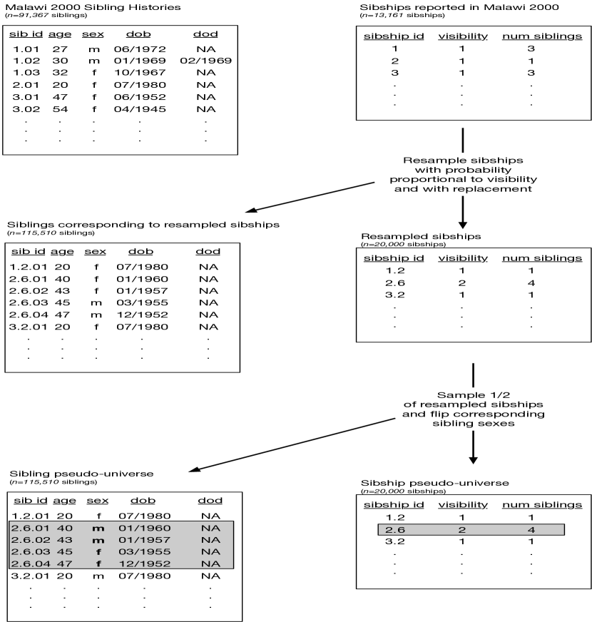
Figure 8: Overview of the method used to construct a pseudo-universe that forms the basis for the simulation study.

The result is a universe of siblings who are assigned to sibships that is approximately representative of the 2000 Malawi sibship population. Figure 9 and Figure 10 show the age-sex distribution and death rates in the simulated universe. From the universe of siblings and sibships, we create a sibship network igraph object. We also create a census dataset, and use it as the basis for calculating true death rates by age and sex.

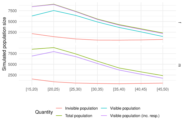
Figure 9: Age-sex distribution of the simulated population.

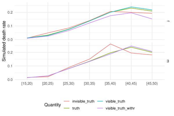
Figure 10: Age- and sex-specific death rates among members of the simulated population.

.J.2 Simulating reporting error and sampling

Having created a pseudo-universe of siblings linked together in sibships, the goal is to use this population as the basis for simulated sibling history surveys under different scenarios. By scenario, we mean a set of aggregate reporting parameters together with a sampling fraction. We now describe how we simulate sibling history surveys under several different scenarios.

Using the sibling universe, we create several population-level reporting networks, one for each combination of aggregate reporting parameters $\tau_{D}=\{0.8,1\}$ and $\tau_{N}=\{0.8,1\}$. We assume there are no false positives throughout (i.e., $\eta_{D}=1$ and $\eta_{N}=1$).

For each population reporting network, we calculate all of the aggregate and individual-level adjustment factors.

For each population reporting network, we simulate $M=1000$ sample surveys for each sampling fraction in $f=\{0.05,0.1,0.15,0.3,0.6\}$.

Finally we calculate the four estimates for each simulated survey: aggregate visibility including/excluding the respondent and individual visibility including/excluding the respondent. Within each scenario, these $M$ estimates are the simulated sampling distribution for the given estimator.

To recap, we generate a pseudo-universe of people linked together in sibships based on the actual sibships reported in the 2000 Malawi DHS survey. From this pseudo-universe, we generate many simulated surveys of different sample sizes, and different assumptions about reporting errors. By calculating death rate estimates using the four estimators for each of these simulated surveys and comparing the estimates to the known underlying truth, we can assess how well the sampling distributions of the four estimators recover true death rates under different reporting conditions and sample sizes.

.J.3 Results

.J.3.1 Confirming the accuracy of the sensitivity framework

First, we examine plots that compare the estimands for the aggregate and individual visibility estimators to the true underlying age-specific visible death rates. By examining the estimands, we remove the complication of sampling and focus on the quantity that each estimator would estimate if the entire frame population were interviewed. These plots will confirm the correctness of our analytical frameworks and provide some intuition about how estimators are affected by reporting errors.

Figure 11 compares the true visible death rates (x axis) to the adjusted and unadjusted aggregate death rate estimands (y axis). Two important features emerge from Figure 11: first, the adjusted estimands all lie on the diagonal $y=x$ line, confirming the correctness of the sensitivity framework for the aggregate estimator (Equation 54). Second, by comparing the unadjusted estimates across the four reporting scenarios, it is clear that the unadjusted estimands for the scenario in which $\tau_{D}=0.8$ and $\tau_{N}=0.8$ (top-left panel) are nearly as accurate as the scenario in which $\tau_{D}=1$ and $\tau_{N}=1$ (bottom-right panel). Intuitively, this suggests that in some cases imperfect reporting may not be very problematic for the aggregate sibling survival estimator, as long as the imperfect reporting is similar for deaths and for exposure; in that case, Figure 11 shows that the reporting errors can cancel out (confirming the intuition from Equation 54).

Figure 12 is analogous to Figure 11, but for the individual visibility estimator.

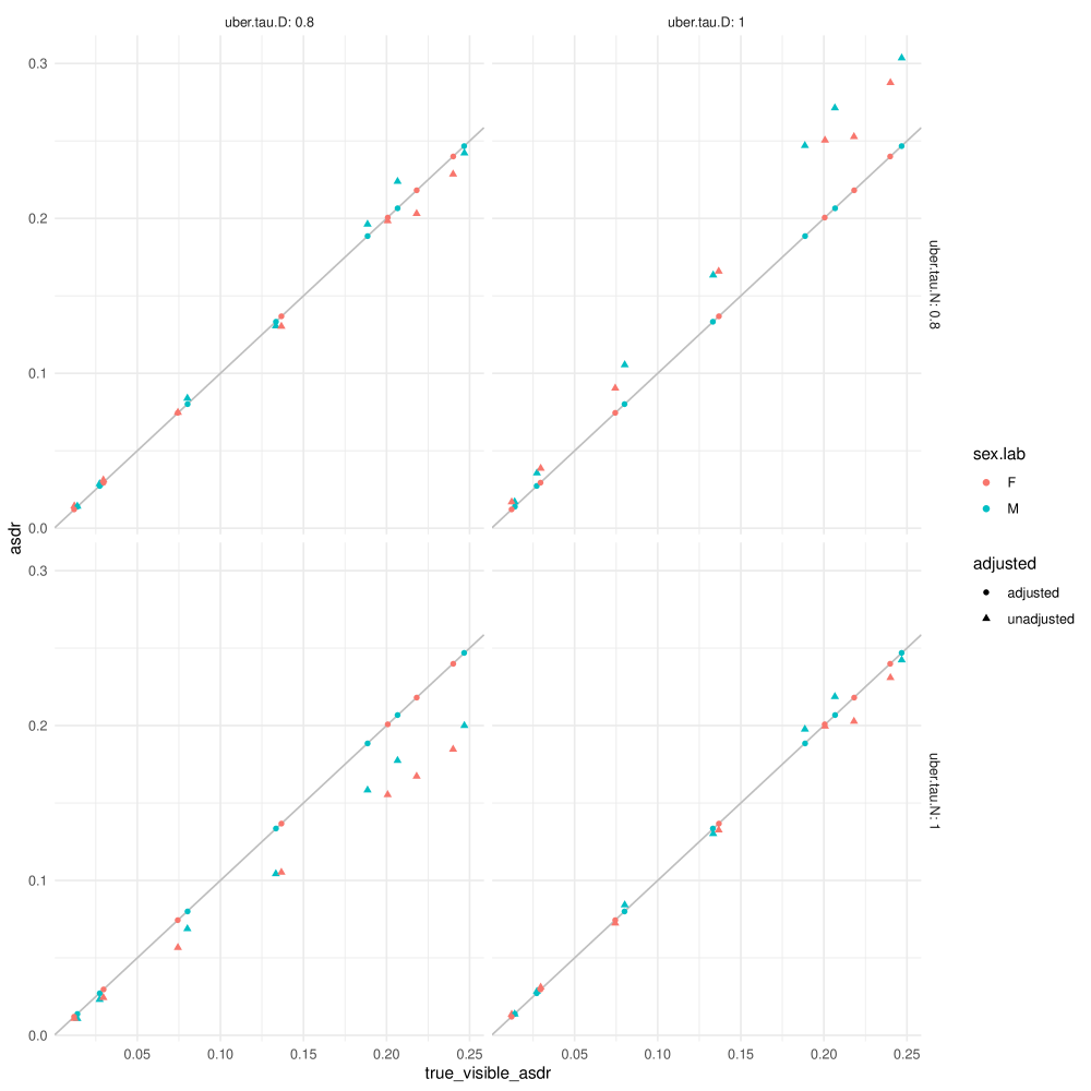
Figure 11: True age-specific death rates (x axis) against adjusted and unadjusted death rate aggregate visibility estimands (y axis). Male death rates are in blue and females are in red. The four panels show four different reporting scenarios. The adjusted estimands all agree with the true underlying death rates, illustrating the correctness of the aggregate sensitivity framework in Equation 54. These results are for the aggregate estimator that does not include the respondent.

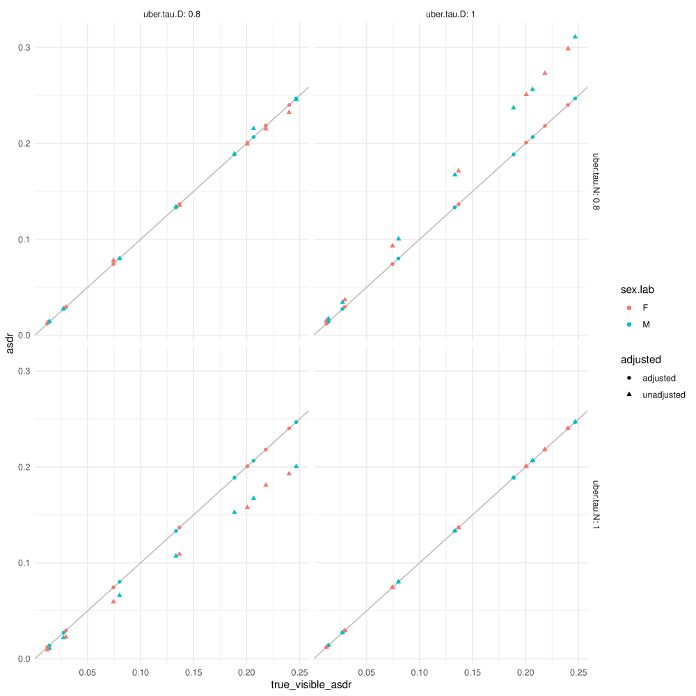
Figure 12: True age-specific death rates (x axis) against adjusted and unadjusted death rate individual visibility estimands (y axis). Male death rates are in blue and females are in red. The four panels show four different reporting scenarios. The adjusted estimands all agree with the true underlying death rates, illustrating the correctness of the individual sensitivity framework in Equation 68 These results are for the individual estimator that does not include the respondent.

.J.3.2 Comparing the estimators

Next, we investigate the performance of the individual and aggregate visibility estimators. In order to evaluate each estimator, we calculated the relative mean square error across the $K=1000$ simulated surveys for each scenario. The relative mean square error of a set of estimates $\widehat{\vec{M}}^{V}$ is

$$\text{rel-MSE}(\widehat{\vec{M}}^{V})=\frac{\sum_{i=1}^{K}(\widehat{M}^{V}_{i}-M^{V})^{2}}{K~{}(M^{V})^{2}}.$$

The relative mean square error can be decomposed into the sum of the squared relative bias:

$$\text{rel-bias}^{2}(\widehat{\vec{M}}^{V})=\left(\frac{\sum_{i=1}^{K}\widehat{M}^{V}_{i}-M^{V}}{K~{}M^{V}}\right)^{2},$$

and the relative variance:

$$\text{rel-var}(\widehat{\vec{M}}^{V})=\frac{\sum_{i=1}^{K}(\widehat{M}^{V}_{i}-\bar{M})^{2}}{(M^{V})^{2}},$$

where $\bar{M}=K^{-1}\sum_{i}\widehat{M}^{V}_{i}$ is the average of the $K$ estimates. Thus, we have

$$\text{rel-MSE}(\widehat{\vec{M}}^{V})=\text{rel-bias}^{2}(\widehat{\vec{M}}^{V})+\text{rel-var}(\widehat{\vec{M}}^{V}).$$

Figure 13 compares the two approaches when the sampling fraction (i.e., the sample size relative to the population size) is 0.05 and reporting is perfect. The figure shows the relative MSE as well as its decomposition into relative squared bias and relative variance. Several observations can be made about Figure 13. First, the magnitude of the relative MSE is comparable for the individual and aggregate visibility estimators, though it is slightly higher using the individual visibility estimator for the oldest age females. Second, the decomposition of the MSE into squared bias and variance reveals that the individual visibility estimator is essentially unbiased – all of its MSE comes from variance. The aggregate visibility estimator, on the other hand, is slightly biased, even in this favorable simulation setup.

Figure 14 compares the two estimators when the sampling fraction is 0.05 but reporting is imperfect; in this scenario, the true positive rate for reports about deaths is 0.8, meaning that some deaths are omitted from reports. Several observations can be made about Figure 14. First, compared to the perfect reporting results shown in Figure 13, the level of relative MSE is higher in Figure 14, presumably due to the reporting errors. Second, again due to the reporting errors, we see now that both the aggregate and individual visibility estimators are biased. Generally, the MSE are again similar between the two approaches, now with some cells producing slightly lower MSE for the individual visibility estimator.

Importantly, both Figure 13 and Figure 14 show the results of scenarios in which there is, by design, no relationship between visibility and mortality. In situations where such a relationship exists, we would expect the individual visibility estimator to tend to perform better than the aggregate visibility estimator, since the individual visibility estimator avoids having to make the assumption that the visibility of deaths is equal to the visibility of exposure.

Future research could extend this simulation analysis to better understand the tradeoffs between these two approaches; our results here (i) confirm that our analytical results are correct; and (ii) illustrate that, in relatively favorable situations, the error from the aggregate and individual visibility estimators is roughly comparable. A deeper understanding of the difference in the two estimators is an important topic for future research.

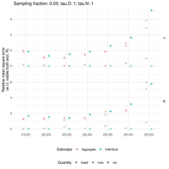
Figure 13: Mean square error, squared bias, and variance for the individual and aggregate visibility estimators when the sampling fraction is 0.05.

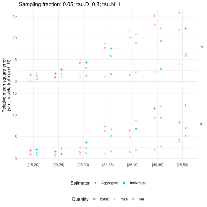
Figure 14: Mean square error, squared bias, and variance for the individual and aggregate visibility estimators when the sampling fraction is 0.05.