$DK$, $DDK$, and $DDDK$ molecules–understanding the nature of the $D_{s0}^{*}(2317)$

Abstract

The $DK$ interaction is strong enough to form a bound state, the $D_{s0}^{*}(2317)$. This in turn begs the question of whether there are bound states composed of several charmed mesons and a kaon. Previous calculations indicate that the three-body $DDK$ system is probably bound, where the quantum numbers are $J^{P}=0^{-}$, $I=\tfrac{1}{2}$, $S=1$ and $C=2$. The minimum quark content of this state is $cc\bar{q}\bar{s}$ with $q=u,d$, which means that, if discovered, it will be an explicitly exotic tetraquark. In the present work. we apply the Gaussian Expansion Method to study the $DDDK$ system and show that it binds as well. The existence of these three and four body states is rather robust with respect to the $DD$ interaction and subleading (chiral) corrections to the $DK$ interaction. If these states exist, it is quite likely that their heavy quark symmetry counterparts exist as well. These three-body $DDK$ and four-body $DDDK$ molecular states could be viewed as counterparts of atomic nuclei, which are clusters of nucleons bound by the residual strong force, or chemical molecules, which are clusters of atoms bound by the residual electromagnetic interaction.

I Introduction

In 2003 the BaBar collaboration discovered the $D_{s0}^{*}(2317)$ Aubert et al. (2003) , a strange-charmed scalar meson, the observation of which was subsequently confirmed by CLEO Besson et al. (2003) and Belle Krokovny et al. (2003). Its mass is about $160\,{\rm MeV}$ below the one predicted for the lightest $c\bar{s}$ scalar state in the naive quark model, which makes it difficult to interpret the $D_{s0}^{*}$ as a conventional $q\bar{q}$ state Bardeen et al. (2003); Nowak et al. (2004); van Beveren and Rupp (2003); Dai et al. (2003); Narison (2005); Szczepaniak (2003); Browder et al. (2004); Barnes et al. (2003); Cheng and Hou (2003); Chen and Li (2004); Dmitrasinovic (2005); Zhang (2019); Terasaki (2003); Maiani et al. (2005).

On the other hand, the $D_{s0}^{*}$ can be easily explained as a dynamically generated state arising from the Weinberg-Tomozawa (WT) $DK$ interaction Kolomeitsev and Lutz (2004); Hofmann and Lutz (2004); Guo et al. (2008, 2006, 2009); Cleven et al. (2011); Martinez Torres et al. (2012); Martínez Torres et al. (2015); Yao et al. (2015); Guo et al. (2015); Albaladejo et al. (2017); Du et al. (2017); Guo et al. (2018a); Albaladejo et al. (2018); Altenbuchinger and Geng (2014); Altenbuchinger et al. (2014); Geng et al. (2010); Wang and Wang (2012); Liu et al. (2009); Guo et al. (2018b, 2019). This has led to the prevailing idea that the $D_{s0}^{*}(2317)$ is a molecular state, a hypothesis which has been further supported by a series of Lattice QCD simulations Liu et al. (2013); Mohler et al. (2013); Lang et al. (2014); Bali et al. (2017). For a recent brief summary of all the experimental, lattice QCD, and theoretical supports for such an assignment, see, e.g., Ref. Guo (2019).

If the $DK$ interaction is strongly attractive, a natural question to ask is what happens when one adds one extra $D$ meson to the system . The answer seems to be that it binds Sanchez Sanchez et al. (2018); Martinez Torres et al. (2019). In Ref. Sanchez Sanchez et al. (2018) it was noticed that the $DD_{s0}^{*}$ system can exchange a kaon near the mass shell, leading to a relatively long-range attractive Yukawa potential that is strong enough to bind. This conclusion is left unchanged if one explicitly considers the composite nature of the $D_{s0}^{*}$, which simply leads to more binding Sanchez Sanchez et al. (2018). A later, more complete calculation in Ref. Martinez Torres et al. (2019) leads to a binding energy of about 90 ${\rm MeV}$ for the $DDK$ three-body system. In the present manuscript we revisit the calculation of the $DDK$ bound state and extend it to the $DDDK$ system by using the Gaussian Expansion Method (GEM), which offers a number of advantages compared to previous studies Sanchez Sanchez et al. (2018); Martinez Torres et al. (2019). First, it allows one to calculate directly the density distribution of the three (four) body system, which then gives a transparent picture for their spacial distributions. Second, it has enough flexibility so that one can study the impact of the existence of a repulsive core. Indeed, the chiral potential kernel up to the next to leading order with the low-energy constants determined by the corresponding lattice QCD data shows that this may indeed be the case Altenbuchinger et al. (2014).

The outcome of the exploration presented in this work is that both the $DDK$ and $DDDK$ systems bind, with binding energies of the order of $65-70$ and $90-100\,{\rm MeV}$ in each case. While the $DDK$ bound state, owing to its $cc\bar{q}\bar{s}$ quark content, might be produced in experiments in the future, the $DDDK$ bound state is more likely to be observed on the lattice instead.

This article is organized as follows. In Sec. II, we explain how we parametrize and determine the two-body $DK$ and $DD$ interactions. In Sec. III, we explain how to construct the three- and four-body $DDK$ and $DDDK$ wave functions and solve the corresponding Schr$\ddot{\rm{o}}$dinger equation using the GEM. In Sec. IV, we present our predictions for the $DDK$ and $DDDK$ bound states and discuss their sensitivity to a series of possible corrections. Finally, we summarize the results of this manuscript in Sect. V.

II The S-wave $DK$ and $DD$ potentials

Table 1: Mass and spin-parity of the $D$, $K$ and $D_{s0}^{*}(2317)$ mesons.

Particles	mass(MeV)	$I(J^{P})$
$D^{\pm}$	1869.65	$\frac{1}{2}(0^{-})$
$D^{0}$	1864.83	$\frac{1}{2}(0^{-})$
$K^{\pm}$	493.677	$\frac{1}{2}(0^{-})$
$K^{0}$	497.611	$\frac{1}{2}(0^{-})$
$D_{s0}^{*}(2317)$	2317.7	$0(0^{+})$

The calculation of the $DDK$ and $DDDK$ bound states depends on the $DK$ and $DD$ two-body interactions. While the $DK$ interaction can be well constrained directly from the assumption that the $D_{s0}^{*}(2317)$ is a $DK$ bound state, and indirectly from chiral perturbation theory, the $DD$ interaction is far from being well determined and we will have to resort to phenomenological models instead. In this section we will explain the type of potentials we will use to model these two-body interactions.

II.1 The $DK$ interaction

The most important contribution to the $DK$ interaction is the WT term between a $D$ meson and a kaon . In the non-relativistic limit we can write this interaction as a standard quantum mechanical potential,

$$V_{DK}(\vec{q})=-\frac{C_{W}(I)}{2f_{\pi}^{2}}$$ (1)

where the pion decay constant $f_{\pi}\approx 130$ MeV and $C_{W}(I)$ represents the strength of the WT interaction, which is

$$C_{W}(0)=2\quad\mbox{and}\quad C_{W}(1)=0\,,$$ (2)

depending on whether we are considering the isospin $I=0$ or $I=1$ configuration of the $DK$ system. The Fourier-transform of the previous potential in coordinate space is

$$V_{DK}(\vec{r})=-\frac{C_{W}(I)}{2f_{\pi}^{2}}\,\delta^{(3)}(\vec{r})\,,$$ (3)

which has to be regularized before being used within the Schrödinger equation. A possible choice is to use a local Gaussian regulator of the type

$$V_{DK}({r};R_{c})=-\frac{C_{W}(I)}{2f_{\pi}^{2}}\,\frac{e^{-(r/R_{c})^{2}}}{\pi^{3/2}R_{c}^{3}}\,,$$ (4)

where $R_{c}$ is the cutoff we use to smear the delta function. For sensible choices of the cutoff, this potential reproduces the $D_{s0}^{*}$ pole. Nowadays we consider the WT interaction as the leading order (LO) term in the chiral expansion of the $DK$ potential Geng et al. (2010); Altenbuchinger et al. (2014). In this regard it is interesting to notice that even though LO chiral perturbation theory (ChPT) indeed indicates that the $I=0$ $DK$ interaction in S-wave is attractive, it happens that the next-to-leading order (NLO) correction is weakly repulsive, see e.g. Ref. Altenbuchinger et al. (2014). This motivates the inclusion of a short-range repulsive core in the $DK$ interaction, as we will explain in the next paragraph.

For the present purposes a more practical approach will be to consider the $DK$ interaction in a contact-range effective field theory, in which at LO we have the (already regularized) potential

$$V_{DK}({r};R_{c})=C(R_{C})\,\frac{e^{-(r/R_{c})^{2}}}{\pi^{3/2}R_{c}^{3}}\,,$$ (5)

with $R_{c}$ the cutoff and where the $C(R_{c})$ is now a running coupling constant. The differences with a unitarized WT term are (i) that we let the cutoff $R_{c}$ to float and (ii) that we consider the strength of the interaction to run with the cutoff. In this way by varying the cutoff within a sensible range, for which we choose $R_{c}=1-3\,{\rm fm}$ in this work, we can estimate the uncertainty in the calculations coming from subleading corrections. We advance that the cutoff variation will be tiny. Besides the variation of the cutoff, we will consider a second method to assess the error in our calculations. Inspired by the fact that ChPT predicts a repulsive core in the $DK$ interaction at NLO (as previously mentioned), we can explicitly include this core in the potential

$$V_{DK}(\vec{r};R_{c})=C_{S}\,\frac{e^{-(r/R_{S})^{2}}}{\pi^{3/2}R_{S}^{3}}+C(R_{C})\,\frac{e^{-(r/R_{c})^{2}}}{\pi^{3/2}R_{c}^{3}}=C^{\prime}_{S}e^{-(r/R_{S})^{2}}+C^{\prime}_{L}e^{-(r/R_{c})^{2}}\,,$$ (6)

where $C_{S}$ is a coupling constant that we set as to provide a repulsive core, i.e. we take $C^{\prime}_{S}>|C^{\prime}_{L}|$, and $R_{S}$ is a second cutoff which fulfills the condition $R_{S}<R_{c}$. For concreteness we take $R_{S}=0.5\,{\rm fm}$.

II.2 The DD interaction

The $DD$ interaction is not known experimentally, but there are phenomenological models for it. Here we will consider the one boson exchange (OBE) potential, which provides a very simple and intuitive description of the hadron-hadron interactions. The first qualitatively successful description of the two-nucleon potential used the OBE model Machleidt et al. (1987); Machleidt (1989), and the same is true for the first speculations about the existence of heavy hadron molecules Voloshin and Okun (1976). The particular version of the OBE model that we will use is the one in Ref. Liu et al. (2019), developed for the description of heavy meson-meson and heavy meson-antimeson systems.

In the particular case of the $DD$ two-body system, the OBE potential involves the exchange of the $\sigma$, $\rho$ and $\omega$ mesons:

$$V_{DD}(r;\Lambda)=V_{\rho}(r;\Lambda)+V_{\omega}(r;\Lambda)+V_{\sigma}(r;\Lambda)$$ (7)

where the contribution of each light meson is regularized by means of a form factor and $\Lambda$ is a cutoff. The particular contribution of each meson can be written as Liu et al. (2019)

$$V_{\sigma}(r;\Lambda) = -g_{\sigma}^{2}\,m_{\sigma}\,W_{C}(m_{\sigma}r,\frac{\Lambda}{m_{\sigma}})\,,$$ (8)

$$V_{\rho}(r;\Lambda) = +\vec{\tau}_{1}\cdot\vec{\tau}_{2}\,g_{\rho}^{2}\,m_{\rho}\,W_{C}(m_{\rho}r,\frac{\Lambda}{m_{\rho}})\,,$$ (9)

$$V_{\omega}(r;\Lambda) = +g_{\omega}^{2}\,m_{\omega}\,W_{C}(m_{\omega}r,\frac{\Lambda}{m_{\omega}})\,,$$ (10)

where

$$W_{C}(x,\lambda)=\frac{e^{-x}}{4\pi x}-\lambda\,\frac{e^{-\lambda x}}{4\pi\lambda x}-\frac{(\lambda^{2}-1)}{2\lambda}\,\frac{e^{-\lambda x}}{4\pi}.$$ (11)

The masses of the bosons we use are $m_{\rho}=0.770$ GeV, $m_{\omega}=0.780$ GeV, $m_{\sigma}=0.6$ GeV, and the couplings are $g_{\rho}=g_{\omega}=2.6$, $g_{\sigma}=3.4$. The cutoff is set by reproducing the $X(3872)$ pole, yielding $\Lambda=1.01^{+0.19}_{-0.10}\,{\rm GeV}$ Liu et al. (2019). Here for the sake of simplicity we will set the cutoff to $\Lambda=1.0\,{\rm GeV}$, where we note that the cutoff dependence is weak.

III Gaussian Expansion Method to solve the 3-body $DDK$ and 4-body $DDDK$ systems

In this section we briefly explain the Gaussian Expansion Method (GEM) Kamimura (1988); Hiyama et al. (2003) as applied to the $DDK$ and $DDDK$ systems. In the past the GEM has been successfully applied in hypernuclear as well as heavy-hadron systems. The focus of the manuscript is on the one hand to confirm the previous theoretical studies about the existence of a $DDK$ bound state and to explore whether there are also bound $DDDK$ tetramers. Regarding the $DDK$ system, it was investigated in Ref. Sanchez Sanchez et al. (2018) first as a $DD_{s0}^{*}$ two-body system, a description which is valid provided that the size of the $DDK$ trimer is larger than its components (in particular the $D_{s0}^{*}$ meson), and second as a genuine three-body system by solving the Faddeev equations. In each case the bound state is at about $(50-60)\,{\rm MeV}$ and $(60-100)\,{\rm MeV}$ below the $DDK$ threshold, respectively. Later a more complete study appeared in Ref. Martinez Torres et al. (2019), which uses the method developed by the Valencia group Martinez Torres et al. (2008a); Khemchandani et al. (2008); Martinez Torres et al. (2008b, 2009a, 2009b, 2009c); Martinez Torres and Jido (2010); Martinez Torres et al. (2011a, b) to solve the Faddeev equation Faddeev (1961) for the $DDK$ system, predicting a bound state at about $90\,{\rm MeV}$ below the $DDK$ threshold.

III.1 Three-body $DDK$ system

The Schrödinger equation of the $DDK$ 3-body system is

$$H\Psi_{JM}^{total}=E\Psi_{JM}^{total},$$ (12)

with the corresponding Hamiltonian

$$\hat{H}=\sum_{i=1}^{3}\frac{p_{i}^{2}}{2m_{i}}-T_{c.m.}+\sum_{1=i<j}^{3}V(r_{ij}),$$ (13)

where $T_{c.m.}$ is the kinetic energy of the center of mass and $V(r_{ij})$ is the potential between the $i$-th and the $j$-th particle pair. The three Jacobi coordinates for the $DDK$ system are shown in Fig. 1.

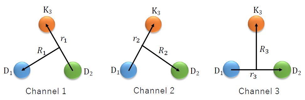
Figure 1: The three permutations of the Jacobi coordinates for the $DDK$ system

The total wave function is a sum of the amplitudes of the three possible rearrangement of the Jacobi coordinates, i.e. of the channels ($c=1-3$) shown in Fig. 1

$$\Psi_{JM}^{total}=\sum_{c,\alpha}C_{c,\alpha}\,\Psi_{JM,\alpha}^{c}(\mathbf{r}_{c},\mathbf{R}_{c})\,,$$ (14)

where $\alpha=\{nl,NL,\Lambda,tT\}$ and $C_{c,\alpha}$ are the expansion coefficients. Here $l$ and $L$ are the orbital angular momenta for the coordinates $r$ and $R$, $t$ is the isospin of the two-body subsystem in each channel, $\Lambda$ and $T$ are the total orbital angular momentum and isospin, $n$ and $N$ are the numbers of Gaussian basis function corresponding to coordinates $r$ and $R$, respectively. For the $DD$ and $DK$ two-body potentials we refer to Sect. II. The eigen energy $E$ and coefficients are determined by the Rayleigh-Ritz variational principle. Considering that the two $D$ mesons are identical, the total wave function should be symmetric with respect to the exchange of the two $D$ mesons, which requires that

$$P_{12}\Psi_{JM}^{total}=\Psi_{JM}^{total},$$ (15)

and $P_{12}$ is the exchange operator of particles 1 and 2. The wave function of each channel has the following form

$$\Psi_{JM,\alpha}^{c}(\mathbf{r}_{c},\mathbf{R}_{c})=H_{T,t}^{c}\otimes[\Phi_{lL,\Lambda}^{c}]_{JM}\,,$$ (16)

where $H_{T,t}^{c}$ is the isospin wave function, and $\Phi_{lL,\Lambda}^{c}$ the spacial wave function. The total isospin wave function reads as

$$\begin{split}H_{T,t}^{c=1}&=[[\eta_{\frac{1}{2}}(D_{2})\eta_{\frac{1}{2}}(K_{3})]_{t_{1}}\eta_{\frac{1}{2}}(D_{1})]_{\frac{1}{2}}\,,\\ H_{T,t}^{c=2}&=[[\eta_{\frac{1}{2}}(D_{1})\eta_{\frac{1}{2}}(K_{3})]_{t_{2}}\eta_{\frac{1}{2}}(D_{2})]_{\frac{1}{2}}\,,\\ H_{T,t}^{c=3}&=[[\eta_{\frac{1}{2}}(D_{1})\eta_{\frac{1}{2}}(D_{2})]_{t_{3}}\eta_{\frac{1}{2}}(K_{3})]_{\frac{1}{2}}\,,\end{split}$$ (17)

where $\eta$ is the isospin wave function of each particle. The spacial wave function $\Phi_{lL,\Lambda}^{c}$ is given in terms of the Gaussian basis functions

$$\Phi_{lL,\Lambda}^{c}(\mathbf{r}_{c},\mathbf{R}_{c})=[\phi_{n_{c}l_{c}}^{G}(\mathbf{r}_{c})\psi_{N_{c}L_{c}}^{G}(\mathbf{R}_{c})]_{\Lambda},$$ (18)

$$\phi_{nlm}^{G}(\mathbf{r}_{c})=N_{nl}r_{c}^{l}e^{-\nu_{n}r_{c}^{2}}Y_{lm}({\hat{r}}_{c})\,,$$ (19)

$$\psi_{NLM}^{G}(\mathbf{R}_{c})=N_{NL}R_{c}^{L}e^{-\lambda_{n}R_{c}^{2}}Y_{LM}({\hat{R}}_{c})\,.$$ (20)

Here $N_{nl}(N_{NL})$ are the normalization constants of the Gaussian basis and the range parameters $\nu_{n}$ and $\lambda_{n}$ are given by

$$\begin{split}\nu_{n}&=1/r_{n}^{2},\qquad r_{n}=r_{min}a^{n-1}\quad(n=1,n_{max})\,,\\ \lambda_{N}&=1/R_{N}^{2},\quad R_{N}=R_{min}A^{N-1}\quad(N=1,N_{max})\,,\end{split}$$ (21)

in which $\{n_{max},r_{min},a$ or $r_{max}\}$ and $\{N_{max},R_{min},A$ or $R_{max}\}$ are Gaussian basis parameters. After the basis expansion, the Schrödinger equation of this system is transformed into a generalized matrix eigenvalue problem:

$$[T_{\alpha\alpha^{\prime}}^{ab}+V_{{\alpha\alpha^{\prime}}}^{ab}-EN_{\alpha\alpha^{\prime}}^{ab}]\,C_{b,\alpha^{\prime}}=0\,.$$ (22)

Here, $T_{\alpha\alpha^{\prime}}^{ab}$ is the kinetic matrix element, $V_{\alpha\alpha^{\prime}}^{ab}$ is the potential matrix element and $N_{\alpha\alpha^{\prime}}^{ab}$ is the normalization matrix element.

The quantum numbers of all the allowed configurations are determined by angular momentum conservation, isospin conservation, parity conservation, and Bose-Einstein statistics. Given that we only consider $S$-wave interactions, and only the $DK$ interaction in $I=0$ is dominant, we obtain the allowed configurations shown in Table 2. The $DDK$ system that we are interested in has isospin 1/2 and spin parity $0^{-}$.

Table 2: Quantum numbers of different Jacobi coordinate channels $(c=1-3)$ of the $DDK$ $I(J^{P})=\frac{1}{2}(0^{-})$ state. Note that channel 1 and channel 2 are the same.

c	$l$	$L$	$\Lambda$	$t$	$T$	$J$	$P$
1(2)	0	0	0	0	$\frac{1}{2}$	0	$-$
1(2)	0	0	0	1	$\frac{1}{2}$	0	$-$
3	0	0	0	1	$\frac{1}{2}$	0	$-$

III.2 Four-body $DDDK$ system

A generic four-body system has 18 Jacobi coordinates. In the $DDDK$ system, owing to the fact that there are three identical $D$ mesons, the possible configurations of the Jacobi coordinates reduce to three K-type channels and one H-type channel, see Fig.[2]. There are 4 identical Jacobi coordinates for each K-type channel and 6 identical Jacobi coordinates for the H-type channel.

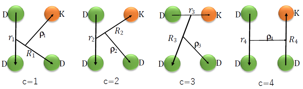
Figure 2: Jacobi coordinates for the rearrangement channels ($c=1-4$) of the $DDDK$ system. The three $D$ mesons are to be symmetrized.

The total wave function of this $DDDK$ system is

$$\Psi_{I(J^{P})}^{total}=\sum_{c,\alpha}A_{c,\alpha}\Psi_{\alpha}^{c}(\bm{r}_{c},\bm{R}_{c},\bm{\rho}_{c}),\qquad c=1-18\,,$$ (23)

and the wave function in each Jacobi channel reads

$$\Psi_{\alpha}^{c}(\bm{r}_{c},\bm{R}_{c},\bm{\rho}_{c})=H_{t,T,I}^{c}\otimes\Phi_{lL\lambda,\sigma\Lambda}^{c,JP}\,.$$ (24)

Here $t,T,I$ are the isospin of the coordinates $r,R$ and $\rho$ in each channel; $l,L$ and $\lambda$ are the orbital angular momenta for the coordinates $r,R$ and $\rho$, while $\sigma$ is the coupling of $l$ and $L$, $\Lambda$ is the coupling of $\sigma$ and $\lambda$, and $J,P$ is the total angular momentum and parity. The Gaussian basis and parameters are in the same form as those in the 3-body system, which are

$$\Phi_{lL\lambda,\sigma\Lambda}^{c}=[\phi_{n_{c}l_{c}}^{G}(\bm{r}_{c})\psi_{N_{c}L_{c}}^{G}(\bm{R}_{c})]_{\sigma_{c}}\varphi_{\nu_{c}\lambda_{c}}^{G}(\bm{\rho}_{c})]_{\Lambda}\,,$$ (25)

$$\phi_{nlm}^{G}(\bm{r}_{c})=N_{nl}r_{c}^{l}e^{-\nu_{n}r_{c}^{2}}Y_{lm}({\hat{r}}_{c})\,,$$ (26)

$$\psi_{NLM}^{G}(\bm{R}_{c})=N_{NL}R_{c}^{L}e^{-\lambda_{N}R_{c}^{2}}Y_{LM}({\hat{R}}_{c})\,,$$ (27)

$$\varphi_{\nu\lambda\mu}^{G}(\bm{\rho}_{c})=N_{\nu\lambda}\rho_{c}^{\lambda}e^{-\omega_{\nu}\rho_{c}^{2}}Y_{\lambda\mu}({\hat{\rho}}_{c})\,.$$ (28)

Here $N_{nl}(N_{NL})$ are the normalization constants of the Gaussian basis and the range parameters $\nu_{n}$, $\lambda_{n}$ and $\omega_{\nu}$ are given by

$$\begin{split}\nu_{n}&=1/r_{n}^{2},\qquad r_{n}=r_{min}a^{n-1}\quad(n=1,n_{max})\,,\\ \lambda_{N}&=1/R_{N}^{2},\quad R_{N}=R_{min}A^{N-1}\quad(N=1,N_{max})\,,\\ \omega_{\nu}&=1/\rho_{\nu}^{2},\qquad\rho_{\nu}=\rho_{min}\alpha^{\nu-1}\quad(\nu=1,\nu_{max})\,.\\ \end{split}$$ (29)

Since we are considering only $S$-wave interactions, we have $J=l=L_{\lambda}=\sigma=\Lambda=0$, and the parity is $+$. The procedure to determine the allowed configurations for the $DDDK$ system is the same as the $DDK$ case. The 4-body $DDDK$ configurations are shown in Table.3.

Table 3: Quantum numbers of different Jacobi coordinate channels $(c=1-4)$ of the $DDDK$ $I(J^{P})=1(0^{+})$ state. The identical channels have the same configuration. The number in the brackets denotes the alternative value.

c	$l$	$L$	$\lambda$	$\sigma$	$L$	$t$	$T$	$I$	$J$	$P$
1	0	0	0	0	0	1	$\frac{1}{2}(\frac{3}{2})$	1	0	$+$
2	0	0	0	0	0	1	$\frac{1}{2}(\frac{3}{2})$	1	0	$+$
3	0	0	0	0	0	0(1)	$\frac{1}{2}(\frac{3}{2})$	1	0	$+$
4	0	0	0	0	0	1	0(1)	1	0	+

IV Predictions

In this section we discuss the predictions we make for the $DDK$ and $DDDK$ bound states. With the two-body inputs of Sect. II and the three(four)-body configurations detailed in Sect. III, we can predict the existence of $DDK$ and $DDDK$ bound states. The outcome is that the $DDK$ trimer will bind by about $70\,{\rm MeV}$ and the $DDDK$ tetramer by about $100\,{\rm MeV}$, with variations of a few ${\rm MeV}$ at most, stemming from the uncertainties in the $DK$ and $DD$ potentials.

IV.1 Solving the $DDK$ and $DDDK$ systems

The two basic input blocks for the calculation of the $DDK$ and $DDDK$ systems are the $DK$ and $DD$ interactions, of which the $DK$ one is the most important factor when it comes to binding. The $DK$ potential contains the running coupling $C(R_{c})$ and the cutoff $R_{c}$, where $R_{c}=(1-3)\,{\rm fm}$ and $C(R_{c})$ is determined from the condition of reproducing the well-known $D_{s0}^{*}(2317)$ as a $DK$ bound state with a binding energy of $45\,{\rm MeV}$. In addition there are two additional parameters, the coupling $C_{S}$ and the short-range radius $R_{s}=0.5\,{\rm fm}$, which are used to estimate the uncertainties in the $DK$ potential. We study three combinations of $R_{S}$ and $R_{c}$, which can be consulted in Table 4, where we also list the values of the couplings $C_{R}$ and $C(R_{c})$ and the binding energies of the $DDK$ and $DDDK$ systems. The different potentials investigated are shown in Fig. 3 and the probability density distributions of the $DK$ pair corresponding to the potentials are shown in Fig. 4.

Table 4: Binding energies (in units of MeV) of $DDK$ and $DDDK$ systems with and without the $DD$ interaction for different combinations of $R_{S}$, $R_{c}$, $C^{\prime}_{S}$, and $C^{\prime}_{L}$. The couplings are in units of MeV.

$C^{\prime}_{S}$	$C^{\prime}_{L}$	$E_{2}$	$E_{3}$(only $V_{DK})$	$E_{3}(V_{DK}+V_{DD})$	$E_{4}($only $V_{DK})$	$E_{4}(V_{DK}+V_{DD})$
		$R_{S}=0.5$ fm		$R_{c}=1$ fm
0	$-320.1$	$-45.0$	$-65.8$	$-71.2$	$-89.4$	$-106.8$
$500$	$-455.4$	$-45.0$	$-65.8$	$-70.4$	$-89.2$	$-103.5$
$1000$	$-562.6$	$-45.0$	$-65.7$	$-69.7$	$-88.8$	$-101.4$
$3000$	$-838.7$	$-45.0$	$-65.0$	$-68.4$	$-87.0$	$-97.3$
		$R_{S}=0.5$ fm		$R_{c}=2$ fm
0	$-149.1$	$-45.0$	$-66.0$	$-68.8,-45.1$	$-88.7,-66.3$	$-97.6,-70.7$
$500$	$-178.4$	$-45.0$	$-65.9$	$-68.2,-45.5$	$-88.5,-66.7$	$-95.5,-70.9$
$1000$	$-195.0$	$-45.0$	$-65.8,-45.2$	$-67.9,-45.8$	$-88.2,-66.9$	$-94.5,-71.2$
$3000$	$-225.9$	$-45.0$	$-65.3,-45.6$	$-67.2,-46.6$	$-87.0,-67.0$	$-92.6,-71.7$
		$R_{S}=0.5$ fm		$R_{c}=3$ fm
0	$-107.0$	$-45.0$	$-66.2,-47.3$	$-68.0,-48.3$	$-88.8,-70.2$	$-94.4,-74.3$
$500$	$-119.4$	$-45.0$	$-66.2,-48.2$	$-67.7,-49.3$	$-88.7,-71.0$	$-93.2,-74.8$
$1000$	$-125.6$	$-45.0$	$-66.1,-48.7$	$-67.5,-49.8$	$-88.4,-71.3$	$-92.5,-75.2$
$3000$	$-136.2$	$-45.0$	$-65.8,-49.4$	$-67.1,-50.7$	$-87.6,-71.7$	$-91.4,-75.7$

Table 5: Root mean square (RMS) radius (in units of fm) of $DK$ and $DDK$ systems, the expectation values (in units of MeV) of the kinetic term, $DK$ and $DD$ interactions with various parameters $R_{S}$. $R_{c}$, $C^{\prime}_{S}$, and $C^{\prime}_{L}$. The couplings are in units of MeV.

$C^{\prime}_{S}$	$C^{\prime}_{L}$	$r_{2}(DK)$	$r_{3}(DK)$	$r_{3}(DD)$	$<T>$	$<V_{DK}>$	$<V_{DD}>$
		$R_{S}=0.5$ fm		$R_{c}=1$ fm
0	$-320.1$	1.28	$1.32$	1.36	$124.37$	$-189.61$	$-5.98$
$500$	$-455.4$	1.39	$1.44$	1.47	$99.51$	$-164.83$	$-5.03$
$1000$	$-562.6$	1.46	$1.53$	1.54	$91.43$	$-156.67$	$-4.51$
$3000$	$-838.7$	1.61	$1.69$	1.68	$93.24$	$-157.80$	$-3.82$
		$R_{S}=0.5$ fm		$R_{c}=2$ fm
0	$-149.1$	1.74	$1.80$	1.80	$60.20$	$-125.74$	$-3.23$
$500$	$-178.4$	1.91	$1.98$	1.96	$51.00$	$-116.59$	$-2.64$
$1000$	$-195.0$	1.99	$2.07$	2.04	$50.63$	$-116.12$	$-2.43$
$3000$	$-225.9$	2.13	$2.22$	2.15	$53.61$	$-118.59$	$-2.24$
		$R_{S}=0.5$ fm		$R_{c}=3$ fm
0	$-107.0$	$2.13$	$2.19$	2.17	$39.49$	$-105.35$	$-2.13$
$500$	$-119.4$	$2.31$	$2.38$	2.34	$34.80$	$-100.73$	$-1.77$
$1000$	$-125.6$	$2.37$	$2.47$	2.42	$34.90$	$-100.77$	$-1.65$
$3000$	$-136.2$	$2.53$	$2.61$	2.53	$36.66$	$-102.24$	$-1.54$

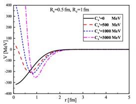
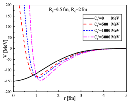
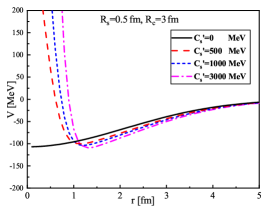
Figure 3: Isospin $t=0$ $DK$ potential as a function of the distance between $D$ and $K$ for different $R_{S}$, $R_{c}$, and $C^{\prime}_{S}$. The coupling $C^{\prime}_{L}$ in each case is determined by reproducing the $D_{s0}^{*}$.

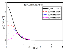
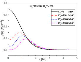
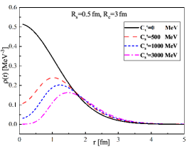
Figure 4: Density profile of the $DK$ molecule corresponding to the potentials of Fig. 3.

A few comments about the results of Table 4 are in order. The first thing we notice is that the impact of the $DD$ interaction is mild. It makes the $DDK$ and $DDDK$ systems more bound, but only by a few ${\rm MeV}$. This is a bit relieving as the $DD$ interaction is not well known. The second interesting observation is that the existence of the $DDK$ and $DDDK$ bound states is rather robust with respect to the likely existence of a short-range repulsive core. In other words, the existence of the $DDK$ and $DDDK$ bound states is almost guaranteed as long as the $D_{s0}^{*}$ is dominantly a $DK$ bound state (we will later check that this will still be the case even if the $D_{s0}^{*}$ is a compact ${\bar{c}}s$ state). The third observation is that as the range of the attraction becomes larger, two bound state solutions appear instead of one, with the deepest bound one becoming slightly shallower.

In Table 5 we show the root mean square (RMS) radius of the $DK$ and $DDK$ systems as well as the expectation values of the kinetic and potential terms. The RMS radius of the $D_{s0}^{*}$, which ranges from $1.2$ to $2.6$ fm, increases with the cutoff $R_{c}$ and with the coupling $C_{S}$ of the short-range repulsive core. In the $DDK$ system, the RMS radius of the $DK$ pair is slightly larger than its counterpart in the $D_{s0}^{*}$. The RMS radius of the $DD$ system also increases if we increase the cutoff $R_{c}$ or the coupling $C_{S}$. We notice that the geometry of the $DDK$ system is more or less of a proper triangle, which agrees qualitatively with the findings of Ref. Martinez Torres et al. (2019). From the last two columns of Table 5, it is clear that the $DD$ interaction is weakly attractive, accounting for only a few ${\rm MeV}$ of the total potential energy.

IV.2 Solving the $DDDK$ system as an equivalent $DDD_{s0}^{*}$ system

If the separation of the $DK$ pair within the $DDK$ trimer and $DDDK$ tetramer is comparable to or larger than the expected size of the $D_{s0}^{*}$, in a first approximation it will be possible to treat the $D_{s0}^{*}$ as a point-like particle, with its compound structure providing subleading corrections to this point-like approximation. From Table 5 we can see that the RMS of the $DK$ subsystem in the $DDK$ and $DDDK$ systems is similar to that of the $D_{s0}^{*}$ as a $DK$ molecule. In this regard we notice that in Ref. Sanchez Sanchez et al. (2018) the $D_{s0}^{*}$ is approximated as point-like, where the interaction between the $D$ and $D_{s0}^{*}$ is mediated by one kaon exchange and is strong enough to form a bound state. This $DD_{s0}^{*}$ molecule is predicted to be $50-60\,{\rm MeV}$ below the $DDK$ threshold, to be compared with $65\,{\rm MeV}$ when we consider it as a genuine $DDK$ three-body state and ignore the $DD$ interaction (see Table 4). This indicates that the predictions of the point-like approximation are reasonably good (for such a simple approximation) and that the compound structure of the $D_{s0}^{*}$ provides additional attraction. In the following lines we will extend the ideas of Ref. Sanchez Sanchez et al. (2018) to the $DDDK$ tetramer, i.e. we will treat it as a three-body $DDD_{s0}^{*}$ system where the $D_{s0}^{*}$ is assumed to be a compact meson. To do this, we first reproduce the two-body calculation of Ref. Sanchez Sanchez et al. (2018), but in coordinate space, and then study the three-body $DDD_{s0}^{*}$ system using the GEM.

The interaction of $DD_{s0}^{*}$ is attractive and reads as

$$V_{OKE}(\vec{q})=-h^{2}\frac{\omega_{K}^{2}}{f_{\pi}^{2}}\frac{1}{\mu_{K}^{2}+\vec{q}^{2}},$$ (30)

where $\omega_{K}=m_{D_{s0}^{*}}-m_{D}$ and the effective kaon mass $\mu_{K}=\sqrt{m_{K}^{2}-\omega_{K}^{2}}$. As in Ref. Sanchez Sanchez et al. (2018), we take $h=0.7$ and $f_{\pi}=130$ MeV. We regularize the potential by multiplying it with a dipole form factor of the type:

$$F_{D}(q^{2})=\frac{(\Lambda^{2}-m_{K}^{2})^{2}}{(\Lambda^{2}-q^{2})^{2}}\,.$$ (31)

After the inclusion of this form factor, the $DD_{s0}^{*}$ potential in coordinate space reads

$$V_{DD_{so}^{*}}(r)=-h^{2}\frac{\omega_{K}^{2}}{f_{\pi}^{2}}\left(\frac{e^{-\mu_{K}r}}{4\pi r}-\frac{e^{-\Lambda^{\prime}r}}{4\pi r}-\frac{(\Lambda^{\prime 2}-\mu_{K}^{2})e^{-\Lambda^{\prime}r}}{8\pi\Lambda^{\prime}}\right)\,,$$ (32)

where we define $\Lambda^{\prime}$ as

$$\Lambda^{\prime 2}=\Lambda^{2}-q_{0}^{2}=\Lambda^{2}-\omega_{K}^{2}\,.$$ (33)

Using the above $DD_{s0}^{*}$ potential and the $DD$ potential provided by the OBE model, we can check whether the three-body $DDD_{s0}^{*}$ system binds. The binding energies we obtain with different cutoffs are tabulated in Table 6.

Table 6: Binding energies (in units of MeV) of $DD_{s0}^{*}$ and ${DDD_{s0}^{*}}$ systems with different cutoff $\Lambda^{\prime}$ (in units of GeV).

$\Lambda^{\prime}$	$B_{DD_{s0}^{*}}$	$B_{DDD_{s0}^{*}}$(only $V_{DD_{s0}^{*}}$)	$B_{DDD_{s0}^{*}}$($V_{DD}+V_{DD_{s0}^{*}}$)
0.8	$-5.1$	$-11.5$	$-13.9$
1.0	$-8.5$	$-18.9$	$-22.5$
1.2	$-11.7$	$-25.8$	$-30.3$
1.4	$-14.5$	$-31.9$	$-37.2$
1.6	$-17.0$	$-37.2$	$-43.3$

With the effective cutoff $\Lambda^{\prime}$ ranging from $0.8-1.6$ GeV, the results of Table.6 indicate that the $DDD_{s0}^{*}$ bound state is located about $(65-90)\,{\rm MeV}$ below the $DDDK$ threshold. This is to be compared with $100\,{\rm MeV}$ for the full four-body calculation, see Table.4 for details. That is, as happened with the $DD_{s0}^{*}$ / $DDK$ system, the approximation that the $D_{s0}^{*}$ is a compact state results in underbinding for the $DDD_{s0}^{*}$ / $DDDK$ system, but not much.

V Summary

In this manuscript we argued that the $DK$ interaction is attractive enough as to generate $DK$, $DDK$ and $DDDK$ bound states. For this we began by assuming that the $D_{s0}^{*}(2317)$ is a $DK$ molecule, which determines in turn the $DK$ interaction. Then, by means of the Gaussian Expansion Method Kamimura (1988); Hiyama et al. (2003) (a method for few-body calculations), we have addressed the question of whether one can build up multi-component molecular states, similar to the formation of atomic nuclei from clusters of nucleons bound by the nucleon-nucleon interaction. The answer is yes. We find a bound $DDK$ trimer and a $DDDK$ tetramer. The prediction of this trimer confirms the previous calculations of Refs. Sanchez Sanchez et al. (2018); Martinez Torres et al. (2019), while the prediction of the tetramer is novel to the present work.

We have checked the robustness of these predictions against a series of uncertainties. While the $DK$ interaction is well constrained by the existence of the $D_{s0}^{*}(2317)$ and chiral perturbation theory, the $DD$ interaction is considerably less well-known. Yet it also enters the calculations. We chose to describe the $DD$ potential in terms of the OBE model, in which the $DD$ interaction turns out to be mildly attractive and has a minor impact on the binding energy of the trimer and tetramer states. The $DK$ potential, though well-known, is still subject to subleading corrections, which we take into account by varying the exact form of this potential. As expected from the fact that we are dealing with subleading corrections, the predictions are almost left unchanged by these variations.

In addition, we have studied a rather unlikely scenario that the $D_{s0}^{*}(2317)$ is dominanty a genuine $c\bar{s}$ state. Nonetheless, even in such a case, we still predict $DD_{s0}^{*}$ and $DDD_{s0}^{*}$ bound states with the same quantum numbers as the $DDK$ trimer and $DDDK$ tetramer, but this time located at approximately $(50-62)$ and $(60-90)\,{\rm MeV}$ below the $DDK$ and $DDDK$ thresholds (instead of $70$ and $100\,{\rm MeV}$ when the $D_{s0}^{*}$ is a molecular meson). The binding mechanism is the long-range one-kaon-exchange potential in the $DD_{s0}^{*}$ system: owing to the mass difference between the $D$ and $D_{s0}^{*}$ mesons, the kaon is exchanged near the mass shell, leading to an enhancement in the range of the potential Sanchez Sanchez et al. (2018).

Although the existence of the $DDK$ and $DDDK$ bound states seems to be quite robust, the question of where to find them is much more challenging. If we now focus on the $DDK$ state, the experimental discovery of the $D_{s0}^{*}(2317)$ gives a clue. As already argued in Ref. Martinez Torres et al. (2019), but awaiting for a concrete study, the $DDK$ state can decay into $DD_{s}^{*}$ or $D^{*}D_{s}$ in P-wave. Therefore one may look for inclusive combinations of three particles $DD_{s}\pi$ and search for structures in the corresponding invariant mass distributions. Given enough statistics, there should be a possibility to discover it in the $e^{+}e^{-}$ collision data collected by Belle or BelleII or in the $pp$ collision data collected at the LHC.

It is well known that heavy quark spin and flavor symmetries relate the $DK$ interaction to those of $D^{*}K$, $B\bar{K}$ and $B^{*}\bar{K}$. This is consistent with the existence of the $D_{s1}(2460)$. The bottom counterparts of the $D_{s0}^{*}(2317)$ and $D_{s1}(2460)$ have been predicted in a number of studies Guo et al. (2006, 2007); Altenbuchinger et al. (2014) and confirmed by lattice QCD simulations Lang et al. (2015). As a result, we naively expect the existence of the heavy quark symmetry partners of the $DDK$ and $DDDK$ states. At this moment, given the accessible center of mass energies at current facilities, and the simplification that both the $D$ and $K$ are $0^{-}$ mesons that only decay weakly, we believe that they should be of top priority both experimentally and theoretically.

VI Acknowledgements

This work is partly supported by the National Natural Science Foundation of China under Grant No. 11735003, the Fundamental Research Funds for the Central Universities, and the Thousand Talents Plan for Young Professionals.

References

- Aubert et al. (2003) B. Aubert et al. (BaBar), Phys. Rev. Lett. 90, 242001 (2003), arXiv:hep-ex/0304021 [hep-ex] .
- Besson et al. (2003) D. Besson et al. (CLEO), Phys. Rev. D68, 032002 (2003), [Erratum: Phys. Rev.D75,119908(2007)], arXiv:hep-ex/0305100 [hep-ex] .
- Krokovny et al. (2003) P. Krokovny et al. (Belle), Phys. Rev. Lett. 91, 262002 (2003), arXiv:hep-ex/0308019 [hep-ex] .
- Bardeen et al. (2003) W. A. Bardeen, E. J. Eichten, and C. T. Hill, Phys. Rev. D68, 054024 (2003), arXiv:hep-ph/0305049 [hep-ph] .
- Nowak et al. (2004) M. A. Nowak, M. Rho, and I. Zahed, Acta Phys. Polon. B35, 2377 (2004), arXiv:hep-ph/0307102 [hep-ph] .
- van Beveren and Rupp (2003) E. van Beveren and G. Rupp, Phys. Rev. Lett. 91, 012003 (2003), arXiv:hep-ph/0305035 [hep-ph] .
- Dai et al. (2003) Y.-B. Dai, C.-S. Huang, C. Liu, and S.-L. Zhu, Phys. Rev. D68, 114011 (2003), arXiv:hep-ph/0306274 [hep-ph] .
- Narison (2005) S. Narison, Phys. Lett. B605, 319 (2005), arXiv:hep-ph/0307248 [hep-ph] .
- Szczepaniak (2003) A. P. Szczepaniak, Phys. Lett. B567, 23 (2003), arXiv:hep-ph/0305060 [hep-ph] .
- Browder et al. (2004) T. E. Browder, S. Pakvasa, and A. A. Petrov, Phys. Lett. B578, 365 (2004), arXiv:hep-ph/0307054 [hep-ph] .
- Barnes et al. (2003) T. Barnes, F. E. Close, and H. J. Lipkin, Phys. Rev. D68, 054006 (2003), arXiv:hep-ph/0305025 [hep-ph] .
- Cheng and Hou (2003) H.-Y. Cheng and W.-S. Hou, Phys. Lett. B566, 193 (2003), arXiv:hep-ph/0305038 [hep-ph] .
- Chen and Li (2004) Y.-Q. Chen and X.-Q. Li, Phys. Rev. Lett. 93, 232001 (2004), arXiv:hep-ph/0407062 [hep-ph] .
- Dmitrasinovic (2005) V. Dmitrasinovic, Phys. Rev. Lett. 94, 162002 (2005).
- Zhang (2019) J.-R. Zhang, Phys. Lett. B789, 432 (2019), arXiv:1801.08725 [hep-ph] .
- Terasaki (2003) K. Terasaki, Phys. Rev. D68, 011501 (2003), arXiv:hep-ph/0305213 [hep-ph] .
- Maiani et al. (2005) L. Maiani, F. Piccinini, A. Polosa, and V. Riquer, Phys.Rev. D71, 014028 (2005), arXiv:hep-ph/0412098 [hep-ph] .
- Kolomeitsev and Lutz (2004) E. E. Kolomeitsev and M. F. M. Lutz, Phys. Lett. B582, 39 (2004), arXiv:hep-ph/0307133 [hep-ph] .
- Hofmann and Lutz (2004) J. Hofmann and M. F. M. Lutz, Nucl. Phys. A733, 142 (2004), arXiv:hep-ph/0308263 [hep-ph] .
- Guo et al. (2008) F.-K. Guo, C. Hanhart, S. Krewald, and U.-G. Meissner, Phys. Lett. B666, 251 (2008), arXiv:0806.3374 [hep-ph] .
- Guo et al. (2006) F.-K. Guo, P.-N. Shen, H.-C. Chiang, R.-G. Ping, and B.-S. Zou, Phys. Lett. B641, 278 (2006), arXiv:hep-ph/0603072 [hep-ph] .
- Guo et al. (2009) F.-K. Guo, C. Hanhart, and U.-G. Meissner, Eur. Phys. J. A40, 171 (2009), arXiv:0901.1597 [hep-ph] .
- Cleven et al. (2011) M. Cleven, F.-K. Guo, C. Hanhart, and U.-G. Meissner, Eur. Phys. J. A47, 19 (2011), arXiv:1009.3804 [hep-ph] .
- Martinez Torres et al. (2012) A. Martinez Torres, L. R. Dai, C. Koren, D. Jido, and E. Oset, Phys. Rev. D85, 014027 (2012), arXiv:1109.0396 [hep-lat] .
- Martínez Torres et al. (2015) A. Martínez Torres, E. Oset, S. Prelovsek, and A. Ramos, JHEP 05, 153 (2015), arXiv:1412.1706 [hep-lat] .
- Yao et al. (2015) D.-L. Yao, M.-L. Du, F.-K. Guo, and U.-G. Meißner, JHEP 11, 058 (2015), arXiv:1502.05981 [hep-ph] .
- Guo et al. (2015) Z.-H. Guo, U.-G. Meißner, and D.-L. Yao, Phys. Rev. D92, 094008 (2015), arXiv:1507.03123 [hep-ph] .
- Albaladejo et al. (2017) M. Albaladejo, P. Fernandez-Soler, F.-K. Guo, and J. Nieves, Phys. Lett. B767, 465 (2017), arXiv:1610.06727 [hep-ph] .
- Du et al. (2017) M.-L. Du, F.-K. Guo, U.-G. Meißner, and D.-L. Yao, Eur. Phys. J. C77, 728 (2017), arXiv:1703.10836 [hep-ph] .
- Guo et al. (2018a) X.-Y. Guo, Y. Heo, and M. F. M. Lutz, Phys. Rev. D98, 014510 (2018a), arXiv:1801.10122 [hep-lat] .
- Albaladejo et al. (2018) M. Albaladejo, P. Fernandez-Soler, J. Nieves, and P. G. Ortega, Eur. Phys. J. C78, 722 (2018), arXiv:1805.07104 [hep-ph] .
- Altenbuchinger and Geng (2014) M. Altenbuchinger and L.-S. Geng, Phys. Rev. D89, 054008 (2014), arXiv:1310.5224 [hep-ph] .
- Altenbuchinger et al. (2014) M. Altenbuchinger, L. S. Geng, and W. Weise, Phys. Rev. D89, 014026 (2014), arXiv:1309.4743 [hep-ph] .
- Geng et al. (2010) L. S. Geng, N. Kaiser, J. Martin-Camalich, and W. Weise, Phys. Rev. D82, 054022 (2010), arXiv:1008.0383 [hep-ph] .
- Wang and Wang (2012) P. Wang and X. G. Wang, Phys. Rev. D86, 014030 (2012), arXiv:1204.5553 [hep-ph] .
- Liu et al. (2009) Y.-R. Liu, X. Liu, and S.-L. Zhu, Phys. Rev. D79, 094026 (2009), arXiv:0904.1770 [hep-ph] .
- Guo et al. (2018b) Z.-H. Guo, L. Liu, U.-G. Meissner, J. A. Oller, and A. Rusetsky, in 36th International Symposium on Lattice Field Theory (Lattice 2018) East Lansing, MI, United States, July 22-28, 2018 (2018) arXiv:1811.05582 [hep-lat] .
- Guo et al. (2019) Z.-H. Guo, L. Liu, U.-G. Meißner, J. A. Oller, and A. Rusetsky, Eur. Phys. J. C79, 13 (2019), arXiv:1811.05585 [hep-ph] .
- Liu et al. (2013) L. Liu, K. Orginos, F.-K. Guo, C. Hanhart, and U.-G. Meissner, Phys. Rev. D87, 014508 (2013), arXiv:1208.4535 [hep-lat] .
- Mohler et al. (2013) D. Mohler, C. B. Lang, L. Leskovec, S. Prelovsek, and R. M. Woloshyn, Phys. Rev. Lett. 111, 222001 (2013), arXiv:1308.3175 [hep-lat] .
- Lang et al. (2014) C. B. Lang, L. Leskovec, D. Mohler, S. Prelovsek, and R. M. Woloshyn, Phys. Rev. D90, 034510 (2014), arXiv:1403.8103 [hep-lat] .
- Bali et al. (2017) G. S. Bali, S. Collins, A. Cox, and A. Schäfer, Phys. Rev. D96, 074501 (2017), arXiv:1706.01247 [hep-lat] .
- Guo (2019) F.-K. Guo, Proceedings, 9th International Workshop on Charm Physics (CHARM 2018): Novosibirsk, Russia, May 21-25, 2018, EPJ Web Conf. 202, 02001 (2019).
- Ma et al. (2019) L. Ma, Q. Wang, and U.-G. Meißner, Chin. Phys. C43, 014102 (2019), arXiv:1711.06143 [hep-ph] .
- Ren et al. (2018) X.-L. Ren, B. B. Malabarba, L.-S. Geng, K. P. Khemchandani, and A. Martínez Torres, Phys. Lett. B785, 112 (2018), arXiv:1805.08330 [hep-ph] .
- Sanchez Sanchez et al. (2018) M. Sanchez Sanchez, L.-S. Geng, J.-X. Lu, T. Hyodo, and M. P. Valderrama, Phys. Rev. D98, 054001 (2018), arXiv:1707.03802 [hep-ph] .
- Martinez Torres et al. (2019) A. Martinez Torres, K. Khemchandani, and L.-S. Geng, Phys. Rev. D99, 076017 (2019), arXiv:1809.01059 [hep-ph] .
- Machleidt et al. (1987) R. Machleidt, K. Holinde, and C. Elster, Phys. Rept. 149, 1 (1987).
- Machleidt (1989) R. Machleidt, Adv. Nucl. Phys. 19, 189 (1989).
- Voloshin and Okun (1976) M. Voloshin and L. Okun, JETP Lett. 23, 333 (1976).
- Liu et al. (2019) M.-Z. Liu, T.-W. Wu, M. Pavon Valderrama, J.-J. Xie, and L.-S. Geng, Phys. Rev. D99, 094018 (2019), arXiv:1902.03044 [hep-ph] .
- Kamimura (1988) M. Kamimura, Phys. Rev. A38, 621 (1988).
- Hiyama et al. (2003) E. Hiyama, Y. Kino, and M. Kamimura, Prog. Part. Nucl. Phys. 51, 223 (2003).
- Martinez Torres et al. (2008a) A. Martinez Torres, K. P. Khemchandani, and E. Oset, Phys. Rev. C77, 042203 (2008a), arXiv:0706.2330 [nucl-th] .
- Khemchandani et al. (2008) K. P. Khemchandani, A. Martinez Torres, and E. Oset, Eur. Phys. J. A37, 233 (2008), arXiv:0804.4670 [nucl-th] .
- Martinez Torres et al. (2008b) A. Martinez Torres, K. P. Khemchandani, L. S. Geng, M. Napsuciale, and E. Oset, Phys. Rev. D78, 074031 (2008b), arXiv:0801.3635 [nucl-th] .
- Martinez Torres et al. (2009a) A. Martinez Torres, K. P. Khemchandani, and E. Oset, Phys. Rev. C79, 065207 (2009a), arXiv:0812.2235 [nucl-th] .
- Martinez Torres et al. (2009b) A. Martinez Torres, K. Khemchandani, D. Gamermann, and E. Oset, Phys.Rev. D80, 094012 (2009b), arXiv:0906.5333 [nucl-th] .
- Martinez Torres et al. (2009c) A. Martinez Torres, K. P. Khemchandani, U.-G. Meissner, and E. Oset, Eur. Phys. J. A41, 361 (2009c), arXiv:0902.3633 [nucl-th] .
- Martinez Torres and Jido (2010) A. Martinez Torres and D. Jido, Phys. Rev. C82, 038202 (2010), arXiv:1008.0457 [nucl-th] .
- Martinez Torres et al. (2011a) A. Martinez Torres, K. P. Khemchandani, D. Jido, and A. Hosaka, Phys. Rev. D84, 074027 (2011a), arXiv:1106.6101 [nucl-th] .
- Martinez Torres et al. (2011b) A. Martinez Torres, D. Jido, and Y. Kanada-En’yo, Phys. Rev. C83, 065205 (2011b), arXiv:1102.1505 [nucl-th] .
- Faddeev (1961) L. D. Faddeev, Sov. Phys. JETP 12, 1014 (1961), [Zh. Eksp. Teor. Fiz.39,1459(1960)].
- Guo et al. (2007) F.-K. Guo, P.-N. Shen, and H.-C. Chiang, Phys. Lett. B647, 133 (2007), arXiv:hep-ph/0610008 [hep-ph] .
- Lang et al. (2015) C. B. Lang, D. Mohler, S. Prelovsek, and R. M. Woloshyn, Phys. Lett. B750, 17 (2015), arXiv:1501.01646 [hep-lat] .