The log-Sobolev inequality for spin systems of higher order interactions.

Abstract.

We study the infinite-dimensional log-Sobolev inequality for spin systems on $\mathbb{Z}^{d}$ with interactions of power higher than quadratic. We assume that the one site measure without a boundary $e^{-\varphi(x)}dx/Z$ satisfies a log-Sobolev inequality and we determine conditions so that the infinite-dimensional Gibbs measure also satisfies the inequality. As a concrete application, we prove that a certain class of nontrivial Gibbs measures with non-quadratic interaction potentials on an infinite product of Heisenberg groups satisfy the log-Sobolev inequality.

1. Introduction

Coercive inequalities, like the logarithmic Sobolev, play an important role in the study of ergodic properties of stochastic systems. The inequality is associated with strong properties about the type and speed of convergence of Markov semigroups to invariant measures. In particular, in the field of infinite dimensional interacting spin systems, they provide a powerful tool in the examination of the infinite volume Gibbs measures. In the current paper we give a first explicit description of spin systems with interactions that are higher than quadratic that satisfy the log-sobolev inequality, and thus provide a first example in the bibliography of spin systems with high order interactions that converge exponentially fast to equilibrium.

Our focus is on the typical logarithmic Sobolev (abbreviated as log-Sobolev or LS) inequality for probability measures governing systems of unbounded spins on the $d$-dimensional lattice $\mathbb{Z}^{d}$ with nearest neighbour interactions of order higher than 2. The aim of this paper is to investigate conditions on the local specification function so that the inequality can be extended from the single-site interaction free measure to the infinite-dimensional Gibbs measure, assuming that the latter exists. One crucial assumption is that the single-site without interactions (consisting only of the phase) measure satisfies a log-Sobolev inequality. In addition, we assume that the power of the interaction is dominated by that of the phase. As an application, we show that the log-Sobolev inequality holds for the infinite Gibbs measure on spin systems with values in the Heisenberg group $\mathbb{H}_{1}$.

The single-site space will be denoted by $\mathsf{S}$ (colloquially, “spins take values in $\mathsf{S}$”) and $\Omega:={\mathsf{S}}^{\mathbb{Z}^{d}}$. For $\Lambda$ a finite subset of $\mathbb{Z}^{d}$, denote by $\mathbb{P}^{\Lambda,\omega}$ a probability measure on $\mathsf{S}^{\Lambda}$ that depends on the boundary conditions $\omega\in\mathsf{S}^{\partial\Lambda}$. These probability measures (known as local specifications) satisfy the usual spatial Markov property which imposes sever restrictions on them, namely, they must, under natural assumptions, be of Gibbs type with a Hamiltonian that can be split into two parts: the phases (depending on single sites) and the interaction (depending on neighboring sites). Denote by $\mathbb{E}^{\Lambda,\omega}$ integration with respect to $\mathbb{P}^{\Lambda,\omega}$; and use the convention that the former symbol be used in place of the latter; see, e.g., Guionnet and Zegarlinski [G-Z]. Critiria for a measure (also a local specification with quadratic interactions) to satisfy a log-Sobolev inequality uniformly has been investigated by Zegarlinski [Z2], Bakry and Emery [B-E], Yoshida [Y], Ané et al. [A-B-C], Bodineau and Helfer [B-H], Ledoux [Led], Helfer [H] and Baudoin and Bonnefont [BA-Bo12]. Furthermore, in Gentil and Roberto [G-R] the spectral gap inequality is proved, while Gentil, Guillin and Miclo, in [Ge-Gu-M-05] and [Ge-Gu-M-07], Gozlan, Roberto and Samson in [Go-Ro-Sa] and Papageorgiou in [Pa5] studied the modified log-sobolev inequality. p-logarithmic Sololev inequalities have been studied by Balogh, Engulatov, Hunziker and Maasalo in [Ba-En-Hu-Ma].

For the single-site measure on the real line with or without boundary conditions necessary and sufficient conditions in order that the log-Sobolev inequality be satisfied uniformly over the boundary conditions $\omega$ are presented in Bobkov and Götze [B-G], Bobkov and Zegarlinski [B-Z] and Roberto and Zegarlinski [R-Z].

The log-Sobolev inequality for the infinite-dimensional Gibbs measure on the lattice is examined in Guionnet and Zegarlinski [G-Z], and Zegarlinski [Z1], [Z2]. The problem of passing from single-site to infinite-dimensional measure, in presence of quadratic interactions, is addressed by Marton [M1], Inglis and Papageorgiou [I-P], Otto and Reznikoff [O-R] and Papageorgiou [Pa3].

Working beyond the case of quadratic interactions is the scope of this paper. Non-quadratic interactions have been considered in [Pa2], but for the case of the one-dimensional lattice and the stronger log-Sobolev $q$-inequality. In that paper, the inequality for the infinite-dimensional Gibbs measure was related to the inequality for the finite projection of the Gibbs measure. In [I-P1] conditions have been investigated so that the infinite dimensional Gibbs measure satisfies the inequality under the main assumption that the single-site measure satisfies a log-Sobolev inequality uniformly on the boundary conditions. Under the same framework, concentration properties have been studied in [Pa4].

The scope of the current paper is to prove the log-Sobolev inequality for the Gibbs measure without setting conditions neither on the local specification $\{\mathbb{E}^{\Lambda,\omega}\}$ nor on the one site measure $\mathbb{E}^{\{i\},\omega}$. What we actually show is that under appropriate conditions on the interactions, the Gibbs measure satisfies a log-Sobolev inequality whenever the boundary free one site measure $\mu(dx)=e^{-\varphi(x)}dx/(\int e^{-\varphi(x)}dx)$ satisfies a log-Sobolev inequality. In that way we improve the previous results since the log-Sobolev inequality is determined alone by the phase $\varphi$ of the simple without interactions measure $\mu$ on $M$, for which a plethora of criteria and examples of good measure that satisfy the inequality exist.

To explain the applicability of our general infinite-dimensional framework the specific case of the Heisenberg group is presented. This will serve as a specific example (see Theorem 2.5) derived from the more general result of Theorem 2.1.

1.1. General framework

Consider the $d$-dimensional integer lattice $\mathbb{Z}^{d}$ equipped with the standard neighborhood structure: two lattice points (sites) $i,j\in\mathbb{Z}^{d}$ are neighbors (write $i\sim j$) if $\sum_{1\leq k\leq d}|i_{k}-j_{k}|=1$. We shall be working with the configuration space $\Omega=\mathsf{S}^{\mathbb{Z}^{d}}$ where $\mathsf{S}$ is an appropriate “spin space”. We consider the spin space $\mathsf{S}$ to be a group, and we denote $\cdot$ the group operation and $x^{-1}$ the inverse of $x\in\mathsf{S}$ in respect to the group operation. The coordinate $\omega_{i}$ of a configuration $\omega\in\Omega$ is referred to as the spin at site $i$; $\omega_{i}$ takes values in $\mathsf{S}^{i}\equiv\mathsf{S}$. When $\Lambda\subset\mathbb{Z}^{d}$ we identify $\mathsf{S}^{\Lambda}$ with the Cartesian product of the $\mathsf{S}^{i}$ when $i$ ranges over $\Lambda$. We assume that $\mathsf{S}$ comes with a natural measure; for example, when $\mathsf{S}$ is a group then the measure is one which is invariant under the group operation; we write $dx_{i}$ for this measure on the copy $\mathsf{S}^{i}$ of $\mathsf{S}$ corresponding to site $i\in\mathbb{Z}^{d}$; and we use the symbol $dx_{\Lambda}$ for a product measure, that is, the product of the $dx_{i}$, $i\in\Lambda$. It is assumed that $\mathbb{E}^{\{i\},\omega}$ is absolutely continuous with respect to $dx_{i}$. The Markov property implies then that, for finite subsets $\Lambda$ of $\mathbb{Z}^{d}$, the probability measures $\mathbb{E}^{\Lambda,\omega}$ should be of a very special form (see [Pr]):

$$\mathbb{E}^{\Lambda,\omega}(dx_{\Lambda})=\frac{1}{Z^{\Lambda,\omega}}\,e^{-H^{\Lambda,\omega}(x_{\Lambda})}\,dx_{\Lambda},$$

where $Z^{\Lambda,\omega}$ is a normalization constant and where the function $H^{\Lambda,\omega}$ (the Hamiltonian) is of the form

$$H^{\Lambda,\omega}(x_{\Lambda}):=\sum_{i\in\Lambda}\varphi(x_{i})+\sum_{i,j\in\Lambda,\,j\sim i}J_{ij}V(x_{i},x_{j})+\sum_{i\in\Lambda,j\in\partial\Lambda,\,j\sim i}J_{ij}V(x_{i},\omega_{j}),$$

the sum of the phase and the interactions.

It is implicitly assumed that the normalization constants are finite. Several conventions are tacitly used in this business. When $f$ is a function from $\mathsf{S}^{\mathbb{Z}^{d}}$ into $\mathbb{R}$, we let $\mathbb{E}^{\Lambda,\omega}f$ for the function on $\mathsf{S}^{\mathbb{Z}^{d}}$ obtained by integrating $f$ with respect to $dx_{\Lambda}$ and by substituting $x_{\partial\Lambda}$ by $\omega$, while leaving all other coordinates the same. When we simply write $\mathbb{E}^{\Lambda}f$ we shall understand this as above with $\omega=x_{\partial\Lambda}$. Thus, $\mathbb{E}^{\Lambda}$ can be thought of as a linear operator that takes functions on the whole of $\mathsf{S}^{\mathbb{Z}^{d}}$ to functions that do not depend on the variables $x_{i},i\in\Lambda$. Similarly, we will write $H^{\Lambda}$ for the Hamiltonian $H^{\Lambda,\omega}$. If $\Lambda$ is an infinite subset of $\mathbb{Z}^{d}$ with the property that any two points in $\Lambda$ are at lattice distance strictly greater than $1$ from one another then $\mathbb{E}^{\Lambda,\omega}$ is the product of $\mathbb{E}^{\{i\},\omega_{\partial\{i\}}}$. Using these conventions, the spatial Markov property can then be expressed as

$$\mathbb{E}^{\Lambda}\mathbb{E}^{K}=\mathbb{E}^{\Lambda},\quad K\subset\Lambda.$$

The Markov property written in this way, following the conventions above, carries a lot of weight: in particular, it entails that the law of $x_{K}$ given $x_{\partial\Lambda}$ is the law of $x_{K}$ given $x_{\partial K}$ integrated over $x_{\partial K}$ when the later has the law obtained from $\mathbb{P}^{\Lambda}$. This Markov property can, naturally, be seen to be equivalent to the usual Markov property for Markov processes indexed by the one-dimensional lattice $\mathbb{Z}$ (which is often interpreted as “time” in view of the natural total order of $\mathbb{Z}$.)

We say that the probability measure $\nu$ on $\Omega=\mathsf{S}^{\mathbb{Z}^{d}}$ is an infinite volume Gibbs measure for the local specifications $\{\mathbb{E}^{\Lambda,\omega}\}$ if the Dobrushin-Lanford-Ruelle equations are satisfied:

$$\nu\mathbb{E}^{\Lambda,\bullet}=\nu,\quad\Lambda\Subset\mathbb{Z}^{d},$$

that is, if $\nu$ is an invariant measure for the Markov random field. We refer to Preston [Pr], Dobrushin [D] and Bellisard and Hoegn-Krohn [B-HK] for details. Throughout the paper we shall assume that we are in the case where $\nu$ exists and is unique (although uniqueness can be deduced from our main results).

We next make some assumptions about the nature of the spin space $\mathsf{S}$.

We shall assume that $\mathsf{S}$ is a nilpotent Lie group on $\mathbb{R}^{d}$ with Hörmander system $X^{1},\ldots,X^{n}$, $n\leq d$, satisfying the following relation: if $X^{k}=\sum_{j=1}^{d}a_{kj}\frac{\partial}{\partial x_{j}}$, $k=1,\ldots,n$, then $a_{kj}$ is a function of $x\in\mathbb{R}^{d}$ not depending on the $j$-th coordinate $x_{j}$; that is, if $x,y\in\mathbb{R}^{d}$ have $x_{j}=y_{j}$ then $a_{kj}(x)=a_{kj}(y)$. The gradient $\nabla$ with respect to this system is the vector operator $\nabla f=(X^{1}f,\ldots,X^{n}f)$, whereas $\Delta=(X^{1})^{2}+\cdots+(X^{n})^{2}$ is the sublaplacian, where $(X^{k})^{2}f=X^{k}(X^{k}f)$. We let $\|\nabla f\|^{2}:=(X^{1}f)^{2}+\cdots+(X^{n}f)^{2}$ (for general hypocoercive-typeoperators type generators see Kontis, Ottobre and Zegarlinski [KOZ1] and [KOZ2]). When these operators act on functions on the spin space $\mathsf{S}^{i}$ at site $i\in\mathbb{Z}^{d}$ they will be denoted by $\nabla_{i}$ and $\Delta_{i}$, respectively. If $\Lambda$ is a finite subset of $\mathbb{Z}^{d}$ we shall let $\nabla_{\Lambda}:=(\nabla_{i},i\in\Lambda)$ and $\|\nabla_{\Lambda}f\|^{2}:=\sum_{i\in\Lambda}\|\nabla_{i}f\|^{2}$. We shall assume that $\mathsf{S}$ comes equipped with a metric-like function $\bm{d}(x,y)$, $x,y\in\mathsf{S}$. For example, if $\mathsf{S}$ is a Euclidean space then $\bm{d}$ is the Euclidean metric. If $\mathsf{S}$ is the Heisenberg group, then $\bm{d}$ is the Carnot-Carathéodory metric. More generally, the role of $\bm{d}$ only appears through the assumptions we make.

In each and every case, the notation $\bm{d}(x)$, for $x\in\mathsf{S}$, stands for $\bm{d}(x,0)$, where $0$ is a special point of $\mathsf{S}$, for example the origin if $\mathsf{S}$ is $\mathbb{R}^{m}$ or the identity element if $\mathsf{S}$ is a Lie group.

The main assumption of the paper is that the single site measure without interactions (consisting only of the phase)

$$\mu(dx)=\frac{e^{-\varphi(x)}dx}{\int e^{-\varphi(x)}dx}$$

satisfies the log-Sobolev inequality, that is, that there exists $c>0$ such that

$$\mu\bigg{(}f^{2}\log\frac{f^{2}}{\mu f^{2}}\bigg{)}\leq c\,\mu\|\nabla f\|^{2}$$

for any smooth function $f:\mathsf{S}\mathsf{\to}\mathbb{R}$ such that both sides make sense.

When the last inequality holds for $\mathbb{E}^{\Lambda,\omega}$ in the place of $\mu$ for the constant $c$ uniformly on the boundary conditions $\omega$, we say that the log-Sobolev inequality holds for $\mathbb{E}^{\Lambda,\omega}$ uniformly (in $\omega$.)

We point out that when two measures satisfy the log-Sobolev inequality then their product also satisfies the inequality. Similar thing is also true for spectral gap inequalities (a measure $\mu$ satisfies spectral gap inequality with constant $C$ if $\mu|f-\mu f|^{2}\leq C\,\mu|\nabla f|^{2}$).

Proofs of these assertions can be found in Gross [G], Guionnet and Zegarlinski [G-Z] and Bobkov and Zegarlinski [B-Z]. In that way, if for every $i\in\Lambda$, $\mathbb{E}^{\{i\},\omega}$ satisfies the log-Sobolev (similarly the Spectral gap) inequality uniformly and $\Lambda$ is a subset (finite or infinite) of $\mathbb{Z}^{d}$ such that any two points of $\Lambda$ are at lattice distance strictly greater than one from one another, then the log-Sobolev (similarly spectral gap) inequality holds for $\mathbb{E}^{\Lambda,\omega}$, with the same constant $c$, uniformly in $\omega\in\partial\Lambda$.

1.2. The Heisenberg group

The Heisenberg group $\mathbb{H}_{1}$ can be identified with $\mathbb{R}^{3}$ equipped with the group operation

$$x\cdot\tilde{x}=\big{(}x_{1}+\tilde{x}_{1},x_{2}+\tilde{x}_{2},x_{3}+\tilde{x}_{3}+\frac{1}{2}(x_{1}\tilde{x}_{2}-x_{2}\tilde{x}_{1})\big{)}.$$

It is a Lie group with Lie algebra which can be identified with the space of left-invariant vector fields on $\mathbb{H}_{1}$ in the standard way. See, e.g., [B-L-U]. By direct computation, the vector fields

$$X_{1} = \partial_{x_{1}}-\frac{1}{2}x_{2}\partial_{x_{3}}$$

$$X_{2} = \partial_{x_{2}}+\frac{1}{2}x_{1}\partial_{x_{3}}$$

$$X_{3} = \partial_{x_{3}}=[X_{1},X_{2}],$$

where $\partial_{x_{i}}$ denoted derivation with respect to $x_{i}$, form a Jacobian basis. From this it is clear that $X_{1},X_{2}$ satisfy the Hörmander condition (i.e., $X_{1},X_{2}$ and their commutator $[X_{1},X_{2}]$ span the tangent space at every point of $\mathbb{H}_{1}$). It is also easy to check that the left-invariant Haar measure (being also right-invariant measure owing to the fact that the group is nilpotent) is the Lebesgue measure on $\mathbb{R}^{3}$.

The gradient is given by $\nabla:=(X_{1},X_{2}),$ and the sub-Laplacian by $\Delta:=X_{1}^{2}+X_{2}^{2}.$ A probability measure $\mu$ on $\mathbb{H}_{1}$ satisfies a log-Sobolev inequality if there exists a positive constant $c$ such that

$$\mu\left(f^{2}\log\frac{f^{2}}{\mu f^{2}}\right)\leq c\,\mu\|\nabla f\|^{2}=c\mu\left((X_{1}f)^{2}+(X_{2}f)^{2}\right),$$

for all smooth functions $f:\mathbb{H}_{1}\to\mathbb{R}$. Here, $\mu(g)$, or, simply, $\mu g$ stands for $\int_{\mathbb{H}_{1}}g\,d\mu$. The quantity on the left-hand side is the $\mu$-entropy of the function $f^{2}$ or, equivalently, the Kullback-Leibler divergence between the measure $f^{2}d\mu$ and $\mu$. For example, the family of measures

(1.1) $$\mu_{p}(dx):=\frac{e^{-\beta\bm{d}(x,e)^{p}}}{\int_{\mathbb{H}_{1}}e^{-\beta\bm{d}(x,e)^{p}}dx}\,dx,$$

where $p\geq 2$, $\beta>0$, and $\bm{d}(x,e)$ is the Carnot-Carathéodory distance of the point $x\in\mathbb{H}_{1}$ from the identity element $e$ of $\mathbb{H}_{1}$, all satisfy a log-Sobolev inequality; this was shown by Hebisch and Zegarlinski in [H-Z]. For the inequality on Lie groups see also Feng and Li [Fe-Li1], Gordina and Luo [Gor-Luo], Chatzakou, Kassymov and Ruzhansky [Ch-Ka-Ru] and Bonnefont, Chafaï and Herry [Bo-Ch-He]. Entropy dissipation in the Heisenberg group has been studied by Feng and Li in [Fe-Li].

We briefly recall the notion of the Carnot-Carathéodory metric on $\mathbb{H}$.

A Lipschitz curve $\gamma:[0,1]\to\mathbb{H}$ is said to be admissible if $\gamma^{\prime}(s)=a_{1}(s)X_{1}(\gamma(s))+a_{2}(s)X_{2}(\gamma(s))$, a.e., for given measurable functions $a_{1}(s)$, $a_{2}(s)$, and has length $l(\gamma)=\int_{0}^{1}\left(a_{1}^{2}(s)+a_{2}^{2}(s)\right)^{1/2}ds.$ The Carnot-Carathéodory metric is then defined by

$$\bm{d}(x,y):=\inf\{l(\gamma):\gamma\ \textrm{is an admissible path joining}\ x\ \textrm{and}\ y\}.$$

We also have that $x=(x_{1},x_{2},x_{3})\mapsto\bm{d}(x,e)$ is smooth for $(x_{1},x_{2})\neq 0$, but has singularities at points of the form $(0,0,x_{3})$. Thus, the unit ball in the metric above has singularities on the $x_{3}$-axis. In our analysis, we will use the following result about the Carnot-Carathéodory distance (see, for example, [H-Z], [Mo]).

Proposition 1.1.

Let $\nabla$ be the gradient and $\Delta$ be the sub-Laplacian on $\mathbb{H}_{1}$. Then $\|\nabla\bm{d}(x,e)\|=1$ for all $x=(x_{1},x_{2},x_{3})\in\mathbb{H}$ such that $(x_{1},x_{2})\neq 0$. Also there exists a positive constant $K$ such that $\Delta\bm{d}(x,e)<K/\bm{d}(x,e)$ in the sense of distributions.

2. Assumptions and main results

In this section we present the hypothesis and the statement of the main result. Without loss of generality, assume the single-site space to be the origin $0\in\mathbb{Z}^{d}$. Let $\mathsf{S}$ be the corresponding spin space. To ease the notation, we denote the Hamiltonian by

$$H(x)=\varphi(x)+\sum_{j=-d}^{d}J_{j}V_{j}(x),\quad x\in\mathsf{S},$$

where $e_{j}\in\mathbb{Z}^{d}$ is the vector with components $e_{j,i}={\text{\Large$\mathfrak{1}$}}_{i=j}$ and $V_{\pm j}(x):=V(x,\omega_{\pm e_{j}})$, $j=1,\ldots,d$. In other words, we freeze the boundary conditions $\omega_{-e_{d}},\ldots,\omega_{e_{d}}$ at the $2d$ neighbors $\pm e_{1},\ldots,\pm e_{d}$ of the origin. Of course, we need to assume that the functions $\varphi$ and $V_{j}$ are such that $\int_{\mathsf{S}}\exp(-H(x))dx<\infty$ so that the measure with density $\exp(-H(x))$ be normalizable to a probability measure which (again suppressing the $\omega$) we simply denote as $\mathbb{E}$:

$$\mathbb{E}(dx)=Z^{-1}e^{-H(x)}dx.$$

Before stating the main results, we introduce a number of natural hypotheses.

The main assumption

 

The single site measure without interactions (consisting only of the phase)

$$\mu(dx)=\frac{e^{-\varphi(x)}dx}{\int e^{-\varphi(x)}dx}$$

satisfies the log-Sobolev inequality with a constant $c$.

Assumptions on the phase and the interaction potential

 

We also assume that $J_{j}>0$ and that $\varphi$ and the $V_{j}$ are non negative twice continuously differentiable satisfying the following “geometric” conditions: there exists a nonnegative $C^{2}$ function $\varphi_{1}$ such that

(2.1) $$\nabla\varphi=\varphi_{1}\nabla\bm{d}.$$

Similarly, for each $V_{j}$:

(2.2) $$\nabla V_{j}=U_{j}\nabla\bm{d},$$

where $U_{j}$ are nonnegative $C^{2}$ functions. The gradient vector $\nabla\bm{d}$ is uniformly bounded in magnitude from above and below: there exist constants $\tau$ and $\xi$ such that, for all $x\in\mathsf{S}$,

(2.3) $$\xi\leq\|\nabla\bm{d}\|\leq\tau.$$

Instead of speaking of a metric $\bm{d}$, we shall, for the purposes of this section, speak of positive functions $\bm{d}$, such that there exists a constant $\theta$ with

(2.4) $$|\Delta\bm{d}|\leq\frac{\theta}{\bm{d}},$$

for all $j$ and all $x$. Moreover, we require that there exists $k_{0}>0$ and $p\geq 2$ such that

(2.5) $$k_{0}\varphi\leq d\varphi_{1}\ \text{and}\ d^{p}\leq\varphi$$

and

(2.6) $$k_{0}V_{j}\leq\bm{d}U_{j},$$

for all $j$ and $x$. Furthermore, we assume

(2.7) $$V_{j}\rightarrow+\infty\text{ \ as \ }\bm{d}(\omega_{e_{j}})\rightarrow+\infty$$

and that $\exists~{}s\leq p$ and $k>0$ such that

(2.8) $$\|\nabla V_{j}\|^{2}\leq k+k\bm{d}^{s}+k\bm{d}^{s}(\omega_{e_{j}}),$$

(2.9) $$V_{j}\leq k+k\bm{d}^{s}+k\bm{d}^{s}(\omega_{e_{j}}),$$

Three last assumptions follow. These, as shown in section 8, are natural assumptions that are easily verified for Hamiltonians that are given as functions of $\bm{d}$. For any $x,y\in\mathsf{S}$ we assume that there exists a $\lambda>1$ such that

(2.10) $$H(x\cdot y)\leq\lambda H(x)+\lambda H(y)$$

where $\cdot$ the group operation, while for $x^{-1}$ the inverse of $x$ in respect to the group operation,

(2.11) $$H(x^{-1})=H(x).$$

If we consider $\gamma:[0,t]\rightarrow\mathsf{S}$ a geodesic from $0$ to $x\in\mathsf{S}$ then

(2.12) $$H(\gamma(s))\leq H(x)$$

for every $s\in[0,t]$.

We can now state the main theorem related to the general framework.

Theorem 2.1.

Let $f\colon\mathbb{\mathsf{S}}^{\mathbb{Z}^{d}}\to\mathbb{R}$. If assumptions (2.1)-(2.12) hold, if the single-site measure $\mu$ satisfies a log-Sobolev inequality, then the Gibbs measure $\nu$ satisfies a log-Sobolev inequality:

$$\nu f^{2}\log\frac{f^{2}}{\nu f^{2}}\leq\mathfrak{C}\ \nu\left\|\nabla f\right\|^{2},$$

for some positive constant $\mathfrak{C}$.

The main assumption about the phase $\varphi$ is that the single site measure $\mu$ satisfies the log-Sobolev inequality, while the main assumption about the interactions is that the phase $\varphi(x)$ dominates over the interactions, in the sense that

$$\left\|\nabla V(x_{i},\omega_{j})\right\|^{2}\leq k+k(d^{s}(x_{i})+d^{s}(\omega_{j}))\leq k+k(\varphi(x_{i})+\varphi(\omega_{j}))$$

for $s\leq p$.

We briefly mention some consequences of this result.

Corollary 2.2.

Let $\nu$ be as in Theorem 2.1. Then $\nu$ satisfies the spectral gap inequality

$$\nu\left(f-\nu f\right)^{2}\leq\mathfrak{C}\nu\left\|\nabla f\right\|^{2}$$

where $\mathfrak{C}$ is as in Theorem 2.1.

The proofs of the next two can be found in [B-Z].

Corollary 2.3.

Let $\nu$ be as in Theorem 2.1 and suppose $f:\Omega\to\mathbb{R}$ is such that $\|\nabla f\|^{2}\infty<1$. Then

$$\nu\left(e^{\lambda f}\right)\leq\exp\left\{\lambda\nu(f)+\mathfrak{C}\lambda^{2}\right\}$$

for all $\lambda>0$ where $\mathfrak{C}$ is as in Theorem 2.1. Moreover, the following ’decay of tails’ estimate holds true

$$\nu\left\{\left|f-\int fd\nu\right|\geq h\right\}\leq 2\exp\left\{-\frac{1}{\mathfrak{C}}h^{2}\right\}$$

for all $h>0$.

Corollary 2.4.

Suppose that our configuration space is actually finite dimensional, so that we replace $\mathbb{Z}^{d}$ by some finite graph $G$, and $\Omega=(\mathsf{S})^{G}$. Then Theorem 2.1 still holds, and implies that if $\mathcal{L}$ is a Dirichlet operator satisfying

$$\nu\left(f\mathcal{L}f\right)=-\nu\left(|\nabla f|^{2}\right),$$

then the associated semigroup $P_{t}=e^{t\mathcal{L}}$ is ultracontractive.

For further properties of Markov semigroups on the lattice see Won [Won]. Next, we present an example of a measure that satisfies the hypothesis of Theorem 2.1.

2.1. The Case of Heisenberg Group

As an example of a measure $\mathbb{E}^{i,\omega}$ that satisfies the conditions of Theorem 2.1 one can consider the following measure on the Heisenberg group

$$\mathbb{E}^{\Lambda,\omega}(dX_{\Lambda})=\frac{e^{-H^{\Lambda,\omega}}dX_{\Lambda}}{Z^{\Lambda,\omega}}$$

where for any $\Lambda\Subset\mathbb{Z}^{d},\omega\in\Omega$ the Hamiltonian is defined as

(2.13) $$H^{\Lambda,\omega}(x_{\Lambda})=\\ \sum_{i\in\Lambda}\bm{d}^{p}(x_{i})+\delta\sum_{i\in\Lambda,j\sim i}(\bm{d}(x_{i})+\bm{d}(\omega_{j}))^{r}$$

for $\delta>0$ and $p,r\in\mathbb{N}$ s.t. $\frac{p+2}{2}\geq r>2$, where $\bm{d}$ the Carnot-Carathéodory distance. Then the main result related to the infinite volume Gibbs measure associated with this local specification follows:

Theorem 2.5.

Consider $\mathbb{H}$ the Heisenberg group and let $f\colon\mathbb{\mathbb{H}}^{\mathbb{Z}^{d}}\to\mathbb{R}$. If $\{\mathbb{E}^{\Lambda,\omega}\}_{\Lambda\Subset\mathbb{Z}^{d},\omega\in\Omega}$ as in (2.13). Then the infinite-dimensional Gibbs measure $\nu$ for the local specification $\{\mathbb{E}^{\Lambda,\omega}\}_{\Lambda\Subset\mathbb{Z}^{d},\omega\in\Omega}$ satisfies the log-Sobolev inequality

$$\nu f^{2}\log\frac{f^{2}}{\nu f^{2}}\leq\mathfrak{C}\ \nu\left|\nabla f\right|^{2}$$

for some positive constant $\mathfrak{C}$.

A few words about the structure of the paper. In section 3 we show a coersive inequality as well as the Poincare inequality for the one site measure $\mathbb{E}^{i}$. In the next section we present the first sweeping out inequalities and show convergence to equilibrium, while in section 5 a weak logarithmic Sobolev inequality is obtained for the one site measure $\mathbb{E}^{i}$. Further sweeping out inequalities are obtained in section 6 together with a log-Sobolev inequality for the product measure. In the next section 7 we gather all the previous bits together to prove the main result of Theorem 2.1. Finally, in section 8 we present the proof of Theorem 2.5.

3. A coercive inequality for the single-site space

In this section we present a single-site coercive inequality that will provide the main tool in order to control the higher interactions. This coercive inequality is on the line of the U-bound inequalities presented in [H-Z] in order to prove log-Sobolev inequalities on a typical analytic framework (see also [I-K-Z11], [Da22] and [Da-Ze]). Furthermore, as we show in Lemma 3.2 this coercive inequality will imply the spectral gap inequality for $\mathbb{E}^{i,\omega}$ uniformly on $\omega$. In a recent work, weak U-bound inequalities have been used to prove Spectral Gap inequalities (see [Da-Qi-Ze]).

Lemma 3.1.

Under assumptions (2.1)-(2.12), there exists $C_{0}>0$ such that, for all $r\leq p$,

$$\mathbb{E}\bm{d}^{r}f^{2}\leq C_{0}\mathbb{E}|\nabla f|^{2}+C_{0}\mathbb{E}f^{2},$$

and

$$\mathbb{E}Hf^{2}\leq C_{0}\mathbb{E}|\nabla f|^{2}+C_{0}\mathbb{E}f^{2}$$

for any smooth function $f$ with compact support.

Proof.

It is clear that it suffices to prove the inequality for $r=2(p-1)$. Indeed, if $\mathbb{E}\bm{d}^{2(p-1)}f^{2}\leq C\mathbb{E}|\nabla f|^{2}+C\mathbb{E}f^{2}$ holds then for all $r\leq 2(p-1)$ we have $\mathbb{E}\bm{d}^{r}f^{2}=\mathbb{E}[\bm{d}^{r}f^{2};d\leq 1]+\mathbb{E}[\bm{d}^{r}f^{2};d>1]\leq\mathbb{E}f^{2}+\mathbb{E}\bm{d}^{2(p-1)}f^{2}\leq C\mathbb{E}|\nabla f|^{2}+(C+1)\mathbb{E}f^{2}$. By homogeneity, in all calculations, we will forget the normalizing constant $Z$ and think of $\mathbb{E}(dx)$ as being equal to $e^{-H(x)}dx$. In other words, we may, without loss of generality, assume that $Z=1$. Let $f$ be a smooth function with compact support and write

$$\mathbb{E}|\nabla f|^{2}=\int|\nabla f|^{2}e^{-H}dx.$$

Since

$$\nabla(fe^{-H})=(\nabla f)e^{-H}-(\nabla H)e^{-H}f,$$

upon taking the inner product with $\bm{d}\nabla\bm{d}$ on both sides we get

$$\bm{d}\langle\nabla\bm{d},\nabla H\rangle e^{-H}f=\bm{d}\langle\nabla\bm{d},\nabla f\rangle e^{-H}-\bm{d}\langle\nabla\bm{d},\nabla(fe^{-H})\rangle,$$

Hence,

$$\underbrace{\mathbb{E}\bm{d}\langle\nabla\bm{d},\nabla H\rangle f}_{\textbf{I}_{1}}= \mathbb{E}\bm{d}\langle\nabla\bm{d},\nabla f\rangle-\int\bm{d}\langle\nabla\bm{d},\nabla(fe^{-H})\rangle dx$$

$$\leq \mathbb{E}\bm{d}|\nabla\bm{d}||\nabla f|-\int\bm{d}\langle\nabla\bm{d},\nabla(fe^{-H})\rangle dx$$

$$\leq \tau\mathbb{E}\bm{d}|\nabla f|-\underbrace{\int\bm{d}\langle\nabla\bm{d},\nabla(fe^{-H})\rangle dx}_{\textbf{I}_{2}}$$

where above we used (2.3). Let $X$ be any of the Hörmander generators of $\mathsf{S}$. Then, by the structural assumption, we have the integration-by-parts formula

$$\int F(XG)dx=-\int(XF)Gdx$$

for smooth functions $F$ and $G$ with compact support. As a consequence, the integration-by-parts formula

$$\int f\langle\nabla\Phi,\nabla\Psi\rangle dx=-\int\langle\nabla\Phi,\nabla f\rangle\Psi dx-\int(\Delta\Phi)\Psi fdx,$$

holds, and so

$$\textbf{I}_{2}=\int\bm{d}\langle\nabla\bm{d},\nabla(fe^{-H})\rangle dx=-\int\bm{d}|\nabla\bm{d}|fe^{-H}dx-\int\bm{d}(\Delta\bm{d})fe^{-H}dx\geq-\tau\mathbb{E}\bm{d}f-\theta\mathbb{E}f$$

because of (2.3) and (2.4). Since $H=\varphi+\sum_{j}J_{j}V_{j}$, the first term is

$$\textbf{I}_{1} =\mathbb{E}\bm{d}\langle\nabla\bm{d},\nabla H\rangle f=\mathbb{E}\bm{d}\langle\nabla\bm{d},\nabla\varphi\rangle f+\sum_{j}J_{j}\mathbb{E}\bm{d}\langle\nabla\bm{d},\nabla V_{j}\rangle f=$$

$$=\mathbb{E}\bm{d}\varphi_{1}|\nabla\bm{d}|f+\sum_{j}J_{j}\mathbb{E}\bm{d}U_{j}|\nabla\bm{d}|f\geq\xi\ k_{0}\mathbb{E}\varphi f+\xi k_{0}\sum_{j}J_{j}\mathbb{E}V_{j}f$$

where above we used at first (2.1)-(2.2) and in the last inequality (2.3), (2.5) and (2.6). Combining all that we arrive at

$$\mathbb{E}\varphi f+\sum_{j}J_{j}\mathbb{E}V_{j}f\leq\ \frac{1}{\xi\ k_{0}}(\tau\mathbb{E}\bm{d}|\nabla f|+\tau\mathbb{E}\bm{d}f+\theta\mathbb{E}f)$$

If we replace $f$ by $f^{2}$ and use Cauchy-Schwarz inequality we obtain

$$\mathbb{E}Hf^{2}\leq\ \frac{1}{\xi\ k_{0}}(2\tau\mathbb{E}\bm{d}f|\nabla f|+\tau\mathbb{E}\bm{d}f^{2}+\theta\mathbb{E}f^{2})\leq\frac{1}{\xi\ k_{0}}(\tau\mathbb{E}|\nabla f|^{2}+\tau\mathbb{E}\bm{d}^{2}f^{2}+\tau\mathbb{E}\bm{d}f^{2}+\theta\mathbb{E}f^{2})$$

$$= \frac{1}{\xi\ k_{0}}\{\tau\mathbb{E}|\nabla f|^{2}+\tau\mathbb{E}(\mathrm{I}_{\{\frac{4\tau}{\xi\ k_{0}}\leq\bm{d}^{p-2}\}}+\mathrm{I}_{{}_{\{\frac{4\tau}{\xi\ k_{0}}>\bm{d}^{p-2}\}}})\bm{d}^{2}f^{2}+$$

$$+\tau\mathbb{E}(\mathrm{I}_{\{\frac{4\tau}{\xi\ k_{0}}\leq\bm{d}^{p-1}\}}+\mathrm{I}_{\{\frac{4\tau}{\xi\ k_{0}}>\bm{d}^{p-1}\}})\bm{d}f^{2}+\theta\mathbb{E}f^{2}\}$$

$$\leq \frac{1}{\xi\ k_{0}}\left\{\tau\mathbb{E}|\nabla f|^{2}+\frac{\xi\ k_{0}}{2}\mathbb{E}\bm{d}^{p}f^{2}+\left(4\tau(\frac{4\tau}{\xi\ k_{0}})^{\frac{2}{p-2}}+4\tau(\frac{4\tau}{\xi\ k_{0}})^{\frac{1}{p-1}}+\theta\right)\mathbb{E}f^{2}\right\}$$

$$\leq \frac{1}{2}\mathbb{E}Hf^{2}+\frac{1}{\xi\ k_{0}}\left\{\tau\mathbb{E}|\nabla f|^{2}+\left(4\tau(\frac{4\tau}{\xi\ k_{0}})^{\frac{2}{p-2}}+4\tau(\frac{4\tau}{\xi\ k_{0}})^{\frac{1}{p-1}}+\theta\right)\mathbb{E}f^{2}\right\}$$

since $d^{p}\leq\varphi\leq H$, because of (2.5) and the non negativity of $\varphi$ and $V_{j}$. Again, for the same reason we obtain

$$\mathbb{E}\bm{d}^{p}f^{2}\leq\mathbb{E}Hf^{2}\leq\frac{2}{\xi\ k_{0}}\left\{\tau\mathbb{E}|\nabla f|^{2}+\left(4\tau(\frac{4\tau}{\xi\ k_{0}})^{\frac{2}{p-2}}+4\tau(\frac{4\tau}{\xi\ k_{0}})^{\frac{1}{p-1}}+\theta\right)\mathbb{E}f^{2}\right\}$$

which proves the inequality.∎∎

We will now prove the Poincare inequality for the one site measure $\mathbb{E}^{i}$ for a constant uniformly on the boundary conditions. For the Poincare inequality on Carnot Group see Chatzakou, Federico and Zegarlinski ([Ch-Fe-Ze1] and [Ch-Fe-Ze2]) and Dagher, Qiu, Zegarlinski and Mengchun Zhang [Da-Qi-Ze]. The proof follows closely the proof of the local Poincaré inequalities from [SC] and [V-SC-C].

Lemma 3.2.

Under assumptions (2.1)-(2.12), $\mathbb{E}^{i,\omega}$ satisfies the spectral gap inequality

$$\mathbb{E}^{i}(f-\mathbb{E}^{i}f)^{2}\leq c_{p}\mathbb{E}^{i}\|\nabla_{i}f\|^{2}$$

for some constant $c_{p}>0$ uniformly on the boundary conditions.

Proof.

We denote set $V(R)=\{x_{i}:H^{i}\leq R\}$. Then, if we define $a(f)=\frac{1}{\left|V_{R}\right|}\int_{V_{R}}f(x_{i})dx_{i}$, where $\left|V_{R}\right|=\int_{V_{R}}dx_{i}$, we can compute

$$\mathbb{E}^{i}(f-a(f))^{2}=\underbrace{\mathbb{E}^{i}(f-a(f))^{2}\mathrm{I}_{V(R)}}_{\textbf{I\!I}_{1}}+\underbrace{\mathbb{E}^{i}(f-a(f))^{2}\mathrm{I}_{V(R)^{c}}}_{\textbf{I\!I}_{2}}$$

where $V(R)^{c}$ the complement of $V(R)$. Since $\varphi,V$ and $J_{ij}$ are all no negative, $H^{i}\geq 0$ and so the first term is

$$\textbf{I\!I}_{1}\leq\frac{1}{Z^{i}}\int_{V(R)}(f(x_{i})-a(f))^{2}dx_{i}.$$

If we now use the invariance of the measure $dx_{i}$ with respect to the group operation we can write $a(f)=\frac{1}{\left|V(R)\right|}\int f(x_{i}z_{i})\mathrm{I}_{V(R)}(x_{i}z_{i})dz_{i}$. If we substitute this expression on the last inequality and use Cauchy-Schwarz inequality we obtain

$$\textbf{I\!I}_{1}\leq\frac{1}{Z^{i}}\frac{1}{|V(R)|}\int(f(x_{i})-f(x_{i}z_{i}))^{2}\mathrm{I}_{V(R)}(x_{i}z_{i})\mathrm{I}_{V(R)}(x_{i})dz_{i}dx_{i}$$

where above we also considered $R$ large enough so that $|V(R)|>1$, i.e. $\frac{1}{|V(R)|^{2}}\leq\frac{1}{|V(R)|}$. Consider a geodesic $\gamma:[0,t]\rightarrow H$ from $0$ to $z_{i}$, such that $|\dot{\gamma}(t)|\leq 1$. Then we can write

$$(f(x_{i})-f(x_{i}z_{i}))^{2}= \left(\int_{0}^{\bm{d}(z_{i})}\frac{d}{ds}f(x_{i}\gamma(s))ds\right)^{2}=\left(\int_{0}^{\bm{d}(z_{i})}\nabla_{i}\ f(x_{i}\gamma(s))\cdot\dot{\gamma}(s)ds\right)^{2}$$

$$\leq \bm{d}(z_{i})\int_{0}^{\bm{d}(z_{i})}\|\nabla_{i}\ f(x_{i}\gamma(s))\|^{2}ds.$$

From the last inequality, we can bound

$$\textbf{I\!I}_{1}\leq\frac{1}{Z^{i}}\frac{1}{|V(R)|}\int\bm{d}(z_{i})\int_{0}^{\bm{d}(z_{i})}\|\nabla_{i}\ f(x_{i}\gamma(s))\|^{2}ds\mathrm{I}_{V(R)}(x_{i}z_{i})\mathrm{I}_{V(R)}(x_{i})dz_{i}dx_{i}.$$

We observe that for any $x_{i}\in V(R)$ and $x_{i}z_{i}\in V(R)$ we obtain

$$H^{i}(z_{i})=H^{i}(x_{i}^{-1}x_{i}z_{i})\leq\lambda H^{i}(x_{i}^{-1})+\lambda H^{i}(x_{i}z_{i})\leq\lambda+\lambda H^{i}(x_{i})+H^{i}(x_{i}z_{i})\leq\underbrace{2R\lambda}_{:=r_{1}}$$

because of (2.10) and (2.11). Furthermore, using (2.10) and (2.12) we can calculate

$$H^{i}(x_{i}\gamma(s))\leq\lambda H^{i}(x_{i})+\lambda H^{i}(\gamma(s))\leq\lambda H^{i}(x_{i})+\lambda H^{i}(z_{i})<\underbrace{(2\lambda^{2}+\lambda)R}_{:=r_{2}}.$$

From (2.5), since $\bm{d}(z_{i})\leq\varphi(z_{i})^{\frac{1}{p}}$ we can also bound

$$\bm{d}(z_{i})\leq\varphi(z_{i})^{\frac{1}{p}}\leq H^{i}(z_{i})^{\frac{1}{p}}\leq r_{1}^{1/p}.$$

So, we get

$$\textbf{I\!I}_{1} \leq\ \frac{r_{1}^{1/p}}{Z^{i}|V(R)|}\int\int\int_{0}^{\bm{d}(z_{i})}\|\nabla_{i}\ f(x_{i}\gamma(s))\|^{2}\mathbb{\mathcal{I}}_{V(r_{2})}(x_{i}\gamma(s))\mathbb{\mathcal{I}}_{V(r_{1})}(z_{i})dsdz_{i}dx_{i}.$$

Using again the invariance of the measure we can write

$$\textbf{I\!I}_{1} \leq\frac{r_{1}^{1/p}}{Z^{i}|V(R)|}\int\int\int_{0}^{\bm{d}(z_{i})}\|\nabla_{i}\ f(x_{i})\|^{2}\mathbb{\mathcal{I}}_{V(r_{2})(x_{i})}\mathbb{\mathcal{I}}_{V(r_{1})}(z_{i})dsdx_{i}dz_{i}$$

$$=\frac{r_{1}^{1/p}}{Z^{i}|V(R)|}\int\int\bm{d}(z_{i})\|\nabla_{i}\ f(x_{i})\|^{2}\mathbb{\mathcal{I}}_{V(r_{2})}(x_{i})\mathbb{\mathcal{I}}_{V(r_{1})}(z_{i})dx_{i}dz_{i}.$$

Notice that for $z_{i}\in V(r_{1})$ one can bound as before $\bm{d}(z_{i})\leq\varphi(z_{i})^{\frac{1}{p}}\leq H^{i}(z_{i})^{\frac{1}{p}}\leq r_{1}^{1/p}$, and so

$$\textbf{I\!I}_{1} \leq\frac{r_{1}^{2/p}}{Z^{i}|V(R)|}\int\int\left(\|\nabla_{i}\ f(x_{i})\|^{2}\mathbb{\mathcal{I}}_{V(r_{2})}(x_{i})\right)dx_{i}\mathbb{\mathcal{I}}_{V(r_{1})}(z_{i})dz_{i}$$

$$\leq\frac{r_{1}^{2/p}|V(r_{1})|}{|V(R)|Z^{i,\omega}}\int\|\nabla_{i}\ f(x_{i})\|^{2}\mathbb{\mathcal{I}}_{V(r_{2})}(x_{i})dx_{i}.$$

Since, for $x_{i}\in V(r_{2})$, we have $e^{-H^{i,\omega}}\geq e^{-r_{2}}$, the last quantity can be bounded by

$$\textbf{I\!I}_{1}\leq\frac{e^{r_{2}}r_{1}^{2/p}|V(r_{1})|}{|V(R)|}\mathbb{E}^{i}\|\nabla_{i}\ f\|^{2}.$$

If now we take under account that $\frac{|V(r_{1})|}{|V(R)|}=\frac{|V(2R\lambda)|}{|V(R)|}\geq 1$, as well as that because of (2.7), the limit $\frac{|V(2\lambda R)|}{|V(R)|}\rightarrow 1$ as $\sum_{j\sim i}\bm{d}(\omega_{j})\rightarrow\infty$, we then observe that $\frac{|V(r_{1})|}{|V(R)|}$ is bounded from above uniformly on $\omega$ from a constant. Thus, we finally obtain that

$$\textbf{I\!I}_{1} \leq C(R)\mathbb{E}^{i}\|\nabla_{i}\ f(x_{i})\|^{2}$$

for some positive constant $C(R)$.

We will now compute $\textbf{I\!I}_{2}$. We have

$$\textbf{I\!I}_{2}\leq\mathbb{E}^{i}(f-a(f))^{2}\frac{H^{i}}{R}\leq\frac{C_{0}}{R}\mathbb{E}^{i}|\nabla f|^{2}+\frac{C_{0}}{R}\mathbb{E}^{i}(f-a(f))^{2}$$

where above we used Lemma 3.1. Combining all the above we obtain

$$\mathbb{E}^{i}(f-a(f))^{2}\leq(C(R)+\frac{C_{0}}{R})\mathbb{E}^{i}\|\nabla f\|^{2}+\frac{C_{0}}{R}\mathbb{E}^{i}(f-a(f))^{2}$$

For $R$ large enough so that $\frac{C_{0}}{R}<1$ we get

$$\mathbb{E}^{i}(f-a(f))^{2}\leq\frac{C(R)+\frac{C_{0}}{R}}{1-\frac{C_{0}}{R}}\mathbb{E}^{i}\|\nabla f\|^{2}.$$

Since $\mathbb{E}^{i}(f-\mathbb{E}^{i}(f))^{2}\leq 4\mathbb{E}^{i}(f-k)^{2}$ for any real number k, the result follows.∎∎

4. Sweeping out inequalities and convergence to the Gibbs measure

Recall the definition of the operator $\mathbb{E}^{\Lambda}$ and the definition of $\nabla_{j}f$ as being the gradient of a function $f:\mathsf{S}^{\mathbb{Z}^{d}}\to\mathbb{R}$ with respect to the coordinate $\omega_{j}\in\mathsf{S}^{\{j\}}$. Also, recall the assumption that there is a unique Gibbs measure $\nu$. By our notational conventions, for $i\in\mathbb{Z}^{d}$, the quantity $\mathbb{E}^{i}f$ is a function on $\mathbb{Z}^{d}$ that depends only on the $2d$ variables $x_{j}$, with $j\in\mathbb{Z}^{d}$ ranging over the neighbors of $i$ and the $x_{j}$’s that comprise the input of $f$ excluding $x_{i}$. Fixing a neighbor $j$, the gradient $\nabla_{j}\mathbb{E}^{i}f$ is then gradient with respect to $x_{j}$. Denoting by $X_{j}^{1},\ldots,X_{j}^{n}$ the Hörmander system for $\mathsf{S}^{\{j\}}$, we have $\nabla_{j}(f)=(X_{j}^{1}f,\ldots,X_{j}^{n}f)$, so that $\|\nabla_{j}(\mathbb{E}^{i}f)\|^{2}=\sum_{\alpha=1}^{n}(X^{\alpha}_{j}\mathbb{E}^{i})^{2}$. We have

Lemma 4.1.

Suppose that (2.1)-(2.12) hold. Let $i,j\in\mathbb{Z}^{d}$ be neighbors. Then there are constants $D_{1}>0$ and $0<D_{2}<1$ such that

$$\nu\|\nabla_{j}(\mathbb{E}^{i}f)\|^{2}\leq D_{1}\nu\|\nabla_{j}f\|^{2}+D_{2}\nu\|\nabla_{i}f\|^{2}.$$

Proof.

Fix $i\in\mathbb{Z}^{d}$ and let $j$ be one of its neighbors. We compute $(X^{\alpha}_{j}(\mathbb{E}^{i}f))^{2}$. Letting $\rho_{i}$ be the density of $\mathbb{E}^{i}$ with respect to $dx_{i}$, we have, using Leibniz’ rule and $(a+b)^{2}\leq 2a^{2}+2b^{2}$,

(4.1) $$(X^{\alpha}_{j}(\mathbb{E}^{i}f))^{2} =\bigg{(}\int\rho_{i}(X^{\alpha}_{j}f)dx_{i}+\int(X^{\alpha}_{j}\rho_{i})fdx_{i}\bigg{)}^{2}\leq 2\mathbb{E}^{i}(X^{\alpha}_{j}f)^{2}+2\bigg{(}\int(X^{\alpha}_{j}\rho_{i})fdx_{i}\bigg{)}^{2},$$

where we used Jensen’s inequality to pass in the square inside the expectation in the first term. If we sum over $\alpha$ and integrate over $\nu$, the first term on the right becomes $\nu\|\nabla_{j}f\|^{2}$, which is what we need. For the second term, we need to take into account the specific form of the density $\rho_{i}=e^{-H^{i}}/Z^{i}$. Note that $H^{i}$ depends on $x_{i}$ and the variables $x_{\ell}$, where $\ell$ ranges over the neighbors of $i$, including $j$, but $Z^{i}$ does not depend on $x_{i}$. Taking this into account and using Leibniz’ rule again, we easily arrive at

(4.2) $$\int(X^{\alpha}_{j}\rho_{i})fdx_{i}=-\mathbb{E}^{i}[f(X^{\alpha}_{j}H^{i}-\mathbb{E}^{i}(X^{\alpha}_{j}H^{i}))]=-\mathbb{E}^{i}[(f-\mathbb{E}^{i}f)\,(X^{\alpha}_{j}H^{i})]$$

At this point, we use Jensen’s inequality again,

(4.3) $$\left(\int(X^{\alpha}_{j}\rho_{i})fdx_{i}\right)^{2}\leq\mathbb{E}^{i}[(f-\mathbb{E}^{i}f)^{2}\,(X^{\alpha}_{j}H^{i})^{2}],$$

and then take into account the specific form of $H^{i}$. Since the differential operator $X_{j}^{\alpha}$ acts on $x_{j}$, only the one of the interactions terms survives, giving

(4.4) $$X^{\alpha}_{j}H^{i}=J_{ij}X^{\alpha}_{j}V(x_{i},x_{j}).$$

Therefore, using (2.8)

$$\sum_{\alpha=1}^{n}\left(\int(X^{\alpha}_{j}\rho_{i})fdx_{i}\right)^{2} \leq J_{ij}^{2}\,\mathbb{E}^{i}\big{[}(f-\mathbb{E}^{i}f)^{2}\|\nabla_{j}V(x_{i},x_{j})\|^{2}\big{]}$$

$$\leq kJ_{ij}^{2}\mathbb{E}^{i}(f-\mathbb{E}^{i}f)^{2}+kJ_{ij}^{2}\mathbb{E}^{i}(f-\mathbb{E}^{i}f)^{2}\bm{d}(x_{i})^{s}+kJ_{ij}^{2}\mathbb{E}^{i}(f-\mathbb{E}^{i}f)^{2}\bm{d}(x_{j})^{s}.$$

Summing up the first display of this proof over $\alpha$ and integrating over $\nu$ we obtain

(4.5) $$\nu\|\nabla_{j}(\mathbb{E}^{i}f)\|^{2}\leq 2\nu\|\nabla_{j}f\|^{2}+2kJ_{ij}^{2}\nu[(f-\mathbb{E}^{i}f)^{2}]\\ +2kJ_{ij}^{2}\nu[(f-\mathbb{E}^{i}f)^{2}\bm{d}(x_{i})^{s}]+2kJ_{ij}^{2}\nu[(f-\mathbb{E}^{i}f)^{2}\bm{d}(x_{j})^{s}].$$

From the single-site coercive inequality of Lemma 3.1,

(4.6) $$\nu[(f-\mathbb{E}^{i}f)^{2}\bm{d}(x_{i})^{s}]=\nu\mathbb{E}^{i}[(f-\mathbb{E}^{i}f)^{2}\bm{d}(x_{i})^{s}]\leq C_{0}\,\nu\|\nabla_{i}f\|^{2}+C_{0}\,\nu[(f-\mathbb{E}^{i}f)^{2}],$$

and

(4.7) $$\nu[(f-\mathbb{E}^{i}f)^{2}\bm{d}(x_{j})^{s}]=\nu\mathbb{E}^{j}[(f-\mathbb{E}^{i}f)^{2}\bm{d}(x_{j})^{s}]\leq C_{0}\,\nu\|\nabla_{j}(f-\mathbb{E}^{i}f)\|^{2}+C_{0}\,\nu[(f-\mathbb{E}^{i}f)^{2}],\\ \leq 2C_{0}\,\nu\|\nabla_{j}f\|^{2}+2C_{0}\,\nu\|\nabla_{j}(\mathbb{E}^{i}f)\|^{2}+C_{0}\,\nu[(f-\mathbb{E}^{i}f)^{2}].$$

Substituting these last two into (4.5) gives

$$\nu\|\nabla_{j}(\mathbb{E}^{i}f)\|^{2}\leq(2+4kJ_{ij}^{2}C_{0})\nu\|\nabla_{j}f\|^{2}+2kJ_{ij}^{2}(1+2C_{0})\nu[(f-\mathbb{E}^{i}f)^{2}]+2kJ_{ij}^{2}C_{0}\,\nu\|\nabla_{i}f\|^{2}\\ +4kJ_{ij}^{2}C_{0}\,\nu\|\nabla_{j}(\mathbb{E}^{i}f)\|^{2}.$$

We can now use the Poincare inequality from Lemma 3.2 to bound the variance

$$\nu\|\nabla_{j}(\mathbb{E}^{i}f)\|^{2}\leq(2+4kJ_{ij}^{2}C_{0})\nu\|\nabla_{j}f\|^{2}+2kJ_{ij}^{2}(c_{p}+C_{0}+2c_{p}C_{0})\nu\|\nabla_{i}f\|^{2}+\\ +4kJ_{ij}^{2}C_{0}\,\nu\|\nabla_{j}(\mathbb{E}^{i}f)\|^{2}.$$

Equivalently, we can write

$$(1-4kC_{0}J_{ij}^{2})\,\nu\|\nabla_{j}(\mathbb{E}^{i}f)\|^{2}\leq(2+4kJ_{ij}^{2}C_{0})\nu\|\nabla_{j}f\|^{2}+2kJ_{ij}^{2}(c_{p}+C_{0}+2c_{p}C_{0})\nu\|\nabla_{i}f\|^{2}.$$

We now need to make sure that $1-4kC_{0}J^{2}>0$, i.e., that $J<(4kC_{0})^{-1/2}$ and that $2kJ_{ij}^{2}(c+C_{0}+2cC_{0})/(1-4kC_{0}J^{2})<1$, that is, $2kJ_{ij}^{2}(c_{p}+C_{0}+2c_{p}C_{0})+4kC_{0}J^{2}<1$, or $J<(2kc_{p}+4kc_{p}C_{0}+6kC_{0})^{-1/2}$. But the latter inequality implies the former. So it is only the latter that we need. Therefore the inequality holds with $D_{1}:=(2+4kC_{0}J^{2})/(1-4kC_{0}J^{2})$ and $D_{2}:=2kJ_{ij}^{2}(c_{p}+C_{0}+2c_{p}C_{0})$, provided that $J<(2kc_{p}+4kc_{p}C_{0}+6kC_{0})^{-1/2}$.∎∎

Corollary 4.2.

Assume (2.1)-(2.12). For some $D_{3}>0$, if $i,j$ are neighbors in $\mathbb{Z}^{d}$, then

$$\nu[(f-\mathbb{E}^{i}f)^{2}\bm{d}(x_{j})^{s}]\leq D_{3}\nu\|\nabla_{j}f\|^{2}+D_{3}\nu\|\nabla_{i}f\|^{2}.$$

and

$$\nu[(f-\mathbb{E}^{i}f)^{2}\bm{d}(x_{i})^{s}]\leq D_{3}\nu\|\nabla_{i}f\|^{2}.$$

Proof.

For the first assertion, replace $\nu\|\nabla_{j}(\mathbb{E}^{i}f)\|^{2}$ in the right-hand side of (4.7) by its upper bound from the inequality in the statement of Lemma 4.1, and bound the last term from the spectral gap inequality from Lemma 3.2. Similarly, the second assertion of the corollary follows from (4.6) and Lemma 3.2, for a constant $D_{3}:=2C_{0}(4+c_{p})$∎∎

Next, let, for $r=0,1,\ldots,d-1$, the set $\Gamma_{r}$ be defined by

$$\Gamma_{r}:=\{i\in\mathbb{Z}^{d}:\,i_{1}+\cdots+i_{d}\equiv r\mod d\}.$$

Note that the sets $\Gamma_{r}$, $r=0,1,\ldots,d-1$, form a partition of $\mathbb{Z}^{d}$ and $\inf\{\max_{1\leq k\leq d}|i_{k}-j_{k}|:\,i\in\Gamma_{r},j\in\Gamma_{s}\}=1$ if $r\neq s$.

From now on, we shall work with the case $d=2$, for simplicity of notation. The general case is analogous.

Lemma 4.3.

Assume (2.1)-(2.12). There are constants $R_{1}>0$ and $0<R_{2}<1$ such that

$$\nu\|\nabla_{\Gamma_{0}}(\mathbb{E}^{\Gamma_{1}}f)\|^{2}\leq R_{1}\nu\|\nabla_{\Gamma_{0}}f\|^{2}+R_{2}\nu\|\nabla_{\Gamma_{1}}f\|^{2}$$

and

$$\nu\|\nabla_{\Gamma_{1}}(\mathbb{E}^{\Gamma_{0}}f)\|^{2}\leq R_{1}\nu\|\nabla_{\Gamma_{1}}f\|^{2}+R_{2}\nu\|\nabla_{\Gamma_{0}}f\|^{2}.$$

Proof.

Fix $i\in\Gamma_{1}$. Denote by $\partial\{i\}$ the set $\{i\pm e_{1},i\pm e_{2}\}$ of the $2d=4$ neighbors of $i$. Since $\partial\{i\}\subset\Gamma_{0}$, we can write $\mathbb{E}^{\Gamma_{0}}f=\mathbb{E}^{\Gamma_{0}\setminus\partial\{i\}}\mathbb{E}^{\partial\{i\}}f$. Hence if $X^{\alpha}_{i}$ is one of the Hörmander generators of $\mathsf{S}^{\{i\}}$, we have $X^{\alpha}_{i}\mathbb{E}^{\Gamma_{0}}f=\mathbb{E}^{\Gamma_{0}\setminus\partial\{i\}}X^{\alpha}_{i}(\mathbb{E}^{\partial\{i\}}f)$. By Jensen’s inequality, $(X^{\alpha}_{i}\mathbb{E}^{\Gamma_{0}}f)^{2}\leq\mathbb{E}^{\Gamma_{0}\setminus\partial\{i\}}[(X^{\alpha}_{i}(\mathbb{E}^{\partial\{i\}}f))^{2}]$. Summing over all $\alpha$, we get $\|\nabla_{i}\mathbb{E}^{\Gamma_{0}}f\|^{2}\leq\mathbb{E}^{\Gamma_{0}\setminus\partial\{i\}}\|\nabla_{i}(\mathbb{E}^{\partial\{i\}}f)\|^{2}$. Integrating over $\nu$ and using $\nu\mathbb{E}^{\Gamma_{0}\setminus\partial\{i\}}=\nu$, we get $\nu\|\nabla_{i}\mathbb{E}^{\Gamma_{0}}f\|^{2}\leq\nu\|\nabla_{i}(\mathbb{E}^{\partial\{i\}}f)\|^{2}$. Summing this over $i\in\Gamma_{1}$ we have

$$\nu\|\nabla_{\Gamma_{1}}(\mathbb{E}^{\Gamma_{0}}f)\|^{2}\leq\sum_{i\in\Gamma_{1}}\nu\|\nabla_{i}(\mathbb{E}^{\partial\{i\}}f)\|^{2}.$$

We estimate the term inside the sum using Lemma 4.1 as follows. First let $\partial\{i\}=\{i+e_{1},i+e_{2},i-e_{1},i-e_{2}\}=\{j_{1},j_{2},j_{3},j_{4}\}$. Then $\nabla_{i}(\mathbb{E}^{\partial\{i\}}f)=\nabla_{i}\mathbb{E}^{\{j_{1}\}}\mathbb{E}^{\{j_{2},j_{3},j_{4}\}}f$. So

$$\nu\|\nabla_{i}(\mathbb{E}^{\partial\{i\}}f)\|^{2}=\nu\|\nabla_{i}\mathbb{E}^{\{j_{1}\}}\mathbb{E}^{\{j_{2},j_{3},j_{4}\}}f\|^{2}\leq D_{1}\nu\|\nabla_{i}\mathbb{E}^{\{j_{2},j_{3},j_{4}\}}f\|^{2}+D_{2}\nu\|\nabla_{j_{1}}\mathbb{E}^{\{j_{2},j_{3},j_{4}\}}f\|^{2}$$

For the second term we have $\nabla_{j_{1}}\mathbb{E}^{\{j_{2},j_{3},j_{4}\}}f=\mathbb{E}^{\{j_{2},j_{3},j_{4}\}}\nabla_{j_{1}}f$ and so, by Jensen’s inequality,

$$\nu\|\nabla_{j_{1}}\mathbb{E}^{\{j_{2},j_{3},j_{4}\}}f\|^{2}\leq\nu\mathbb{E}^{\{j_{2},j_{3},j_{4}\}}\|\nabla_{j_{1}}f\|^{2}=\nu\|\nabla_{j_{1}}f\|^{2}.$$

The first term is estimated using Lemma 4.1 once more:

$$\nu\|\nabla_{i}\mathbb{E}^{\{j_{2},j_{3},j_{4}\}}f\|^{2}=\nu\|\nabla_{i}\mathbb{E}^{j_{2}}\mathbb{E}^{\{j_{3},j_{4}\}}f\|^{2}\leq D_{1}\nu\|\nabla_{i}\mathbb{E}^{\{j_{3},j_{4}\}}f\|^{2}+D_{2}\nu\|\nabla_{j_{2}}\mathbb{E}^{\{j_{3},j_{4}\}}f\|^{2}.$$

Continuing in this manner, we obtain (observe that $D_{1}>1$)

$$\nu\|\nabla_{i}(\mathbb{E}^{\partial\{i\}}f)\|^{2}\\ \leq D_{1}^{4}\nu\|\nabla_{i}f\|^{2}+D_{1}^{3}D_{2}\nu\|\nabla_{j_{4}}f\|^{2}+D_{1}^{2}D_{2}\nu\|\nabla_{j_{3}}f\|^{2}+D_{1}D_{2}\nu\|\nabla_{j_{2}}f\|^{2}+D_{2}\nu\|\nabla_{j_{1}}f\|^{2}\\ \leq D_{1}^{4}\nu\|\nabla_{i}f\|^{2}+D_{1}^{3}D_{2}\sum_{j\in\partial\{i\}}\|\nabla_{j}f\|^{2}.$$

Summing up over all $i\in\Gamma_{1}$,

$$\nu\|\nabla_{\Gamma_{1}}(\mathbb{E}^{\Gamma_{0}}f)\|^{2}\leq D_{1}^{4}\nu\|\nabla_{\Gamma_{0}}f\|^{2}+4D_{1}^{3}D_{2}\nu\|\nabla_{\Gamma_{1}}f\|^{2}.$$

We need to make sure that $4D_{1}^{3}D_{2}<1$. Substituting the actual expressions for these constants we can see that this inequality is satisfied for all sufficiently small positive $J$. In particular, the inequality is true for all $J<(80k(c+2cC_{0}+2C_{0}))^{-1/2}$. We have thus proved the second inequality with $R_{1}:=D_{1}^{4}$ and $R_{2}:=4D_{1}^{3}D_{2}$, provided that $J<(192(k^{2}+k)(c+2cC_{0}+2C_{0}+C_{0}^{3}))^{-1/2}$.∎∎

Define now the symbol $\mathbb{Q}^{n}$ to be $\mathbb{Q}^{0}f=f$ and $\mathbb{Q}^{n}:=\mathbb{E}^{\Gamma_{0}}\mathbb{Q}^{n-1}$ when $n$ is odd and $\mathbb{Q}^{n}:=\mathbb{E}^{\Gamma_{1}}\mathbb{Q}^{n-1}$ when $n$ is even, with the understanding that $\mathbb{Q}^{n}$ when $n$ is even takes a functional $g$ on $\mathsf{S}^{\mathbb{Z}^{d}}$, integrates with respect to $\mathbb{P}^{\Gamma_{1},x_{\partial\Gamma_{0}}}(dx_{\Gamma_{1}})=\mathbb{P}^{\Gamma_{1},x_{\Gamma_{0}}}(dx_{\Gamma_{1}})$ so that $\mathbb{Q}^{n}g$ is a functional not depending on $x_{\Gamma_{1}}$. Analogously, $\mathbb{Q}^{n}g$ for $n$ odd is a functional not depending on $x_{\Gamma_{0}}$. We used the fact that $\partial\Gamma_{0}=\Gamma_{1}$ and $\partial\Gamma_{1}=\Gamma_{0}$.

Lemma 4.4.

Under hypotheses (2.1)-(2.12), we have that $\lim_{n\to\infty}\mathbb{Q}^{n}f=\nu f$, $\nu$-a.e.

Proof.

We will estimate the $\mathcal{L}^{2}(\nu)$ norm of the differences of $\mathbb{Q}^{n}f$. From the spectral gap inequality for $\mathbb{E}^{\Gamma_{k}},k=0,1$ (which follows from the product property of the spectral gap and the spectral gap for the one node from Lemma 3.2) we have

$$\mathbb{E}^{\Gamma_{k}}(\mathbb{Q}^{n}f-\mathbb{Q}^{n+1}f)^{2}=\mathbb{E}^{\Gamma_{k}}(\mathbb{Q}^{n}f-\mathbb{E}^{\Gamma_{k}}\mathbb{Q}^{n}f)^{2}\leq c_{p}\,\mathbb{E}^{\Gamma_{0}}\|\nabla_{\Gamma_{k}}\mathbb{Q}^{n}f\|^{2}.$$

Integrating with respect to $\nu$ we have

$$\nu(\mathbb{Q}^{n}f-\mathbb{E}^{\Gamma_{k}}\mathbb{Q}^{n}f)^{2}\leq c_{p}\,\nu\|\nabla_{\Gamma_{k}}\mathbb{Q}^{n}f\|^{2}.$$

The last term is estimated from Lemma 4.3, for $n\geq 2$,

$$\nu[(\mathbb{Q}^{n}f-\mathbb{Q}^{n+1}f)^{2}]\leq c_{p}(R_{1}+R_{2})R_{2}^{n-1}\nu\|\nabla f\|^{2}\leq R^{n},$$

for some $R$ (depending on $f$), with $0<R<1$. Let $\varepsilon>0$ be so small so that $R(1+\varepsilon)<1$. Then

$$\nu\{x\in\Omega:\,|\mathbb{Q}^{n}f-\mathbb{Q}^{n+1}f|>(R(1+\varepsilon))^{n/2}\}\leq\nu[(\mathbb{Q}^{n}f-\mathbb{Q}^{n+1}f)^{2}]/(R(1+\varepsilon))^{n}\leq(1+\varepsilon)^{-n}.$$

Hence

$$\nu\{x\in\Omega:\,|\mathbb{Q}^{n}f-\mathbb{Q}^{n+1}f|\leq(R(1+\varepsilon))^{n/2}\text{ for almost all }n\}=1.$$

By the triangle inequality,

$$\nu\{x\in\Omega:\,|\mathbb{Q}^{n}f-\mathbb{Q}^{m}f|\leq(R(1+\varepsilon))^{n/2}/(R(1+\varepsilon))^{1/2}\text{ for all large $n$ and $m$}\}=1.$$

Hence $\mathbb{Q}^{n}f$ converges $\nu$-a.e. say to, $\xi(f)$. At first we will show that $\xi(f)$ is a constant that does not depend on variables neither on $\Gamma_{0}$ nor on $\Gamma_{1}$. We first observe that $\mathbb{Q}^{n}(f)$ is a function on $\Gamma_{1}$ or $\Gamma_{0}$ when $n$ is odd or even respectively. As a consequence the limits of the subsequences $\lim_{n\text{\ odd},n\rightarrow\infty}\mathbb{Q}^{n}f$ and $\lim_{n\text{\ even},n\rightarrow\infty}\mathbb{Q}^{n}f$ do not depend on variables on $\Gamma_{0}$ and $\Gamma_{1}$ respectively. However, since the two subsequences $\{\mathbb{Q}^{n}f\}_{n\text{\ even}}$ and $\{\mathbb{Q}^{n}f\}_{n\text{\ odd}}$ converge to the same limit $\xi(f)$ $\nu-$a.e. we conclude that

$$\lim_{n\text{\ odd},n\rightarrow\infty}\mathbb{Q}^{n}f=\xi(f)=\lim_{n\text{\ even},n\rightarrow\infty}\mathbb{Q}^{n}f$$

from which we derive that $\xi(f)$ is a constant. Furthermore, this implies that

$$\nu\left(\xi\ (f)\right)=\xi(f)$$

To finish the proof, it remains to show that $\xi(f)=\nu(f)$. One notices that since the sequence $\{\mathbb{Q}^{n}f\}_{n\in\mathbb{N}}$ converges $\nu-$a.e, the same holds for the sequence $\{\mathbb{Q}^{n}f-\nu\mathbb{Q}^{n}f\}_{n\in\mathbb{N}}$.

At first assume positive bounded functions $f$. In this case we have

$$\lim_{n\rightarrow\infty}(\mathbb{Q}^{n}f-\nu\mathbb{Q}^{n}f)=\xi(f)-\nu\left(\xi(f)\right)=\xi(f)-\xi(f)=0$$

by the dominated convergence theorem and the fact that $\xi(f)$ is constant. On the other hand, we also have

$$\lim_{n\rightarrow\infty}(\mathbb{Q}^{n}f-\nu\mathbb{Q}^{n}f)=\lim_{n\rightarrow\infty}(\mathbb{Q}^{n}f-\nu f)=\xi\ (f)-\nu(f)$$

by the definition of the Gibbs measure $\nu$. From the last two we obtain $\xi(f)=\nu(f)$ for bounded positive functions $f$. We will extend this to no bounded positive functions $f$. For this we consider $f_{k}(x):=\max\{f(x),k\}$ for any $k\in\mathbb{N}$. Then

$$\xi(f_{k})=\lim_{n\rightarrow\infty}\mathbb{Q}^{n}f_{k}=\nu f_{k}$$

$\nu$ a.e, since $f_{k}(x)$ is bounded by $k$. But since $f^{k}$ is increasing on $k$, by the monotone convergence theorem we get

$$\xi(f)=\lim_{k\rightarrow\infty}\xi(f_{k})=\lim_{k\rightarrow\infty}\nu(f_{k})=\nu(\lim_{k\rightarrow\infty}f_{k})=\nu(f)\ \ \nu\ \ a.e.$$

The assertions can be extended to no positive functions $f$ just by writing $f=\max\{f,0\}-\min\{f,0\}$.∎∎

5. log-Sobolev inequality for one site measure.

In this section we show a weak version of the log-Sobolev type inequality for the one site measure $\mathbb{E}^{i,\omega}$.

Proposition 5.1.

Assume (2.1)-(2.12) and that the measure $\mu$ satisfies the log-Sobolev inequality with a constant $c$. Then, for $J$ sufficiently small, the one site measure $\mathbb{E}^{i,\omega}$ satisfies the following weak version of a log-Sobolev inequality

$$\nu\mathbb{E}^{i,\omega}\left(f^{2}\log\frac{f^{2}}{\mathbb{E}^{i,\omega}f^{2}}\right)\leq c_{1}\nu\|\nabla_{i}f\|^{2}+c_{2}\sum_{j\sim i}\nu\|\nabla_{j}f\|^{2}$$

for some positive constants $c_{1}$ and $c_{2}<1$.

Proof.

We begin with the main assumption about the measure $\mu(dx_{i})=\frac{e^{\varphi(x_{i})}dx_{i}}{\int\varphi(x_{i})dx_{i}}$, that it satisfies a log-Sobolev inequality with a constant $c$

$$\mu(f^{2}\log\frac{f^{2}}{\mu f^{2}})\leq c\mu\|\nabla_{i}f\|^{2}$$

We will interpolate the phase $\varphi$ by the interactions $W^{i}:=\sum_{j\sim i}J_{ij}V(x_{i},\omega_{j})$ in order to form the Hamiltonian of the one site measure $\mathbb{E}^{i,\omega}$. To achieve this, replace $f$ by $e^{\frac{-W^{i}}{2}}f$,

(5.1) $$\int e^{-H^{i}} f^{2}\log\frac{e^{-W^{i}}f^{2}}{\int(e^{-H^{i}}f^{2})dx_{i}/\int e^{-\varphi(x_{i})}dx_{i}})dx_{i}\leq c\int e^{-\varphi(x_{i})}\|\nabla_{i}(e^{\frac{-W^{i}}{2}}f)\|^{2}dx_{i}.$$

We denote by $D_{l}$ and $D_{r}$ the left and right hand side of (5.1) respectively. Use the Leibnitz rule for the gradient on $D_{r}$, to bound $\|\nabla_{i}(e^{\frac{-W^{i}}{2}}f)\|^{2}\leq 2e^{-W^{i}}\|\nabla_{i}f\|^{2}+\frac{1}{2}e^{-W^{i}}f^{2}\|\nabla_{i}W^{i}\|^{2}$, so that

(5.2) $$D_{r}\leq\left(\int e^{-H^{i}}dx_{i}\right)\left(2c\mathbb{E}^{i,\omega}\|\nabla_{i}f\|^{2}+\frac{c}{2}\mathbb{E}^{i,\omega}(f^{2}\|\nabla_{i}{W^{i}}\|^{2})\right).$$

On the left hand side of (5.1) we form the Hamiltonian $H^{i}=\varphi(x_{i})+W^{i}$ to obtain the entropy for the measure $\mathbb{E}^{i,\omega}$

$$D_{l}= \int e^{-H^{i}}f^{2}log\frac{f^{2}}{\int e^{-H^{i}}f^{2}dx_{i}/\int e^{-H^{i}}dx_{i}}dx_{i}+\int e^{-H^{i}}f^{2}\log\frac{\left(\int e^{-\varphi(x_{i})}dx_{i}\right)e^{-W^{i}}}{\int e^{-H^{i}}dx_{i}}dx_{i}$$

$$= \left(\int e^{-H^{i}}dx_{i}\right)\left(\mathbb{E}^{i,\omega}(f^{2}log\frac{f^{2}}{\mathbb{E}^{i,\omega}f^{2}})-\mathbb{E}^{i,\omega}(f^{2}W^{i})\right)+\int e^{-H^{i}}f^{2}\log\frac{\int e^{-\varphi(x_{i})}dx_{i}}{\int e^{-H^{i}}dx_{i}}dx_{i}.$$

Since $W^{i}$ is no negative, the last gives

(5.3) $$D_{l}\geq\left(\int e^{-H^{i}}dx_{i}\right)\left(\mathbb{E}^{i,\omega}(f^{2}log\frac{f^{2}}{\mathbb{E}^{i,\omega}f^{2}})-\mathbb{E}^{i,\omega}(f^{2}W^{i})\right).$$

Combining (5.1) together with (5.2) and (5.3) we obtain

(5.4) $$\mathbb{E}^{i,\omega}(f^{2}log\frac{f^{2}}{\mathbb{E}^{i,\omega}f^{2}})\leq 2c\mathbb{E}^{i,\omega}\|\nabla_{i}f\|^{2}+\mathbb{E}^{i,\omega}\left(f^{2}(\frac{c}{2}\|\nabla_{i}W^{i}\|^{2}+W^{i})\right).$$

We now consider the following bound for the entropy, shown in [B-Z] and [R]

$$\mathbb{E}^{i,\omega}(f^{2}log\frac{f^{2}}{\mathbb{E}^{i,\omega}f^{2}})\leq A\mathbb{E}^{i,\omega}(f-\mathbb{E}^{i,\omega}f)^{2}+\mathbb{E}^{i,\omega}\left((f-\mathbb{E}^{i,\omega}f)^{2}log\frac{(f-\mathbb{E}^{i,\omega}f)^{2}}{\mathbb{E}^{i,\omega}(f-\mathbb{E}^{i,\omega}f)^{2}}\right)$$

for some positive constant $A$. Use (5.4) to bound the entropy appearing on the second term on the right hand side,

$$\ \mathbb{E}^{i,\omega}(f^{2}log\frac{f^{2}}{\mathbb{E}^{i,\omega}f^{2}})\leq A\mathbb{E}^{i,\omega}(f-\mathbb{E}^{i,\omega}f)^{2}+2c\mathbb{E}^{i,\omega}\|\nabla_{i}f\|^{2}+$$

$$+\mathbb{E}^{i,\omega}\left((f-\mathbb{E}^{i,\omega}f)^{2}(\frac{c}{2}\|\nabla_{i}W^{i}\|^{2}+W^{i})\right).$$

If we take expectations with respect to the Gibbs measure we have

$$\ \nu(f^{2}log\frac{f^{2}}{\mathbb{E}^{i,\omega}f^{2}})\leq A\nu(f-\mathbb{E}^{i,\omega}f)^{2}+2c\nu\|\nabla_{i}f\|^{2}+$$

$$+J\sum_{j\sim i}\nu\left((f-\mathbb{E}^{i,\omega}f)^{2}\{2c\|\nabla_{i}V(x_{i},\omega_{j})\|^{2}+V(x_{i},\omega_{j})\}\right)$$

where above we use that $J_{i,j}^{2}\leq J_{i,j}\leq J$. And so, from the bounds (2.8) and (2.9)

$$\nu(f^{2} log\frac{f^{2}}{\mathbb{E}^{i,\omega}f^{2}})\leq(A+4Jk(1+2c))\nu(f-\mathbb{E}^{i,\omega}f)^{2}+2c\nu\|\nabla_{i}f\|^{2}+$$

$$4(2c+1)kJ\nu((f-\mathbb{E}^{i,\omega}f)^{2}\bm{d}^{s}(x_{i}))+(2c+1)kJ\sum_{j\sim i}\nu((f-\mathbb{E}^{i,\omega}f)^{2}\bm{d}^{s}(\omega_{j})).$$

We bound the variance in the first term by the spectral gap of Lemma 3.2 and the third and the fourth term by Corollary 4.2

$$\nu(f^{2}\log\frac{f^{2}}{\mathbb{E}^{i,\omega}f^{2}})\leq \left((A+4Jk(1+2c))c_{p}+2c+(16c+8)kJD_{3}\right)\nu\|\nabla_{i}f\|^{2}+$$

$$+(2c+1)kJD_{3}\sum_{j\sim i}\nu\|\nabla_{j}f\|^{2}$$

which finishes the proof of the proposition for $c_{1}=(A+4Jk(1+2c))c_{p}+2c+(16c+8)kJD_{3}$ and $c_{2}=(2c+1)kJ2C_{0}(4+c_{p})<1$ for $J<((2c_{0}+1)k2C_{0}(4+c_{p}))^{-1}$.∎∎

6. Further sweeping-out inequalities

In this section we prove the second set of sweeping-out inequalities.

Lemma 6.1.

Assume (2.1)-(2.12) and the log-Sobolev inequality for $\mu$. If $i\sim j$ then for some $G_{1}>0$ and $0<G_{2}<1$,

$$\nu\|\nabla_{i}\sqrt{\mathbb{E}^{j}f^{2}}\|^{2}\leq G_{1}\nu\|\nabla_{i}f\|^{2}+G_{2}\nu\|\nabla_{j}f\|^{2}$$

Proof.

Fix neighboring sites $i,j$. Start with the left-hand side,

$$\nu\|\nabla_{i}\sqrt{\mathbb{E}^{j}f^{2}}\|^{2}=\sum_{\alpha=1}^{n}(X_{i}^{\alpha}\sqrt{\mathbb{E}^{j}f^{2}})^{2},$$

where

(6.1) $$(X_{i}^{\alpha}\sqrt{\mathbb{E}^{j}f^{2}})^{2}=\frac{(X_{i}^{\alpha}\mathbb{E}^{j}f^{2})^{2}}{4\mathbb{E}^{j}f^{2}},$$

estimate the numerator as in (4.1):

$$(X_{i}^{\alpha}\mathbb{E}^{j}f^{2})^{2}\leq 2(\mathbb{E}^{j}(X_{i}f^{2}))^{2}+2(\int(X_{i}^{\alpha}\rho_{j})f^{2}dx_{j})^{2}.$$

Use Leibnitz’ rule, Cauchy-Schwarz and Jensen for the first summand and estimate the second using (4.2) and (4.4):

$$(X_{i}^{\alpha}\mathbb{E}^{j}f^{2})^{2}\,\leq 4(\mathbb{E}^{j}f^{2})\mathbb{E}^{j}(X_{i}^{\alpha}f)^{2}+2J_{ji}^{2}\operatorname{cov}_{\mathbb{E}^{j}}[f^{2},\,X_{i}^{\alpha}V(x_{j},x_{i})]^{2},$$

where $\operatorname{cov}_{\mu}(f,g)=\mu(fg)-\mu(f)\mu(g)=\mu(f(g-\mu g))$, for a probability measure $\mu$. Substituting into (6.1) and summing over $\alpha$, we get

$$\|\nabla_{i}\sqrt{\mathbb{E}^{j}f^{2}}\|^{2}\leq\mathbb{E}^{j}\|\nabla_{i}f\|^{2}+\frac{J^{2}}{2}\sum_{\alpha}\frac{\operatorname{cov}_{\mathbb{E}^{j}}[f^{2},\,X_{i}^{\alpha}V(x_{j},x_{i})]^{2}}{\mathbb{E}^{j}f^{2}}.$$

Instead of using Jensen, as we did in (4.3), we use the following inequality (see [Pa1]):

Lemma 6.2.

For a probability measure $\mu$

$$(\operatorname{cov}_{\mu}(f^{2},g))^{2}\leq 8\,(\mu f^{2})\mu[(f-\mu f)^{2}(g^{2}+\mu g^{2})].$$

We get

$$\|\nabla_{i}\sqrt{\mathbb{E}^{j}f^{2}}\|^{2}\leq\mathbb{E}^{j}\|\nabla_{i}f\|^{2}+4J^{2}\mathbb{E}^{j}\big{\{}(f-\mathbb{E}^{j}f)^{2}(\|\nabla_{i}V(x_{j},x_{i})\|^{2}+\mathbb{E}^{j}\|\nabla_{i}V(x_{j},x_{i})\|^{2})\big{\}}.$$

If we now use condition (2.8) to bound the interactions, and then take expectations with respect to $\nu$ we obtain

$$\nu\|\nabla_{i}\sqrt{\mathbb{E}^{j}f^{2}}\|^{2}\leq \nu\|\nabla_{i}f\|^{2}+8kJ^{2}\nu[\mathbb{E}^{j}(f-\mathbb{E}^{j}f)^{2}]+4kJ^{2}\nu[\mathbb{E}^{j}[(f-\mathbb{E}^{j}f)^{2}\mathbb{E}^{j}\bm{d}(x_{j})^{s}]]+$$

(6.2) $$+8kJ^{2}\nu[(f-\mathbb{E}^{j}f)^{2}\bm{d}(x_{i})^{s}]+4kJ^{2}\nu[(f-\mathbb{E}^{j}f)^{2}\bm{d}(x_{j})^{s}].$$

At first notice that from Lemma 3.1 we can bound $\mathbb{E}^{j}[\bm{d}(x_{j})^{r}]\leq C_{0}$. So the sum of the second and third term can be bounded from the variance with respect to the one site measure $\mathbb{E}^{i}$. Then the variance can be bounded by the spectral gap inequality obtained in Lemma 3.2.

$$8\lambda J^{2}\nu[\mathbb{E}^{j}(f-\mathbb{E}^{j}f)^{2}]+4kJ^{2}\nu[\mathbb{E}^{j}[(f-\mathbb{E}^{j}f)^{2}\mathbb{E}^{j}\bm{d}(x_{j})^{s}]]\leq 4kJ^{2}(2+C_{0})\nu[\mathbb{E}^{j}(f-\mathbb{E}^{j}f)^{2}]$$

$$\leq 4kJ^{2}(2+C_{0})c_{p}\nu\|\nabla_{j}f\|^{2}.$$

For the remaining two last terms in the right hand side of (6.2), we can use the two bounds presented in Corollary 4.2. If we put all these bounds together we get

$$\nu\|\nabla_{i}\sqrt{\mathbb{E}^{j}f^{2}}\|^{2}\leq (1+8kJ^{2}D_{3})\nu\|\nabla_{i}f\|^{2}+4kJ^{2}(3D_{3}+(2+C_{0})c_{p})\nu\|\nabla_{j}f\|^{2}+$$

This proves the lemma with constants $G_{1}=1+8kJ^{2}D_{3}$ and $G_{2}=4kJ^{2}(3D_{3}+(2+C_{0})c_{p})<1$, provided that $J<(4k(3D_{3}+(2+C_{0})c_{p}))^{-\frac{1}{2}}$.∎∎

Lemma 6.3.

Assume (2.1)-(2.12) and the log-Sobolev inequality for $\mathbb{E}^{i,\omega}$. There are constants $C_{1}>0$ and $0<C_{2}<1$ such that

$$\nu\|\nabla_{\Gamma_{0}}\sqrt{\mathbb{E}^{\Gamma_{1}}h^{2}}\|^{2} \leq C_{1}\,\nu\|\nabla_{\Gamma_{0}}h\|^{2}+C_{2}\,\nu\|\nabla_{\Gamma_{1}}h\|^{2}$$

and

$$\nu\|\nabla_{\Gamma_{1}}\sqrt{\mathbb{E}^{\Gamma_{0}}h^{2}}\|^{2} \leq C_{1}\,\nu\|\nabla_{\Gamma_{1}}h\|^{2}+C_{2}\,\nu\|\nabla_{\Gamma_{0}}h\|^{2}$$

Proof.

We will make frequent use of the following inequality. Let $A,B$ be subsets of $\mathbb{Z}^{2}$ at lattice distance at least $2$ and $i\in\mathbb{Z}^{2}$ such that $\partial\{i\}\cap A=\varnothing$. Then

$$\nu\|\nabla_{i}\sqrt{\mathbb{E}^{A\cup B}f^{2}}\|^{2}\leq\nu\|\nabla_{i}\sqrt{\mathbb{E}^{B}f^{2}}\|^{2}.$$

To see this, let $\nabla_{i}=(X^{\alpha}_{i},\alpha=1,\ldots,n)$ and write

$$X^{\alpha}_{i}\sqrt{\mathbb{E}^{A\cup B}f}=\frac{X^{\alpha}_{i}\mathbb{E}^{A\cup B}f}{2\sqrt{\mathbb{E}^{A\cup B}f}}=\frac{\mathbb{E}^{A}X^{\alpha}_{i}\mathbb{E}^{B}f}{2\sqrt{\mathbb{E}^{A\cup B}f}}=\frac{2\mathbb{E}^{A}[\sqrt{\mathbb{E}^{B}f}X^{\alpha}_{i}\sqrt{\mathbb{E}^{B}f}]}{2\sqrt{\mathbb{E}^{A\cup B}f}},$$

where the first and last inequalities are due to Leibnitz’ rule, while the middle one follows from the assumptions on $A$, $B$ and $i$. By Cauchy-Schwarz, $(\mathbb{E}^{A}[\sqrt{\mathbb{E}^{B}f}X^{\alpha}_{i}\sqrt{\mathbb{E}^{B}f}])^{2}\leq(\mathbb{E}^{A}\mathbb{E}^{B}f)\,\mathbb{E}^{A}(X^{\alpha}_{i}\sqrt{\mathbb{E}^{B}f})^{2}$. Squaring the last display and replacing by this inequality we obtain $(X^{\alpha}_{i}\sqrt{\mathbb{E}^{A\cup B}f})^{2}\leq\mathbb{E}^{A}(X^{\alpha}_{i}\sqrt{\mathbb{E}^{B}f})^{2}$. Summing over $\alpha$ and integrating over $\nu$ proves the claim.

To save some space below, for $F:\mathsf{S}^{\mathbb{Z}^{d}}\to\mathbb{R}^{n}$ we shall write ${\left|\kern-2.15277pt\left|\kern-2.15277pt\left|F\right|\kern-2.15277pt\right|\kern-2.15277pt\right|}^{2}$ instead of $\int\|F(x)\|^{2}d\nu(x)$. We shall also write $\widehat{E}f$ instead of $\sqrt{\mathbb{E}f}$. Thus the inequality we showed is written as

$${\left|\kern-2.15277pt\left|\kern-2.15277pt\left|\nabla_{i}\widehat{\mathbb{E}}^{A\cup B}f^{2}\right|\kern-2.15277pt\right|\kern-2.15277pt\right|}^{2}\leq{\left|\kern-2.15277pt\left|\kern-2.15277pt\left|\nabla_{i}\widehat{\mathbb{E}}^{B}f^{2}\right|\kern-2.15277pt\right|\kern-2.15277pt\right|}^{2}$$

Using this we upper bound $\nu\|\nabla_{\Gamma_{1}}\sqrt{\mathbb{E}^{\Gamma_{0}}f^{2}}\|^{2}$:

(6.3) $${\left|\kern-2.15277pt\left|\kern-2.15277pt\left|\nabla_{\Gamma_{1}}\widehat{\mathbb{E}}^{\Gamma_{0}}f^{2}\right|\kern-2.15277pt\right|\kern-2.15277pt\right|}^{2}=\sum_{i\in\Gamma_{1}}{\left|\kern-2.15277pt\left|\kern-2.15277pt\left|\nabla_{i}\widehat{\mathbb{E}}^{\Gamma_{0}}f^{2}\right|\kern-2.15277pt\right|\kern-2.15277pt\right|}^{2}\leq\sum_{i\in\Gamma_{1}}\underbrace{{\left|\kern-2.15277pt\left|\kern-2.15277pt\left|\nabla_{i}\widehat{\mathbb{E}}^{\partial\{i\}}f^{2}\right|\kern-2.15277pt\right|\kern-2.15277pt\right|}^{2}}_{:=T_{1}(i)},$$

Fix $i\in\Gamma_{1}$ and denote its neighbors by $i_{1},i_{2},i_{3},i_{4}$. Let also $I:=\{i_{2},i_{3},i_{4}\}=\partial\{i\}\setminus\{i_{1}\}$. Using Lemma 6.1 we write

$$T_{1}(i)={\left|\kern-2.15277pt\left|\kern-2.15277pt\left|\nabla_{i}\widehat{\mathbb{E}}^{i_{1}}\mathbb{E}^{I}f^{2}\right|\kern-2.15277pt\right|\kern-2.15277pt\right|}^{2}\leq G_{1}\underbrace{{\left|\kern-2.15277pt\left|\kern-2.15277pt\left|\nabla_{i}\widehat{\mathbb{E}}^{I}f^{2}\right|\kern-2.15277pt\right|\kern-2.15277pt\right|}^{2}}_{:=T_{2}(i)}+G_{2}{\left|\kern-2.15277pt\left|\kern-2.15277pt\left|\nabla_{i_{1}}\widehat{\mathbb{E}}^{I}f^{2}\right|\kern-2.15277pt\right|\kern-2.15277pt\right|}^{2}.$$

Using (QS) three times in the second term, we obtain

$${\left|\kern-2.15277pt\left|\kern-2.15277pt\left|\nabla_{i_{1}}\widehat{\mathbb{E}}^{I}f^{2}\right|\kern-2.15277pt\right|\kern-2.15277pt\right|}^{2}\leq{\left|\kern-2.15277pt\left|\kern-2.15277pt\left|\nabla_{i_{1}}f\right|\kern-2.15277pt\right|\kern-2.15277pt\right|}^{2}.$$

And so,

(6.4) $$T_{1}(i)\leq G_{1}T_{2}(i)+G_{2}\sum_{\ell\sim i}{\left|\kern-2.15277pt\left|\kern-2.15277pt\left|\nabla_{\ell}f\right|\kern-2.15277pt\right|\kern-2.15277pt\right|}^{2}.$$

Now we sum over $i\in\Gamma_{1}$. Note that $\sum_{i\in\Gamma_{1}}\sum_{\ell\sim i}{\left|\kern-2.15277pt\left|\kern-2.15277pt\left|\nabla_{\ell}f\right|\kern-2.15277pt\right|\kern-2.15277pt\right|}^{2}=4\sum_{j\in\Gamma_{0}}{\left|\kern-2.15277pt\left|\kern-2.15277pt\left|\nabla_{j}f\right|\kern-2.15277pt\right|\kern-2.15277pt\right|}^{2}$.

$$\sum_{i\in\Gamma_{1}}T_{1}(i)\leq G_{1}\sum_{i\in\Gamma_{1}}T_{2}(i)+4G_{2}{\left|\kern-2.15277pt\left|\kern-2.15277pt\left|\nabla_{\Gamma_{0}}f\right|\kern-2.15277pt\right|\kern-2.15277pt\right|}^{2}.$$

We proceed in the same manner to estimate $T_{2}(i)$. Let $J=\{i_{3},i_{4}\}$,

(6.5) $$T_{2}(i):={\left|\kern-2.15277pt\left|\kern-2.15277pt\left|\nabla_{i}\widehat{\mathbb{E}}^{i_{2}}\mathbb{E}^{J}f^{2}\right|\kern-2.15277pt\right|\kern-2.15277pt\right|}^{2}\leq G_{1}\underbrace{{\left|\kern-2.15277pt\left|\kern-2.15277pt\left|\nabla_{i}\widehat{\mathbb{E}}^{J}f^{2}\right|\kern-2.15277pt\right|\kern-2.15277pt\right|}^{2}}_{:=T_{3}(i)}+G_{2}{\left|\kern-2.15277pt\left|\kern-2.15277pt\left|\nabla_{i_{2}}\widehat{\mathbb{E}}^{J}f^{2}\right|\kern-2.15277pt\right|\kern-2.15277pt\right|}^{2}.$$

Use (QS) for the second term,

$${\left|\kern-2.15277pt\left|\kern-2.15277pt\left|\nabla_{i_{2}}\widehat{\mathbb{E}}^{J}f^{2}\right|\kern-2.15277pt\right|\kern-2.15277pt\right|}^{2}\leq{\left|\kern-2.15277pt\left|\kern-2.15277pt\left|\nabla_{i_{2}}f\right|\kern-2.15277pt\right|\kern-2.15277pt\right|}^{2}.$$

Substituting into (6.5)

(6.6) $$T_{2}(i)\leq G_{1}T_{3}(i)+G_{2}\sum_{\ell\sim i}{\left|\kern-2.15277pt\left|\kern-2.15277pt\left|\nabla_{\ell}f\right|\kern-2.15277pt\right|\kern-2.15277pt\right|}^{2}$$

and summing up over $i\in\Gamma_{1}$,

$$\sum_{i\in\Gamma_{1}}T_{2}(i)\leq G_{1}\sum_{i\in\Gamma_{1}}T_{3}(i)+4G_{2}{\left|\kern-2.15277pt\left|\kern-2.15277pt\left|\nabla_{\Gamma_{0}}f\right|\kern-2.15277pt\right|\kern-2.15277pt\right|}^{2}$$

The next term is similar:

$$T_{3}(i)={\left|\kern-2.15277pt\left|\kern-2.15277pt\left|\nabla_{i}\widehat{\mathbb{E}}^{i_{3}}\mathbb{E}^{i_{4}}f^{2}\right|\kern-2.15277pt\right|\kern-2.15277pt\right|}^{2}\leq G_{1}{\left|\kern-2.15277pt\left|\kern-2.15277pt\left|\nabla_{i}\widehat{\mathbb{E}}^{i_{4}}f^{2}\right|\kern-2.15277pt\right|\kern-2.15277pt\right|}^{2}+G_{2}{\left|\kern-2.15277pt\left|\kern-2.15277pt\left|\nabla_{i_{3}}\widehat{\mathbb{E}}^{i_{4}}f^{2}\right|\kern-2.15277pt\right|\kern-2.15277pt\right|}^{2},$$

with the terms estimated as

$${\left|\kern-2.15277pt\left|\kern-2.15277pt\left|\nabla_{i}\widehat{\mathbb{E}}^{i_{4}}f^{2}\right|\kern-2.15277pt\right|\kern-2.15277pt\right|}^{2} \leq G_{1}{\left|\kern-2.15277pt\left|\kern-2.15277pt\left|\nabla_{i}f\right|\kern-2.15277pt\right|\kern-2.15277pt\right|}^{2}+G_{2}{\left|\kern-2.15277pt\left|\kern-2.15277pt\left|\nabla_{i_{4}}f\right|\kern-2.15277pt\right|\kern-2.15277pt\right|}^{2}$$

$${\left|\kern-2.15277pt\left|\kern-2.15277pt\left|\nabla_{i_{3}}\widehat{\mathbb{E}}^{i_{4}}f^{2}\right|\kern-2.15277pt\right|\kern-2.15277pt\right|}^{2} \leq{\left|\kern-2.15277pt\left|\kern-2.15277pt\left|\nabla_{i_{3}}f\right|\kern-2.15277pt\right|\kern-2.15277pt\right|}^{2},$$

so that

(6.7) $$T_{3}(i)\leq G^{2}_{1}{\left|\kern-2.15277pt\left|\kern-2.15277pt\left|\nabla_{i}f\right|\kern-2.15277pt\right|\kern-2.15277pt\right|}^{2}+(1+G_{1})G_{2}\sum_{\ell\sim i}{\left|\kern-2.15277pt\left|\kern-2.15277pt\left|\nabla_{\ell}f\right|\kern-2.15277pt\right|\kern-2.15277pt\right|}^{2}$$

and summing over $i\in\Gamma_{1}$

$$\sum_{i\in\Gamma_{1}}T_{3}(i)\leq G^{2}_{1}{\left|\kern-2.15277pt\left|\kern-2.15277pt\left|\nabla_{\Gamma_{1}}f\right|\kern-2.15277pt\right|\kern-2.15277pt\right|}^{2}+4(1+G_{1})G_{2}{\left|\kern-2.15277pt\left|\kern-2.15277pt\left|\nabla_{\Gamma_{0}}f\right|\kern-2.15277pt\right|\kern-2.15277pt\right|}^{2}$$

Substituting the terms involving the sums to one another and then back to (6.3) yields the second inequality in the statement with $C_{1}=G_{1}^{4}$ and $C_{2}=4G_{2}(1+4G_{1}+G^{2}_{1}++G^{3}_{1}).$ Since $G_{2}=4kJ^{2}(3D_{3}+(2+C_{0})c_{p})<1$ we can choose $J$ sufficiently small such that $G_{2}$ is small enough so that $C_{2}<1$.∎∎

In the next proposition we prove a weak log-Sobolev inequality for the product measures $\mathbb{E}^{\Gamma_{i}},i=0,1$.

Proposition 6.4.

Assume (2.1)-(2.12) and the log-Sobolev inequality for $\mu$. Then the following log-Sobolev type inequality for the measure $\mathbb{E}^{i,\omega}$ holds

$$\nu\mathbb{E}^{\Gamma_{k}}(f^{2}\log\frac{f^{2}}{\mathbb{E}^{\Gamma_{k}}f^{2}})\leq\tilde{C}\nu\left|\nabla_{\Gamma_{0}}f\right|^{2}+\tilde{C}\nu\left|\nabla_{\Gamma_{1}}f\right|^{2}$$

for $k=0,1$, and some positive constant $\tilde{C}$.

Proof.

Consider a node $i\in\mathbb{Z}^{2}$ with four neighbours denoted as $\{\sim i\}=i_{1},i_{2},i_{3},i_{4}$ . We start by considering the following two quantities:

$$\Phi(i):= \nu\|\nabla_{i}(\mathbb{E}^{\{i_{1},i_{2},i_{3},i_{4}\}}f^{2})^{\frac{1}{2}}\|^{2}+\nu\|\nabla_{i}(\mathbb{E}^{\{i_{2},i_{3},i_{4}\}}f^{2})^{\frac{1}{2}}\|^{2}+\nu\|\nabla_{i}(\mathbb{E}^{\{i_{3},i_{4}\}}f^{2})^{\frac{1}{2}}\|^{2}+$$

$$+\nu\|\nabla_{i}(\mathbb{E}^{\{i_{4}\}}f^{2})^{\frac{1}{2}}\|^{2}$$

and

$$\Theta(i):=\nu\|\nabla_{i}f\|^{2}+\sum_{s\sim i}\ \nu\|\nabla_{s}f\|^{2}$$

From the estimates (6.4), (6.6) and (6.7) about the components of the sum of $\Phi(i)$ in the proof of Lemma 6.3 together with Lemma 6.1 we surmise that there exists a constant $R_{3}>0$ such that

(6.8) $$\Phi(i)\leq R_{3}\Theta(i)$$

Starting from the neighbourhood of $(0,0)$ we form a spiral enumeration of all nodes in $\Gamma_{1}$ as described below (see also depiction in figure 1).

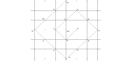
Figure 1. $\circ=\Gamma_{0}$, $\bullet=\Gamma_{1}$

We start by denoting $a_{1},a_{2},a_{3},a_{4}$ the neighbours of $(0,0)$. Obviously, since $(0,0)\in\Gamma_{0}$, the nodes $a_{i}\in\Gamma_{1}$ for $i=1,...,4$. After choosing $a_{1}$ from any of the four neighbours, the rest are named clockwise. Then, we choose $a_{5}$ to be any of the nodes in $\Gamma_{1}$ of distance two from $a_{4}$ and distance three from $(0,0)$. We continue in the same manner clockwise the enumeration of the rest of the nodes in $\Gamma_{1}$ that have distance three from $(0,0)$, then distance four, and so on. In this way we construct a spiral comprising of the nodes in $\Gamma_{1}$ always moving clockwise while we move away from $(0,0)$. We can then write $\mathbb{E}^{\Gamma_{1}}=\sqcap_{i=1}^{+\infty}\ \mathbb{E}^{a_{i}}$. Since we have obtain in Proposition 5.1 a log-Sobolev inequality for the one node measure, we will express the entropy of the product measure $\mathbb{E}^{\Gamma_{1}}$ in terms of the individual entropies as seen below

(6.9) $$\nu\mathbb{E}^{\Gamma_{1}}(f^{2}\log\frac{f^{2}}{\mathbb{E}^{\Gamma_{1}}f^{2}})=\sum_{k=1}^{+\infty}\nu\mathbb{E}^{a_{k}}(\mathbb{E}^{a_{k-1}}...\mathbb{E}^{a_{1}}f^{2}\log\frac{\mathbb{E}^{a_{k-1}}...\mathbb{E}^{a_{1}}f^{2}}{\mathbb{E}^{a_{k}}...\mathbb{E}^{a_{1}}f^{2}})$$

so that we can upper bound the one site entropies from the log-Sobolev inequalities,

(6.10) $$\nu\mathbb{E}^{a_{k}}(\mathbb{E}^{a_{k-1}}...\mathbb{E}^{a_{1}}f^{2}\log\frac{\mathbb{E}^{a_{k-1}}...\mathbb{E}^{a_{1}}f^{2}}{\mathbb{E}^{a_{k}}...\mathbb{E}^{a_{1}}f^{2}})\leq c_{1}\nu\|\nabla_{a_{k}}\ f\|^{2}+c_{2}\sum_{j\sim a_{k}}\nu\|\nabla_{j}(\mathbb{E}^{a_{k-1}}...\mathbb{E}^{a_{1}}f^{2})^{\frac{1}{2}}\|^{2}$$

where above in the computation of the first term we used that $a_{i}$’s have distance bigger than one from each other, and so $\nu\|\nabla_{a_{k}}(\mathbb{E}^{a_{k-1}}...\mathbb{E}^{a_{1}}f^{2})^{\frac{1}{2}}\|^{2}\leq\nu\|\nabla_{a_{k}}f\|^{2}$. For the second summand in (6.10) notice that the neighbours of $a_{k}$ can be distinguished into two categories. Those that have distance bigger than one from $a_{k-1},a_{k-2},...,a_{1}$ and those that neighbour with at least one of $a_{k-1},a_{k-2},...,a_{1}$. For $j\sim a_{k}$ that belong to the first category, since they do not neighbour any of the nodes $a_{k-1},a_{k-2},...,a_{1}$ we clearly get

(6.11) $$\nu\|\nabla_{j}(\mathbb{E}^{a_{k-1}}...\mathbb{E}^{a_{1}}f^{2})^{\frac{1}{2}}\|^{2}\leq\nu\|\nabla_{j}f\|^{2}$$

For those neighbours of $a_{k}$, that neighbour with at least one of the $a_{k-1},a_{k-2},...,a_{1}$ we can write

$$\nu\|\nabla_{j}(\mathbb{E}^{a_{k-1}}...\mathbb{E}^{a_{1}}f^{2})^{\frac{1}{2}}\|^{2}\leq\Phi(j)$$

If we bound this by (6.8)

(6.12) $$\nu\|\nabla_{j}(\mathbb{E}^{a_{k-1}}...\mathbb{E}^{a_{1}}f^{2})^{\frac{1}{2}}\|^{2}\leq R_{3}\Theta(j)$$

Gathering together (6.12), (6.11) and (6.10) we have

$$\nu\mathbb{E}^{a_{k}}(\mathbb{E}^{a_{k-1}}...\mathbb{E}^{a_{1}}f^{2}\log\frac{\mathbb{E}^{a_{k-1}}...\mathbb{E}^{a_{1}}f^{2}}{\mathbb{E}^{a_{k}}...\mathbb{E}^{a_{1}}f^{2}})\leq c_{1}\nu\|\nabla_{a_{k}}f\|^{2}+c_{2}\sum_{j\sim a_{k}}\nu\|\nabla_{j}f\|^{2}+$$

$$+c_{2}R_{3}\sum_{j\sim a_{k}}\Theta(j)$$

Then, if we combine this bound together with (6.9) we obtain

$$\nu\mathbb{E}^{\Gamma_{1}}(f^{2}\log\frac{f^{2}}{\mathbb{E}^{\Gamma_{1}}f^{2}})\leq c_{1}\sum_{k=1}^{+\infty}\nu\|\nabla_{a_{k}}f\|^{2}+c_{2}\sum_{k=1}^{+\infty}\sum_{j\sim a_{k}}\nu\|\nabla_{j}f\|^{2}+$$

$$+c_{2}R_{3}\sum_{k=1}^{+\infty}\sum_{j\sim a_{k}}\sum_{n=0}^{2}\sum_{r:dist(s,j)=n}\ \nu\|\nabla_{s}f\|^{2}$$

If we notice that for every node there are four nodes at distance one and eight at distance two, after rearranging the sums above we finally obtain

$$\nu\mathbb{E}^{\Gamma_{1}}(f^{2}\log\frac{f^{2}}{\mathbb{E}^{\Gamma_{1}}f^{2}})\leq(c_{1}+13R_{3}c_{2})\nu\|\nabla_{\Gamma_{1}}f\|^{2}+(4c_{2}+13R_{3}c_{2})\nu\|\nabla_{\Gamma_{0}}f\|^{2}$$

∎∎

7. The log-Sobolev inequality for the Gibbs measure

In this section we prove the main result stated in Theorem 2.1. We recall that $\mathbb{Q}^{n}$ is defined as $\mathbb{Q}^{0}f=f$ and $\mathbb{Q}^{n}:=\mathbb{E}^{\Gamma_{0}}\mathbb{Q}^{n-1}$ when $n$ is odd and $\mathbb{Q}^{n}:=\mathbb{E}^{\Gamma_{1}}\mathbb{Q}^{n-1}$ when $n$ is even.

Proof.

If $\Lambda$ is a subset of $\mathbb{Z}^{d}$, we write $\operatorname{\mathsf{Ent}}_{\mathbb{E}^{\Lambda}}$ for the entropy of the probability measure $\mathbb{P}^{\Lambda,\omega}$ on $\mathsf{S}^{\Lambda}$, that is, $\operatorname{\mathsf{Ent}}_{\mathbb{E}^{\Lambda}}(g)=\mathbb{E}^{\Lambda}\big{[}g\log\frac{g}{\mathbb{E}^{\Lambda}g}\big{]}$. From this, with $\lambda(x):=x\log x$, we have

(7.1) $$\mathbb{E}^{\Lambda}[\lambda(g)]=\operatorname{\mathsf{Ent}}_{\mathbb{E}^{\Lambda}}(g)+\lambda(\mathbb{E}^{\Lambda}g),$$

where we used the fact that $\mathbb{E}^{\Lambda}g$ does not depend on $x_{\Lambda}$.

We claim that, for all $n\geq 1$,

$$\mathbb{Q}^{n}[\lambda(g)]= \sum_{m=0,\ m\ \text{odd}}^{n-1}\mathbb{Q}^{n-m-1}\mathbb{E}^{\Gamma_{1}}[\operatorname{\mathsf{Ent}}_{\mathbb{E}^{\Gamma_{0}}}(\mathbb{Q}^{m}g)]+\sum_{m=0,\ m\ \text{even}}^{n-1}\mathbb{Q}^{n-m-1}[\operatorname{\mathsf{Ent}}_{\mathbb{E}^{\Gamma_{1}}}(\mathbb{Q}^{m}g)]+$$

(7.2) $$+\lambda(\mathbb{Q}^{n}g).$$

To see this, notice first that the statement is trivial for $n=1$. Assuming it true for some $n\geq 1$, we prove the same thing with $n+1$ in place of $n$. Apply (7.1) with $\Lambda=\Gamma_{0}$ and $\mathbb{Q}^{n}g$ for $n$ odd in place of $g$:

$$\mathbb{E}^{\Gamma_{0}}[\lambda(\mathbb{Q}^{n}g)]=\operatorname{\mathsf{Ent}}_{\mathbb{E}^{\Gamma_{0}}}(\mathbb{Q}^{n}g)+\lambda(\mathbb{E}^{\Gamma_{0}}\mathbb{Q}^{n}g),$$

and, again from (7.1) with $\Lambda=\Gamma_{1}$ and $\mathbb{Q}^{n}g$ for $n$ even in place of $g$,

$$\mathbb{E}^{\Gamma_{1}}[\lambda(\mathbb{Q}^{n}g)]=\operatorname{\mathsf{Ent}}_{\mathbb{E}^{\Gamma_{1}}}(\mathbb{Q}^{n}g)+\lambda(\mathbb{E}^{\Gamma_{1}}\mathbb{Q}^{n}g).$$

From the last two displays, for odd $n$ we get

$$\mathbb{E}^{\Gamma_{1}}[\lambda(\mathbb{Q}^{n}g)]=\mathbb{E}^{\Gamma_{1}}[\operatorname{\mathsf{Ent}}_{\mathbb{E}^{\Gamma_{0}}}(\mathbb{Q}^{n}g)]+\operatorname{\mathsf{Ent}}_{\mathbb{E}^{\Gamma_{1}}}(\mathbb{E}^{\Gamma_{0}}\mathbb{Q}^{n}g)+\lambda(\mathbb{Q}^{n+1}g)$$

while for $n$ even

$$\mathbb{E}^{\Gamma_{0}}[\lambda(\mathbb{Q}^{n}g)]=\mathbb{E}^{\Gamma_{0}}[\operatorname{\mathsf{Ent}}_{\mathbb{E}^{\Gamma_{1}}}(\mathbb{Q}^{n}g)]+\operatorname{\mathsf{Ent}}_{\mathbb{E}^{\Gamma_{0}}}(\mathbb{E}^{\Gamma_{1}}\mathbb{Q}^{n}g)+\lambda(\mathbb{Q}^{n+1}g)$$

Using these, and applying $\mathbb{E}^{\Gamma_{0}}$ or $\mathbb{E}^{\Gamma_{1}}$ to (7) when $n$ is even or odd respectively, we readily obtain (7) with $n+1$ in place of $n$. This shows the veracity of (7). Using Lemma 4.4, we have $\mathbb{Q}^{n}[\lambda(g)]\to\nu[\lambda(g)]$ and $\lambda^{n}(\mathbb{Q}^{n}g)\to\nu[g]$, $\nu$-a.e. From this and Fatou’s lemma, (7) gives

$$\operatorname{\mathsf{Ent}}_{\nu}(g) \leq\varliminf_{n\to\infty}\bigg{\{}\nu\bigg{[}\sum_{m=0,\ m\ \text{odd}}^{n-1}\mathbb{Q}^{n-m-1}[\operatorname{\mathsf{Ent}}_{\mathbb{E}^{\Gamma_{0}}}(\mathbb{Q}^{m}g)]+\sum_{m=0,\ m\ \text{even}}^{n-1}\mathbb{Q}^{n-m-1}[\operatorname{\mathsf{Ent}}_{\mathbb{E}^{\Gamma_{1}}}(\mathbb{E}^{\Gamma_{0}}\mathbb{Q}^{m}g)]\bigg{]}\bigg{\}},$$

(7.3) $$=\varliminf_{n\to\infty}\bigg{\{}\sum_{{}^{m=0,\ m\ \text{odd}}}^{n-1}\nu[\operatorname{\mathsf{Ent}}_{\mathbb{E}^{\Gamma_{0}}}(\mathbb{Q}^{m}g)]+\sum_{m=0,\ m\ \text{even}}^{n-1}\nu[\operatorname{\mathsf{Ent}}_{\mathbb{E}^{\Gamma_{1}}}(\mathbb{E}^{\Gamma_{0}}\mathbb{Q}^{m}g)]\bigg{\}}$$

where we used the fact that $\nu$ is a Gibbs measure to obtain the last equality. Let $g=f^{2}$ and apply Proposition 6.4 to bound the entropy

$$\nu[\operatorname{\mathsf{Ent}}_{\mathbb{E}^{\Gamma_{0}}}(\mathbb{Q}^{m}f^{2})] \leq\tilde{C}\nu\|\nabla_{\Gamma_{0}}\sqrt{\mathbb{Q}^{m}f^{2}}\|^{2}\leq\tilde{C}[C_{1}C_{2}^{m-1}\nu\|\nabla_{\Gamma_{1}}f\|^{2}+\tilde{C}C_{2}^{m}\nu\|\nabla_{\Gamma_{0}}f\|^{2}]$$

$$\nu[\operatorname{\mathsf{Ent}}_{\mathbb{E}^{\Gamma_{1}}}(\mathbb{E}^{\Gamma_{0}}\mathbb{Q}^{m}f^{2})] \leq\tilde{C}\nu\|\nabla_{\Gamma_{1}}\sqrt{\mathbb{E}^{\Gamma_{0}}\mathbb{Q}^{m}f^{2}}\|^{2}\leq\tilde{C}[C_{1}C_{2}^{m-1}\nu\|\nabla_{\Gamma_{0}}f\|^{2}+\tilde{C}C_{2}^{m}\nu\|\nabla_{\Gamma_{1}}f\|^{2}],$$

for $m$ odd and even respectively, where, for the last inequalities we used Lemma 6.3 and induction. Substituting in (7.3), we obtain (recall that $0<C_{2}<1$)

$$\operatorname{\mathsf{Ent}}_{\nu}(f^{2})\leq\frac{\tilde{C}(C_{1}C_{2}^{-1}+C_{2})}{1-C_{2}}\nu\|\nabla_{\Gamma_{1}}f\|^{2}+\frac{\tilde{C}(C_{1}C_{2}^{-1}+C_{2})}{1-C_{2}}\nu\|\nabla_{\Gamma_{0}}f\|^{2}\leq\overline{C}\,\nu\|\nabla f\|^{2},$$

where $\overline{C}$ is the largest of the two coefficients. This is the log-Sobolev inequality for $\nu$. ∎∎

8. Example

We consider the Hamiltonian for a measure on the Heisenberg group defined as in (2.13). Theorem 2.5 follows from the main result presented in Theorem 2.1. Thus, we need to verify that the conditions of Theorem 2.1 are satisfied for a local specification with a Hamiltonian as in (2.13).

At first, we need to verify that the main hypothesis, that the single site measure without interactions (consisting only of the phase) $\mu(dx)=\frac{e^{-\varphi(x)}dx}{\int e^{-\varphi(x)}dx}$ satisfies the log-Sobolev inequality. In our example where $\varphi(x)=\bm{d}(x)^{p},p>2$, as explained in the introduction in section 1.2, this is true, since the family of measures (1.1) satisfies the log-Sobolev inequality, a result that has been proven in [H-Z]. Furthermore, hypothesis (2.3) and (2.4) about the Carnot-Carathéodory distance on the Heisenberg group $\mathbb{H}_{1}$ are true (see [Mo] and [H-Z]).

At first one notices, that for convenience the interaction potential can be written in the following equivalent form:

(8.1) $$V(x,\omega)=\delta\bm{d}^{r}(x)+\sum_{k=1}^{r-1}a_{k}\bm{d}^{r-k}(x)\bm{d}^{k}(\omega)$$

where $a_{k}=\begin{pmatrix}r\\ k\\ \end{pmatrix}$ the binomial coefficients.

For conditions (2.10) - (2.12), the first one easily follows from $\bm{d}^{r}(xz)\leq 2^{r-1}\bm{d}(x)+2^{r-1}\bm{d}(z)$ for every $r\in\mathbb{N}$ and the specific form of $\varphi$ and $V$. The second and third plausibly from $\bm{d}(x^{-1})=\bm{d}(x)$ and $\bm{d}(\gamma(s))\leq\bm{d}(z)$ for any geodesic from $0$ to $z$, both by the definition of the Carnot-Carathéodory distance.

Finally, conditions (2.1)-(2.2) and (2.5)-(2.9) can easily be verified for any $s=2p-2$ and $r\leq\frac{p+2}{2}$, if one writes the interaction potential in the form (8.1).

References

- [A-B-C] C. Ané, S. Blachère, D. Chafaï, P. Fougères, I. Gentil, F. Malrieu, C. Roberto and G. Scheffer, Sur les inégalités de Sobolev logarithmiques, Panoramas et Synthèses. Soc. Math, 10, France, Paris (2000).
- [B-E] D. Bakry and M. Emery, Difusions hypercontractives ,Seminaire de Probabilites XIX, Springer Lecture Notes in Math. 1123, 177-206 (1985).
- [Ba-En-Hu-Ma] Z.M. Balogh, A. Engulatov, L. Hunziker and O. E. Maasalo, Functional Inequalities and Hamilton–Jacobi Equations in Geodesic Spaces, Potential Anal, 36, 401-432 (2012)
- [BA-Bo12] F. Baudoin and M. Bonnefont, Log-Sobolev inequalities for subelliptic operators satisfying a generalized curvature dimension inequality, J of Funct Analysis, 262, 2646-2676 (2012)
- [B-HK] J. Bellisard and R. Hoegn-Krohn, Compactness and the maximal Gibbs state for random fields on the Lattice, Commun. Math. Phys., 84, 297-327 (1982).
- [B-G] S.G. Bobkov and F. Gotze, Exponential integrability and transportation cost related to logarithmic sobolev inequalities , J of Funct Analysis 163 1-28 (1999).
- [B-L-U] A. Bonfiglioni, E. Lanconelli and F. Uguzzoni, Stratified Lie groups and Potential Theory for their Sub-Laplacians, Springer Monographs in Mathematics. Springer, New York (2007).
- [Bo-Ch-He] M. Bonnefont, D. Chafaï and R. Herry, On logarithmic Sobolev inequalities for the heat kernel on the Heisenberg group Ann. Fac. Sci. Toulouse Math., 29, 335-355 (2020).
- [B-Z] S.G. Bobkov and B. Zegarlinski, Entropy Bounds and Isoperimetry. Memoirs of the American Mathematical Society, Vol: 176, 1 - 69 (2005).
- [B-H] T. Bodineau and B. Helffer, Log-Sobolev inequality for unbounded spin systems , J of Funct Analysis 166, 168-178 (1999).
- [Ch-Ka-Ru] M. Chatzakou and A. Kassymov and M. Ruzhansky, Logarithmic Sobolev inequalities on Lie groups. , arXiv:2106.15652 (2021).
- [Da-Ze] E.B. Dagher and B. Zegarlinski, Coercive Inequalities and U-Bounds on Step-Two Carnot Groups., Potential Anal 59, 589–612 (2021).
- [Da22] E.B. Dagher, Note on the q-logarithmic Sobolev and p-Talagrand inequalities on Carnot groups. Commun. Contemp. Math. (2022).
- [Da-Qi-Ze] E.B. Dagher and Y. Qiu and B. Zegarlinski and M. Zhang, Spectral Gap Inequalities on Nilpotent Lie Groups in Infinite Dimensions. , arXiv:2211.14188 (2022).
- [D] R. L. Dobrushin, The problem of uniqueness of a Gibbs random field and the problem of phase transition, Funct. Anal. Apll. 2, 302-312 (1968).
- [Fe-Li] Q. Feng and W. Li, Entropy dissipation for Degenerate Stochastic Differential Equations via Sub-Riemannian Density Manifold, Entropy, 25 (2023).
- [Fe-Li1] Q. Feng and W. Li, Sub-Riemannian Ricci curvature via generalized Gamma z calculus, arXiv:2004.01863 (2020).
- [Ge-Gu-M-05] I. Gentil, A. Guillin and L. Miclo, Modified logarithmic Sobolev inequalities and transportation inequalities,Probab. Theory Relat. Fields, 133, 409-436 (2005).
- [Ge-Gu-M-07] I. Gentil, A. Guillin and L. Miclo, Modified logarithmic Sobolev inequalities in null curvature, Rev. Mat. Iberoamericana, 23, 235-258 (2007).
- [G-R] I. Gentil and C. Roberto, Spectral Gaps for Spin Systems: Some Non-convex Phase Examples, J. Func. Anal., 180, 66-84 (2001).
- [Gor-Luo] M. Gordina and L. Luo, Logarithmic Sobolev inequalities on non-isotropic Heisenberg groups, J. Func. Anal., 283, 66-84 (2022).
- [Go-Ro-Sa] N. Gozlan and C. Roberto and P.-M. Samson, Characterization of Talagrand’s Transport-Entropy inequalities in metric spaces. .Ann. Probab, 5, 3112–3139 (2013).
- [G] L. Gross, Logarithmic Sobolev inequalities, Am. J. Math. 97, 1061-1083 (1976).
- [G-Z] A.Guionnet and B.Zegarlinski, Lectures on Logarithmic Sobolev Inequalities. IHP Course 98, Seminare de Probabilite XXVI, Lecture Notes in Mathematics 1801, 1-134, Springer (2003).
- [H-Z] W.Hebisch and B.Zegarlinski, Coercive inequalities on metric measure spaces. J. Func. Anal., 258, 814-851 (2010).
- [H] B. Helffer, Semiclassical Analysis, Witten Laplacians and Statistical Mechanics, World Scientific, Singapore (2002).
- [I-K-Z11] J. Inglis and V. Kontis and B. Zegarliński, From U-bounds to isoperimetry with applications to H-type groups. J. Func. Anal., 260, 76-116 (2011).
- [I-P1] J. Inglis and I. Papageorgiou, Log-Sobolev inequalities for infinite-dimensional Gibbs measures with non-quadratic interactions. Markov Proc. Related Fields, 25, 879-898 (2019).
- [I-P] J. Inglis and I. Papageorgiou, Logarithmic Sobolev Inequalities for Infinite Dimensional Hörmander Type Generators on the Heisenberg Group. Potential Anal., 31, 79-102 (2009).
- [Ch-Fe-Ze1] M. Chatzakou, S. Federico and B. Zegarlinski, Poincaré inequalities on Carnot Groups and spectral gap of Schrödinger operators.arXiv:2211.09471 (2023).
- [Ch-Fe-Ze2] M. Chatzakou, S. Federico and B. Zegarlinski, q-Poincare inequalities on Carnot Groups with filiform type Lie algebra. Potential Anal. (2023).
- [KOZ2] V. Kontis and M. Ottobre and B. Zegarlinski, Markov semigroups with hypocoercive-type generator in infinite dimensions: Ergodicity and smoothing. J. Func. Anal., 270, 3173-3223 (2016).
- [KOZ1] V. Kontis and M. Ottobre and B. Zegarlinski, Long- and short-time behaviour of hypocoercive-type operators in infinite dimensions: An analytic approach. Infin. Dimens. Anal. Quantum Probab., 20 (2017).
- [Led] M. Ledoux, Logarithmic Sobolev inequalities for unbounded spin systems revisited. Seminaire de Probabilites XXXV. Lecture Notes in Math. 1755, 1167-194. Springer (2001).
- [M1] K. Marton, An inequality for relative entropy and logarithmic Sobolev inequalities in Eucledian spaces. J. Func. Anal., 264, 34-61 (2013).
- [Mo] R. Monto, Some properties of Carnot-Carathéodory balls in the Heisenberg group. , Rend. Mat. Acc. Lincei, 11, 155-167 (2007).
- [O-R] F. Otto and M. Reznikoff, A new criterion for the Logarithmic Sobolev Inequality and two Applications , J. Func. Anal., 243, 121-157 (2007).
- [Pa3] I. Papageorgiou, The log-Sobolev inequality with quadratic interactions., J. Math. Phys., 59 (2018).
- [Pa2] I. Papageorgiou, The logarithmic Sobolev inequality for Gibbs measures on infinite product of Heisenberg groups. Markov Proc. Related Fields, 20, 705-749 (2014).
- [Pa1] I. Papageorgiou, The Logarithmic Sobolev Inequality in Infinite dimensions for Unbounded Spin Systems on the Lattice with non Quadratic Interactions, Markov Proc. Related Fields, 16, 447-484 (2010).
- [Pa4] I. Papageorgiou, Concentration inequalities for Gibbs measures, Infin. Dimens. Anal. Quantum Probab. Relat., 14, 79-104 (2011).
- [Pa5] I. Papageorgiou, A note on the modified Log-Sobolev inequality., J. Potential Anal. 35, 275-286 (2011).
- [Pr] C.J.Preston,Random Fields, LNM 534, Springer (1976).
- [R-Z] C. Roberto and B. Zegarlinski, Orlicz-Sobolev inequalities for sub-Gaussian measures and ergodicity of Markov semi-groups , J. Func. Anal., 243 (1), 28-66 (2007).
- [R] O. Rothaus, Analytic inequalities, isoperimetric inequalities and logarithmic Sobolev inequalities, J. Func. Anal., 64, 296-313 (1985).
- [SC] L.Saloff-Coste, Aspects of Sobolev-Type Inequalities, London Mathematical Society Lecture Note Series, 289. Cambridge University Press, Cambridge, (2002).
- [V-SC-C] N. Th. Varopoulos, L. Saloff-Coste and T. Coulhon, Analysis and Geometry on Groups, Tracts in Mathematics, 100, Cambridge University Press, Cambridge, (1992).
- [Won] Y.S. Won, An L2-approximation method for construction andsmoothing estimates of Markov semigroups forinteracting diffusion processes on a lattice, Infin. Dimens. Anal. Quantum Probab. Relat. 24 (2021).
- [Y] N.Yoshida, The log-Sobolev inequality for weakly coupled lattice field, Probab.Theor. Relat. Fields 115, 1-40 (1999).
- [Z1] B. Zegarlinski, On log-Sobolev Inequalities for Infinite Lattice Systems, Lett. Math. Phys. 20, 173-182 (1990).
- [Z2] B. Zegarlinski, The strong decay to equilibrium for the stochastic dynamics of unbounded spin systems on a lattice, Comm. Math. Phys. 175, 401-432 (1996).