Are the XYZ states unconventional states or conventional states with unconventional properties?

Abstract

We discuss three possible scenarios for the interpretation of mesons containing a heavy quark and its antiquark near and above the first threshold for a decay into a pair of heavy mesons in a relative $S$–wave. View I assumes that these thresholds force the quark potential to flatten which implies that while in these energy ranges molecular states may be formed there should not be any quark–anti-quark states above these thresholds. View II assumes that the main part of the interaction between two mesons is due to the poles which originate from the $Q\bar{Q}$ interaction. The properties of the $Q\bar{Q}$ mesons are strongly influenced by opening thresholds but the number of states is given by the quark model. In View III, both types of mesons are admitted also near and above the open flavor thresholds: $Q\bar{Q}$ mesons and dynamically generated mesons. Experimental consequences of these different views are discussed.

I Introduction

Great progress has been achieved in the spectroscopy of hadrons containing two heavy quarks due to the tremendous efforts of experiments like BaBar, Belle, BESIII, CLEO, LHCb, $\cdots$, and further progress is expected from the ongoing programs and, in the future, from Belle II and PANDA. At present, the Particle Data Group (PDG) Tanabashi:2018oca lists 37 states containing a $c\bar{c}$ and 20 states containing a $b\bar{b}$ pair. Amongst those there are many states with unexpected properties, like footnote1 $\chi_{c1}(3872)$ also known as (aka) $X(3872)$, $\psi(4260)$ aka $Y(4260)$, $\psi(4360)$ aka $Y(4360)$, $\psi(4660)$ aka $Y(4660)$, and $\chi_{c1}(4140)$ and $\chi_{c1}(4274)$. Moreover, there are even states with isospin $I=1$ (established are $Z_{c}(3900)$, $Z_{c}(4020)$, $Z_{c}(4430)$, $Z_{b}(10610)$, $Z_{b}(10650)$) decaying to final states that contain a heavy quark and its antiquark — as such the states must contain at least four quarks. All these states are classified as unconventional states or as candidates for an exotic structure, but it is unclear what their underlying structure is.

In the literature those states are typically proposed to be quarkonia ($Q\bar{Q}$), possibly with unconventional properties, compact tetraquarks (diquark—antidiquark $(qQ)$-$(\bar{Q}\bar{q})$), hybrids ($\bar{Q}Q$ states with active gluons contributing to the quantum numbers), hadroquarkonia (with a structure as ($Q\bar{Q}$)-($q\bar{q}$)), or loosely bound molecular states ($Q\bar{q}$)-($Q\bar{q}$). A large number of reviews has appeared recently that discuss the exotic candidates from different angles, see, e.g., Refs. Brambilla:2010cs ; Esposito:2016noz ; Chen:2016qju ; Ali:2017jda ; Lebed:2016hpi ; Olsen:2017bmm ; Guo:2017jvc . The key issue is if in the presence of light quarks the heavy quark–antiquark potential keeps rising as it does in the quenched approximation of the potential. This would imply that near and above the first relevant $S$–wave open flavor threshold at most molecular states could exist but no quark–anti-quark states. It should be stressed that many unexpected phenomena were discovered very close to important thresholds.

The problem at hand is probably best explained by a brief look at $\chi_{c1}(3872)$. Its very small binding energy (there is currently only an upper limit of 180 keV for this binding energy) makes this state a prime example of a loosely bound molecule. However, the question remains, if this state is just a molecule produced by two-hadron interactions or if it owes it existence a $c\bar{c}$ core. The $\chi_{c1}(2P)$ may still be waiting for discovery — or it is already found and should be identified with the $\chi_{c1}(4140)$. The pattern of the $\chi_{c}(1P)$ states suggests that the three states $\chi_{c2}(3930)$, $\chi_{c1}(3872)$, $\chi_{c0}(3860)$ could be the $\chi_{c}(2P)$ states. In this paper, we compare the implications of three very different hypotheses regarding the doubly heavy states near or above the first relevant open heavy flavor threshold.

View I underlines the importance of the “molecular” interaction between two mesons. In this view, the $\chi_{c1}(3872)$ is an isoscalar $D^{*}\bar{D}+c.c.$ molecule unrelated to the $c\bar{c}$ system. (The charge conjugated component is omitted from now onwards.) Here, as in all partial waves, quarkonia exist only below the first relevant $S$-wave threshold for a two-particle decay — this statement implies that these two particles must be narrow, $\Gamma\ll\Lambda_{\rm QCD}$, for otherwise the possible molecule would be too broad Filin:2010se or, stated differently, would have already decayed before it could hadronize Guo:2011dd . In this view it is assumed that at this threshold virtual light quarks screen the quark-antiquark potential. As a result the potential flattens off and all resonances at or above the threshold are of molecular nature. In this scenario, $Q\bar{Q}$ states exist only below this threshold, and the number of molecular states is (at most) given by the number of relevant $S$–wave thresholds in the kinematic range of interest (although there might also be $P$–wave states observed already — this is discussed below). Note that not necessarily all $S$–wave channels have a sufficiently strong attractive interaction to generate singularities with a significant impact on observables (Note that in the two nucleon sector there is a bound state only in the spin triplet, isospin singlet channel. In the spin singlet, isospin triplet channel there is only a virtual state which is, however, so close to the threshold that it generates a very large scattering length).

View II is based on the assumption that the leading part of the interaction between two mesons is due to their $Q\bar{Q}$ component. The argument is that there can be different reasons to expect a resonance in a given mass range. Mesons with a given set of quantum numbers can be $q\bar{q}$, they could be hybrids (abbreviated often as $q\bar{q}g$), tetraquarks $qq\bar{q}\bar{q}$, molecular meson-meson resonances, baryonia (baryon-antibaryon bound states or resonances) or glueballs. These are six different possible species. However, there is no experimental evidence for such an abundance. View II assumes that these different ingredients may be components in the mesonic wave function, but that these options do not manifest themselves in separate resonances. In this view, the number of expected heavy-quark states is given by the number of expected $Q\bar{Q}$ states. It is assumed that these states drive the major part of the interactions between the particles into which the states decay. Due to threshold openings, the properties of the wave function can change as well as the resonance parameters but not the number of states. In this view, $\chi_{c1}(3872)$ would have a $\bar{Q}Q$ and a sizeable molecular component. But there is one $\chi_{c1}$ state only in this mass range that should be identified with $\chi_{c1}(2P)$.

One can in principle also think of a mixture of View I and II, if one were to admit that deuteron-like loosely bound states of two hadrons might exist if there is no possibility to reduce the number of quarks. In this formulation, exotic mesons like the $Z$ particles ($Z_{c}(3900)$, $Z_{b}(10610)$, $\cdots$) might exist as poles of the $S$–matrix. However, we will not go deeper into this discussion here.

Finally, in View III, we allow for the existence of both even above the first relevant two–hadron threshold: States that owe their existence their $\bar{Q}Q$ core as well as those that are of molecular nature. In this scenario the number of states will exceed the number of states defined by the $\bar{Q}Q$ model. Moreover, one expects states near $S$–wave thresholds as well as states with masses unrelated to those.

In principle the same issues raised above could also be discussed for the light quark sector, however, due to the non-perturbative nature of QCD at small momentum transfers but asymptotic freedom at large scales, one expects that heavy–heavy systems, which are the focus of this work, are easier to analyse than heavy–light or all–light systems. Moreover, the heavy quark spin symmetry (HQSS) states that, up to corrections of order $\Lambda_{\rm QCD}/M_{Q}$ where $\Lambda_{\rm QCD}\simeq 200$ MeV denotes the QCD mass scale and $M_{Q}$ the heavy quark mass, the heavy quark spin does not interact. This results in the appearance of spin multiplets and allows one to identify selection rules for certain decays that are sensitive to the internal structure of the states, both of which proved to be important diagnostic tools when it comes to classifying exotic states. In addition, mesons have an easier substructure than baryons. Thus in what follows we focus on doubly heavy mesonic systems.

II The bottomonium spectrum

Fig. 1 shows the spectrum in the b-quark sector. The spectrum is very clean. There is a series of $\Upsilon$ states, $\Upsilon(1S)\cdots\Upsilon(4S)$ footnote2 , $\Upsilon(10860)$ and $\Upsilon(11020)$, with quantum numbers $I^{G}(J^{PC})=0^{+}(1^{--}$) where $I$, $G$, $J$, $P$, $C$ are the isospin, G-parity, total spin, parity and C-parity of the mesons. The vector states can be produced in $e^{+}e^{-}$ annihilation, and most of our detailed knowledge on the $\Upsilon$-family of states stems from this process. The $\Upsilon(n^{3}D_{1})$ states have the same quantum numbers as the $\Upsilon(nS)$ states and could in principle be produced in $e^{+}e^{-}$ annihilation as well, but this production violates spin symmetry which is most probably the reason why those have not been seen here. The $\Upsilon(1^{3}D_{2})$ state (with orbital angular momentum $L=2$ and quark spin $S=1$) has been seen in a $\Upsilon(3S)\to\gamma\chi_{b}(2P)$, $\chi_{b}(2P)\to\gamma\Upsilon(1^{3}D_{2})$, $\Upsilon(1^{3}D_{2})\to\gamma\chi_{b}(1P)$, $\chi_{b}(1P)\to\gamma\Upsilon(1S)$ cascade decay with four photons in the final state Bonvicini:2004yj .

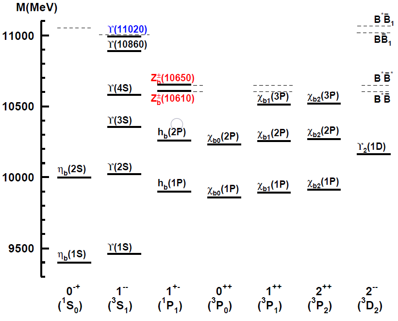
Figure 1: (Color online) The bottomonium states. Established states are given by a solid line and their names. The thresholds for $S$-wave decays in each channel are indicated by dashed lines. The $1^{++}$ and $1^{+-}$ partial waves have their $S$-wave threshold at the $B^{*}\bar{B}$, the $2^{++}$ partial wave at the $B^{*}\bar{B}^{*}$ threshold. In View I, states close to or above thresholds (in blue) and the isospin 1 states (in red) are interpreted as molecular states. In View II only states compatible with $Q\bar{Q}$ exist.

The two resonances $\Upsilon(10860)$ and $\Upsilon(11020)$ are above the open beauty threshold — given the quantum numbers, the decay $\Upsilon\to B^{(*)}\bar{B}^{(*)}$ happens in a $P$-wave. The mass of the $\Upsilon(11020)$ is right below the first $S$-wave threshold, namely $B_{1}\bar{B}$, where $B_{1}$ denotes the axial vector $B$-meson with the light quark cloud carrying $j=3/2$.

Further states are known: There are two pseudoscalar mesons, $\eta_{b}(1S)$ and $\eta_{b}(2S)$. They are found slightly below the corresponding vector states in line with expectations from HQSS for $\bar{b}b$ states. In addition, there are two complete quartets with $L=1$; two spin triplets $\chi_{bJ}(nP)$ with $J=0,1,2$ and $n=1,2$ and two spin singlets $h_{b}(nP)$, again with $n=1,2$. Two states belong to the $3P$ series: $\chi_{b1}(3P)$ and the recently discovered $\chi_{b2}(3P)$ Sirunyan:2018dff .

The spin-triplet and spin-singlet states satisfy the center-of-gravity rule which holds true when tensor and spin-spin forces are negligible:

$$M_{h_{Q}(nP)}=\frac{1}{9}\left(5M_{\chi_{Q2}(nP)}+3M_{\chi_{Q1}(nP)}+M_{\chi_{Q0}(nP)}\right)$$ (1)

For $Q$ = $b,n$ = 1, the difference between the left hand side and the right hand side is $\delta M$ = -(0.57$\pm$1.08) MeV and for $Q$ = $b,n$ = 2, $\delta M$ = $-(0.4\pm 1.3)$ MeV. The center-of-gravity rule is excellently satisfied.

Note that with the exception of $\Upsilon(11020)$ all states discussed so far are well below the threshold for $S$-wave decays. The pertinent thresholds for the different quantum numbers for $S$-wave decays are shown in Table 1.

Table 1: The lowest $S$–wave thresholds for a given $J^{PC}$, shown in the first line.

$0^{-+}$	$1^{--}$	$1^{+-}$	$0^{++}$	$1^{++}$	$2^{++}$	$2^{--}$
$B_{1}\bar{B}^{*}$	$B_{1}\bar{B}$	$B^{*}\bar{B}$	$B\bar{B}$	$B^{*}\bar{B}$	$B^{*}\bar{B}^{*}$	$B_{2}\bar{B}$
11.050	11.004	10.604	10.558	10.604	10.650	11.019

The two isotriplets of states $Z_{b}(10610)$ and $Z_{b}(10650)$ with quantum numbers $1^{+}(1^{-+})$ are evidently not $b\bar{b}$ mesons and have no pure $b\bar{b}$ component. The minimal quark content for a $Z_{b}^{+}$ is $b\bar{b}u\bar{d}$ with four quarks suggesting a tetraquark configuration Ali:2011ug . However, $Z_{b}(10610)$ and $Z_{b}(10650)$ decay not only into bottomonium states, they also decay into pairs of mesons with open bottomness: $Z_{b}(10610)$ with a fraction of $(82.6\pm 2.9\pm 2.3)$% into $\bar{B}B^{*}$, and $Z_{b}(10650)$ with $(70.6\pm 4.9\pm 4.4)$% into $\bar{B}^{*}B^{*}$ (but not into $\bar{B}B^{*}$). Thus a molecular nature of $Z_{b}(10610)$ and $Z_{b}(10650)$ is very likely Bondar:2011ev even though a kinematical origin Bugg:2011jr ; Swanson:2014tra is not yet fully excluded. Both mesons are very close to a threshold. The PDG quotes Tanabashi:2018oca

$$M_{Z_{b}(10610)^{\pm}}-(M(B^{*})+M(B))\phantom{{}^{*}} = 4{\pm}2\ \mbox{MeV}$$

$$M_{Z_{b}(10650)^{\pm}}-(M(B^{*})+M(B^{*})) = 4{\pm}1.5\ \mbox{MeV}$$

A study of their line shape Wang:2018jlv finds that the poles related to the two $Z_{b}$ are located even closer to the corresponding thresholds, but on the unphysical Riemann sheets. In particular, the $Z_{b}(10610)$ is found as virtual state (just below the $B^{*}\bar{B}$ threshold) while the $Z_{b}(10650)$ pole is found just above the $B^{*}\bar{B}^{*}$ threshold. It is not difficult to anticipate that the next charged pair of $Z_{b}$ states can be expected at the $\bar{B}_{s}B_{s}^{*}$ and $\bar{B}_{s}^{*}B_{s}^{*}$ thresholds, at 10782 and 10831 MeV. They could be produced in $\Upsilon(11020)$ decays. All these isovector states are evidently not of $q\bar{q}$ nature. Their observation is contrasted with the different views below.

III Charmonium

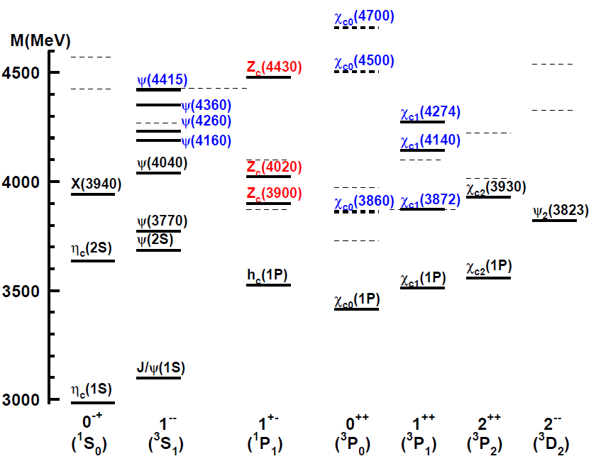
Figure 2: (Color online) The charmonium states. See also caption of Fig. 1. Candidate states are shown by a dashed line. Non-established states with isospin 1 are not shown, see Table 6 for a full list. The $X(4020)$ is shown as $Z_{c}(4020)$. The thresholds for $S$-wave decays into a $c\bar{n}-n\bar{c}$ and $c\bar{s}-s\bar{c}$ in each partial wave are depicted as thin dashed lines. $X(3940)$ is assumed to have pseudoscalar quantum numbers and is interpreted as $\eta_{c}(3S)$.

Table 2: The spectrum of charmonium states below the $D\bar{D}$ threshold.

State	$m$ (MeV)	$\Gamma$ (MeV)	$I^{G}(J^{PC})$
$\psi(1S)$	$3096.900\pm 0.006$	$0.0929\pm 0.0028$	$0^{+}(1^{--})$
$\chi_{c0}(1P)$	$3414.71\pm 0.30$	$10.8\pm 0.6$	$0^{+}(0^{++})$
$\chi_{c1}(1P)$	$3510.67\pm 0.05$	$0.84\pm 0.04$	$0^{+}(1^{++})$
$h_{c}(1P)$	$3525.45\pm 0.15$	$0.70\pm 0.40$	$0^{+}(1^{+-})$
$\chi_{c2}(1P)$	$3556.17\pm 0.07$	$1.97\pm 0.09$	$0^{+}(2^{++})$
$\eta_{c}(2S)$	$3637\pm 4$	14$\pm$7	$0^{+}(0^{-+})$
$\psi(2S)$	$3686.097\pm 0.025$	$0.294\pm 8$	$0^{+}(1^{--})$

Figure 2 shows the charmonium states listed by the PDG Tanabashi:2018oca which contain a $c\bar{c}$ pair in their wave function. States up to $\psi(2S)$ have masses below the open charm ($D\bar{D}$) threshold and are narrow, mostly with a width of a few MeV or even smaller. All expected charmonium states below the $D\bar{D}$ threshold are known and unambiguously established. They are collected in Table 2. The center-of-gravity rule, Eq. (1), holds true for $Q=c,n=1$ with $\delta M=0.08\pm 0.61$ MeV.

Table 3: Thresholds for production two charmed mesons. The quantum numbers correspond to $S$-wave decays.

$J^{PC}$	$0^{-+}$	$1^{--}$	$1^{+-}$	$0^{++}$	$1^{++}$	$2^{++}$	$2^{--}$
	$D_{1}\bar{D}^{*}$	$D_{1}\bar{D}$	$D^{*}\bar{D}$	$D\bar{D}$	$D^{*}\bar{D}$	$D^{*}\bar{D}^{*}$	$D_{2}^{*}\bar{D}$
	4.4228	4.286	3.872	3.730	3.872	4.014	4.326
	$D_{s1}\bar{D}_{s}^{*}$	$D_{s1}\bar{D}_{s}$	$D_{s}^{*}\bar{D}_{s}$	$D_{s}\bar{D}_{s}$	$D_{s}^{*}\bar{D}_{s}$	$D_{s}^{*}\bar{D}_{s}^{*}$	$D_{2s}\bar{D}_{s}$
	4.572	4.428	4.081	3.972	4.081	4.224	4.537

The states above the open charm threshold are significantly broader. Here, two thresholds become important: The threshold for $S$-wave decays into a $c\bar{n}$-$n\bar{c}$ pair – where we include couplings to the ground state $D$ mesons and the narrow even-parity $D$-mesons – and into $c\bar{s}$-$s\bar{c}$ are shown in Table 3. The full charmonium spectrum is displayed in Fig. 2, where the thresholds are shown as dashed lines.

The PDG lists ten $\psi$ states but Fig. 2 shows only eight: There is the well known $\psi(4260)$, seen in the $J/\psi\pi\pi$ Ablikim:2016qzw , $J/\psi K\bar{K}$ Ablikim:2018epj and $\pi^{+}D^{0}D^{*-}$ Ablikim:2018vxx final states, and the candidate state $\psi(4230)$ observed to decay into $\pi\pi h_{c}$ BESIII:2016adj , $\omega\chi_{co}$ Ablikim:2014qwy , and $\pi\pi\psi(2S)$ Ablikim:2017oaf . We assume here that these phenomena are related and correspond to one particle in line with the analysis of Ref. Cleven:2013mka ; Cleven:2016qbn ; this finds further support in the fact that the most recent data for $e^{+}e^{-}\to J\psi\pi^{+}\pi^{-}$ Ablikim:2016qzw clearly peak between $4220$ and $4230$. Likewise, we identify $\psi(4390)$, seen in $\pi\pi h_{c}$ BESIII:2016adj , and $\psi(4360)$ decaying into $\psi(2S)\pi\pi$ Ablikim:2017oaf . The four resonance claims, combined here to two states, are collected in Table 4.

Table 4: BESIII masses and widths (in MeV) of $\psi$ resonances in the mass range from $\psi(4160)$ to $\psi(4415)$. $\psi(4260)$ and $\psi(4360)$ are considered to be established by the PDG, $\psi(4230)$ and $\psi(4390)$ not.

PDG	Mass	Width	Decay	Ref.
$\psi(4230)$	4218.4${}_{-4.5}^{+5.5}$$\pm$0.9	66.0${}_{-8.3}^{+12.3}$$\pm$0.4	$\pi^{+}\pi^{-}h_{c}(1P)$	BESIII:2016adj
	4230$\pm$8$\pm$6	38$\pm$12$\pm$2	$\omega\chi_{c0}(1P)$	Ablikim:2014qwy
	4209.5$\pm$7.4$\pm$1.4	80.1$\pm$24.6$\pm$2.9	$\pi^{+}\pi^{-}\psi(2S)$	Ablikim:2017oaf
$\psi(4260)$	4222.0$\pm$3.1$\pm$1.4	44.1$\pm$4.3$\pm$2.0	$\pi^{+}\pi^{-}J/\psi$	Ablikim:2016qzw
	4228.6$\pm$4.1$\pm$5.9	77.1$\pm$6.8$\pm$6.9	$\pi^{+}D^{0}D^{*-}$	Ablikim:2018vxx
$\psi(4360)$	4320.0$\pm$10.4$\pm$7.0	101.4${}_{-19.7}^{+25.3}$$\pm$10.2	$\pi^{+}\pi^{-}J/\psi$	Ablikim:2016qzw
$\psi(4390)$	4391.5${}_{-6.8}^{+6.3}$$\pm$1.0	139.5${}_{-20.6}^{+16.2}$$\pm$0.6	$\pi^{+}\pi^{-}h_{c}(1P)$	BESIII:2016adj
	4383.8$\pm$4.2$\pm$0.8	84.2$\pm$12.5$\pm$2.1	$\pi^{+}\pi^{-}\psi(2S)$	Ablikim:2017oaf

The Belle collaboration reported a few charmonium states observed in a process in which two $c\bar{c}$ pairs are produced in two-photon collisions Abe:2007jna . Three states are identified with known states: $\eta_{c}(1S)$, a weaker $\chi_{c0}(1P)$ decaying into $D\bar{D}$, and $\eta_{c}(2S)$. Two further states are seen, $X(3940)$ decaying to $D^{*}\bar{D}$, and $X(4160)$ decaying into $D^{*}\bar{D}^{*}$. Tentatively, we assign the $X(3940)$ state to $\eta_{c}(3S)$. If this state were indeed a $0^{-+}$ state, this assignment would in fact be consistent with all views discussed in this paper, since the lowest lying $S$–wave threshold with these quantum numbers is at 4.423 MeV ($cf$. Table 3).

The Belle collaboration reported the observation of a scalar charmonium state in the reaction $e^{+}e^{-}\to J/\psi D\bar{D}$ Chilikin:2017evr . Its mass was determined to $(3862^{+26}_{-32}$${}^{+40}_{-13})$ MeV and its width to $(201^{+154}_{-67}$${}^{+88}_{-82})$ MeV. It is listed as $\chi_{c0}(3860)$ but not included in the PDG summary.

Table 5: Measurements on $X(3915)$ and $\chi_{c2}(3930)$

	Reaction	Mass	Width	$\Gamma_{f}\cdot\Gamma_{i}/\Gamma_{\rm tot}$
$X(3915)$	$\gamma\gamma\to\omega J/\psi$	$3918.4\pm 1.9$	$20\pm 5$	$\ 54\pm\ 9$ eV
$\chi_{c2}(3930)$	$\gamma\gamma\to D\bar{D}$	$3927.2\pm 2.6$	$24\pm 6$	$210\pm 40$ eV

Table 6: Charmonium states with isospin $I=1$ and the discovery reaction and decay. Close-by thresholds are given with the corresponding partial wave. Yes/no indicates if a state is considered to be established or not by the PDG.

	$I^{G}(J^{PC})$	Mass (MeV)	Width (MeV)	Production	Main decay	Threshold	Wave	Establ.	Ref.
$Z_{c}(3900)$	$1^{+}(1^{+-})$	$3918.4\pm 1.9$	$20\pm 5$	$e^{+}e^{-}$ at 4.26 GeV	$\pi\,J/\psi$	$\bar{D}D^{*}$	S	yes	Tanabashi:2018oca
$X(4020)^{\pm}$	$1^{+}(?^{?-})$	$4024.1\pm 1.9$	$13\pm 5$	$e^{+}e^{-}$ at 3.9-4.42 GeV	$\pi^{\pm}h_{c}$a	$\bar{D}^{*}D^{*}$	S	yes	Tanabashi:2018oca
$X(4050)^{\pm}$	$1^{-}(?^{?+})$	$4051^{+24}_{-40}$	$82^{+50}_{-28}$	$\bar{B}^{0}\to K^{-}X^{+}$	$\pi^{\pm}\chi_{c1}(1P)$b	$\bar{D}_{s}D^{*}_{s}$	P	no	Tanabashi:2018oca
$X(4055)^{\pm}$	$1^{+}(?^{?-})$	$4054\pm 3.2$	$45\pm 13$	$\psi(4260)\to\pi X$	$\pi^{\pm}\psi(2S)$	$\bar{D}_{s}D^{*}_{s}$	S	no	Tanabashi:2018oca
$X(4100)^{-}$	$1^{+}/1^{-}$	$4096\pm 20^{+18}_{-22}$	$152\pm 58^{+60}_{-35}$	$B^{0}\eta_{c}\to K^{+}\pi^{-}$	$X\to\pi^{-}\eta_{c}$			$3\sigma$ effect	Aaij:2018bla
$Z_{c}(4200)$	$1^{+}(1^{+-})$	$4196^{+35}_{-32}$	$370^{+100}_{-150}$	$\bar{B}^{0}\to K^{-}X^{+}$	$\pi\,J/\psi$	$\bar{D}_{s}^{*}D_{s}^{*}$	P	no	Tanabashi:2018oca
$R_{c0}(4240)$	$1^{+}(0^{--})^{c}$	$4239^{+50}_{-21}$	$220^{+120}_{-90}$	$\bar{B}^{0}\to K^{-}X^{+}$	$\pi^{\pm}\psi(2S)$	$\bar{D}_{s}^{*}D^{*}_{s}$	P	no	Tanabashi:2018oca
$X(4250)^{\pm}$	$1^{-}(?^{?+})$	$4248^{+190}_{-50}$	$177^{+320}_{-70}$	$\bar{B}^{0}\to K^{-}X^{+}$	$\pi^{\pm}\chi_{c1}(1P)$b	$\bar{D}_{1}D^{*}$	S	no	Tanabashi:2018oca
$Z_{c}(4430)$	$1^{+}(1^{+-})$	$4478^{+15}_{-18}$	$181\pm 31$	$\bar{B}^{0}\to K^{-}X^{+}$	$\pi\,\psi(2S)$	$\bar{D}_{s1}D_{s}$	P	yes	Tanabashi:2018oca

^a Seen in all three charge states.   ^b Seen in Mizuk:2008me , not seen in Lees:2011ik
^c The exotic $0^{--}$ quantum numbers are favored over $1^{+-}$ by one $\sigma$

The PDG identifies the state located near 3930 MeV as $\chi_{c2}(2P)$ state. It is observed in two-photon collisions Lees:2012xs and in $B$ decays delAmoSanchez:2010jr in its decay into $\omega J/\psi$. Very close-by is the $X(3915)$ which was formerly identified with $\chi_{c0}(2P)$ since the analysis favored $J^{PC}=0^{++}$. Table 5 collects the relevant information on $X(3915)$ and $\chi_{c2}(3930)$. In Ref. Zhou:2015uva it was shown, however, that $X(3915)$ may also have $J^{PC}=2^{++}$ quantum numbers when the helicity-2 dominance assumed by BABAR is no longer imposed. Thus, the two states may be one single $\chi_{c2}(2P)$ state with a large molecular component (although current data seems to be compatible with this assignment only if there are large violations of spin symmetry Baru:2017fgv ). Assuming that there is one state only, we evaluate the ratio of branching fractions

$$\frac{{\cal B}\chi_{c2}(2P)\to\omega J/\psi}{{\cal B}\chi_{c2}(2P)\to D\bar{D}} = 0.26\pm 0.07$$ (2)

The OZI-rule-violating decay into $\omega J/\psi$ is seen with a large branching ratio. The threshold for the first $S$-wave decay into open charm, into $D^{*}\bar{D}^{*}$, is with 4014 MeV quite far away.

The $\chi_{c1}(3872)$ has unconventional properties. Its mass of $3871.69\pm 0.17$ MeV coincides exactly at the sum of the $\bar{D}^{0}$ and $D^{*0}$ masses ($3871.68\pm 0.07$ MeV) and falls below the sum of the $D^{-}$ and $D^{*+}$ masses ($3879.91\pm 0.07$ MeV). Hence it decays into $\bar{D}^{0}D^{*0}$ but not into $D^{-}D^{*+}$. Its branching ratio for $\gamma\psi(2S)$ is with $4\%$ significantly larger than its branching ratio for $\gamma J/\psi$ which is well below $1\%$. Its probably most striking feature is, however, that it decays almost equally often into the isovector final state $J/\psi\pi^{+}\pi^{-}$ and into the isoscalar $J/\psi\omega$ final state delAmoSanchez:2010jr , with

$$\frac{{\cal B}\chi_{c1}(3872)\to\omega J/\psi}{{\cal B}\chi_{c1}(3872)\to\pi^{+}\pi^{-}J/\psi} = 0.8\pm 0.3.$$ (3)

Table 7: Masses, widths (in MeV) and quantum numbers of $\phi J/\psi$ resonances from Ref. Aaij:2016iza and possible spectroscopic interpretations.

	$\chi_{c1}(4140)$	$\chi_{c1}(4274)$	$\chi_{c0}(4500)$	$\chi_{c0}(4700)$
Mass	$4146.5$	$4273.3$	$4506$	$4704$
$\sigma_{\rm stat},\sigma_{\rm syst}$	$\pm$$4.5^{+4.6}_{-2.8}$	$\pm$$8.3^{+17.2}_{-\ 3.6}$	$\pm$$11^{+12}_{-15}$	$\pm$$10^{+14}_{-24}$
Width	$83$	$56$	$92$	$120$
$\sigma_{\rm stat},\sigma_{\rm syst}$	$\pm$$21^{+21}_{-14}$	$\pm$$11^{+\ 8}_{-11}$	$\pm$$21^{+21}_{-20}$	$\pm$$31^{+42}_{-33}$
	$\chi_{c1}(3P)$	$\chi_{c1}(4P)$	$\chi_{c0}(5P)$	$\chi_{c0}(6P)$

Above this mass, two further $1^{++}$ states were reported, $\chi_{c1}(4140)$ and $\chi_{c1}(4274)$. Both are seen in $B^{\pm}\to J/\psi\phi K^{\pm}$ decays, the former state by several collaborations Chatrchyan:2013dma ; Abazov:2013xda ; Lees:2014lra ; Aaltonen:2011at ; Aaij:2016iza (only the latest reference of the collaborations are given here), the latter one by CDF Aaltonen:2011at and LHCb Aaij:2016iza .

The LHCb paper Aaij:2016iza is based on the largest data sample. The amplitude analysis of the reaction $B^{+}\to K^{+}\phi J/\psi$ and $\phi\to K^{+}K^{-}$ included the known excited kaon and four $\omega J/\psi$ resonances. The two lower-mass $\omega J/\psi$ resonances gave the best fit for $J^{PC}=1^{++}$, the two at higher masses were found to have $J^{PC}=0^{++}$. The results are listed in Table 7. The two scalar states are not listed in the PDG summary list.

Isovector states with decay products having hidden charm like $J/\psi$ or $h_{c}$ and/or open charm can obviously not have a pure $c\bar{c}$ component in their wave function as they carry exotic quantum numbers. The observations are listed in Table 6. Three of these states are accepted by the PDG. Two of them are $1^{+-}$ states and are therefore called $Z_{c}({\rm mass})$. Most probably, the third accepted state, $X(4020)$ with $I^{G}=1^{+}$ has also $J^{PC}=1^{+-}$ quantum numbers.

One state – seen in its $\pi\psi(2S)$ decay – is called $R_{c0}(4240)$. Its quantum numbers $1^{+}(0^{--})$ are preferred over $1^{+}(1^{+-})$ by one standard deviation. This is presumably insufficient to claim a new resonance, and we combine this observation with $Z_{c}(4200)$. Masses and widths are compatible with this identification. In the following section we discuss the implications of their existence from the three different points of view introduced above.

IV Discussion

In this section we now discuss the three views introduced in the introduction in the light of the mentioned experimental observations.

IV.1 Consequences of View I

In this view all states near and above the first heavy open flavor $S$-wave threshold with matching quantum numbers are classified as molecular states. We begin the discussion with the charged states. The lowest lying charged states have $J^{PC}=1^{+-}$ ($Z_{c}(3900)$, $Z_{c}(4020)$, $Z_{b}(10610)$ and $Z_{b}(10650)$) and are consistent with being molecules formed by a pseudoscalar and a vector or two vector mesons, respectively. Moreover, each one of them is located very close to one of the four thresholds, $D\bar{D}^{*}$, $D^{*}\bar{D}^{*}$, $B\bar{B}^{*}$, $B^{*}\bar{B}^{*}$. A problem occurs with $Z_{c}(4430)$: This state has the same $J^{PC}$ as the ones mention, however, it is well above the lowest $S$–wave threshold. Thus, within View I the only possible explanations for the $Z_{c}(4430)$ are that it is either a kinematic effect, as proposed in Ref. Pakhlov:2014qva , or a $P$–wave molecular state composed of $D_{1}\bar{D}$ as proposed in Ref. He:2017mbh .

Figure 3: (Color online) The $\psi_{c}$ and $\Upsilon$ mass spectra in View I. (Black) filled circles: ${}^{3}S_{1}$ $Q\bar{Q}$ mesons; (blue) x’s: $\psi(nD)$ $Q\bar{Q}$ mesons; (green) y’s: $D$-wave $Q\bar{Q}$ mesons; (red) open circles: extraordinary states. Thresholds for the lowest $S$-wave decays into $B_{1}\bar{B}$ or $D_{1}\bar{D}$ are shown by a pair of small vertical bars.

As soon as we accept that the $Z$–states are of molecular nature, we also expect molecular states to occur in the isoscalar sector. One argument in support of this is e.g. that for the exchange of an isovector particle like the pion or the rho meson between two isospin $1/2$ states one has

$$\langle II_{3}|\tau_{1}\cdot\tau_{2}|II_{3}\rangle=\left\{{\phantom{-}1\mbox{ for }I=1}\atop{-3\mbox{ for }I=0}\right.\ .$$ (4)

In addition, when the $C$ parity gets switched the central part of the potential acquires an additional sign. Thus, if isovector exchanges contribute to a relevant amount to the binding of the $Z$–states with $I=1$ and $J^{PC}=1^{+-}$, then one should expect that they also generate isoscalar bound states with $J^{PC}=1^{++}$, since the resulting interaction is attractive in both channels and it is even a factor 3 stronger in the isoscalar one — in this sense $Z_{c}(3900)$ and $\chi_{c1}(3872)$ would be very close relatives. Accordingly, it should be possible to produce both with an analogous mechanism. This observation was employed in Ref. Guo:2013nza to predict that $\chi_{c1}(3872)$ must be copiously produced in $e^{+}e^{-}\to\gamma\chi_{c1}(3872)$ given that $Z_{c}(3900)$ was found in $e^{+}e^{-}\to Z_{c}(3900)\pi$ — a prediction confirmed experimentally at BESIII Ablikim:2013dyn — these transitions might well be favored also by a possible molecular structure of the source state for the transition, $\psi(4260)$, (see discussion below) Wang:2013cya and by some kinematical enhancement Wang:2013hga . . However, there should not be an isoscalar $1^{++}$ state near the $D^{*}\bar{D}^{*}$ threshold as a relative of the $Z_{c}(4020)$, since $D^{*}\bar{D}^{*}$ in spin 1 $S$-wave has a negative $C$–parity. Moreover, $if$ single isovector exchanges, like one-pion exchange, provide the most important contribution to the binding of the $Z$–states via the central potential (that drives the $S$ wave to $S$ wave transitions), there should not be any isoscalar bound states with $J^{PC}=1^{+-}$ or isovector ones with $J^{PC}=1^{++}$ with the same constituents. This is a non-trivial prediction from the molecular picture. It relies on the additional assumption that single isovector meson exchanges provide an essential part of the scattering potential that eventually leads to the generation of the molecular states. Up to date this prediction is in line with observation, however, the recent analysis of Ref. Wang:2018jlv revealed that the most important contribution of the one pion exchange contribution comes from the $S-D$ transition driven by the tensor force. Since this piece enters quadratically into the binding potential in the $S$–wave, it appears to provide attraction in all channels and the argument presented above should be refined.

Heavy quark spin symmetry allows one to predict additional states: At leading order heavy quark spin symmetry one can construct two contact terms for the interaction between the two ground state $D$–mesons. Moreover, these contact terms appear in the same linear combination in the $1^{++}$ channel and in the $2^{++}$ channel Guo:2013sya . Accordingly, the $1^{++}$ state $\chi_{c1}(3872)$ located very near the $D\bar{D}^{*}$–threshold should have a spin 2 partner. The latter state, often called $X_{2}(4020)$ or – according to the PDG naming scheme – $\chi_{c2}(4020)$, is located close to the $D^{*}\bar{D}^{*}$ threshold. Once one-pion exchange is included transitions from the $D^{*}\bar{D}^{*}$ $S$-wave with spin 2 to the $D\bar{D}$-$D$-wave become possible which can lead to widths of a few MeV Albaladejo:2015dsa to tenth of MeV Baru:2016iwj .

While the data in the isoscalar states in the charmonium mass range is insufficient to fix the two mentioned contact terms the situation is different for the isovector states. For example the heavy quark spin partners of the $Z_{b}$ states were studied in Refs. Voloshin:2011qa ; Mehen:2011yh ; Guo:2013sya ; Baru:2019xnh .

The interpretation of $\chi_{c1}(3872)$ as $D^{*}\bar{D}$ molecule suggests the existence of a $D_{s}^{*}\bar{D}_{s}$ molecule close to 4.081 GeV. However, the mass of the next heavier state with $J^{PC}=1^{++}$ is $\chi_{c1}(4140)$ at $4146.8\pm 2.4$ MeV. It is thus located about 60 MeV above the mentioned threshold. Thus a $D_{s}^{*}\bar{D}_{s}$ molecular nature of this state is difficult to anticipate in particular since it would then predominantly decay into that channel which should lead to a significantly broader width than the observed 20 MeV. An alternative possibility could be a $D_{s}^{*}\bar{D}_{s}^{*}$ bound state whose threshold is located 80 MeV above the $\chi_{c1}(4140)$. However, so far basically all calculations could get a state in this mass range from $D_{s}^{*}\bar{D}_{s}^{*}$ only with $J^{PC}=0^{++}$ or $2^{++}$ — for a recent summary of the situation we refer to Ref. Wang:2017mrt . In this work the structure called $X(4160)$ in the RPP is claimed to originate from the $D_{s}^{*}\bar{D}_{s}^{*}$ dynamics. As it stands, also the $\chi_{c1}(4274)$ – if confirmed – seems incompatible with View I.

There is an interesting difference between the molecular picture and the predictions of the quark model already for the $D^{(*)}\bar{D}^{(*)}$ systems: While in the quark model there exists for each radial excitation one state with $J^{PC}=1^{+-}$, in the molecular picture there are typically two, since both the $D\bar{D}^{*}$ as well as the $D^{*}\bar{D}^{*}$ channel can couple to these quantum numbers in an $S$–wave. This is the pattern already seen for the charged states, however, so far not in the isoscalar channels.

Besides non–perturbative $D\bar{D}$, $D^{*}\bar{D}$ and $D^{*}\bar{D}^{*}$ interactions, also non–perturbative interactions between $D_{1}$ or $D_{2}^{*}$ and $\bar{D}$ or $\bar{D}^{*}$ mesons can lead to hadronic molecular states. Since the $(D_{1},D_{2}^{*})$ spin multiplet carries even parity, those will have odd parity for $S$–wave interactions. In View I one is thus obliged to interpret the $1^{--}$ states $\psi(4260)$ aka $Y(4260)$, $\psi(4360)$ aka $Y(4360)$ as well as $\psi(4415)$ as $D_{1}\bar{D}$, $D_{1}\bar{D}^{*}$ and $D_{2}^{*}D^{*}$ molecular states, respectively Wang:2013cya ; Cleven:2015era ; Wang:2013kra . This nicely explains why negative parity exotic candidates are about 400 MeV heavier that their even parity partners: This mass difference reflects the $D_{1}(2420)$–$D^{*}$ mass difference. Accordingly, the molecular picture predicts that exotic pseudoscalars should be even heavier, since the quantum numbers $0^{-+}$ can only be reached in an $S$-wave with the constituents $D_{1}\bar{D}^{*}$, with a threshold yet another 140 MeV higher Cleven:2015era . Moreover, one expects a clear signal of $Y(4260)$ in the $D\bar{D}^{*}\pi$ final state since $D^{*}\pi$ is the main decay channel of the $D_{1}$. This signal was predicted in Ref. Cleven:2013mka and confirmed recently at BESIII Ablikim:2018vxx .

For the vector states, view I is summarized in Fig. 3. The $Q\bar{Q}$ mesons are represented by (black) filled circles or, for states assigned to $D$-waves, by (green) crosses, the extraordinary states by (red) open circles. The thresholds for the lowest $S$-wave decays into $B_{1}\bar{B}$ or $D_{1}\bar{D}$ are shown by a pair of small vertical bars. One state below this threshold and all states above are classified as extraordinary states. In this view the $\psi(4660)$ aka $Y(4660)$ is to be seen as $\psi(2S)f_{0}(980)$ molecular state Abe:2007jna , since it is located right at the corresponding threshold. A non-trivial prediction that emerges from this assignment is the existence of a spin partner of the $Y(4660)$ — a bound state of $\eta_{c}(2S)$ and $f_{0}(980)$ Guo:2009id .

Unfortunately within a hadronic effective field theory it is not possible to make the relation between the molecular structures in the bottomonium sector and those in the charmonium sector quantitative Baru:2018qkb . It therefore appears not possible to predict the spectrum of exotic bottomonia from the rich spectrum of charmonia.

A very interesting aspect that comes with the molecular assignment is the role of the heavy quark spin in decays: In the heavy quark limit the spin of the heavy quark decouples from the system. In addition, in $e^{+}e^{-}$ collisions that lead to final states which contain a heavy quark and its antiquark, the heavy quark-antiquark pair is produced directly at the photon vertex in spin 1 to avoid the need to generate heavy quarks via gluonic interactions — a process suppressed as a result of asymptotic freedom. Accordingly one would expect to see in reactions like $e^{+}e^{-}\to(\bar{Q}Q)2\pi$ the $\bar{Q}Q$ pair by far predominantly in a spin one state. For the low lying heavy quarkonia this is indeed the case — for example the branching ratio $\Upsilon(3S)\to\Upsilon(2S)\pi^{+}\pi^{-}$ is with 4.4% more than two orders of magnitude larger than the upper bound for $\Upsilon(3S)\to h_{b}(1P)\pi^{+}\pi^{-}$ currently quoted as $1.2\times 10^{-4}$. In contrast to this the $Z_{b}$ states decay equally often into spin 1 and spin 0 final states. This pattern finds a natural explanation in the molecular picture where  Bondar:2011ev

$$Z_{b}(10610)\sim B^{*}\bar{B}-B\bar{B}^{*}=\frac{1}{\sqrt{2}}\left(0^{-}_{\bar{q}q}\otimes 1^{-}_{\bar{b}b}-1^{-}_{\bar{q}q}\otimes 0^{-}_{\bar{b}b}\right),$$

$$Z_{b}(10650)\sim\quad\leavevmode\nobreak\ B^{*}\bar{B}^{*}\quad\leavevmode\nobreak\ =\frac{1}{\sqrt{2}}\left(0^{-}_{\bar{q}q}\otimes 1^{-}_{\bar{b}b}+1^{-}_{\bar{q}q}\otimes 0^{-}_{\bar{b}b}\right).$$ (5)

The $Z_{b}$ states were observed in the decays of $\Upsilon(10860)$ which is far way from an $S$–wave threshold with matching quantum numbers. Interestingly the data in the $h_{b}\pi$ final states accordingly are non-vanishing only near the $Z_{b}$ peaks, for apparently in this case the $Z_{b}$ intermediate states are necessary to populate the final state with heavy quark spin equal to 0. This picture is supported by the fact that in the related $\Upsilon(nS)\pi$ spectra there is a lot of strength even outside the $Z_{b}$ peaks. The situation is very much different in case of the decays of $Y(4260)$: While this state is also seen in both $h_{c}\pi\pi$ and $J/\psi\pi\pi$ final states with similar strength, here even in the data with an $h_{c}$ in the final state there is a lot of strength observed also outside the $Z_{c}$ peaks. This could be interpreted as an indication of a $D_{1}\bar{D}$ molecular nature of the $Y(4260)$, since Li:2013yka

$$(D_{1}\bar{D}-\bar{D}_{1}D)\sim\frac{1}{2\sqrt{2}}\psi_{11}+\frac{\sqrt{5}}{2\sqrt{2}}\psi_{12}+\frac{1}{2}\psi_{01},$$ (6)

where $\psi_{1J}=1_{H}^{--}\otimes J_{L}^{++}$ and $\psi_{01}=0_{H}^{-+}\otimes 1_{L}^{+-}$ where $H$ and $L$ stand for the heavy and light quark-antiquark pair. The analogous argument applies for $Y(4360)$. The presence of light quarks in the wave function for $Y(4260)$ finds further support in the analysis of Ref. Chen:2019mgp .

IV.2 Consequences of View II

We start the discussion of View II with $\chi_{c1}(3872)$ aka $X(3872)$. In this view, this state is identified with $\chi_{c1}(2P)$. The view does not deny that $X(3872)$ has a large $D^{*}\bar{D}$ component: its mass happens to be close to the sum of the $D^{*0}$ and $\bar{D}^{0}$ masses and is synchronized to match the exact mass Bugg:2008wu . The $c\bar{c}$ pair creates a $d\bar{d}$ pair thus dressing the $c\bar{c}$ core with a $D^{*0}\bar{D}^{0}$ cloud. The pole leads to a strong $S$-wave attraction between the $D^{*0}$ and $\bar{D}^{0}$ mesons. However, only one resonance is formed.

One might think that a hard $c\bar{c}$ core of $\chi_{c1}(3872)$ is needed to explain its copious production in hard processes in $\bar{p}p$ collisions at $\sqrt{s}$=1.96 TeV Acosta:2003zx and at 7 TeV Aaij:2011sn . This reasoning is put forward in Refs. Bignamini:2009sk ; Bignamini:2009fn ; Esposito:2015fsa ; Esposito:2017qef but was criticised in Refs. Artoisenet:2009wk ; Artoisenet:2010uu ; Albaladejo:2017blx ; Guo:2014sca ; Guo:2014ppa ; Braaten:2018eov . At this point in time it is fair to say that there is no consenus in the literature wether or not large momentum transfer reactions can act as a filter to states with quark–anti-quark cores.

Using QCD sum rules to calculate the width of the radiative decay of the $\chi_{c1}(3872)$ meson, the authors of Ref. Matheus:2009vq ; Nielsen:2010ij conclude that the X(3872) is approximately 97% a charmonium state with a 3% admixture of $D^{0}D^{*0}$ molecule ($\sim 88$%) and a $D^{+}D^{*-}$ molecule ($\sim 12$%). This result is basically reproduced in Ref. Zanetti:2011ju ; the authors discuss the intrinsic uncertainties in their calculations and underline that the $c\bar{c}$ part of the state plays a very important role in the determination of branching ratios. The authors of Ref. Meng:2014ota study the $B\to KD\bar{D}^{*}$ and $B\to KJ/\psi\pi^{+}\pi^{-}$ decay processes and claim that $X(3872)$ is mainly a $c\bar{c}$ resonance with a small contribution generated by $\bar{D}D^{*}$ final state interaction. In Zhou:2017dwj ; Zhou:2017txt , the $\chi_{c1}(3872)$ is estimated to have a strong molecular and a 10-30% $c\bar{c}$ component. From a study of radiative decays, the authors of Ref. Cincioglu:2019gzd conclude that a wide range of $c\bar{c}$ versus molecular components is consistent with the data. However, in Ref. Guo:2014taa it is pointed out that it is impossible to quantify the impact of the short-range contributions in an effective field theory based on hadrons and radiative decays of the $\chi_{c1}(3872)$ are sensitive to this part of the wave function. The radiative decays can hence not be used as an argument disfavoring the molecular view but the molecular view can – based on the same argument – not rule out a significant $Q\bar{Q}$ core.

The next state with $J^{PC}=1^{++}$ above $\chi_{c1}(3872)$ is $\chi_{c1}(4140)$ which is seen only in its decay into $J/\psi\phi$. In View II, it is interpreted as $\chi_{c1}(3P)$, followed by $\chi_{c1}(4274)$ as $\chi_{c1}(4P)$. In View I, $\chi_{c1}(4274)$ can possibly be understood as a bound state of $D_{s}^{*}\bar{D}_{s}^{*}$ Branz:2009yt . In View II, it has a $c\bar{c}$ core but could be dressed by a $D_{s}^{*}\bar{D}_{s}$ cloud.

View II identifies the $\chi_{c2}(3930)$ state with $\chi_{c2}(2P)$. Likewise, the $\chi_{c0}(3860)$ candidate is interpreted as $\chi_{c0}(2P)$ state. Both resonances fall just in between important thresholds at 3730, 3972 and 4014 MeV.

Figure 4: The $\psi_{c}$ and $\Upsilon$ mass spectra in View II. The $\psi(3770)$ and $\psi(4160)$ are interpreted as $\psi(1D)$ and $\psi(2D)$ and marked by (blue) x’s, the two states with $J^{PC}=2^{--}$ by (green) y’s. The $\psi(4040)$ and $\psi(4415)$ states are interpreted as $\psi(3S)$ and $\psi(4S)$. The $\psi(4260)$ and $\psi(4360)$, mostly interpreted as unconventional states, are suggested to be generated by an interplay of interference effects and threshold singularities. At this stage the $\Upsilon(11020)$ does not fit into the scheme. Note that the PDG mass values sometimes differ significantly from the mass given in the name of a state.

Figure 5: The $\psi_{c}$ and $\Upsilon$ mass spectra. The $\psi(4040)$, $\psi(4260)$, and $\psi(4415)$ have masses which suggest that there should be identified with $\psi(3S)$ to $\psi(5S)$, they are marked by filled circles. The $\psi(4160)$ and $\psi(4360)$ are marked with (blue) x’s and identified with $\psi(2D)$ and $\psi(3D)$. $J^{PC}=2^{--}$ states are shown by (green) y’s. The identification of $\psi(4660)$ and $\Upsilon(11020)$ is open.

If $X(3872)$ can be identified with $\chi_{c1}(2P)$, we can apply the center-of-gravity rule to predict the mass of the $h_{c}(2P)$. The center-of-gravity rule of Eq. (1) proved to be well satisfied for $b\bar{b}$ mesons in the $1P$ and $2P$ level and for $c\bar{c}(1P)$ mesons. In Ref. Lebed:2017yme it is argued that the center-of-gravity rule of Eq. (1) can be used as a diagnostic for $\bar{Q}Q$ states. Since only three states in the $2P$ level are known, $\chi_{c2}(3930)$, $\chi_{c1}(3872)$, $\chi_{c0}(3860)$, we can use Eq. (1) only to predict the $h_{c}(2P)$ mass and find

$$M_{h_{c}(2P)} = (3900\pm 10){\rm\,MeV.}$$ (7)

In View II, we thus require the existence of one and only one $1^{+-}$ state at a mass of about 3900 MeV. This is in line with Ref. Zhou:2017dwj ; Zhou:2017txt : The authors identify $\chi_{c0}(3862)$, $\chi_{c1}(3872)$, and $\chi_{c2}(3930)$ with the $\chi_{c}(2P)$ states and calculate the $h_{c}(2P)$ mass to 3902 MeV.

This is clearly a different prediction compared to what emerges in the molecular picture of View I, where, as mentioned above, two $1^{+-}$ can (but don’t need to) emerge, one near to the $D\bar{D}^{*}$ threshold (and thus close to 3900 MeV) and one close to the $D^{*}\bar{D}^{*}$ threshold at 4020  MeV.

Mass, production and decay modes of $X(3940)$ are compatible with an assignment to $\eta_{c}(3S)$ but its quantum numbers have not yet been determined. As a pseudoscalar state, it is compatible with View I and View II, since the lowest relevant threshold is much higher than 3940 MeV.

Now we turn to the vector states. Figures 5 and 5 compare the spectrum of $\Upsilon$ states with that of $\psi$ states in two different realisations of View II. First we discuss their common features.

$\Upsilon(2S)$ has a mass 563 MeV above $\Upsilon(1S)$, $\psi(2S)$ is found 589 MeV above $J/\psi$. $\Upsilon(3S)$ is situated 331.5 MeV above $\Upsilon(2S)$. We thus expect the $\psi(3S)$ state just above 4035 MeV. Indeed, a $\psi(4040)$ exists. In the quark model, we interpret this state, due to its mass and decay modes, as $\psi(3S)$. The quantum numbers $I^{G}(J^{PC})=0^{-}(2^{--})$ were suggested for $\psi_{2}(3823)$ and $\Upsilon_{2}(1D)$, but both need confirmation. If confirmed they seem to be related and $\psi_{2}(3823)$ is likely $\psi_{2}(1D)$. The $\psi(3770)$ state is close in mass to $\psi_{2}(3883)$; in the quark model it can be assigned to the $\psi(1D)$ state, likely with some mixing with $\psi(2S)$. Above this mass, the two scenarios differ. The first scenario assumes that $\psi(4260)$ and $\psi(4360)$ are not real resonances, the second scenario assigns the two resonances to the series of $\psi(nS)$ and $\psi(nD)$ resonances. In both scenarios $\psi(4415)$ is assigned to the $\psi(nS)$ series and interpreted as $\psi(4S)$ in the first, as $\psi(5S)$ in the second scenario.

First scenario: $\Upsilon(4S)$ is situated 224 MeV above $\Upsilon(3S)$. We may thus expect $\psi(4S)$ at about 4300 MeV. There are claims for four states close in mass, see Table 4. Their masses could be acceptable, however, as states with a large $Q\bar{Q}$ component at the origin, one may expect that their $e^{+}e^{-}$ decay width should be larger; the decay modes of these states are completely unexpected. Possibly, none of them is the $\psi(4S)$. Hence we first try to identify $\psi(4415)$ with $\psi(4S)$.

Table 8 collects some results on vector charmonium states. In an R scan above $\psi(2S)$, the BES collaboration observed four further states, $\psi(3770)$, $\psi(4040)$, $\psi(4160)$, $\psi(4415)$ Ablikim:2007gd . While $\psi(3770)$ decays predominantly into $D\bar{D}$, the other mesons, including $\psi(4260)$ and $\psi(4360)$, have a large number of decay options. However, none of them listed by the PDG with a finite branching ratio, except of the (10$\pm$4)% for the $\psi(4415)\to D_{2}^{*}\bar{D}$ decay Pakhlova:2007fq . Apart from the “stable” $J/\psi$ and $\psi(2S)$, the total widths of these states have a similar magnitude. The $e^{+}e^{-}$ partial decay widths decrease steadily for the states assigned in Table 8 to the $nS$ series; states assigned to the $nD$ series have somewhat smaller $e^{+}e^{-}$ partial decay widths: The density of the wave function near the origin decreases with $n$ and is smaller for $D$-wave states. The relatively large value for $\psi(4160)$ may indicate a significant $3S$ contribution.

Table 8: Charmonium states with $J^{PC}=1^{--}$ in the first scenario of View II.

State	$\Gamma_{\rm tot}$			$\Gamma_{e^{+}e^{-}}$		Assigned
$J/\psi$	$0.0929$$\pm 0.0028$	MeV		5547	eV	$\psi(1S)$
$\psi(2S)$	$0.294$$\pm$$0.008$	MeV		2331	eV	$\psi(2S)$
$\psi(3770)$	$87.04$$\pm$$0.35$	MeV		261	eV	$\psi(1D)$
$\psi(4040)$	$80\pm 10$	MeV		850	eV	$\psi(3S)$
$\psi(4160)$	$70\pm 10$	MeV		483	eV	$\psi(2D)$
$\psi(4415)$	$62\pm 20$	MeV		580	eV	$\psi(4S)$

The $\psi(4415)$ fits into this series, and based on Table 8, we are tempted to interpret this state as $Q\bar{Q}$. When its mass is compared to $\Upsilon(4S)$, it seems to have too high a mass. On the other hand, its mass is just on the $D_{s1}\bar{D}_{s}$ threshold and close to the $D_{2}\bar{D}^{*}$ threshold. A threshold is known to attract the pole position Bugg:2008wu — the possible impact of the hidden strangeness channel on the $\psi(4415)$ is discussed in Ref. Cao:2017lui . Hence it is not unreasonable to identify $\psi(4415)$ with $\psi(4S)$. Due to its mass at the $D_{s1}\bar{D}_{s}$ threshold it develops a significant molecular component Wang:2013cya ; Cleven:2015era which dominates the decay modes. However, in View II it owes its existence to its $Q\bar{Q}$ core.

There are eight observations of resonances with identical quantum numbers claimed in the mass interval between 4200 and 4400 MeV. Even if we combine five of these observations to two states (see Table 4), the density of states is rather high. The peak cross sections for $\psi(4160)$ and $\psi(4415)$ are about 15.000 pb, with significant interference between the two states Ablikim:2016qzw . The cross section for $e^{+}e^{-}\to\psi(4260)$ and $\psi(4360)\to J/\psi\pi^{+}\pi^{-}$ is with at most 80 pb less than 1% of the cross section for $\psi(4160)$ and $\psi(4415)$. A possible explanation for the structures called $\psi(4260)$ and $\psi(4360)$ within View II could be that the two resonances $\psi(4160)$ and $\psi(4415)$ both have a small coupling to OZI violating final states. In Ref. Chen:2017uof it is shown how interference effects can then lead to the observed structures in the absence of true resonances. The authors of Ref. Chen:2017uof suggest that only $\psi(4220)$ might survive as a resonance. However, the best estimate for the mass of $\psi(4160)$ is 4190 MeV, just 30 MeV lower than the mass of the conjectured $\psi(4220)$. These two observations may hence be one single state.

There is an important caveat: The fits of Ref. Chen:2017uof reveal that the existing data in the $h_{c}\pi\pi$ and $J/\psi\pi\pi$ channels can be described only, if one allows for a huge violation of spin symmetry which appears not to be natural. Moreover, the analysis of Ref. Chen:2017uof introduces a strong non-resonant background, also with large spin symmetry violation and fine tuned in each channel to suppress the true resonance signals at the resonance locations. Nevertheless, the analysis shows that there might be solutions in which the states between $\psi(4160)$ and $\psi(4415)$ are not needed. We remind the reader that there are very significant thresholds between 4100 and 4500 MeV: $S$-wave decays into $D_{1}\bar{D}$ are open at 4286 MeV, into $D_{s1}\bar{D}_{s}$ at 4428 MeV; $P$ wave decays into $D_{s}^{*}\bar{D}_{s}$ open at 4.081 MeV, into $D_{1}\bar{D}^{*}$ at 4228 MeV. A coupled-channel analysis of all final states with proper evaluation of all kind of singularities is missing. Possibly, there is no state at all between $\psi(4190)$ and $\psi(4415)$.

Second scenario: An alternative interpretation of the $\psi$ mass spectrum within the $Q\bar{Q}$ quark model was given in Ref. Klempt:2007cp where the $\psi(4260)$ was interpreted as $\psi(4S)$, the $\psi(4360)$ as $\psi(3D)$ and $\psi(4415)$ as $\psi(5S)$. Figure 5 shows that interpretation. The excitation energies of the low-mass charmonium system are increasingly larger than those in the bottomonium spectrum, while the opposite pattern is observed at higher masses. This looks unnatural. We emphasize, however, that the identification of $\psi(4260)$ with $\psi(4S)$, of $\psi(4360)$ with $\psi(3D)$ and of $\psi(4415)$ with $\psi(5S)$ is an over-simplification. All states can mix: Ref. Wang:2018rjg gives a fit to data assuming that the $4S$ and $3D$ states mix to form $\psi(4260)$ and $\psi(4360)$ and the $5S$ and $4D$ mix to form the $\psi(4415)$ and a hypothetical $\psi(4500)$. Further, all states may contain a molecular component. View II just claims that these states have a $c\bar{c}$ seed and that this seed is decisive for the existence of these states.

The first scenario is approximately compatible with quark-model calculations using the Cornell potential; the second scenario is compatible when a screened potential is used. This is discussed in Section VI.

In quark models with $Q\bar{Q}$ states only, charged heavy-quark states are not admitted. In View II the structures seen in isovector channels are not regular resonances with a pole in the $S$–matrix. The $Z_{c}$ and $Z_{b}$ states would have to be produced via perturbative rescattering in the final state. At present, this possibility is not (yet?) ruled out. A softer version of View II forbids only hidden exotics but allows for states beyond the quark model which cannot be reduced to $Q\bar{Q}$, which means that they have quantum numbers not accessible to $Q\bar{Q}$.

The $\Upsilon(10860)$ could decay into $B^{*}\bar{B}\pi$ where the $B^{*}\bar{B}$ system rescatters into $\Upsilon(nS)\pi$ when $B^{*}$ and $\bar{B}$ are in $S$-wave and have little relative momentum. It was shown in Ref. Guo:2015umn that rescattering can produce a loop in an Argand diagram. In various works, several of the $XYZ$ states are suggested to be only a kinematical enhancement Bugg:2004rk ; Bugg:2011jr ; Chen:2011pv ; Chen:2011xk ; Chen:2011pu ; Chen:2013coa ; Chen:2013wca ; Swanson:2014tra ; Swanson:2015bsa . A newly created $c\bar{c}$ pair has a strong affinity to decay into a pair of (possibly excited) $D$ or $D_{s}$ mesons. There are a few $D/D_{s}$ mesons which are narrow, so that rescattering is possible. The thresholds for the production of a pair of narrow charmed mesons are given in Table 3. The $X(4100)$ has no close-by threshold but it is seen only as effect with three standard deviation significance. Also $Z_{c}(4430)$ has no close-by $S$-wave threshold but is seen as a clear signal. There are two thresholds close to its mass, for $D_{1}\bar{D}^{*}$ and $D_{s1}\bar{D}_{s}$ but in $S$-wave they belong to $0^{-+}$ and $1^{--}$ quantum numbers. Still, as mentioned above, this state could have emerged from a triangle singularity Pakhlov:2014qva .

The authors of Ref. Pilloni:2016obd study possible scenarios for the related $Z_{c}(3900)$ which might be a compact QCD state, a virtual state, or a kinematical enhancement. The authors conclude that current data are not precise enough to distinguish between these hypotheses. In Ref. Guo:2014iya it was demonstrated that in particular the channel that is related to the nearby threshold is sensitive to the presence or the absence of a pole. Thus here, experiment will eventually be able to tell the difference. The reasoning of Ref. Guo:2014iya was questioned in Ref. Swanson:2015bsa . There, however, different physics drives the structures in the near-by channel and the others: Formfactors in the former, cusps in the latter. This is not only unsatisfying, it also leads to the prediction that there should be similar structures near each $S$-wave threshold which does not seem to be the case. But given the controversy in the literature one may conclude that at present there is no forcing evidence that genuine isovector states with a normal pole structure in the complex scattering plane exist.

V Consequences of View III

In the previous sections we have seen that both View I and View II have problems with certain states in the spectrum. Some of those problems might get resolved with the appearance of better data, but some might not. We would therefore like to now confront the current data situation with View III, which allows for the co-existence of molecular states and quark model states. In the literature there are various model calculations that try to capture this view — see, e.g., Ref. Ortega:2019tby and references therein.

To get a physics understanding of how such an interplay of different structures could emerge in QCD we could start from the large $N_{c}$ limit of QCD tHooft:1973alw . In this limit there exist infinite towers of stable $\bar{Q}Q$ states (and eventually also tetraquarks which were added to the discussion in Ref. Weinberg:2013cfa ). As one then starts reducing the number of colors gradually, the coupling of the quark model states to two–meson states grows. Accordingly the states above the two hadron–threshold acquire a finite life time. It was demonstrated in Ref. Hammer:2016prh in a toy model with only one continuum channel included that, as one increases the coupling further, something unusual happens (analogous results were reported earlier in Ref. vanBeveren:2006ua ): While most of the states get stable again and end in the limit of very large couplings again at masses similar to the original ones, typically one state very strongly couples to the continuum channel. The latter kind of state might be viewed as a molecular state while the others preserve their $\bar{Q}Q$ nature, however, with changed decay patterns. The calculations in Ref. Hammer:2016prh were performed for a fixed number of input quark model states, however, the pattern was observed independent of the number of states involved. In particular: the state that showed a very strong coupling to the continuum was a mixture of all other states included regardless of their distance to the actual pole location. Such a collective phenomenon might indicate the onset of significant $t$–channel exchanges for the binding potential — after all quark hadron duality indicates that an infinite sum of $s$–channel poles can be mapped onto an infinite sum of $t$-channel poles. At the end this provides an understanding how it could be possible that there is a coexistence of quark model states and molecular states with nearly no cross talk between the two groups.

View III admits the possibility that $\chi_{c1}(4274)$, $\chi_{c0}(4300)$, $\chi_{c0}(4500)$ could exist as quark model states even in the presence of lower lying molecular structures. Analogously, there could be quark model states in the vector channel above 4.4 GeV even with $Y(4260)$ and $Y(4360)$ being molecular states. At present the $\psi(4415)$ could be both — a $D_{2}\bar{D}^{*}$ molecular state as well as a quark model state or a mixture of both. If indeed there is a mechanism at work as revealed in Ref. Hammer:2016prh , any quark model state that appears above an open $S$–wave threshold should not decay into this channel. Accordingly, one would expect rather narrow quark model states even higher up in the spectrum.

VI Comparison with model calculations

View I suggests that the $Q\bar{Q}$ should be screened; the usual Cornell potential with a Coulomb part proportional to $\alpha_{s}/r$ and a confinement part linearly rising with $r$ should be replaced by a Coulomb potential plus a term that could be modelled by $b(1-e^{-\mu r})/\mu$. For small $r$, the linearly rising potential is reproduced, for large $r$ the potential approaches a constant value.

Godfrey and Moats Godfrey:2015dia use the classical Cornell potential to calculate the bottomonium mass spectrum; in Refs. Deng:2016stx ; Deng:2016ktl the quark-antiquark potential is supposed to be flattened by replacing the linear part $br$ of the Cornell potential by a screened potential. The comparison of the predicted mass spectrum with the experimental masses from the PDG Tanabashi:2018oca in the vector channel

Tanabashi:2018oca	9460	10023	10355	10579	10860	11020	MeV
Godfrey:2015dia	9465	10003	10345	10635	10878	11102	MeV
Deng:2016stx ; Deng:2016ktl	9460	10015	10363	10597	10881	10997	MeV

shows discrepancies in the order of 27 MeV for Godfrey:2015dia and 16 MeV for Deng:2016stx ; Deng:2016ktl . Better agreement between experiment and quark models is achieved when a screened potential is used.

Table 9 shows a comparison of the experimental mass spectrum of charmonium states with predictions of selected models. A comparison with a large number of other models is shown in Ref. Kher:2018wtv . First we discuss the predictions based on the Cornell potential Barnes:2005pb ; Ebert:2002pp , which nicely fits to the first scenario of View II discussed above. The mean deviation of the prediction is 34 MeV Barnes:2005pb and 22 MeV Ebert:2002pp . In the models exploiting the Cornell potential, the $\psi(4040)$ state is identified with $\psi(3S)$, the $\psi(4415)$ state with $\psi(4S)$. Thus, the classic Cornell potential reproduces with acceptable precision the spectrum of resonances identified as $Q\bar{Q}$ mesons in View II. However, $\psi(4260)$ and $\psi(4360)$ are missing. According to this scenario also the $\chi_{c1}(4160)$ should not exist.

The results using a screened potential Li:2009zu ; Deng:2016stx agree with the experimental masses with similar accuracy. The mean mass difference is now 26 MeV Li:2009zu or 29 MeV Deng:2016stx . The $\psi(4S)$ is now expected at 4277 MeV (mean value of the two models) and identified with $\psi(4260)$; the $\psi(3D)$ is expected at 4320 MeV and identified with $\psi(4360)$. And the $\psi(4415)$ state, so far identified as $\psi(4S)$, now becomes $\psi(5S)$. The sequence of $\chi_{c1}(nP)$ states can also be mapped with reasonable accuracy onto the experimentally observed states. The screened potential provides a natural interpretation of the vector states and accommodates the $\chi_{c1}(4160)$. Hence it is somewhat favored.

Table 9: Charmonium mass spectrum. The measured masses (MeV) from the PDG Tanabashi:2018oca are compared to the predictions from Ref. Barnes:2005pb ; Ebert:2002pp using a Cornell potential and with Li:2009zu ; Deng:2016stx using a screened potential. The states with masses in italic are not established. Note that the interpretation of the states $\psi(4260)$, $\psi(4360)$, and $\psi(4415)$ is different. See text for discussion.

$n^{2S+1}L_{J}$	name	$J^{PC}$	Tanabashi:2018oca	Barnes:2005pb	Ebert:2002pp	Tanabashi:2018oca	Li:2009zu	Deng:2016stx
$1^{1}S_{0}$	$\eta_{c}(1S)$	$0^{-+}$	2984	2982	2981	2984	2979	2984
$2^{1}S_{0}$	$\eta_{c}(2S)$	$0^{-+}$	3638	3630	3639	3638	3635	3623
$3^{1}S_{0}$	$\eta_{c}(3S)$	$0^{-+}$	3940	4043	3989	3940	3991	4004
$1^{3}S_{1}$	$J/\psi(1S)$	$1^{--}$	3097	3090	3096	3097	3097	3097
$2^{3}S_{1}$	$\psi(2S)$	$1^{--}$	3686	3672	3686	3686	3673	3679
$1^{3}D_{1}$	$\psi_{1}(1D)$	$1^{--}$	3773	3785	3783	3773	3787	3792
$3^{3}S_{1}$	$\psi(3S)$	$1^{--}$	4039	4072	4039	4039	4022	4030
$2^{3}D_{1}$	$\psi_{1}(2D)$	$1^{--}$	4191	4142	4150	4191	4089	4095
$4^{3}S_{1}$	$\psi(4S)$	$1^{--}$	4421	4406	4427	4230	4273	4281
$3^{3}D_{1}$	$\psi(3D)$	$1^{--}$	-	-	4150	4368	4324	4317
$5^{3}S_{1}$	$\psi(5S)$	$1^{--}$	-	-	-	4421	4463	4472
$1^{3}P_{2}$	$\chi_{c2}(1P)$	$2^{++}$	3556	3556	3555	3556	3554	3553
$2^{3}P_{2}$	$\chi_{c2}(2P)$	$2^{++}$	3927	3972	3949	3927	3937	3937
$1^{3}P_{1}$	$\chi_{c1}(1P)$	$1^{++}$	3511	3505	3511	3511	3510	3521
$2^{3}P_{1}$	$\chi_{c1}(2P)$	$1^{++}$	3872	3925	3906	3872	3901	3914
$3^{3}P_{1}$	$\chi_{c1}(3P)$	$1^{++}$	4274	4271	4319	4147	4178	4192
$1^{3}P_{0}$	$\chi_{c0}(1P)$	$0^{++}$	3415	3424	3413	3415	3433	3415
$2^{3}P_{0}$	$\chi_{c0}(2P)$	$0^{++}$	3862	3852	3870	3862	3842	3848
$1^{1}P_{1}$	$h_{c}(1P)$	$1^{+-}$	3525	3516	3525	3525	3519	3526
$1^{3}D_{2}$	$\psi_{2}(1D)$	$2^{--}$	3822	3800	3795	3822	3798	3807

This result can be used to argue in favor of View I and in favor of View II: Screening is a concept inherent in View I. At the first $S$-wave threshold, light quarks are supposed to screen the $Q\bar{Q}$ potential in a particular partial wave. Indeed, the only physics reason for a flattening of the potential can be the presence of light quarks. Thus states residing in the mass range where the potential already shows a significant deviation from the Cornell potential already contain light quarks in their wave function. To more illustrate this point we remind the reader of the Born Oppenheimer approximation: Here the potential of the heavy nuclei in a molecule is calculated first for the electrons in the presence of for static nuclei. Once this potential is determined, one can calculate the energy levels for the nuclei straightforwardly. Obviously the electrons play a crucial role in the molecular binding. Something similar is happening here. The ideas of the Born Oppenheimer approximation are transferred to doubly heavy systems in Ref. Braaten:2014qka and worked out in more detail in Ref. Brambilla:2017uyf . On the other hand, from the model parameters one derives that the maximum total energy in the quark model – where light-meson loops are neglected – is given by 13.193 GeV for the bottomonium and 4.967 GeV for the charmonium system. These values are far above the thresholds for the lowest $S$-wave decays of the vector mesons. In view I, the opening of thresholds should lower the flattening energy decisively. More definite conclusions on the performance of screened potentials and the emergence of molecular states can only be drawn for calculations were the potentials flatten near the $S$–wave thresholds and non–perturbative meson–meson interactions are included on top.

The spectrum calculated using a screened potential is in very good agreement with the second scenario in View II. The screening energies are above the thresholds for the lowest $S$-wave decays of all mesons considered here, and the screening is felt only as a distortion of the mass of the states: the distortion is small compared to the difference between screening energy and the mass of the states involved. The mass of the highest-mass $\Upsilon$ resonance is shifted by 23 MeV, the gap to the screening energy is more than 2 GeV. The mass predictions for $\psi(4S)$ for the models with screened and unscreened potential differ by 140 MeV, the mass gap from $\psi(4415)$ to the screening energy is 550 MeV. Thus, the screened potential is in View II just a modification of the potential pointing at an increasing role of light quarks but with heavy quarks still playing a decisive role in the formation and dynamics of the heavy quarkonia.

VII Predictions and data needed

The interpretation of the states often suffers from the lack of data on decay modes. Several states are known from one single – mostly exotic – channel like $\phi J/\psi$, $\pi^{+}\pi^{-}\psi(2S)$ or $\omega\chi_{c0}$. Sometimes, one may guess that different sightings should be combined to a single resonance; in these cases, coupled channel analyses are needed to substantiate this possibility. In other cases, resonances are seen only in one channel or in even a multitude of channels like $\psi(4415)$; but in the latter case, most decay modes are seen only, and just two finite values for branching ratios are given.

A decisive role for the interpretation is played by the $\psi(4260)$ and $\psi(4360)$ resonances. The experimental evidence for these two states is strong and likely, they are seen in many different channels. However, they are incompatible with the first scenario of the View-II $Q\bar{Q}$ picture. There is the remote chance that these states might be explained by dynamical effects due to threshold openings and interference effects, but this is at present a pure speculation. An indication that there are light quarks relevant for the formation of these states is that they can be described within a screened $\bar{Q}Q$ potential. This may be an indication for a molecular character of the states. However, the screening energy is rather large and the deviations from a Cornell-type potential may indicate only the presence of molecular components in the wave function. Also the analysis of Ref. Chen:2019mgp calls for a significant light quark component in the $Y(4260)$.

Highly important are hence the $e^{+}e^{-}$ partial decay widths. If $\psi(4260)$, $\psi(4360)$, and $\psi(4415)$ are the $\psi(4S)$, $\psi(3D)$, and $\psi(5S)$ states, possibly mixed (second scenario of View II), they should have a significant $e^{+}e^{-}$ partial decay width. In this case, the observed decay modes can represent only a small fraction of all decay modes. High-statistics data of $e^{+}e^{-}$ scans with many reconstructed final states should be made. In View I, little can be said, however, since $e^{+}e^{-}$ decays test the short range behavior and that can not be quantified in the molecular picture.

High-precision profile measurements of the line shapes as suggested for the PANDA experiment provide sensitive tests of the molecular character of states PANDA:2018zjt . However, it needs to be studied which part of the wave functions are probed by those profiles; a predominantly molecular wave function at larger distances is possible in View I and in View II.

Presumably, the final answer favoring View I or II needs to come from the pattern of states. ‚In the low-mass region, resonances are found about 30 MeV below a threshold. This observation allows us to speculate about the existence of a series of states. The comparison with quark-model calculations using a screened potential shows that the density of molecular states could be larger than the density of quark model states.

So far, no scalar resonance above $\chi_{c0}(1P)$ is established and listed in the RPP Summary Table, three candidates are reported at 3860, 4500 and 4700 MeV.

In View I, scalar resonances are in principle possible close to the $D\bar{D}$, $D_{s}\bar{D}_{s}$, $D^{*}\bar{D}^{*}$, $D_{s}^{*}\bar{D}_{s}^{*}$ thresholds at 3930, 3972, 4014, and 4224 MeV. The two lower-mass scalar mesons should not have tensor partners. The $D^{*}\bar{D}^{*}$, $D_{s}^{*}\bar{D}_{s}^{*}$ thresholds could host both scalar and tensor mesons. In View I, we may thus expect similar masses for scalar and tensor mesons at about 4014, and 4224 MeV. Again, the number of possible molecular states exceeds the number of quark-model states.

The two presently observed states, $\chi_{c2}(3930)$ and $\chi_{c0}(3860)$ are difficult to reconcile with these expectations even though one has to have in mind that $\chi_{c0}(3860)$ is an unconfirmed state. Quark models predict a mass splitting between tensor and scalar mesons of about 90 – 100 MeV for $2P$ states and 60 – 70 MeV for $3P$ states. At the $2P$ level, the experimental mass difference is smaller, $68^{+26+40}_{-32-13}$ MeV, but not incompatible.

There are three $\chi_{c1}$ states above $\chi_{c1}(1P)$. The two mesons $\chi_{c1}(4140)$ and $\chi_{c1}(4274)$ are difficult to accommodate in View I even though the lower-mass state can possibly be interpreted as $D_{s}^{*}\bar{D}_{s}^{*}$ bound state Branz:2009yt . Since $\chi_{c1}(3872)$ is interpreted as $D^{*}\bar{D}$ molecule, one could (but does not need to) expect a $D^{*}_{s}\bar{D}_{s}$ partner at 4081 MeV. In View II, the masses of the $\chi_{c1}$ states are predicted to fall in between the masses of their scalar and tensor partners; this expectation holds true for $\chi_{c1}(3872)$ but at present this expectation cannot be tested for the higher mass states. Nevertheless, the next state is predicted to have a mass of 4178 MeV, in fair agreement only with the observed mass.

In View I, two $h_{c}$ states could be generated dynamically from the $D^{*}\bar{D}$ and $D^{*}\bar{D}^{*}$ interactions and should show up close to their respective thresholds (although at present there are not enough data to fix the potential for the spin partners of the $\chi_{c1}(3872)$ aka $X(3872)$ and to predict if those states should really be bound states or not). The quark model predicts the $h_{c}(2P)$ at about 3900 MeV as partner of $\chi_{c2}(2P)$ at 3930 MeV, $\chi_{c1}(2P)$ at 3872 MeV, $\chi_{c0}(2P)$ at 3862 MeV. At the $3P$ level, the mass of $h_{c}(3P)$ is expected in the 4150 to 4200 MeV mass region.

The existence of isovector states $Z_{c}$ and $Z_{b}$ is in striking conflict with both scenarios of View II. The possibility that molecular states (or tetraquarks) exist in partial waves not accessible to $c\bar{c}$ offers an (unsatisfying) escape.

VIII Summary and Conclusions

Clearly at present we do not know, if meson-meson interactions generate poles or if $\bar{Q}Q$ poles drive the non–perturbative part of the hadron-hadron interactions in the quarkonium mass range. In this article we have examined these two different views in an attempt to identify experiments or analyses which may be able to decide which view is realised in nature.

The isovector resonances that decay to states that contain a heavy quark and a heavy antiquark (either as quarkonium or as a pair of open flavor states) can certainly not be reduced to a simple $Q\bar{Q}$ structure. Even though these resonances could certainly be generated dynamically from their decay particles, the possibility so far persists that they could be produced via perturbative rescatterings in the final state and interpretations of these states as kinematical enhancements cannot yet be ruled out. Fortunately this issue can be resolved once better data are available.

Precision experiments scanning the resonance region in $e^{+}e^{-}$ annihilation should reveal the number of $\psi$ state and the electronic partial decay widths of the vector mesons; this information can help to decide on the nature of vector states above 4 GeV. Alternative interpretations of $\psi(4260)$ and $\psi(4360)$ should be scrutinized. A sensitive search for scalar and tensor mesons may shed light onto the pattern of states. The molecular picture of the high-mass states links these expected states to the thresholds of opening channels which are partly identical for scalar and tensor mesons. Quark models predict a hierarchy: tensor mesons are higher in mass than their scalar partners.

The molecular view allows for two $h_{c}$ states in the 3800 to 4100 MeV mass range. The quark model suggests that the masses should be 3900 MeV and between 4150 and 4200 MeV.

Finally, it may turn out that the concepts we learned in heavy-meson spectroscopy are not easily extendable to the physics of light quarks. Since for the heavy quark sector QCD is probed in parts in its perturbative regime with $\alpha_{s}$ being small, while its non-perturbative regime is probed in the light quark sector, there is no guarantee that the transition from the one to the other is smooth. But there is still the hope that both fields can learn from each other and that a common understanding will finally emerge.

This work was triggered by a lecture series at PNPI (Kurchatov Institute), Gatchina, by E. K. We acknowledge support by the Deutsche Forschungsgemeinschaft (SFB/TR110). This work is partially supported by the National Natural Science Foundation of China (NSFC) and Deutsche Forschungsgemeinschaft (DFG) through funds provided to the Sino–German Collaborative Research Center “Symmetries and the Emergence of Structure in QCD” (NSFC Grant No. 11621131001, DFG Grant No. TRR110).

References

- (1) M. Tanabashi et al. [Particle Data Group], Phys. Rev. D 98, no. 3, 030001 (2018).
- (2) In this paper we employ the new naming scheme introduced by the PDG in Ref. Tanabashi:2018oca .
- (3) N. Brambilla et al., Eur. Phys. J. C 71, 1534 (2011).
- (4) A. Esposito, A. Pilloni and A. D. Polosa, Phys. Rept. 668, 1 (2016).
- (5) H. X. Chen, W. Chen, X. Liu and S. L. Zhu, Phys. Rept. 639, 1 (2016).
- (6) A. Ali, J. S. Lange and S. Stone, Prog. Part. Nucl. Phys. 97, 123 (2017).
- (7) R. F. Lebed, R. E. Mitchell and E. S. Swanson, Prog. Part. Nucl. Phys. 93, 143 (2017).
- (8) S. L. Olsen, T. Skwarnicki and D. Zieminska, Rev. Mod. Phys. 90, 015003 (2018).
- (9) F. K. Guo, C. Hanhart, U.-G. Meißner, Q. Wang, Q. Zhao and B. S. Zou, Rev. Mod. Phys. 90, 015004 (2018).
- (10) A. A. Filin, A. Romanov, V. Baru, C. Hanhart, Y. S. Kalashnikova, A. E. Kudryavtsev, U.-G. Meißner and A. V. Nefediev, Phys. Rev. Lett. 105, 019101 (2010).
- (11) F. K. Guo and U.-G. Meißner, Phys. Rev. D 84, 014013 (2011).
- (12) We here use the spectroscopic name for the states whenever the PDG uses it.
- (13) G. Bonvicini et al. [CLEO Collaboration], Phys. Rev. D 70, 032001 (2004).
- (14) A. M. Sirunyan et al. [CMS Collaboration], Phys. Rev. Lett. 121, 092002 (2018).
- (15) A. Ali, C. Hambrock and W. Wang, Phys. Rev. D 85, 054011 (2012).
- (16) A. E. Bondar, A. Garmash, A. I. Milstein, R. Mizuk and M. B. Voloshin, Phys. Rev. D 84, 054010 (2011).
- (17) D. V. Bugg, EPL 96, 11002 (2011).
- (18) E. S. Swanson, Phys. Rev. D 91, 034009 (2015).
- (19) Q. Wang, V. Baru, A. A. Filin, C. Hanhart, A. V. Nefediev and J.-L. Wynen, Phys. Rev. D 98, 074023 (2018).
- (20) M. Ablikim et al. [BESIII Collaboration], Phys. Rev. Lett. 118, 092001 (2017).
- (21) M. Ablikim et al. [BESIII Collaboration], Phys. Rev. D 97, 071101 (2018).
- (22) M. Ablikim et al. [BESIII Collaboration], Phys. Rev. Lett. 122, no. 10, 102002 (2019).
- (23) M. Ablikim et al. [BESIII Collaboration], Phys. Rev. Lett. 118, 092002 (2017).
- (24) M. Ablikim et al. [BESIII Collaboration], Phys. Rev. Lett. 114, 092003 (2015).
- (25) M. Ablikim et al. [BESIII Collaboration], Phys. Rev. D 96, 032004 (2017).
- (26) M. Cleven, Q. Wang, F. K. Guo, C. Hanhart, U.-G. Meißner and Q. Zhao, Phys. Rev. D 90, 074039 (2014).
- (27) M. Cleven and Q. Zhao, Phys. Lett. B 768, 52 (2017).
- (28) K. Abe et al. [Belle Collaboration], Phys. Rev. Lett. 98, 082001 (2007).
- (29) P. Pakhlov et al. [Belle Collaboration], Phys. Rev. Lett. 100, 202001 (2008).
- (30) K. Chilikin et al. [Belle Collaboration], Phys. Rev. D 95, 112003 (2017).
- (31) J. P. Lees et al. [BaBar Collaboration], Phys. Rev. D 86, 072002 (2012).
- (32) P. del Amo Sanchez et al. [BaBar Collaboration], Phys. Rev. D 82, 011101 (2010).
- (33) Z. Y. Zhou, Z. Xiao and H. Q. Zhou, Phys. Rev. Lett. 115, 022001 (2015).
- (34) V. Baru, C. Hanhart and A. V. Nefediev, JHEP 1706 010 (2017).
- (35) S. Chatrchyan et al. [CMS Collaboration], Phys. Lett. B 734, 261 (2014).
- (36) V. M. Abazov et al. [D0 Collaboration], Phys. Rev. D 89, 012004 (2014).
- (37) J. P. Lees et al. [BaBar Collaboration], Phys. Rev. D 91, 012003 (2015).
- (38) T. Aaltonen et al. [CDF Collaboration], Mod. Phys. Lett. A 32, 1750139 (2017).
- (39) R. Aaij et al. [LHCb Collaboration], Phys. Rev. Lett. 118, 022003 (2017).
- (40) R. Aaij et al. [LHCb Collaboration], Eur. Phys. J. C 78, 1019 (2018).
- (41) R. Mizuk et al. [Belle Collaboration], Phys. Rev. D 78, 072004 (2008).
- (42) J. P. Lees et al. [BaBar Collaboration], Phys. Rev. D 85, 052003 (2012).
- (43) P. Pakhlov and T. Uglov, Phys. Lett. B 748, 183 (2015).
- (44) J. He and D. Y. Chen, Eur. Phys. J. C 77, 398 (2017).
- (45) F. K. Guo, C. Hanhart, U.-G. Meißner, Q. Wang and Q. Zhao, Phys. Lett. B 725, 127 (2013).
- (46) M. Ablikim et al. [BESIII Collaboration], Phys. Rev. Lett. 112, 092001 (2014).
- (47) Q. Wang, C. Hanhart and Q. Zhao, Phys. Rev. Lett. 111, 132003 (2013).
- (48) Q. Wang, C. Hanhart and Q. Zhao, Phys. Lett. B 725 106 (2013).
- (49) F. K. Guo, C. Hidalgo-Duque, J. Nieves and M. P. Valderrama, Phys. Rev. D 88, 054007 (2013).
- (50) V. Baru, E. Epelbaum, A. A. Filin, C. Hanhart, A. V. Nefediev and Q. Wang, Phys. Rev. D 99, 094013 (2019).
- (51) M. Albaladejo, F.-K. Guo, C. Hidalgo-Duque, J. Nieves and M. P. Valderrama, Eur. Phys. J. C 75, 547 (2015).
- (52) V. Baru, E. Epelbaum, A. A. Filin, C. Hanhart, U.-G. Meißner and A. V. Nefediev, Phys. Lett. B 763, 20 (2016).
- (53) M. B. Voloshin, Phys. Rev. D 84, 031502 (2011).
- (54) T. Mehen and J. W. Powell, Phys. Rev. D 84, 114013 (2011).
- (55) E. Wang, J. J. Xie, L. S. Geng and E. Oset, Phys. Rev. D 97, 014017 (2018).
- (56) M. Cleven, F. K. Guo, C. Hanhart, Q. Wang and Q. Zhao, Phys. Rev. D 92, 014005 (2015).
- (57) Q. Wang, M. Cleven, F. K. Guo, C. Hanhart, U.-G. Meißner, X. G. Wu and Q. Zhao, Phys. Rev. D 89 034001 (2014).
- (58) F. K. Guo, C. Hanhart and U.-G. Meißner, Phys. Rev. Lett. 102, 242004 (2009).
- (59) V. Baru, E. Epelbaum, J. Gegelia, C. Hanhart, U.-G. Meißner and A. V. Nefediev, Eur. Phys. J. C 79 46 (2019).
- (60) X. Li and M. B. Voloshin, Phys. Rev. D 88, 034012 (2013).
- (61) Y. H. Chen, L. Y. Dai, F. K. Guo and B. Kubis, Phys. Rev. D 99, no. 7, 074016 (2019).
- (62) D. V. Bugg, J. Phys. G 35, 075005 (2008).
- (63) W. J. Deng, H. Liu, L. C. Gui and X. H. Zhong, Phys. Rev. D 95, 034026 (2017).
- (64) W. J. Deng, H. Liu, L. C. Gui and X. H. Zhong, Phys. Rev. D 95, 074002 (2017).
- (65) F. K. Guo, U.-G. Meißner, W. Wang and Z. Yang, Phys. Rev. D 92, 071502 (2015).
- (66) D. V. Bugg, Phys. Lett. B 598, 8 (2004).
- (67) D. Y. Chen and X. Liu, Phys. Rev. D 84, 094003 (2011).
- (68) D. Y. Chen and X. Liu, Phys. Rev. D 84, 034032 (2011).
- (69) D. Y. Chen, X. Liu and T. Matsuki, Phys. Rev. D 84, 074032 (2011).
- (70) D. Y. Chen, X. Liu and T. Matsuki, Phys. Rev. D 88, 036008 (2013).
- (71) D. Y. Chen, X. Liu and T. Matsuki, Phys. Rev. Lett. 110, 232001 (2013).
- (72) E. S. Swanson, Int. J. Mod. Phys. E 25, no. 07, 1642010 (2016).
- (73) A. Pilloni et al. [JPAC Collaboration], Phys. Lett. B 772, 200 (2017).
- (74) F. K. Guo, C. Hanhart, Q. Wang and Q. Zhao, Phys. Rev. D 91, 051504 (2015).
- (75) Z. Y. Zhou and Z. Xiao, Phys. Rev. D 96, 054031 (2017) Erratum: [Phys. Rev. D 96, 099905 (2017)].
- (76) Z. Y. Zhou and Z. Xiao, Phys. Rev. D 97, 034011 (2018).
- (77) E. Cincioglu and A. Ozpineci, arXiv:1901.03138 [hep-ph].
- (78) F. K. Guo, C. Hanhart, Y. S. Kalashnikova, U.-G. Meißner and A. V. Nefediev, Phys. Lett. B 742, 394 (2015).
- (79) T. Branz, T. Gutsche and V. E. Lyubovitskij, Phys. Rev. D 80, 054019 (2009).
- (80) R. F. Lebed and E. S. Swanson, Phys. Rev. D 96, 056015 (2017).
- (81) M. Ablikim et al. [BES Collaboration], eConf C 070805, 02 (2007) [Phys. Lett. B 660, 315 (2008)].
- (82) G. Pakhlova et al. [Belle Collaboration], Phys. Rev. Lett. 100, 062001 (2008)
- (83) D. Acosta et al. [CDF Collaboration], Phys. Rev. Lett. 93, 072001 (2004).
- (84) R. Aaij et al. [LHCb Collaboration], Eur. Phys. J. C 72, 1972 (2012).
- (85) C. Bignamini, B. Grinstein, F. Piccinini, A. D. Polosa and C. Sabelli, Phys. Rev. Lett. 103, 162001 (2009).
- (86) C. Bignamini, B. Grinstein, F. Piccinini, A. D. Polosa, V. Riquer and C. Sabelli, Phys. Lett. B 684, 228 (2010).
- (87) A. Esposito, A. L. Guerrieri, L. Maiani, F. Piccinini, A. Pilloni, A. D. Polosa and V. Riquer, Phys. Rev. D 92, 034028 (2015).
- (88) A. Esposito, B. Grinstein, L. Maiani, F. Piccinini, A. Pilloni, A. D. Polosa and V. Riquer, Chin. Phys. C 42, 114107 (2018).
- (89) P. Artoisenet and E. Braaten, Phys. Rev. D 81, 114018 (2010).
- (90) P. Artoisenet and E. Braaten, Phys. Rev. D 83, 014019 (2011).
- (91) F. K. Guo, U.-G. Meißner, W. Wang and Z. Yang, Eur. Phys. J. C 74, 3063 (2014).
- (92) F. K. Guo, U.-G. Meißner, W. Wang and Z. Yang, JHEP 1405, 138 (2014).
- (93) M. Albaladejo, F. K. Guo, C. Hanhart, U.-G. Meißner, J. Nieves, A. Nogga and Z. Yang, Chin. Phys. C 41, 121001 (2017).
- (94) E. Braaten, L. P. He and K. Ingles, arXiv:1811.08876 [hep-ph].
- (95) R. D. Matheus, F. S. Navarra, M. Nielsen and C. M. Zanetti, Phys. Rev. D 80, 056002 (2009).
- (96) M. Nielsen and C. M. Zanetti, Phys. Rev. D 82, 116002 (2010).
- (97) C. M. Zanetti, M. Nielsen and R. D. Matheus, Phys. Lett. B 702, 359 (2011).
- (98) C. Meng, J. J. Sanz-Cillero, M. Shi, D. L. Yao and H. Q. Zheng, Phys. Rev. D 92, 034020 (2015).
- (99) Z. Cao and Q. Zhao, Phys. Rev. D 99, 014016 (2019).
- (100) D. Y. Chen, X. Liu and T. Matsuki, Eur. Phys. J. C 78, 136 (2018).
- (101) J. A. Oller and U.-G. Meißner, Phys. Lett. B 500, 263 (2001).
- (102) T. Barnes, S. Godfrey and E. S. Swanson, Phys. Rev. D 72, 054026 (2005).
- (103) D. Ebert, R. N. Faustov and V. O. Galkin, Phys. Rev. D 67, 014027 (2003).
- (104) B. Q. Li and K. T. Chao, Phys. Rev. D 79, 094004 (2009).
- (105) J. Z. Wang, Z. F. Sun, X. Liu and T. Matsuki, Eur. Phys. J. C 78, 915 (2018).
- (106) V. Kher and A. K. Rai, Chin. Phys. C 42, 083101 (2018).
- (107) P. G. Ortega, D. R. Entem and F. Fernandez, “Unquenching the quark model in a non-perturbative scheme,” arXiv:1901.02484 [hep-ph].
- (108) E. Klempt and A. Zaitsev, Phys. Rept. 454 (2007) 1.
- (109) G. ’t Hooft, Nucl. Phys. B 72, 461 (1974).
- (110) S. Weinberg, Phys. Rev. Lett. 110, 261601 (2013).
- (111) I. K. Hammer, C. Hanhart and A. V. Nefediev, Eur. Phys. J. A 52, 330 (2016).
- (112) E. van Beveren, D. V. Bugg, F. Kleefeld and G. Rupp, Phys. Lett. B 641, 265 (2006).
- (113) S. Godfrey and K. Moats, Phys. Rev. D 92, 054034 (2015).
- (114) E. Braaten, C. Langmack and D. H. Smith, Phys. Rev. D 90, 014044 (2014).
- (115) N. Brambilla, G. Krein, J. Tarrús Castellà and A. Vairo, Phys. Rev. D 97, (2018) 016016.
- (116) G. Barucca et al. [PANDA Collaboration], Eur. Phys. J. A 55, 42 (2019).