Orthogonal metal in the Hubbard model with liberated slave spins

Abstract

A two-dimensional Falicov-Kimball model, equivalent to the Hubbard model in an unconstrained slave-spin representation, is studied by quantum Monte Carlo simulations. The focus is on a fractionalized metallic phase that is characterized in terms of spectral, thermodynamic, and transport properties, including a comparison to the half-filled Hubbard model. The properties of this phase, most notably a single-particle gap but gapless spin and charge excitations, can in principle be understood in the framework of orthogonal metals. However, important and interesting differences arise in the present setting compared to single-particle mean-field theories and other models. We also discuss the role of the local constraints from the slave-spin representation within an extended phase diagram that includes the spatial dimension as a parameter, thereby making contact with previous work in infinite dimensions. Finally, we highlight the absence of $\pi$-flux configurations in the slave-spin formulation, in particular in the context of topologically ordered fractional phases predicted at the mean-field level.

I Introduction

Strong electronic correlations underlie some of the most fascinating discoveries of condensed matter physics, including high-temperature superconductivity [1], the fractional quantum Hall effect [2], and quantum spin liquids [3]. Even in the absence of phase transitions, correlations can significantly modify physical properties compared to the widely applicable Fermi liquid (FL) paradigm. For example, in one-dimensional (1D) Luttinger liquids, the original electronic excitations have zero overlap with the collective density and spin excitations that determine the low-energy properties [4]. Experimental evidence for non-FL physics has been collected for quasi-2D materials such as the cuprates, including a pseudogap in the single-particle spectrum and a linear and/or non-saturating temperature-dependent resistivity that exceeds the Mott-Ioffe-Regel bound for a quasiparticle description [5; 6]. A unified theory of the linear resistivity remains an important open problem [7]. Finally, emergent degrees of freedom, in particular gauge fields, play a key role for our understanding [8].

The Hubbard model is perhaps the most widely studied model of correlated electrons [9]. At particle-hole symmetric points, in particular the half-filled square lattice with nearest-neighbor hopping, powerful quantum Monte Carlo (QMC) methods can be applied. The ground state is an antiferromagnetic Mott insulator for any nonzero repulsive interaction $U$ [10]. Away from half-filling, recent work has revealed a linear high-temperature resistivity in finite and infinite dimensions [11; 12; 13; 14] as well as stripe order [15; 16]. A fermionic quantum critical point separating a semimetal from an antiferromagnet, described by a Gross-Neveu-Yukawa theory [17; 18], is observed at $U_{c}>0$ on the honeycomb lattice [19; 20; 21; 22; 23]. There have also been significant advances in studying the Hubbard model using cold-atom quantum simulators [24; 25; 26].

Slave-spin representations of fermions have proven useful to explore fractionalization at the mean-field level [27; 28; 29]. For example, they provide an order parameter for the paramagnetic Mott-Hubbard transition in infinite dimensions [30]. Of particular interest for our work is the observation of Ref. [31] that—beyond single-site mean-field theories—the gapped phase of the slave spins is not a Mott insulator but a fractionalized orthogonal metal (OM, see Sec. V.1 for more details). OMs are characterized by a gap for single-particle excitations but gapless transport and may be considered the simplest example of non-FLs [31]. They provide a framework to reconcile the absence of quasiparticle excitations in ARPES with the presence of a Fermi surface in quantum oscillation measurements [32]. Using the Z₂ slave-spin representation, the concept of orthogonal phases has been extended to, e.g., Dirac semimetals [33].

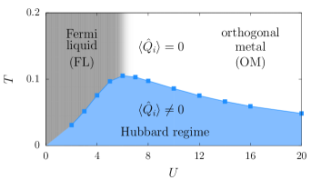
Figure 1: Phase diagram of the dual Hamiltonians (II.1), (6), and (9). A phase transition of the Ising variables $\hat{Q}_{i}$ at $T_{Q}$ separates the low-temperature Hubbard regime from the high-temperature phase. Here, $T_{Q}$ was determined from data for $L=8$, see Fig. 5. The two metallic regimes at $T>T_{Q}$ appear to be separated by a crossover, as indicated by the color gradient. Adapted from Ref. [34].

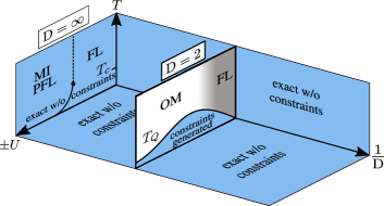
Figure 2: Schematic phase diagram of the Hubbard model in the unconstrained slave-spin representation defined by Hamiltonian (6) [equivalent to Hamiltonian (II.1)]. The axes correspond to the interaction $U$, the temperature $T$, and the inverse spatial dimension $1/\text{D}$. In the blue-shaded regions, the constraints $\hat{Q}_{i}$ from the slave-spin representation (identical to the local Ising variables in the FKM) are either irrelevant or dynamically generated so that the unconstrained models give the same results as the original Hubbard model. For $\text{D}=\infty$, paramagnetic DMFT yields a first-order phase transition from an FL to a Mott insulator (MI, repulsive case) or a paired Fermi liquid (PFL, attractive case) up to $T=T_{c}$, and a crossover (dashed line) for $T>T_{c}$ [35].

In Ref. [34], we introduced a Falicov-Kimball model (FKM) of spinful fermions with a three-body interaction. It reduces to the Hubbard model at low temperatures and in infinite dimensions. QMC simulations of this model revealed a rather interesting phase diagram, see Fig. 1. It features a line of thermal Ising phase transitions with critical temperature $T_{Q}(U)$, at which the localized degrees of freedom order ferromagnetically, and a crossover between two distinct metallic regimes at $T>T_{Q}$. The weak-coupling regime ($U\lesssim 6$) exhibits qualitatively FL-like properties, with thermodynamic and transport quantities determined by well-defined quasiparticles. This picture breaks down at stronger couplings where metallic behavior and gapless spin excitations coexist with a single-particle gap, highly reminiscent of OMs.

The connection to OMs and fractionalization can be made quite explicit via an exact duality between the FKM representation and a completely equivalent (i.e., dual) Z₂ slave-spin representation. In fact, our work began as an investigation of the Hubbard model in the slave-spin representation. QMC simulations reveal a clear correlation between the disappearance of quasiparticles and the disordering of the slave spins. As demonstrated below, in the low-temperature phase in Fig. 1, labeled Hubbard regime, the FKM has the same symmetry as the 2D Hubbard model and QMC results exhibit quantitative agreement. In fact, the duality reveals that the Ising variables of the FKM are exactly the constraints of the slave-spin representation. Considerations regarding the relevance of the latter lead to the generalized phase diagram of the unconstrained [36] slave-spin Hubbard model shown in Fig. 2 and discussed in Sec. II.

Here, we provide a significantly more detailed account of the different representations, the relevant symmetries, and the relation to the slave-spin theory of the Hubbard model. The distinct regimes of the phase diagram are characterized with a focus on $T>T_{Q}$. In particular, we study the temperature dependence of the compressibility, the conductivity, and the optical conductivity. The appearance of Hubbard physics at $T<T_{Q}$, but also the clearly non-Hubbard physics at $T>T_{Q}$, are illustrated. The results are followed by a discussion of the interpretation in terms of slave-spin theory and OMs, especially the differences between the present realization and mean-field theories or exactly solvable models.

The rest of this paper is organized as follows. In Sec. II we discuss the Hamiltonians. The QMC method is outlined in Sec. III. Numerical results are reported in Sec. IV, followed by a discussion in Sec. V. Finally, we conclude in Sec. VI.

II Model, dualities, symmetries

II.1 Hamiltonians

The square-lattice FKM introduced in Ref. [34] is defined by the Hamiltonian

$$\hat{H}^{cQ}= -t\sum_{\langle ij\rangle,\sigma}\left(\hat{c}^{\dagger}_{i\sigma}\hat{c}^{\phantom{{\dagger}}}_{j\sigma}+\text{H.c.}\right)$$

$$-U\sum_{i}\left(\hat{n}_{i\uparrow}-\mbox{$\frac{1}{2}$}\right)\left(\hat{n}_{i\downarrow}-\mbox{$\frac{1}{2}$}\right)\hat{Q}_{i}\,.$$ (1)

The first term describes the hopping of electrons with spin $\sigma$ between nearest-neighbor lattice sites $i$ and $j$ with amplitude $t$. The electrons couple to Ising degrees of freedom $\hat{Q}_{i}=\pm 1$ located at the sites with strength $U$. The density operator is defined as $\hat{n}_{i\sigma}=\hat{c}^{\dagger}_{i\sigma}\hat{c}_{i\sigma}$, the chemical potential $\mu=0$ for the case of half-filling ($\langle\hat{n}_{i}\rangle=\langle\hat{n}_{i\uparrow}+\hat{n}_{i\downarrow}\rangle=1$) considered here.

Writing the interaction as $U\sum_{i}\hat{Q}_{i}\prod_{\alpha}(\hat{n}_{i\alpha}-\mbox{$\frac{1}{2}$})$ with a flavor index $\alpha$, Eq. (II.1) may be regarded as a generalization of the spinless FKM with one flavor of itinerant fermions that can be solved exactly in infinite dimensions [37]. In fact, the original FKM of Ref. [38] was formulated with itinerant and localized SU(2) fermions, but does not contain a three-body interaction as in Eq. (II.1). The latter seems to preclude an exact solution but, as discussed in Sec. III, Hamiltonian (II.1) with $U>0$ is amenable to sign-free QMC simulations.

The connection to other FKMs becomes complete if the local Ising variables $\hat{Q}_{i}$ are expressed in terms of the occupation numbers of localized spinless fermions via

$$\hat{Q}_{i}=1-2\hat{n}^{l}_{i}=1-2\hat{l}^{\dagger}_{i}\hat{l}^{\phantom{{\dagger}}}_{i}\,.$$ (2)

This yields an onsite interaction $\sim U\hat{n}_{i\uparrow}\hat{n}_{i\downarrow}\hat{n}^{l}_{i}$.

Whereas we consider a half-filled band for the $c$ fermions, the number of $l$ fermions is determined by their interaction with the $c$ fermions and depends on $U$ and temperature. It is directly related to the magnetization of the $\hat{Q}_{i}$ variables. A ferromagnetic state with $\langle\hat{Q}_{i}\rangle=1$ ($\langle\hat{Q}_{i}\rangle=-1$) corresponds to $\langle\hat{n}^{l}_{i}\rangle=0$ ($\langle\hat{n}^{l}_{i}\rangle=1$), whereas a paramagnetic state with $\langle\hat{Q}_{i}\rangle=0$ implies $\langle\hat{n}^{l}_{i}\rangle=0.5$.

The representations based on either the fermion occupation numbers $\hat{n}^{\text{l}}_{i}$ or the Ising variables $\hat{Q}_{i}$ (both of which are conserved by the respective Hamiltonian) should yield identical results for $c$-fermion properties. However, only the fermionic representation reveals the nontrivial spectral properties of the $l$ fermions in the spinless FKM [39; 40; 41] via $\langle\hat{l}^{\dagger}_{i}(\tau)\,\hat{l}_{i}\rangle$ .

Figure 3: The relations between the Hamiltonians of Sec. II. The 2D FKM (II.1) is dual to an unconstrained slave-spin or lattice gauge theory that can be written either in terms of site Ising spins [Eq. (6)] or bond Ising spins [Eq. (9)]. If Gauss's law, defined by the local constraints (15), holds, Eqs. (6) and (9) become constrained gauge theories or, equivalently, exact slave-spin representations of the Hubbard model (10).

As illustrated in Fig. 3, the FKM (II.1) is related by an exact duality to a model of fermions coupled to Ising spins in a transverse field, which itself has two equivalent or dual representations. The first of these dual Hamiltonians is obtained by making the operator replacements

$$\hat{c}^{\dagger}_{i\sigma}\mapsto\hat{f}^{\dagger}_{i\sigma}\hat{s}^{z}_{i}\,,\quad\hat{c}_{i\sigma}\mapsto\hat{f}_{i\sigma}\hat{s}^{z}_{i}\,,$$ (3)

and

$$\hat{Q}_{i}=\hat{s}^{x}_{i}(-1)^{\sum_{\sigma}\hat{f}^{\dagger}_{i\sigma}\hat{f}_{i\sigma}}=\hat{s}^{x}_{i}(-1)^{\sum_{\sigma}\hat{c}^{\dagger}_{i\sigma}\hat{c}_{i\sigma}}\,,$$ (4)

where $\hat{f}^{\dagger}_{i\sigma}\hat{f}_{i\sigma}=\hat{c}^{\dagger}_{i\sigma}\hat{c}_{i\sigma}$ follows from Eq. (3). Here, $\hat{f}^{\dagger}_{i\sigma}$ creates a fermion with spin $\sigma$ at site $i$, whereas $\hat{s}^{z}_{i}$ and $\hat{s}^{x}_{i}$ are represented by Pauli matrices acting on an Ising spin at site $i$. Using the identity

$$(-1)^{\sum_{\sigma}\hat{f}^{\dagger}_{i\sigma}\hat{f}_{i\sigma}}=\prod_{\sigma}(2\hat{n}_{i\sigma}-1)$$ (5)

we can rewrite Eq. (II.1) as

$$\hat{H}^{fs}=-t\sum_{\langle ij\rangle,\sigma}\left(\hat{f}^{\dagger}_{i\sigma}\hat{f}^{\phantom{{\dagger}}}_{j\sigma}\hat{s}^{z}_{i}\hat{s}^{z}_{j}+\text{H.c.}\right)-\frac{U}{4}\sum_{i}\hat{s}^{x}_{i}\,.$$ (6)

Equation (6) has a dual representation in terms of fermions and bond Ising variables. The mapping between site Ising variables $\hat{s}^{\alpha}_{i}$ and bond Ising variables $\hat{\xi}^{\alpha}_{ij}$ is illustrated in Fig. 4. For nearest-neighbor sites $i$ and $j$,

$$\hat{s}_{i}^{z}\hat{s}^{z}_{j}\mapsto\hat{\xi}^{z}_{ij}\,.$$ (7)

Because a spin flip on a single site $i$ under the action of $\hat{s}^{x}_{i}$ affects all four bond variables, the dual representation involves a so-called star operator,

$$\hat{s}^{x}_{i}\mapsto\hat{\xi}^{x}_{i,i+x}\hat{\xi}^{x}_{i,i-x}\hat{\xi}^{x}_{i,i+y}\hat{\xi}^{x}_{i,i-y}\,,$$ (8)

where $i\pm\alpha$ is a compact notation for the site at $\bm{r}_{i}\pm\hat{e}_{\alpha}$. These steps lead to the Hamiltonian

$$\hat{H}^{f\xi}= -t\sum_{\langle ij\rangle,\sigma}\left(\hat{f}^{\dagger}_{i\sigma}\hat{f}^{\phantom{{\dagger}}}_{j\sigma}+\text{H.c.}\right)\,\hat{\xi}^{z}_{ij}$$ (9)

$$-\frac{U}{4}\sum_{i}\hat{\xi}^{x}_{i,i+x}\hat{\xi}^{x}_{i,i-x}\hat{\xi}^{x}_{i,i+y}\hat{\xi}^{x}_{i,i-y}\,.$$

Hamiltonian (9) with bond Ising variables $\hat{\xi}^{\alpha}_{ij}$ takes the form familiar from Ising lattice gauge theories coupled to matter. However, there are no additional constraints (also known as Gauss's law) in the context of the FKM. Such constraints arise in slave-spin representations (see Sec. II.2) and their role for the physics observed will be addressed in detail in Sec. V.

The origin of the lattice gauge theory (9) in a slave-spin representation implies the absence of $\pi$-flux configurations of the bond Ising variables. As illustrated in Fig. 4, on any closed loop, the sign of a site Ising variable $\hat{s}^{z}_{i}$ affects the sign of an even number of bond variables $\hat{\xi}^{z}_{ij}$ in the loop [cf. the star operator in Eq. (9)]. Therefore, the product of the $\hat{\xi}^{z}_{ij}$ over the loop will always equal $+1$, corresponding to the absence of a $\pi$ flux. Because of the link between site and bond variables, Eq. (7), the latter cannot be flipped individually. The absence of $\pi$ fluxes was accounted for in our simulations based on Eq. (9) by a proper choice of update rules, see Sec. III.

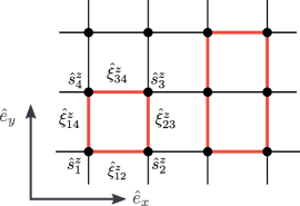
Figure 4: Relation between the bond Ising variables in Eq. (9) and the site Ising variables in Eq. (6). For any closed loop (indicated by thick red lines), $\prod_{\square}\hat{\xi}^{z}_{ij}=+1$ independent of the slave-spin configuration.

II.2 Relation to the slave-spin Hubbard model

The classification of the unusual metallic phase observed at $T>T_{Q}$ and $U\gtrsim 6$ (see Fig. 1) as a fractionalized metal is based on close conceptual relations with slave-spin theories and OMs. Most importantly, Eq. (9) is identical to the Ising (Z₂) slave-spin representation of the Hubbard Hamiltonian (we allow both interaction signs)

$$\hat{H}^{c}_{\pm}= -t\sum_{\langle ij\rangle,\sigma}(\hat{c}^{\dagger}_{i\sigma}\hat{c}^{\phantom{{\dagger}}}_{j\sigma}+\text{H.c.})\pm U\sum_{i}(\hat{n}_{i\uparrow}-\mbox{$\frac{1}{2}$})(\hat{n}_{i\downarrow}-\mbox{$\frac{1}{2}$})\,;$$ (10)

taking $U>0$, $\hat{H}^{c}_{+}$ ($\hat{H}^{c}_{-}$) corresponds to repulsive (attractive) interactions. This identification relies on the highly symmetric form of interactions in the FKM (II.1) with only a single interaction parameter $U$, in contrast to more general multi-component FKMs with independent interaction matrix elements and onsite energies [37; 36].

In complete analogy with Eq. (3), the idea of the slave-spin representation is to replace the original fermionic operators by auxiliary fermions $f$ and slave Ising spins $s$. The orientation of the slave spin at a given site is supposed to distinguish between doubly occupied and empty configurations on the one hand, and singly-occupied (local moment) configurations on the other hand. One of two possible choices is $\left|\uparrow\right\rangle^{s}_{i}\leftrightarrow n_{i}=0,2$ (even parity) and $\left|\downarrow\right\rangle^{s}_{i}\leftrightarrow n_{i}=1$ (odd parity), where $n_{i}$ is the eigenvalue of

$$\hat{n}_{i}=\sum_{\sigma}\hat{c}^{\dagger}_{i\sigma}\hat{c}^{\phantom{{\dagger}}}_{i\sigma}=\sum_{\sigma}\hat{f}^{{\dagger}}_{i\sigma}\hat{s}^{z}_{i}\hat{f}^{{\phantom{{\dagger}}}}_{i\sigma}\hat{s}^{z}_{i}=\sum_{\sigma}\hat{f}^{{\dagger}}_{i\sigma}\hat{f}^{{\phantom{{\dagger}}}}_{i\sigma}\,.$$ (11)

Because the hopping (interaction) term in Eq. (10) preserves (changes) the occupation number at the involved lattice sites, the slave-spin transformation is usually chosen as $\hat{c}^{({\dagger})}_{i\sigma}\mapsto\hat{f}^{({\dagger})}_{i\sigma}\hat{s}^{x}_{i}$. In the present work, we prefer to use the same form of the Hamiltonian throughout, and instead change the Ising quantization basis. Hence, we use the replacement

$$\hat{c}^{({\dagger})}_{i\sigma}\mapsto\hat{f}^{({\dagger})}_{i\sigma}\hat{s}^{z}_{i}\,,$$ (12)

which immediately yields the same hopping term as in Eq. (6). To make contact with the usual slave-spin picture, we can consider specifying the slave-spin orientation relative to the $x$ axis, thereby obtaining a diagonal Hubbard term. However, for the remainder of the paper, we exploit the freedom of switching back to the $z$ basis. This makes the hopping term diagonal in the slave spins and turns the Hubbard term into a transverse field, which facilitates our auxiliary-field QMC simulations. Moreover, the Hamiltonian (but not the physics) becomes identical to that considered in Refs. [43; 44].

In order to replace the Hubbard interaction by the simpler transverse-field term,

$$U\sum_{i}\left(\hat{n}_{i\uparrow}-\mbox{$\frac{1}{2}$}\right)\left(\hat{n}_{i\downarrow}-\mbox{$\frac{1}{2}$}\right)\mapsto\frac{U}{4}\sum_{i}\hat{s}^{x}_{i}\,,$$ (13)

we have to assume that the slave spin at a site $i$ faithfully describes the parity of $n_{i}$. Because auxiliary fermions and slave spins are formally independent, $[\hat{f}^{({\dagger})}_{i\sigma},\hat{s}^{\alpha}_{j}]=0$, the local Hilbert space in the slave-spin representation is

$$\mathcal{H}^{f}_{i}\otimes\mathcal{H}^{s}_{i}=\{\left|0\right\rangle_{i},\left|\uparrow\right\rangle_{i},\left|\downarrow\right\rangle_{i},\left|\uparrow\downarrow\right\rangle_{i}\}_{f}\otimes\{\left|\uparrow\right\rangle_{i},\left|\downarrow\right\rangle_{i}\}_{s}$$

and has a dimension twice as large as that of the original Hubbard model where $\mathcal{H}^{c}_{i}=\{\left|0\right\rangle_{i},\left|\uparrow\right\rangle_{i},\left|\downarrow\right\rangle_{i},\left|\uparrow\downarrow\right\rangle_{i}\}_{c}$. To select the four physical states and thereby achieve an exact representation of the Hubbard model, the slave-spin Hamiltonian (6) has to be supplemented with a local constraint on the corresponding eigenvalues. The latter can be formulated in several equivalent ways, including

$$\hat{s}^{x}_{i}-(-1)^{\hat{n}_{i}}\stackrel{{\scriptstyle!}}{{=}}0\,.$$ (14)

An alternative form, obtained by squaring Eq. (14), reveals a direct connection to the FKM:

$$\hat{Q}_{i}=\hat{s}^{x}_{i}(-1)^{\hat{n}_{i}}\stackrel{{\scriptstyle!}}{{=}}+1\,.$$ (15)

The choice $+1$ gives the above identification of $\left|\uparrow\right\rangle^{s}_{i}$ with $n_{i}=0,2$, whereas the physically equivalent choice $-1$ amounts to $\left|\downarrow\right\rangle^{s}_{i}$ representing $n_{i}=0,2$. In the FKM representation (II.1), the locally conserved $\hat{Q}_{i}$ may be replaced by classical variables $Q_{i}$. Their operator nature arises only after fractionalization of the $c$ fermions and is in particular reflected in the nontrivial commutation relations in Eq. (II.3) below.

The necessity of local constraints is a fundamental difference between the slave-spin representation of the Hubbard model and the corresponding transformation for the FKM that leads from Eq. (II.1) to Eq. (6). For the FKM, the local Hilbert space dimension remains unchanged, so that the transformation amounts to a mere relabeling of the states. Explicitly, for the FKM (II.1),

$$\mathcal{H}^{c}_{i}\otimes\mathcal{H}^{Q}_{i}=\{\left|0\right\rangle_{i},\left|\uparrow\right\rangle_{i},\left|\downarrow\right\rangle_{i},\left|\uparrow\downarrow\right\rangle_{i}\}_{c}\otimes\{\left|+1\right\rangle_{i},\left|-1\right\rangle_{i}\}_{Q}\,,$$

whereas for the fermion-spin model (6)

$$\mathcal{H}^{f}_{i}\otimes\mathcal{H}^{s}_{i}=\{\left|0\right\rangle_{i},\left|\uparrow\right\rangle_{i},\left|\downarrow\right\rangle_{i},\left|\uparrow\downarrow\right\rangle_{i}\}_{f}\otimes\{\left|\uparrow\right\rangle_{i},\left|\downarrow\right\rangle_{i}\}_{s}\,.$$

The unconstrained slave-spin representation of the Hubbard model is identical to the slave-spin representation (6) of the FKM (where no constraints arise). The addition of the constraints (15) promotes Hamiltonian (6) from an unconstrained gauge theory to a proper, constrained lattice gauge theory or, equivalently, an exact slave-spin representation of Eq. (10).

The fact that Eq. (15) resembles Eq. (4) for the FKM allows us to identify the Ising variables $\hat{Q}_{i}$ of the latter with the constraints of the slave-spin representation of the Hubbard model. Their role in ensuring a one-to-one mapping between Eqs. (10) and (6) becomes particularly clear from the observation that setting $\hat{Q}_{i}=1$ ($\hat{Q}_{i}=-1$) in Eq. (II.1) directly reduces the FKM to the attractive (repulsive) Hubbard model. In the context of the FKM, the constraints are spontaneously generated at the transition temperature $T_{Q}$, see Fig. 1. Therefore, at $T=0$, the FKM is equivalent to the Hubbard model or, alternatively, a constrained slave-spin gauge theory. In Sec. IV.2, we will demonstrate numerically that in the ferromagnetic phase at $T<T_{Q}$, the FKM does indeed yield results that are in quantitative agreement with those for the Hubbard model.

The fully polarized ferromagnetic state of the FKM is only one of several nontrivial limits in which an exact slave-spin or constrained lattice gauge representation emerges without explicitly imposing the constraints. In fact, in all the shaded regions in Fig. 2, the constraints are either irrelevant or dynamically generated and hence not necessary for a faithful representation of the Hubbard model. For example, for $U=0$, Eq. (II.1) immediately reveals that the $\hat{Q}_{i}$ play no role. As pointed out in Ref. [43], all $\hat{Q}_{i}$ sectors are degenerate in this limit. This is not only true for the ground state, as previously noted in Ref. [29], but at any temperature. Numerical evidence will be presented in Sec. IV.2.

Much more remarkably, the constraints are also irrelevant for any $U$ and $T$ in the limit of large spatial dimensions, $\text{D}=\infty$ [45]. Again, this becomes particularly transparent from the perspective of the FKM. A weak-coupling expansion of the partition function in powers of $\hat{H}_{1}=U\sum_{i}\left(\hat{n}_{i\uparrow}-\mbox{$\frac{1}{2}$}\right)\left(\hat{n}_{i\downarrow}-\mbox{$\frac{1}{2}$}\right)\hat{Q}_{i}$ takes the form

$$\frac{Z}{Z_{0}}=\sum_{n=0}^{\infty}\frac{(-1)^{n}}{n!}\left(\prod_{p=1}^{n}\int_{0}^{\beta}d\tau_{p}\right)\langle T\hat{H}_{1}(\tau_{1})\cdots\hat{H}_{1}(\tau_{n})\rangle\,.$$ (16)

The expectation value can be Wick-decomposed into all possible products of real-space single-particle propagators. However, for $\text{D}=\infty$, only the Hartree contributions are nonzero because nonlocal propagators vanish as $1/\sqrt{\text{D}}$ or faster [46; 47]. This leads to an effective Anderson impurity problem with a single interacting site $i_{0}$ to be solved self-consistently. At half-filling, only even powers $n=2m$ occur in the expansion (16) due to particle-hole symmetry. In combination with $i_{p}=i_{0}$ for all $p$, the constraints only enter in the form $(\hat{Q}_{i_{0}})^{2m}\equiv 1$ and the expansion reduces to that of the Hubbard model.

Because the constraints are irrelevant for $\text{D}=\infty$, the phase diagram of Fig. 2 for the unconstrained slave-spin theory of the Hubbard model [Eq. (6)] exhibits exactly the same Mott metal-insulator transition as found by dynamical mean-field theory (DMFT) for the repulsive Hubbard model (10) [48; 35; 30; 12]. In the slave-spin representation, the $T=0$ transition at $U_{c}>0$ is associated with a phase transition of the slave spins [30]. At $T>0$, a line of first-order transitions terminates at a critical endpoint at $T_{c}$, above which a metal-insulator (or FL to bad metal) crossover remains [48; 35; 30; 12].

II.3 Symmetries and their consequences

A look at the symmetries of the problem will prove useful for understanding the numerical results. First, the FKM (II.1) on the bipartite square lattice is invariant under the particle-hole transformation (acting on $\sigma=\uparrow,\downarrow$)

$$\hat{P}^{-1}\,\hat{c}^{\dagger}_{i\sigma}\,\hat{P}=\eta_{i}\hat{c}_{i\sigma}\,,\quad\hat{P}^{-1}\,\hat{c}_{i\sigma}\,\hat{P}=\eta_{i}\hat{c}^{{\dagger}}_{i\sigma}\,,$$ (17)

with the sublattice dependent phase factor

$$\eta_{i}=e^{\text{i}(\pi,\pi)\cdot\vec{r}_{i}}=\pm 1\,.$$ (18)

The SO(4)$=$SU(2)$\times$SU(2)/Z₂ symmetry of the Hubbard model, composed of SU(2) charge and spin symmetries [49], is present in the FKM as a subgroup of a larger O(4) symmetry. This follows from the fact that under the partial particle-hole or Shiba transformation [50], defined by

$$\hat{P}^{-1}_{{\sigma}}\,\hat{c}^{\dagger}_{i\sigma^{\prime}}\,\hat{P}_{{\sigma}}=\delta_{\sigma{\sigma}^{\prime}}\,e^{\text{i}(\pi,\pi)\cdot\vec{r}_{i}}\hat{c}_{i\sigma}+(1-\delta_{\sigma{\sigma}^{\prime}})\hat{c}^{\dagger}_{i\sigma}\,,$$ (19)

the hopping term remains unchanged but $U\to-U$ in the interaction term. The transformation hence connects repulsive and attractive Hubbard models, involving an interchange of charge and spin-$z$ operators [49]. In the FKM, we can compensate the sign change of $U$ by the global transformation $\hat{Q}_{i}\mapsto-\hat{Q}_{i}$. This constitutes an additional Z₂ symmetry (often referred to as parity or particle-hole symmetry) absent in the Hubbard model that restores the global $\text{SO}(4)\times\text{Z}_{2}=\text{O}(4)$ symmetry of free fermions. The latter implies, in particular, identical spin and charge correlation functions. Even though we explicitly choose an attractive interaction in Eq. (II.1) to avoid a QMC sign problem, the physics in the interesting O(4) symmetric regime at $T>T_{Q}$ is independent of the interaction sign.

The additional Z₂ symmetry is broken by the Hubbard term in Eq. (10). However, the Hubbard interaction in the slave-spin representation, $\hat{H}_{U}\sim\sum_{i}\hat{s}^{x}_{i}$, is invariant under an equivalent Shiba transformation for the $f$ fermions, leading to an O(4) symmetry at the level of Hamiltonian (6). For the Hubbard model, the constraints [Eq. (4) or Eq. (15)] change sign under $\hat{P}_{\sigma}$,

$$\hat{P}^{-1}_{{\sigma}}\,\hat{Q}_{i}\,\hat{P}_{{\sigma}}=-\hat{Q}_{i}\,,$$ (20)

since, for example, $\hat{P}^{-1}_{\uparrow}(-1)^{\sum_{\sigma}\hat{n}_{i\sigma}}\hat{P}_{\uparrow}=(-1)^{1-\hat{n}_{i\uparrow}+\hat{n}_{i\downarrow}}\,.$ Therefore, the constrained slave-spin representation has the same SO(4) symmetry as the original Hubbard Hamiltonian (10).

The additional Z₂ symmetry of the FKM is spontaneously broken at $T<T_{Q}$. In the Hubbard regime, we hence have the same SO(4) symmetry as for the Hubbard model. Similarly, the Z₂ symmetry can be broken by a magnetic field $-h_{Q}\sum_{i}\hat{Q}_{i}$ or, as in Sec. IV, by a Hubbard term. By the Mermin-Wagner theorem, spontaneous symmetry breaking in the fermionic sector only takes place at $T=0$, where the FKM has the same ground state as the Hubbard model: long-range AFM order for repulsive interactions ($\langle\hat{Q}_{i}\rangle=-1$) and combined CDW/SC order with an SO(3) order parameter for attractive interactions ($\langle\hat{Q}_{i}\rangle=+1$). In contrast, long-range order occurs also at $T>0$ in a recent DMFT study of Eq. (II.1) [51].

As suggested by the connection to lattice gauge theories, the slave-spin representation introduces a local Z₂ symmetry. We can change the sign of both $\hat{f}^{({\dagger})}_{i\sigma}$ and $\hat{s}^{z}_{i}$ while leaving $\hat{c}^{({\dagger})}_{i\sigma}=\hat{f}^{({\dagger})}_{i\sigma}\hat{s}^{z}_{i}$ unchanged. The generators of this transformation are the constraints $\hat{Q}_{i}$ with the property $\hat{Q}_{i}=\hat{Q}^{-1}_{i}$ since $\hat{Q}_{i}^{2}=1$. The local symmetry is reflected in

$$[\hat{H}^{fs},\hat{Q}_{i}]=[\hat{H}^{cQ},\hat{Q}_{i}]=0\,.$$ (21)

The operators in Eq. (6) transform as

$$\hat{f}^{({\dagger})}_{i\sigma} \mapsto\hat{Q}_{i}\hat{f}^{({\dagger})}_{i\sigma}\hat{Q}_{i}=-\hat{f}^{({\dagger})}_{i\sigma}\,,\quad$$

$$\hat{s}^{z}_{i} \mapsto\hat{Q}_{i}\,\,\hat{s}^{z}_{i}\,\,\hat{Q}_{i}=-\hat{s}^{z}_{i}\,.$$

$$\hat{s}^{x}_{i} \mapsto\hat{Q}_{i}\,\,\hat{s}^{x}_{i}\,\,\hat{Q}_{i}=+\hat{s}^{z}_{i}\,.$$ (22)

The $f$ fermions and the slave spins $\hat{s}^{z}_{i}$ carry a Z₂ charge, whereas $\hat{f}^{({\dagger})}_{i\sigma}\hat{s}^{z}_{i}\equiv\hat{c}^{({\dagger})}_{i\sigma}$ and $\hat{s}^{x}_{i}$ are neutral. Although invariance under local transformations is in the present setting related to an actual symmetry, the same operators appear in slave-spin theories and true gauge theories where the local transformations are associated with gauge invariance (choice of representation). Therefore, we will not strictly distinguish between Z₂ and gauge charges or Z₂ and gauge transformations.

According to Elitzur's theorem [52; 53], local symmetries cannot be spontaneously broken in finite dimensions at $T>0$. At $T=0$, symmetry breaking requires a macroscopic degeneracy of the ground state. This is realized at the critical point for the 1D Ising model [54]. However, in finite dimensions, we generally expect the third law of thermodynamics to hold and hence Elitzur's theorem to apply at any temperature.

The local symmetry imposes significant restrictions on correlation functions. Equation (21) yields

$$\hat{Q}_{i}\hat{f}^{({\dagger})}_{j}\hat{Q}_{i} =(1-\delta_{ij})\hat{f}^{({\dagger})}_{j}\,,$$

$$\hat{Q}_{i}\hat{s}^{z}_{j}\hat{Q}_{i} =(1-\delta_{ij})\hat{s}^{z}_{j}\,,$$ (23)

as well as $\hat{Q}_{i}\hat{s}^{x}_{j}\hat{Q}_{i}=\hat{s}^{x}_{j}$. Using Eqs. (15) and (II.3), $\hat{Q}_{i}^{2}=1$, as well as the cyclic invariance of the trace, leads to

$$\langle\hat{f}^{\dagger}_{i\sigma}(\tau)\hat{f}^{\phantom{{\dagger}}}_{j\sigma}(0)\rangle =\delta_{ij}\langle\hat{f}^{\dagger}_{i\sigma}(\tau)\hat{f}^{\phantom{{\dagger}}}_{i\sigma}(0)\rangle\,,$$

$$\langle\hat{s}^{z}_{i\sigma}(\tau)\hat{s}^{z}_{j\sigma}(0)\rangle =\delta_{ij}\langle\hat{s}^{z}_{i}(\tau)\hat{s}^{z}_{i}(0)\rangle\,.$$ (24)

Hence, correlation functions of gauge-dependent (charged) operators are entirely local in space. The key role of the local Z₂ symmetry in our model and in slave-spin theories will be discussed in Sec. V.3.

Finally, in contrast to Eq. (6), the FKM (II.1) contains only neutral operators and has a global Ising symmetry. A local U(1) symmetry (containing the Z₂ subgroup) emerges if the Ising variables are replaced by local fermions according to Eq. (2), reflecting invariance under the transformation $\hat{l}^{\dagger}_{i}\mapsto e^{\text{i}\varphi}\hat{l}^{\dagger}_{i}$, $\hat{l}^{\phantom{{\dagger}}}_{i}\mapsto e^{-\text{i}\varphi}\hat{l}^{\phantom{{\dagger}}}_{i}$ [37].

III Method

QMC simulations were carried out using the implementation of the auxiliary-field method from the Algorithms for Lattice Fermions (ALF) library [55]. This algorithm for correlated fermions goes back to the work of Blankenbecler et al. [56] and is based on a stochastic evaluation of the fermionic path integral with the help of discrete auxiliary fields. For a review see Ref. [57].

The simulations were done in the lattice-gauge representation (9). The partition function can be written as a Euclidean path integral over configurations $\bm{\xi}=\{{\xi}^{z}_{ij,\tau}\}$,

$$Z=\text{tr}\,e^{-\beta(\hat{H}-\mu\hat{N})}=\int\mathcal{D}[\bm{\xi}]\,e^{-S[\bm{\xi}]}\,.$$ (25)

As usual, imaginary time was discretized with a Trotter timestep $\Delta\tau=\beta/L$. The latter was typically fixed to $U\Delta\tau=0.1$, but much smaller values were used for simulations at high temperatures in order to have a sufficient resolution in imaginary time.

The configuration weight can be written as $e^{-S}=e^{-S_{0}}\det[1+B(\bm{\xi})]$. Here, the action $S_{0}$ describes the spin dynamics due to the transverse field, whereas $B$ is a product over time slices of exponentials of the hopping part that contains the fermion-spin coupling. Because $S$ is real, there is no sign problem for $U>0$.

An important distinction between the present problem and QMC simulations of Hubbard-Stratonovitch fields or fermions coupled to bond Ising spins is the fact that the bond spins $\hat{\xi}^{z}_{ij}$ are composed of two slave spins $\hat{s}^{z}_{i}$ and $\hat{s}^{z}_{j}$ at sites $i$ and $j$. Therefore, the minimal update consistent with the physics of the problem corresponds to flipping not one but all four bond spins connected to a given site. In particular, this ensures the absence of $\pi$-flux configurations. Since the bond spins determine the site spins only up to an overall sign, we stored a reference value $s^{z}_{1}$ for each configuration.

For the FKM (II.1), simulations in the bond-spin basis lead to a perfect sampling of the Ising variables $\hat{Q}_{i}$ and hence a symmetric distribution with $\langle\hat{Q}_{i}\rangle=0$. Because symmetry breaking only occurs for $L\to\infty$, our data therefore generally exhibit an O(4) symmetry unless the latter is broken explicitly. The results for the original Hubbard model in the standard fermionic representation were obtained using an SU(2) symmetric decomposition of the interaction [55].

Observables were measured using the single-particle Green function and Wick's theorem [57]. In addition to the gauge-invariant observables defined in terms of the original fermions, we also measured correlation functions of the slave spins $\hat{s}^{z}_{i}$. Dynamic correlation functions were accessible in imaginary time and analytically continued to real frequencies for selected parameters using the stochastic maximum entropy method of Ref. [58].

We work in units where $\hbar$, $k_{\text{B}}$, and $t$ are equal to one. All results are for square lattices with $L\times L$ sites and periodic boundary conditions.

IV Results

The presentation of our data is organized as follows. First, we recapitulate selected results of Ref. [34] to establish the key features of the phase diagram. Then, we demonstrate the emergence of Hubbard physics at $T<T_{Q}$, before turning to the two different metallic regimes at $T>T_{Q}$. Finally, we discuss similarities and differences with respect to the Hubbard model.

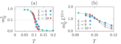
Figure 5: Ferromagnetic phase transition in the FKM with $U=6$ from the squared magnetization $m^{2}_{Q}$ [Eq. (26)]; $T_{Q}$ in Fig. 1 was obtained from the condition $m^{2}_{Q}(T_{Q}){=}0.5$, as illustrated in (a). (b) 2D Ising critical behavior with exponents $\beta=1/8$ and $\nu=1$. Figure adapted from Ref. [34].

IV.1 Structure of the phase diagram

As illustrated in Fig. 1, the numerical results support the existence of three distinct regimes in the $T$-$U$ phase diagram of the FKM (II.1). This structure reflects the central role of two different sets of Ising degrees of freedom in the problem—the constraints $\hat{Q}_{i}$ and the slave spins $\hat{s}^{\alpha}_{i}$—and their evolution with temperature and the transverse field $h\sim U$.

The critical temperature $T_{Q}(U)$ separates a high-temperature phase with O(4) symmetry and disordered Ising variables ($\langle\hat{Q}_{i}\rangle=0$) from a low-temperature phase with SO(4) symmetry and ferromagnetically ordered Ising variables ($\langle\hat{Q}_{i}\rangle\neq 0$). The phase transition originates from a fermion-mediated exchange interaction $J\sum_{ij}\hat{Q}_{i}\hat{Q}_{j}$ that is not forbidden by symmetry in Eq. (II.1) and will therefore be generated. The ferromagnetic order of the $\hat{Q}_{i}$ also lifts the macroscopic classical degeneracy at $T=0$ and thereby avoids a violation of the third law of thermodynamics [43].

In our finite-size simulations, the transition can be tracked by the square of the magnetization per site,

$$m_{Q}^{2}=\frac{1}{L^{2}}M^{2}_{Q}\,,\quad M^{2}_{Q}=\frac{1}{L^{2}}\sum_{ij}\langle\hat{Q}_{i}\hat{Q}_{j}\rangle\,.$$ (26)

Figure 5(a) reveals that $m^{2}_{Q}\to 1$ ($m^{2}_{Q}\to 0$) at low (high) temperatures. For simplicity, the critical temperatures in Fig. 1 were determined as those where $m^{2}_{Q}$ equals $0.5$. The comparison of $T_{Q}$ for different $L$ in Fig. 5(a) shows that finite-size effects are irrelevant for our purposes. Nevertheless, we demonstrate in Fig. 5(b) that a similar $T_{Q}$ is obtained from the crossing point in a proper finite-size scaling based on 2D Ising critical exponents $\beta=1/8$ and $\nu=1$.

The shape of the phase boundary in Fig. 5 is similar to that for the charge-density-wave (CDW) transition of the spinless FKM at half-filling observed both for $\text{D}=2$ and $\text{D}=\infty$ [37]. Exactly at $U=0$, the $\hat{Q}_{i}$ are decoupled and do not order, so $T_{Q}=0$. A nonzero coupling generates an exchange interaction $J$ between the $\hat{Q}_{i}$ and $T_{Q}\sim J$. For the spinless FKM, the exact solution in infinite dimensions gives $J=U^{2}|\ln U|$ at weak coupling and $J\sim t^{2}/U$ at strong coupling [59], suggesting $T_{Q}\to 0$ for $U\to\infty$ as in Fig. 1.

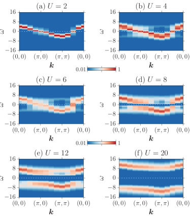
Figure 6: Single-particle spectral function $A(\bm{k},\omega)$ [Eq. (27)] of the FKM as a function of $U$. Here, $L=8$, $T=1/6$.

The existence of a crossover between two distinct metallic regimes with O(4) symmetry at $T>T_{Q}$ was established in Ref. [34] in terms of the results in Figs. 6 and 7. The single-particle spectral function

$$A(\bm{k},\omega) =-\frac{1}{\pi}\mathrm{Im}\,G(\bm{k},\omega)$$ (27)

was extracted from the spin-averaged Green function

$$G(\bm{k},\tau)=\mbox{$\frac{1}{2}$}\sum_{\sigma}\left\langle\hat{c}^{\dagger}_{\bm{k}\sigma}(\tau)\hat{c}^{\phantom{{\dagger}}}_{\bm{k}\sigma}(0)\right\rangle$$ (28)

using a maximum entropy method [58] to invert

$$G(\bm{k},\tau)=\int_{-\infty}^{\infty}\text{d}\omega\frac{e^{-\omega\tau}}{1+e^{-\beta\omega}}A(\bm{k},\omega)\,.$$ (29)

Figure 6 reveals gapless excitations for $U\lesssim 6$ (FL) but a gap at the Fermi level for $U\gtrsim 6$ (OM). The absence (presence) of a single-particle gap at weak (strong) coupling can also be inferred directly from the local imaginary-time Green function

$$G_{\text{loc}}(\tau)=\frac{1}{L^{2}}\sum_{\bm{k}}G(\bm{k},\tau)\,,$$ (30)

which is related to the density of states $N(\omega)$ by an identity akin to Eq. (28). The Green function is clearly finite at long times $\tau$ for small $U$ but exhibits an exponential decay determined by the single-particle gap at larger $U$.

At the same time, the persistence of metallic behavior at large $U$ is apparent from the current correlator

$${\Gamma}_{xx}(\bm{q},\tau)=\frac{1}{L^{2}}\sum_{\bm{r}\bm{r}^{\prime}}e^{-\text{i}(\bm{r}-\bm{r}^{\prime})\cdot\bm{q}}\left\langle\hat{\jmath}_{x}(\bm{r},\tau)\hat{\jmath}_{x}(\bm{r}^{\prime},0)\right\rangle$$ (31)

defined in terms of the current operator

$$\hat{\jmath}_{x}(\bm{r})=\text{i}\sum_{\sigma}\left(\hat{c}^{\dagger}_{\bm{r}+\hat{e}_{x},\sigma}\hat{c}^{\phantom{{\dagger}}}_{\bm{r}\vphantom{\hat{e}_{x}},\sigma}-\hat{c}^{\dagger}_{\bm{r},\sigma\vphantom{\hat{e}_{x}}}\hat{c}^{\phantom{{\dagger}}}_{\bm{r}+\hat{e}_{x},\sigma}\right)\,.$$ (32)

Although $\Gamma_{xx}(\tau)={\Gamma}_{xx}(\bm{q}=0,\tau)$ in Fig. 7(b) also exhibits a significant suppression with increasing $U$, it saturates at large $\tau$. This implies a Drude response ($\delta$ function at $T=0$, peak of finite width at $T>0$) and hence a nonzero conductivity in the thermodynamic limit. A detailed analysis of the (optical) conductivity and the resistivity will be given below.

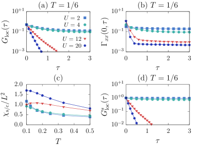
Figure 7: (a) Local single-particle Green function, (b) $\bm{q}=0$ current correlator, (c) identical charge and spin susceptibilities, and (d) slave-spin Green function of the FKM. Here, $L=8$. For clarity, (a),(b),(d) only show a subset of $\tau$ points.

A characteristic property of the OM regime is that despite the single-particle gap, long-wavelength spin fluctuations remain gapless (gapless charge fluctuations are naturally implied for a metallic phase). This is visible from the uniform susceptibilities

$$\chi_{\alpha}={\beta}\left(\langle\hat{O}_{\alpha}^{2}\rangle-\langle\hat{O}_{\alpha}\rangle^{2}\right)$$ (33)

for spin [$\hat{O}_{\text{s}}=\sum_{i}\hat{S}^{z}_{i}$, $\hat{S}^{z}_{i}=(\hat{n}_{i\uparrow}-\hat{n}_{i\downarrow})/2$] and charge ($\hat{O}_{\text{c}}=\sum_{i}\hat{n}_{i}$), which are identical for the FKM due to its O(4) symmetry. According to Fig. 7(c), $\chi_{\text{s}}$ and $\chi_{\text{c}}$ are slightly enhanced in the strong-coupling regime for $T>T_{Q}$, with a precursor effect of the Ising transition visible at the lowest temperatures for $U=12$. The curvature has a different sign in the FL and OM regime. Gapless spin and charge excitations have also been demonstrated in terms of the dynamic structure factor [34].

The evolution of the slave-spin Green function

$$G^{s}_{\text{loc}}(\tau)=\langle\hat{s}^{z}_{i}(\tau)\hat{s}^{z}_{i}(0)\rangle$$ (34)

with $U$ shown in Fig. 7(d) is very similar to that of the electronic Green function (28) in Fig. 7(a). It reveals a crossover from frozen, quasi-long-range correlations in imaginary time at small $U$ to short-ranged correlations at large $U$. The latter can be qualitatively captured in terms of a temporal ferromagnetic coupling $K=J/T=\text{arctanh}(e^{-\Delta\tau U/4})$. The correlation length of the corresponding 1D ferromagnetic Ising model is given by $(\ln\coth K)^{-1}\sim 1/U$.

IV.2 Hubbard physics from the FKM

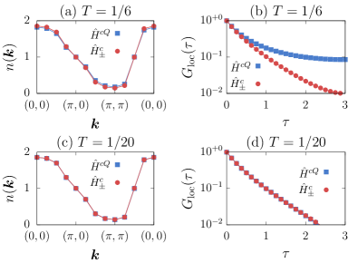
Figure 8: Comparison of (a), (c) the momentum distribution function and (b), (d) the local single-particle Green function for the FKM ($\hat{H}^{cQ}$) and the Hubbard model ($\hat{H}^{c}_{\pm}$) at (a), (b) high and (c), (d) low temperatures. Here, $U=6$, $L=8$.

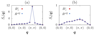
Figure 9: (a) Charge and (b) spin structure factor for the FKM ($\hat{H}^{cQ}$) with a magnetic field $h_{Q}=0.05$ and the attractive Hubbard model ($\hat{H}^{c}_{-}$). Here, $T=0.05$, $U=6$, and $L=8$.

According to Sec. II.2 and Fig. 2, the FKM (II.1) should exhibit quantitative agreement with the Hubbard model (10) in several parameter regions. To obtain explicit numerical evidence, we have to keep in mind that the spontaneous breaking of the relevant Z₂ symmetry only occurs in the thermodynamic limit. Our simulations in the representation (9) amount to a perfect sampling of the $\hat{Q}_{i}$, leading to an average over pairs of $\hat{Q}_{i}$ configurations related by a global spin flip $\hat{Q}_{i}\to-\hat{Q}_{i}$. Based on the discussion in Sec. II.2 and Eq. (II.1), this implies an average over the attractive and repulsive sectors of the Hubbard model that produces the O(4) symmetry. There are two routes to verify agreement with the Hubbard model in finite-size simulations: (i) considering observables that are invariant under the transformation (19) and hence identical for $U>0$ and $U<0$, (ii) breaking the O(4) symmetry explicitly.

Regarding the first possibility, we show in Fig. 8 the momentum distribution function

$$n(\bm{k})=\sum_{\sigma}\left\langle\hat{c}^{\dagger}_{\bm{k}\sigma}\hat{c}^{\phantom{{\dagger}}}_{\bm{k}\sigma}\right\rangle$$ (35)

and the local Green function defined in Eq. (30), which depend only on $|U|$. We take $U=6$, close to the maximum of $T_{Q}\approx 0.1$ in Fig. 1. While quantitative differences between the FKM and the Hubbard model are visible in both $n(\bm{k})$ and $G_{\text{loc}}(\tau)$ at $T=1/6>T_{Q}$ [Figs. 8(a) and (b)], results are essentially identical at $T=0.05<T_{Q}$ [Figs. 8(c) and (d)].

By adding a small magnetic field $h_{Q}$ for the $\hat{Q}_{i}$ or, equivalently, a small Hubbard interaction of strength $U^{\prime}=h_{Q}$ [cf. Eq. (10)], we can explicitly break the O(4) symmetry. This leads to quantitative agreement on finite systems, as illustrated in Fig. 9 for the charge and spin structure factors

$$S_{\text{c}}(\bm{q}) =\frac{1}{L^{2}}\sum_{ij}e^{-\text{i}(\bm{r}_{i}-\bm{r}_{j})\cdot\bm{q}}\left\langle(\hat{n}_{i}-1)(\hat{n}_{j}-1)\right\rangle\,,$$

$$S_{\text{s}}(\bm{q}) =\frac{1}{L^{2}}\sum_{ij}e^{-\text{i}(\bm{r}_{i}-\bm{r}_{j})\cdot\bm{q}}\left\langle\hat{S}^{z}_{i}\hat{S}^{z}_{j}\right\rangle\,,$$ (36)

A field $h_{Q}=0.05$ is sufficient to select the ferromagnetic phase with $\hat{Q}_{i}=1$ and thereby generate results that are identical to those for the attractive Hubbard model.

Finally, Fig. 10 demonstrates the asymptotic irrelevance of the constraints near $U=0$ at any temperature in terms of excellent agreement for the same observables as in Fig. 8 at a temperature $T=0.5\gg T_{Q}$.

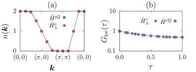
Figure 10: Comparison of (a) the momentum distribution function and (b) the local Green function for the FKM ($\hat{H}^{cQ}$) and the Hubbard model ($\hat{H}^{c}_{\pm}$). Here, $U=0.1$, $T=0.5$, and $L=8$.

IV.3 Metallic regimes at $T>T_{Q}$

At $T>T_{Q}$, the constraints $\hat{Q}_{i}$ are disordered, so that the FKM yields physics beyond the Hubbard model. Here, we first consider the crossover from the gapless FL to the gapped OM with increasing $U$, before turning to the temperature dependence.

IV.3.1 Crossover from weak to strong coupling

A crossover from the FL regime with well-defined quasiparticles to the OM regime without quasiparticles is suggested by Fig. 6. To substantiate this observation, we show in Fig. 11 the momentum distribution function [Eq. (35)] for different system sizes. While a true jump can only exist at $T=0$, the results for the FL regime at $U=4$ in Fig. 11(a) are consistent with the existence of quasiparticles. In contrast, in the OM regime at $U=12$ [Fig. 11(b)], the continuous dependence of $n(\bm{k})$ on $\bm{k}$ across the Fermi surface with essentially no finite-size effects supports the absence of quasiparticles.

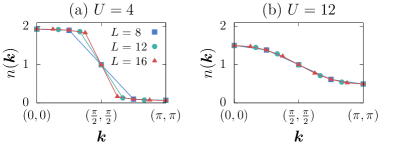
Figure 11: Momentum distribution function of the FKM at $T=1/6$ in (a) the FL and (b) the OM regime.

Previously [34], we calculated the dc conductivity using the estimator [60]

$$\sigma_{\text{dc}}^{(1)}\approx\frac{\beta^{2}}{\pi}{\Gamma}_{xx}(\beta/2)$$ (37)

(results in Ref. [34] include an additional factor $2$ from the trace ${\Gamma}_{xx}+\Gamma_{yy}$). An improved estimator that takes into account the curvature of ${\Gamma}_{xx}$ at $\tau=\beta/2$ is [61]

$$\sigma_{\text{dc}}^{(2)}\approx\frac{2\pi[{\Gamma}_{xx}(\beta/2)]^{2}}{\partial^{2}_{\tau}{\Gamma}_{xx}(\beta/2)}$$ (38)

and involves a quadratic fit near $\tau=\beta/2$ [61] (here, statistical errors were propagated but we did not quantify the impact of the fit range).

We also extracted $\sigma_{\text{dc}}$ from the real part of the optical conductivity $\sigma^{\prime}(\omega)$ via

$$\sigma_{\text{dc}}^{(3)}=\lim_{\omega\to 0}\sigma^{\prime}(\omega)\,.$$ (39)

This required a maximum-entropy inversion [58] of the Laplace transform

$${\Gamma}_{xx}(\tau)=\int\frac{\text{d}\omega}{\pi}\frac{e^{-\tau\omega}}{1-e^{-\beta\omega}}\omega\,\sigma^{\prime}(\omega)\,.$$ (40)

The f-sum rule for the optical conductivity reads [62; 63]

$$2\int_{0^{+}}^{\infty}\text{d}\omega\,\sigma^{\prime}(\omega)=-\pi e^{x}_{\text{kin}}-\rho_{\text{s}}$$ (41)

with the kinetic energy per bond ($t=1$)

$$e^{x}_{\text{kin}}=\frac{1}{2L^{2}}\sum_{\bm{r}\sigma}\langle\hat{c}^{\dagger}_{\bm{r}\vphantom{e_{x}}\sigma}\hat{c}^{\phantom{{\dagger}}}_{\bm{r}+\hat{e}_{x},\sigma}+\text{H.c.}\rangle$$ (42)

and the superfluid density $\rho_{\text{s}}$ defined in Eq. (43). We find that Eq. (41) holds numerically as long as $\sigma^{\prime}(\omega)$ does not have a very sharp low-energy feature that is nontrivial to reliably extract with the maximum-entropy method. Results for $\sigma^{\prime}(\omega)$ are shown despite non-negligible deviations (more than five percent) if only the qualitative structure is of interest. This applies to $U=2,4$ in Fig. 13(a) and to $T=1/6$ in Fig. 20(a). On the other hand, such data are excluded from the quantitative analysis of the dc conductivity in Figs. 12(b) and 19.

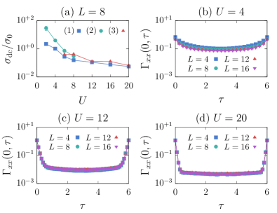
Figure 12: (a) Conductivity of the FKM from Eqs. (37) – (39). (b) – (d) Current correlator for different $L$. Here, $T=1/6$.

The accuracy of the estimators (37) and (38) depends on the spectral shape of $\sigma^{\prime}(\omega)$ and the temperature, see Refs. [60; 61; 14]. For example, $\sigma^{(1)}_{\text{dc}}$ gives reliable results if $\sigma^{\prime}(\omega)$ has no low-energy contribution sharper than $\Delta\omega\approx 8T$ [14]. The estimator (38) varies between $\sigma_{\text{dc}}$ for a single low-energy peak of width $\Delta\omega\gg T$ and $\sigma_{\text{dc}}/2$ for $\Delta\omega\ll T$ [14], but larger deviations are possible if $\sigma^{\prime}(\omega)$ has a different form. Similarly, $\sigma_{\text{dc}}$ values extracted from the maximum-entropy results for $\sigma^{\prime}(\omega)$ are subject to uncertainties that are challenging to quantify. At the same time, for the doped Hubbard model at high temperatures, qualitative or even quantitative agreement of different estimators was observed [14].

Here, the simplest but least accurate estimator (37) can be calculated for almost arbitrary parameters. In contrast, the use of Eq. (38) becomes challenging if $\Gamma_{xx}$ is flat around $\beta/2$, as is the case for large $U$ [see Fig. 7(b)]. Overall, while we cannot expect quantitative or even qualitative agreement, a comparison of all three estimators should reveal systematic trends.

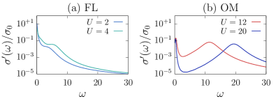
Figure 13: Optical conductivity of the FKM for $T=1/6$ and $L=8$. Here and in subsequent figures showing $\sigma^{\prime}(\omega)$, the energy resolution is $0.02$ and we applied a cubic Savitzky-Golay filter to obtain smooth(er) curves.

Figure 12(a) shows $\sigma_{\text{dc}}$ as a function of $U$ at $T=1/6$. The results reaffirm the findings of Ref. [34]: the conductivity drops sharply in the gapless weak-coupling regime, but much more slowly in the strong-coupling OM regime. At small $U$, the fact that $\sigma^{(1)}_{\text{dc}}$ underestimates the conductivity can be attributed to the significant variation of $\sigma^{\prime}(\omega)$ over $\omega\in[0,8T]$. In the OM regime, all three estimators yield quantitatively similar results. In total, we therefore see an even more pronounced difference between weak and strong coupling than in Ref. [34].

To rule out that the nonzero conductivity in the OM regime is merely a finite-size effect, Figs. 12(b) – (d) show the current correlation function for different system sizes $L$ in the FL and the OM regimes. Even in the FL regime [Fig. 12(b)], finite-size effects are minimal for the temperatures considered. In the OM regime, results for different $L$ are essentially identical and hence support a nonzero conductivity in the thermodynamic limit. This is of particular interest in connection with the 2D spinless FKM, for which metallic behavior has recently been argued to be absent at any $U>0$ for $L\to\infty$ [64], see Sec. V.

Figure 13 reveals the impact of the FL-OM crossover on the optical conductivity itself. At small $U$, where the single-particle spectrum is gapless [Figs. 6(a)–(b)], $\sigma^{\prime}(\omega)$ in Fig. 13(a) exhibits a dominant zero-frequency, Drude type contribution as well as a second peak centered at $\omega\approx U$. A reduced Drude response remains in the OM regime, Fig. 13(b), reflecting its metallic nature. Both the position ($\omega\sim U$) and height of the `Hubbard peak' remain largely unchanged. A significant shift of weight from zero to finite frequencies when comparing the weak and strong-coupling regimes is typical of strongly correlated systems [65]. The high-frequency peak is expected from the gap in the single-particle spectrum in Fig. 6. On the other hand, the low-frequency peak is entirely beyond a local theory without vertex corrections where a gap in $A(\bm{k},\omega)$ also implies a gap in $\sigma^{\prime}(\omega)$ [66].

An absence of critical behavior, in accordance with a crossover rather than a phase transition separating the FL and OM regimes, can be seen in Fig. 14. The inverse compressibility and the kinetic energy both vary smoothly with $U$ and exhibit only a very weak dependence on the system size $L$.

IV.3.2 Absence of superconductivity

While we interpret the gapped metallic regime at large $U$ in the framework of OMs, an apparent alternative explanation is superconductivity. The latter can be ruled out by calculating the superfluid density [67]

$${\rho_{\text{s}}}=\pi\left[-e^{x}_{\text{kin}}-\lim_{q_{y}\to 0}\Gamma_{xx}(q_{y})\right]\,.$$ (43)

Here, $\Gamma_{xx}(q_{y})\equiv\Gamma_{xx}(q_{x}=0,q_{y},\omega=0)$ corresponds to the integral of the current correlator defined in Eq. (31) over $\tau$. In a normal state, it is identical to the kinetic energy [Eq. (42)] so that $\rho_{\text{s}}=0$. Superconductivity implies a nonzero difference $\rho_{\text{s}}>0$ that has to be accounted for in the f-sum rule (41) [63].

Figure 15(a) shows that $\Gamma_{xx}(q_{y})$ approaches $-e^{x}_{\text{kin}}$ in the OM regime ($U=8$, $T=1/6$), indicating the absence of superconductivity. The same conclusion holds for larger values of $U$, as demonstrated in Fig. 15(b). Different behavior will be discussed below for the attractive Hubbard model.

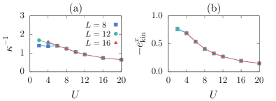
Figure 14: (a) Inverse compressibility and (b) resistivity from Eq. (37) of the FKM for different system sizes. Here, $T=1/6$.

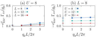
Figure 15: Transverse current response (filled symbols) and negative of the kinetic energy (open symbols) of the FKM in the OM regime at $T=1/6$.

IV.3.3 Temperature dependence

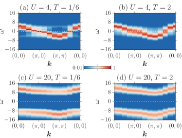
Figure 16: Single-particle spectral function of the FKM in (a),(b) the FL and (c),(d) the OM regime. Here, $L=8$.

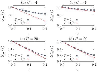
Figure 17: (a),(c) Local electron Green function and (b),(d) slave-spin Green function of the FKM for $L=8$.

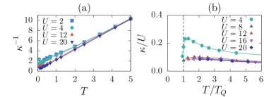
Figure 18: (a) Inverse compressibility of the FKM as a function of temperature. (b) Rescaled compressibility as a function of $T/T_{Q}$ with $T_{Q}$ from Fig. 1. Here, $L=8$.

The temperature dependence of quantities such as the resistivity and the optical conductivity is of particular interest in connection with experiments. For example, it distinguishes FLs from more exotic bad or strange metals [5]. For the FKM (II.1), Fig. 1 implies that regardless of methodological restrictions, the Ising transition at $T_{Q}$ does not permit us to track the temperature dependence of the OM all the way to $T=0$.

Figure 16 compares the spectral function $A(\bm{k},\omega)$ at low ($T=1/6$) and high temperatures ($T=2$) in the FL and OM regimes. Whereas for $U=4$ (FL) the gapless excitations become significantly broadened around the Fermi level, the spectrum remains virtually unchanged or becomes even slightly sharper at high temperatures for $U=20$ (OM).

The corresponding local Green functions of the $c$ fermions and the slave spins are shown in Fig. 17. In the FL regime, the impact of thermal fluctuations is significantly larger for the electrons [Fig. 17(a)] than for the slave spins [Fig. 17(b)] in terms of imaginary-time correlations at large $\tau$ that determine the gapless excitations in Fig. 16(a). This suggests that in the FL, the quasi-ordered slave spins do not fully determine the electronic excitations. In contrast, in the OM regime, both sectors exhibit very similar imaginary-time correlations and temperature effects. The robustness of the gapped, high-energy bands in $A(\bm{k},\omega)$ is reflected in an almost complete absence of thermal effects at small $\tau$ in Figs. 17(c) and (d). This can be attributed to the fact that the transverse field $h=U/4$ is much larger than the thermal energy $T$.

The charge susceptibility defined in Eq. (33) and shown in Fig. 7(c) is identical to the compressibility

$$\kappa=\frac{1}{\langle n\rangle^{2}}\frac{\partial\langle n\rangle}{\partial\mu}\,,$$ (44)

as can be readily established by differentiating the total particle number $N=L^{2}\langle n\rangle=\text{tr}(\hat{N}e^{-\beta(\hat{H}-\mu\hat{N})})/Z$ and setting $\langle n\rangle=1$. Independent of $U$, the inverse compressibility in Fig. 18(a) increases with temperature at high temperatures. However, as visible in Fig. 7(c), the FL and OM regimes are characterized by different signs of the curvature of $\kappa^{-1}$ at low temperatures. For $T>T_{Q}$, the compressibility is larger ($1/\kappa$ is smaller) in the OM than in the FL regime. The linear dependence at high temperatures can be understood in terms of the Curie behavior of quasi-free fermions.

Figure 18(a) shows $\kappa/U$ as a function of $T/T_{Q}$. As in a DMFT study of the same model [51], we find a significant dependence on $U$ in the FL regime but an approximate collapse of results for different $U$ in the OM regime. For $U=4$, where results are shown also for $T\lesssim T_{Q}$, Fig. 18(b) reveals a pronounced drop at the critical temperature (i.e., at $T/T_{Q}=1$). Hence, the Ising phase transition of the $\hat{Q}_{i}$, corresponding to a spontaneous symmetry reduction O(4)$\mapsto$SO(4), has a clear electronic signature, even though long-range order in the fermionic sector exists only at $T=0$. This is in strong contrast to the much smoother evolution of $\kappa^{-1}$ as a function of $U$ in Fig. 14(a), consistent with an FL-OM crossover rather than a phase transition.

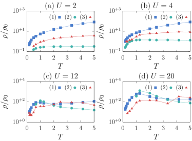
Figure 19: Resistivity of the FKM from the different estimators $\rho^{(i)}=1/\sigma_{\text{dc}}^{(i)}$ in (a), (b) the FL regime and (c), (d) the OM regime. Here, $L=8$.

Using the different conductivity estimators to calculate the resistivities $\rho^{(i)}=1/\sigma^{(i)}_{\text{dc}}$ reveals a larger variation among estimators than in Fig. 12(b). Nevertheless, the results in Fig. 19 exhibit interesting common trends. In the FL regime [Fig. 19(a)–(b)], $\rho$ increases strongly with temperature at low temperatures. For $T\gtrsim 1$, $\rho^{(1)}$ increases much more slowly whereas the other estimators suggest a saturating resistivity. Two distinct temperature regimes are also visible in the OM regime [Fig. 19(c)–(d)]. Here, $\rho$ is overall significantly larger than in the FL regime, in accordance with the conductivity in Fig. 12(b). The resistivity increases strongly with $T$ at low temperatures. The estimators $\rho^{(1)}$ and $\rho^{(2)}$ exhibit a maximum around $T=1$. Whereas $\rho^{(1)}$ remains essentially unchanged in the range $1\lesssim T\lesssim 5$, $\rho^{(2)}$ decreases with increasing temperature, suggesting a potential crossover from metallic to insulating behavior. The maximum at $T\approx 1$ is more pronounced for $U=20$ than for $U=12$. Finally, the maximum-entropy estimator $\rho^{(3)}$ is also consistent with a strong increase at low temperatures and saturation at high temperatures. The additional crossover from linear to quadratic behavior at low temperatures $T<0.5$ discussed in Ref. [34] cannot be addressed by estimators $(2)$ and $(3)$. Whereas the present results reveal saturation or even a decrease of the resistivity in the OM regime, a non-saturating resistivity and inverse compressibility were observed for the doped Hubbard model at comparable temperatures [13; 14].

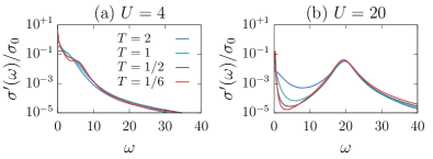
Figure 20: Optical conductivity of the FKM for (a) the FL regime and (b) the OM regime. Here, $L=8$.

The evolution of the optical conductivity with increasing $T$ can be seen in Fig. 20. In the FL regime at $U=4$ [Fig. 20(a)], the two separate peaks visible at low temperatures merge into a single peak at high temperatures, mainly due to the broadening of the Drude peak with increasing $T$. In contrast, in the OM regime at $U=20$ shown in Fig. 20(b), despite the filling-in of the spectral gap, two separate peaks remain clearly visible. The upper peak at $\omega\sim U$ shows only a minor shift to smaller frequencies with increasing $T$, in accordance with the slight reduction of the gap in Fig. 16. The ratio of spectral weights contained in the lower and upper peaks changes from about 1:4 at $T=1/6$ to 1:8 at $T=2$.

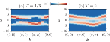
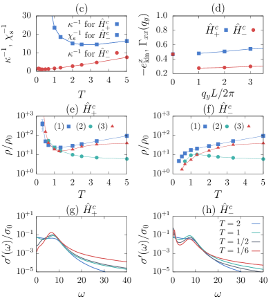
Figure 21: QMC results for attractive ($\hat{H}^{c}_{-}$) and repulsive ($\hat{H}^{c}_{+}$) Hubbard models. (a)–(b) Single-particle spectral function at (a) low and (b) high temperature, independent of the sign of $U$. (c) Inverse compressibility or (upon $\hat{H}^{c}_{-}\leftrightarrow\hat{H}^{c}_{+}$) inverse spin susceptibility, (d) transverse current response and kinetic energy, (e)–(f) resistivity from the three different estimators, and (g)–(h) optical conductivity for different temperatures. Here, $U=8$ and $L=8$.

IV.4 Differences to the half-filled Hubbard model

Given the relation of the FKM to the half-filled Hubbard model, we provide a brief comparison. To this end, we consider both attractive ($\hat{H}^{c}_{-}$) and repulsive ($\hat{H}^{c}_{+}$) interactions. The ground state changes qualitatively with the sign of the interaction but depends only quantitatively on the magnitude. Here, we focus on $U=8$, for which the relevant temperature and energy scales are readily accessible in QMC simulations.

At half-filling, the single-particle spectral function is independent of the sign of $U$. Its temperature dependence has been studied in detail before [68]. For $T$ above the magnetic scale $J=4t^{2}/U=0.5$ [Fig. 21(b)], the spectrum exhibits upper and lower Hubbard bands separated by a gap. In contrast, at $T<J$ [Fig. 21(a)], $A(k,\omega)$ has an intricate four-band structure not captured by the Hubbard I approximation. The additional features can be linked to the dressing of electron and hole excitations with coherent spin waves that emerge at low temperatures [68]. This can be contrasted with the FKM [Fig. 16(d)], where such physics is absent at $T>T_{Q}$.

The inverse compressibility in Fig. 21(c) reveals the suppression of charge fluctuations for repulsive interactions, as opposed to the attractive case. For the latter, the behavior of $\kappa^{-1}$ is qualitatively similar to the OM regime, cf. Fig. 18(b). By the transformation (19), $\kappa^{-1}$ for the repulsive (attractive) Hubbard model is also identical to the uniform spin susceptibility of the attractive (repulsive) Hubbard model. Hence, Fig. 21(c) reveals an exponential decrease of $\chi_{\text{s}}$ of the attractive model due to spin gap formation, whereas spin excitations remain gapless for repulsive interactions. The spin gap is perhaps the most pronounced difference between the attractive Hubbard model at $T>0$ and the FKM in the OM regime [Fig. 7(c)].

In contrast to the FKM (Fig. 15), the attractive Hubbard model exhibits signatures of superconductivity (note that $T_{c}=0$ at half-filling [69]). Whereas the kinetic energy is independent of the sign of $U$, the transverse current response in Fig. 21(d) reveals a nonzero superfluid density for $\hat{H}^{c}_{-}$ that contributes to the sum rule (41). Because this component is not captured by $\sigma^{\prime}(\omega)$, the corresponding results for $\rho$ based on estimator (3) are excluded from Fig. 21(f).

The resistivity, shown in Figs. 21(e) and (f), is thermally activated for attractive and repulsive interactions at $T\gtrsim 1$. At lower temperatures, the attractive (repulsive) model shows metallic (insulating) behavior. Comparison of Fig. 21(f) with Fig. 19(c) reveals that $\rho(T)$ of the attractive Hubbard is qualitatively similar to the FKM results. Finally, the optical conductivity in Figs. 21(g) and (h) has a Hubbard peak for both signs of the interaction. Whereas the optical conductivity looks markedly different for $U>0$ and $U<0$ at low temperatures, the filling-in (suppression) at low frequencies in the repulsive (attractive) case lead to almost identical results at high temperatures.

V Discussion

In this section, we first summarize the mean-field theory that underlies the identification of the strong-coupling metallic regime as an OM, before discussing the similarities and differences in the present case. We then address the role of the gauge symmetry and quantum fluctuations, and connections to other problems.

V.1 Mean-field theory and orthogonal metals

Our discussion follows Ref. [31] but we use the notation of Sec. II.2. More details and applications can be found in Refs. [29; 31; 70; 71]. A product ansatz for the ground state of Hamiltonian (6) of the form

$$\left|\Phi\right\rangle_{\text{MF}}=\left|\phi\right\rangle_{f}\otimes\left|\phi\right\rangle_{s},\$$ (45)

decouples the problem into a free-fermion part

$$\hat{H}_{\text{MF}}^{f}=-{t}\sum_{\langle ij\rangle,\sigma}g_{ij}(\hat{f}^{\dagger}_{i\sigma}\hat{f}^{\phantom{{\dagger}}}_{j\sigma}+\mathrm{H.c.})$$ (46)

and a transverse-field Ising model

$$\hat{H}_{\text{MF}}^{s}=-t\sum_{\langle ij\rangle}J_{ij}\hat{s}^{z}_{i}\hat{s}^{z}_{j}-\frac{U}{4}\sum_{i}\hat{s}^{x}_{i}\,$$ (47)

with the self-consistency conditions

$$g_{ij}=\langle\hat{s}^{z}_{i}\hat{s}^{z}_{j}\rangle_{s}\,,\quad J_{ij}=\sum_{\sigma}\langle(\hat{f}^{\dagger}_{i\sigma}\hat{f}^{\phantom{{\dagger}}}_{j\sigma}+\mathrm{H.c.})\rangle_{f}\,.$$ (48)

In the simplest case, these expectation values are the same for all nearest-neighbor bonds $\langle ij\rangle$. A more elaborate mean-field approach with a larger unit cell can be found, e.g., in Ref. [70]. Because the notation for the expectation values in Eq. (48) is specific to an ansatz such as Eq. (45), we drop the indices $s$ and $f$ from here on.

In the context of slave-spin theories, Eqs. (46)–(47) have to be supplemented with local constraints [29; 31; 31]. This is not the case if we consider Eq. (6) as the dual (unconstrained slave-spin) representation of the FKM (II.1).

The quadratic fermionic part can be solved exactly for given $g_{ij}$ and describes noninteracting fermions. The slave-spin part may be solved by single-site or cluster mean-field methods [29]. Alternatively, more advanced schemes based on saddle-point expansions or even numerical simulations are possible [72]. At any rate, the physics of the 2D quantum Ising model (47) is well understood. Hamiltonian (47) has a ferromagnetic (since $-tJ_{ij}>0$) ground state with $\langle\hat{s}^{z}_{i}\rangle\neq 0$ for $U<U_{c}$ and a paramagnetic ground state with $\langle\hat{s}^{z}_{i}\rangle=0$ for $U>U_{c}$, separated by a phase transition.

The effect of this phase transition on the original $c$ electrons becomes apparent from their spectral function. The latter is a convolution of the $f$-electron spectrum with that of the slave spins [31],

$$A(\bm{k},\omega)=\int\text{d}\bm{q}\int\text{d}\Omega\,A^{f}(\bm{q},\Omega)A^{s}(\bm{k}-\bm{q},\omega-\Omega)\,.$$ (49)

In the ordered phase, it takes the form [31]

$$A(\bm{k},\omega)=\langle\hat{s}^{z}_{i}\rangle^{2}\delta(\omega-E_{\bm{k}})\,.$$ (50)

Here, the $\delta$ peak signals the absence of interactions in the $f$-fermion sector and $\langle\hat{s}^{z}_{i}\rangle^{2}$ can be identified with the $c$-fermion quasiparticle residue. The latter vanishes on approaching the magnetic transition at $U_{c}$ and hence takes the role of a fermionic order parameter. In the paramagnetic phase of the slave spins, $A^{s}$ and therefore also $A$ have a gap [31].

As pointed out in Ref. [31], earlier interpretations of the slave-spin transition as a Mott transition of the $c$ fermions are in general not correct. Unless vertex corrections can be neglected (as is the case in infinite dimensions), a gap in $A(\bm{k},\omega)$ does not imply a vanishing conductivity. Within the above mean-field theory, transport is fully determined by the noninteracting Hamiltonian (46). The Drude weight ${D}\sim g_{ij}=\langle\hat{s}^{z}_{i}\hat{s}^{z}_{j}\rangle$ [31] is nonzero as long as the slave spins have nonlocal correlations. It is only within local mean-field theories, where $\langle\hat{s}^{z}_{i}\hat{s}^{z}_{j}\rangle=\langle\hat{s}^{z}_{i}\rangle^{2}$, that a vanishing quasiparticle weight coincides with $D=0$ and hence insulating behavior. Therefore, beyond local approximations, the gapped paramagnetic phase is not a Mott insulator but a metallic state with a single-particle gap, namely the OM [31]. Transport is fully carried by the gapless $f$ electrons that may be regarded as being orthogonal to the gapped $c$ fermions. This emerges naturally from the fact that the $f$ fermions inherit both the physical spin [SU(2) symmetry] and the physical charge [U(1) symmetry] of the original fermions [31].

V.2 Classification as an orthogonal metal

The classification of the gapped regime at $T>T_{Q}$ and $U\gtrsim 6$ as an OM can be motivated from the duality between the FKM (II.1) and the slave-spin representation (6) in conjunction with the evolution of the slave-spin Green function in Fig. 7(d). Whereas this connection requires some explanation with respect to the absence of symmetry breaking beyond mean-field theory (see below), we also observe the defining OM properties directly in the FKM representation: an absence of quasiparticles [Figs. 6(d)–(f) and 11(b)] together with a nonzero conductivity [Fig. 12(b)], spin and charge susceptibility [Fig. 7(d)]. They key role of the single-particle spectral function in distinguishing FL and OM regimes [31] is fully borne out by our numerical results.

For weak $U$, the existence of well-defined quasiparticles [Figs. 6(a)–(b) and 11(a)] is consistent with an FL, for which the density of states $N(E_{\text{F}})$ determines, e.g., the spin susceptibility [73]. In contrast, for large $U$, the Drude peak in Fig. 13(b) and the associated nonzero conductivity [Fig. 12(b)] cannot be reconciled with the absence of quasiparticles within FL theory. Whereas the $f$ fermions remain noninteracting in the models of Refs. [31; 33; 74], the existence of orthogonal phases with residual interactions can readily be conceived.

In Sec. IV.4, we showed that some properties of the OM (single-particle gap, nonzero conductivity) are also realized in the attractive Hubbard model at $T>T_{c}$ ($T_{c}=0$ for the case of half filling considered). The key distinction was the existence of a gap for spin excitations in the latter, corresponding to a paired FL or a pseudo-gapped metal. In contrast, the OM in the FKM has gapless spin excitations, demonstrated in terms of the spin susceptibility [Fig. 7(c)] and the dynamic spin structure factor [34]. A spin gap gives rise to an entirely non-FL spin susceptibility that decreases exponentially at low temperatures. Therefore, and given the absence of $f$-fermion interactions that could produce such a gap in their models, it is surprising that systems with uncondensed pairs of fermions are suggested as candidates for OMs in Ref. [31]. In contrast, our work appears to provide a faithful realization of the fermionic OM deduced from mean-field theory.

Despite the close similarities with OMs in terms of gauge-invariant properties, distinctions remain at the level of quantum numbers in the unconstrained slave-spin formulation (6) of the FKM (II.1). In the latter, the Z₂ charge is conserved in space but not in time. This should be compared with the exactly solvable fermion-spin models of Refs. [31; 33] that have no local symmetry and hence no associated Z₂ charge. It is also different from $T=0$ numerical realizations of orthogonal (semi-)metals with spontaneously generated constraints [43; 44; 75; 74].

To elucidate this point, we first note that according to Eq. (21), Hamiltonian (6) conserves the $\hat{Q}_{i}$ and can therefore be represented in terms of blocks (Z₂ charge or superselection sectors) corresponding to fixed configurations of the $\hat{Q}_{i}$ [36]. Whereas the physical sector (e.g., $\hat{Q}_{i}=1$ for all $i$) is selected in constrained theories, all possible sectors contribute to the physics observed at $T>T_{Q}$.

If we only consider hopping processes, the Z₂ charge remains conserved because the hopping term in Eq. (6) changes both the fermion parity and the slave-spin orientation at each of the sites involved. This is illustrated in terms of world lines of the $f$ fermions and the slave spins in Figs. 22(a)–(c). Even though $\hat{s}^{x}_{i}(-1)^{\hat{n}_{i}}$ and $\hat{Q}_{i}$ are not linked at $T>T_{Q}$, they both retain their value along the imaginary time axis. If constraints hold, all sites will have the same value of $\hat{Q}_{i}$ corresponding to the physical subspace chosen for the slave-spin representation. Hence, with respect to hopping, constrained and unconstrained theories are distinguished only by the values of the $\hat{Q}_{i}$. The latter have trivial flat world lines as a result of Eq. (21) and are therefore not shown in Fig. 22. In contrast, the Ising degrees of freedom in Eqs. (6) and (9) have a nontrivial dynamics determined by the transverse-field term $\sim U$.

Constrained and unconstrained theories clearly differ with respect to local fluctuations of the occupation of the Z₂ charged $f$ fermions, as illustrated in Figs. 22(d)–(f). In constrained theories, Gauss's law ensures that changes of the $f$-fermion number entail corresponding changes of the slave spins to preserve the eigenvalues of $\hat{Q}_{i}$ [Fig. 22(e)]. In contrast, without constraints, the slave-spin configuration remains unchanged in Fig. 22(f), mimicking a transition between different charge sectors as a function of imaginary time and corresponding to a violation of Z₂ charge conservation.

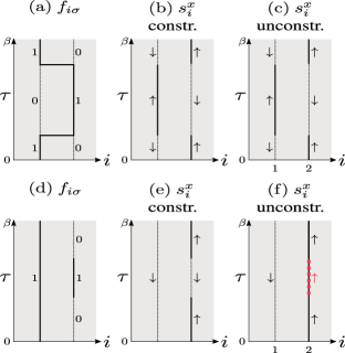
Figure 22: World-line configurations of $f$ fermions and slave spins that illustrate the conservation or non-conservation of the Z₂ charge under (a)–(c) hopping and (d)–(f) imaginary-time particle number fluctuations. (a) and (d) include occupation numbers without reference to the fermion spin $\sigma$.

V.3 Gauge-invariant picture

The above mean-field theory of the FL-OM transition provides a conceptual framework to understand our numerical findings. In particular, the significantly different behavior of the slave spins at weak and strong coupling justifies the fractionalization ansatz (12). At the same time, the mean-field results require some clarification in the context of gauge invariance and our numerical simulations. Although the connections between the FKM (II.1) and the Hubbard model are of significant interest, we point out that a constrained slave-spin representation of the former is not desirable because it would produce known Hubbard results at any temperature, which are more easily accessible in the representation (10).

To be concrete, we focus on the repulsive Hubbard model, even though our considerations apply more generally. The theory of Sec. V.1 suggests a $T=0$ FL-OM transition associated with a phase transition of the slave Ising spins driven by the transverse field $h=U/4$. The ferromagnetic phase corresponds to the FL, the paramagnetic phase to the OM. In contrast, the true ground state of the 2D Hubbard model and the FKM (II.1) (equivalent to the Hubbard model at $T=0$) is known to be an antiferromagnetic Mott insulator for any $U>0$. The paramagnetic phase of the mean-field description reduces to a Mott insulator in the local approximation, but the theory does not capture the magnetic order or the weak-coupling instability due to perfect nesting. Clearly, mean-field slave-spin approaches have rather limited predictive power for specific models.

As discussed in Sec. II.3, a gauge redundancy (constrained theories) or local symmetry (unconstrained theories), inherent to the slave-spin representation of Eq. (6), implies that expectation values of gauge-dependent operators vanish. Elitzur's theorem [52] generally rules out a spontaneous breaking of gauge invariance or local symmetries in finite dimensions.

The local Z₂ transformations are generated by the $\hat{Q}_{i}$. In an exact slave-spin treatment (constrained gauge theory, or unconstrained theory below $T_{Q}$), they can be applied at any point in spacetime [53]. This implies

• the absence of a phase transition of the slave spins characterized by a local order parameter,

• the absence of any nonlocal spatial or temporal correlations of $f$ fermions or slave spins.

For constrained and unconstrained theories, the fact that $\hat{s}^{z}_{i}$ and $\hat{f}^{({\dagger})}_{i\sigma}$ carry a gauge charge requires that the magnetization $m=\langle\hat{s}^{z}_{i}\rangle$, the mean-field Drude weight $D\sim\langle\hat{s}^{z}_{i}\hat{s}^{z}_{j}\rangle$, and $\langle\hat{f}^{\dagger}_{i\sigma}\hat{f}^{\phantom{{\dagger}}}_{j\sigma}\rangle$ vanish. For example, using Eq. (II.3) directly yields

$$m=\langle s^{z}_{i}\rangle=\langle\hat{Q}_{i}s^{z}_{i}\hat{Q}_{i}\rangle=-\langle s^{z}_{i}\rangle=0\,.$$ (51)

For the Hubbard model, imposing these restrictions on the slave-spin mean-field theory would yield a Mott insulator for any $U>0$.

A more appropriate interpretation of the mean-field results comes from lattice gauge theories, where predictions based on a forbidden local order parameter are often in good agreement with more advanced gauge-invariant approaches [76; 77]. For example, the ferromagnetic order of the slave spins in the FL regime may be regarded as obtained for a fixed gauge [the product ansatz (45) reduces the local gauge symmetry to a global Z₂ symmetry]. If the different saddle points related by gauge transformations make similar contributions to gauge-invariant quantities, averaging will yield nontrivial results while restoring gauge invariance. The symmetry-forbidden expectation values are hence merely the mean-field encoding of gauge-invariant physics. More generally, the physics extracted by gauge-fixing can also be observed in a gauge-invariant formulation [76; 77]. Here, the unconstrained and hence not fully gauge-invariant representation (6) has a dual, manifestly gauge-invariant representation in terms of the FKM (II.1). Similarly, OMs can be observed in exactly solvable models that do not have a local Z₂ symmetry [31; 33] as well as in numerical simulations of gauge theories coupled to matter with spontaneously generated constraints [75; 74].

For the FKM (II.1), as well as other unconstrained gauge theories, nontrivial imaginary-time correlations of gauge-dependent operators are explicitly allowed and observed because point (ii) above only applies to spatial correlations. For example, the temporal freezing of the slave spins at $U=0$ can mimic long-range order on the relevant time scales while preserving a vanishing (spatial) magnetization. An adiabatic connection between $h=0$ and $h>0$ has been established for the Higgs phase of Ising lattice gauge theories [78].

The crossover from frozen to disordered slave spins tracks the opening of the single-particle gap and the associated breakdown of a quasiparticle description. (This is opposite to non-FL physics arising from spin-freezing [79].) However, it does not account for the pronounced differences between paramagnetic Mott and OM phases. Whereas the former is a fully gauge-invariant state determined by local physics, the latter crucially relies on vertex corrections, encoded at the mean-field level in the nonvanishing spatial correlators $\langle\hat{s}^{z}_{i}\hat{s}^{z}_{j}\rangle$ and $\langle\hat{f}^{\dagger}_{i\sigma}\hat{f}^{\phantom{{\dagger}}}_{j\sigma}\rangle$. Such physics is fully captured by our numerical simulations, but absent in the DMFT limit $\text{D}=\infty$ where the OM is replaced by a Mott insulator. For $\text{D}=\infty$, both spatial and temporal correlations are allowed by Elitzur's theorem [80]. However, spatial correlations and vertex corrections are generically absent, resulting in a strong time-space asymmetry of gauge-dependent correlators similar to the 2D FKM (II.1). Although vertex corrections may be expected to be less important at high temperatures, DMFT does not become exact for $T\to\infty$ [13]. This is consistent with our observation of an OM at high temperatures but its absence in DMFT.

An interesting question is whether the FL and OM regimes are connected by a phase transition or a crossover. Whereas the mean-field scenario with the local order parameter $\langle\hat{s}^{z}_{i}\rangle$ violates gauge invariance, it is known that in $2+1$ dimensions the Ising lattice gauge theory is dual to the standard Ising model with a global Z₂ symmetry [81]. The phase transition of the latter is encoded in the former in terms of the different behavior (area vs. perimeter law) of the Wegner-Wilson loop correlator [81; 53; 8], a nonlocal gauge-invariant order parameter. Whether such a transition survives for nonzero matter coupling and at finite temperature cannot be answered in general. For example, a 3+1D Ising theory coupled to a Higgs field exhibits a first-order transition (crossover) below (above) a critical Higgs mass [82]. Our numerical data appear consistent with an FL-OM crossover driven by the disordering of the slave-spins and with a smooth evolution of gauge-invariant properties. A continuous FL-OM quantum phase transition, characterized by a nonlocal order parameter, was numerically realized for a Z₂ gauge theory in Ref. [74].

A phase transition of the slave spins with a local order parameter is observed at $T=0$ for $\text{D}=\infty$ [30], where it is not forbidden by Elitzur's theorem [80]. Because the constraints are irrelevant, the paramagnetic DMFT solution of the unconstrained slave-spin theory gives exact results and $\langle\hat{s}^{z}_{i}\rangle$ serves as an order parameter [30]. However, in the absence of vertex corrections, the OM is replaced by a Mott insulator, see Fig. 2. Even for $\text{D}=\infty$, the mean-field picture apparently breaks down at $T>0$, where DMFT suggests a vanishing slave-spin magnetization for all $U$. As pointed out in Ref. [30], this is consistent with an identification of the slave-spin magnetization with the quasiparticle weight, the latter being defined only at $T=0$. In DMFT, the first-order Mott transition in Fig. 2 is instead characterized by the opening of a gap in the slave-spin spectrum [30], quite similar to the disordering crossover observed here (frozen slave spins imply gapless excitations).

While the slave-spin magnetization is gauge-dependent and hence zero for $\text{D}<\infty$, mean-field theory establishes a link to the gauge-invariant quasiparticle residue. The latter is given by the jump of $n(\bm{k})$ at $T=0$ but vanishes for $T>0$. A more general gauge-invariant order parameter is $\langle\hat{s}^{x}_{i}\rangle$; $\hat{s}^{x}_{i}$ may be regarded as a disorder operator [83] whose condensation amounts to a proliferation of domain walls in imaginary time and hence a disordering of the slave spins. The data for the slave-spin Green function in Fig. 7(d) can qualitatively be understood as a crossover from $\langle\hat{s}^{x}_{i}\rangle=0$ at small $U$ to $\langle\hat{s}^{x}_{i}\rangle>0$ at large $U$.

For $\text{D}=\infty$, or in constrained slave-spin theories, $\langle\hat{s}^{x}_{i}\rangle$ is directly related to the fermion double occupancy $\langle\hat{n}_{i\uparrow}\hat{n}_{i\downarrow}\rangle$, see Eq. (13). The latter is manifestly gauge invariant and provides an experimentally accessible [84] Ising order parameter for the Mott transition also at $T>0$ [85; 86; 48; 87]. The O(4) symmetry of the FKM (II.1) implies that the double occupancy is independent of $U$, corresponding to an average over the values for the attractive and the repulsive Hubbard model. However, it is not clear if this should be interpreted as evidence for a crossover rather than a phase transition, as done in Ref. [51]. A crossover scenario is favored by the smooth evolution and absence of noticeable size effects in Fig. 14, as opposed to the clear signature of the magnetic phase transition (FL to Hubbard regime) in Fig. 18(b). Although the OM is distinguished from a Mott state by nonlocal effects, the generically weak finite-size effects in Figs. 11(b), 12(c), 12(d), and 14 suggest predominantly short-range correlations.

V.4 Z₂ fractionalization and topological order

Slave-spin mean-field theories have also been applied to models of interacting fermions with topologically nontrivial band structures. Such approaches yield Z₂-fractionalized quantum spin Hall (QSH) and Chern insulators [70; 71]. Here, we focus on the so-called QSH* phase reported for a Hubbard model with spin-orbit coupling [70]. It is separated from the regular QSH phase by an Ising transition of the slave spins. In the QSH* phase, where the slave spins are disordered, the characteristic helical edge states [88] are gapped in terms of the $c$ fermions but remain metallic with respect to the $f$ fermions. The prospect of such a phase—absent in unbiased simulations of the Kane-Mele-Hubbard model [89]—partially motivated our work.

The classification of the QSH* phase as topologically ordered [90] (i.e., with a four-fold degenerate groundstate on a torus and fractional excitations) is related to the existence of $\pi$ fluxes in the mean-field solution after transforming from site to bond Ising variables and allowing for fluctuations of the latter [70]. Specifically, in the QSH* phase, products of the hopping integrals $g_{ij}\sim\langle\hat{s}^{z}_{i}\hat{s}^{z}_{j}\rangle$ over closed paths equal $-1$.

It is interesting to consider these findings in the context of our simulations. For any fixed slave-spin configuration $\mathbf{s}$, closed paths on a bipartite lattice always consist of an even number of bonds, see Fig. 4. Given the exact mapping between site and bond spins, each slave spin $\hat{s}^{z}_{i}$ affects the sign of all bond spins $\hat{\xi}^{z}_{ij}$ associated with site $i$. Flipping a slave spin that is part of a closed loop $\square$ changes the sign of two bond spins and hence leaves the total sign of $\prod_{\square}g_{ij}$ unchanged; bond spins cannot be flipped independently. The absence of fluxes for each configuration also implies their absence on average. None of the saddle points that play a role in our simulations therefore have $\pi$ fluxes. This reasoning applies to the square lattice studied here and to the honeycomb lattice considered in Ref. [70]. Importantly, these conclusions are completely independent of whether or not the slave-spin constraints hold.

In the slave-spin context, the possibility of $\pi$ fluxes and hence topological order, as observed in mean-field theory [90], only arises if the $\hat{\xi}^{z}_{ij}$ are treated as independent degrees of freedom. Thereby, the exact duality between site and bond variables is lost and the relevance of the theory for its starting point—the microscopic Hamiltonian—is no longer obvious. For example, a QSH* phase has not been observed in QMC simulations of Kane-Mele-Hubbard and Kane-Mele-Coulomb models [89]. The interesting $\pi$-flux solutions may be interpreted as an effective mean-field description of physics that may manifest itself in a different way in exact simulations. Similar to our FKM, where we observe OM behavior even though the relevant mean-field expectation values vanish as a result of gauge invariance, a QSH* phase should have a four-fold degenerate ground state and a characteristic response to externally imposed $\pi$ fluxes [70].

V.5 Z₂ gauge theories and designer Hamiltonians

Models of fermions coupled to Ising spins have recently been studied in Refs. [43; 44; 75; 91; 92]. For relations between FKMs and lattice-gauge theories, see Ref. [36]. There has also been significant interest in experimental realizations of lattice gauge theories using cold atoms in optical lattices [93; 94; 95].

Hamiltonian (9) is formally identical to the $N=2$ model of Refs. [43; 44; 75]. These works also do not impose Gauss's law but focus on $T=0$ where the constraints are spontaneously generated. A fundamental difference is that here the bond spins in Eq. (9) are defined as products of slave spins. Accordingly, the bond-spin representation contains a star-operator term in Eq. (9) but a simpler transverse field term in Refs. [43; 44; 75]. This rules out $\pi$-flux configurations that underlie the Dirac-fermion phases of Refs. [43; 44]. Nontrivial flux configurations in unconstrained gauge theories are also discussed in Ref. [36], whereas they are naturally absent in related work for 1D systems [96; 91; 92].

A quantum phase transition between conventional and orthogonal FL phases was recently studied numerically in Ref. [74]. The corresponding Hamiltonian describes $f$ fermions, slave spins, and Z₂ gauge fields. However, in contrast to slave-spin theories such as Eq. (6). there is no explicit hopping term for the gauge-invariant $c$ fermions. For the parameters considered, $\pi$ fluxes are absent. The QMC results capture the nonlocal order parameter that characterizes the FL-OM transition in a fully gauge-invariant setting.

V.6 Localization, boson-controlled hopping

It is also interesting to compare our findings for the FKM (II.1), with its dual representation (6), to models for localization without disorder. The latter can be formulated either as unconstrained Z₂ lattice gauge theories of spinless fermions or as spinless FKMs. As mentioned in Sec. IV.1, the half-filled spinless FKM (same number of $c$ fermions and $l$ fermions, $L^{2}$ particles in total) with interaction $U\sum_{i}\hat{n}_{i}\hat{n}_{i}^{l}\sim U\sum_{i}\hat{n}_{i}\hat{Q}_{i}$ exhibits CDW order for $T<T_{c}$ [37]. Earlier work [97] suggested identical properties for any $U>0$ in the disordered region at $T>T_{c}$, with an FL only at $U=0$ [98]. More recently, a crossover between an Anderson insulator at weak $U$ and a Mott insulator at large $U$ [64; 99] was revealed for the infinite system. A crossover between a bad metal and an Anderson insulator takes place as a function of system size [64]. The topology of the phase diagram is remarkably similar to Fig. 1. We expect the apparently robust metallic behavior observed here to be associated with the fundamentally different nature of the coupling between itinerant and localized fermions. For a fixed configuration of the $\hat{Q}_{i}$, the spinless FKM describes the impact of a random onsite potential, whereas our spinful FKM describes a Hubbard interaction with a random sign. The time-dependent dynamics of the 1D spinless FKM in the dual lattice-gauge representation also reveals localization without explicit disorder [96]. Connections between fermions with binary disorder (corresponding to configurations of the Ising constraints $\hat{Q}_{i}$) and unconstrained gauge theories are discussed in Ref. [94].

The disorder of the slave spins in our model determines the coherent motion of single $c$ fermions. For $U=\infty$, the slave spins form a perfect paramagnet, $\left|\psi\right\rangle=\prod_{i}(\left|\uparrow\right\rangle^{s}_{i}+\left|\downarrow\right\rangle^{s}_{i})/\sqrt{2}$, and $\left\langle\psi\right|\hat{H}_{0}^{fs}\left|\psi\right\rangle=0$. The strong reduction of the conductivity in Fig. 12 may be attributed to enhanced scattering at large $U$ and suggests possible connections to other models of fermions coupled to bosonic excitations of a background medium [100; 101; 102]. Non-quasiparticle transport was studied in Ref. [103] using a model of SU($N$) fermions coupled to classical bond phonons, whereas the mapping of Eq. (6) to a quantum Su-Schrieffer-Heeger model was discussed in Ref. [43].

VI Conclusions

We carried out a comprehensive study of a recently introduced FKM with an OM regime at strong interactions and above a critical temperature. It is related to the 2D Hubbard model in the (unconstrained) slave-spin representation via an exact duality. We demonstrated the quantitative agreement with the Hubbard model in several limits. The pronounced differences between weak and strong coupling in the high-temperature phase were further established by diagnostics such as the momentum distribution function, different estimators of the conductivity, and the optical conductivity. These results underline the existence of an OM regime characterized by the absence of quasiparticles but robust metallic behavior. Superconductivity and pairing were explicitly ruled out. We also addressed the temperature dependence in the weak– and strong-coupling regimes, observing eventual saturation of the resistivity, in contrast to recent work on the doped Hubbard model [14]. An explicit comparison to half-filled attractive and repulsive Hubbard models was presented and revealed clear differences.

We also addressed difficulties in reconciling the mean-field slave-spin results with gauge invariance. While the OM concept has been corroborated in exactly solvable models [31] and numerical simulations of a designer lattice-gauge theory, our model (II.1) provides a realization (albeit only at $T>T_{Q}$) in a rather simple microscopic model defined purely in terms of gauge-invariant objects and closely related to the Hubbard model. Whereas we focused on the slave-spin picture, it appears worthwhile to understand the OM physics directly in terms of the FKM. This includes the role of (domain walls between) extended attractive and repulsive Hubbard domains formed by the $\hat{Q}_{i}$ at $T\gtrsim T_{Q}$ for the Drude type contribution in Fig. 13(b) and the spin-wave signatures in Fig. 6(d) [reminiscent of those in Fig. 21(a)].

An interesting extension of our work are Dirac fermions on the honeycomb or $\pi$-flux lattice. The corresponding Hubbard model has an intriguing fermionic quantum critical point [18; 20; 22; 23]. Doping should act like a magnetic field for the constraints $\hat{Q}_{i}$ and we expect the physics of the attractive Hubbard model to emerge. Another fruitful direction are SU($N$) fermions. Finally, returning to the schematic, extended phase diagram of Fig. 2, it would be fascinating to understand how the 2D Hubbard model evolves as a function of D. The FL-OM crossover in our 2D simulations may be interpreted as a finite-dimensional analog of the $\text{D}=\infty$ crossover from FL to Mott insulator in the paramagnetic DMFT solution. This raises the question if the critical end point of the latter has a counterpart in a finite dimension $\text{D}>2$, leading to the FL-OM phase transition anticipated in Ref. [31] and observed in Ref. [74].

Finally, experimental advances with cold atoms in optical lattices may allow for a realization of the FKM [104; 24; 25; 105]. In particular, the high-temperature OM appears less challenging to detect than, for example, antiferromagnetic ground states.