Third-order structure functions for isotropic turbulence with bidirectional energy transfer
Abstract
We derive and test a new heuristic theory for third-order structure functions that resolve the forcing scale in the scenario of simultaneous spectral energy transfer to both small and large scales, which can occur naturally in rotating stratified turbulence or magnetohydrodynamical (MHD) turbulence, for example. The theory has three parameters, namely the upscale/downscale energy transfer rates and the forcing scale, and it includes the classic inertial range theories as local limits. When applied to measured data, our global-in-scale theory can deduce the energy transfer rates using the full range of data, therefore it has broader applications compared with the local theories, especially in the situations where the data is imperfect. In addition, because of the resolution of forcing scales, the new theory can detect the scales of energy input, which was impossible before. We test our new theory with a two-dimensional simulation of MHD turbulence.
1 Introduction
The direction of spectral energy transfer is a crucial feature of a turbulent system. In contrast to isotropic two- and three-dimensional turbulence, where the spectral energy transfer is predominantly to large or small scales (Kraichnan, 1982; Kolmogorov, 1941), some systems such as rotating stratified turbulence and magnetohydrodynamical turbulence (cf. Alexakis & Biferale, 2018) exhibit more complex behavior, where the energy transfer can be bidirectional111In Alexakis & Biferale (2018) this scenario is termed a “split energy cascade”, but we think “bidirectional energy transfer” is more intuitive..
To quantify the magnitude and the direction of energy transfer, theories that link the measurable third-order structure functions to energy fluxes have been developed in the inertial ranges, which are away from both the dissipation and forcing scales for isotropic turbulent systems. E.g., in three-dimensional (3D) isotropic turbulence, where energy transfers downscale, Kolmogorov (1941) found that the longitudinal third-order structure function and the energy input rate , which equals the magnitude of energy flux in a statistically steady state, are exactly related by , where is the distance between the two measured points in the inertial range. In contrast, energy transfers to large scales in two-dimensional (2D) turbulence, and the corresponding relation in the energy inertial range becomes (Bernard, 1999; Lindborg, 1999; Yakhot, 1999). It has since become commonplace to use local fits to power laws of observed third-order structure functions to detect spectral energy transfer directions in a variety of systems (Lindborg, 2007; Kurien et al., 2006; Deusebio et al., 2014), including the solar wind (Sorriso-Valvo et al., 2007) and atmospheric flow (Cho & Lindborg, 2001). Indeed, sometimes just the sign of the observed third-order structure function has been used to estimate the direction of the energy flux at some scale . This is not a robust diagnostic once we consider the shortcomings of the local theories.
First, they are valid only in local inertial ranges, which are far away from both the forcing and dissipation scales. Thus, when applying to measured data, one has to determine where the inertial range is in the first place, i.e., in order to use the Kolmogorov (1941) theory one needs to find where the third-order structure function is linear in . But it is possible that different researchers choose different data ranges, and inertial ranges might be short and hard to identify using imperfect measured data, all of which leads to uncertainties. Second, the local, inertial-range theories by definition fail at the forcing scales, which prevents the important detection of forcing scales, e.g., for geophysical flows. Third, previous theories were developed for scenarios with unidirectional energy transfer, but there is good evidence that in natural turbulence, e.g., in the atmosphere and oceans, energy transfers simultaneously to both large and small scales (Marino et al., 2015; Pouquet et al., 2017). The direction of energy flux is essential for these structure-function theories, e.g., Xie & Bühler (2018) illustrate how the 3D (Kolmogorov, 1941) and 2D (Kraichnan, 1982) turbulence must be treated differently when taking the infinite Reynolds number limit in the Kármán-Howarth-Monin (KHM) (cf. Monin & Yaglom, 1975; Frisch, 1995) equation, because of their opposite directions of energy transfer. So it is questionable to directly apply the previous theories to scenarios with bidirectional energy transfer.
Thus, we want to obtain a forcing-resolving global-in-scale theory that not only captures different inertial ranges in one formula but also applies to bidirectional energy transfer, allowing us to make use of the measured data over a wide range that includes the forcing scales. Here, we derive such a theory for isotropic 2D turbulence and test it against a numerical simulation of 2D MHD turbulence with bidirectional energy transfer (Seshasayana et al., 2014; Seshasayana & Alexakis, 2016), which is a limiting case of 3D MHD with strong background magnetic field (Gallet & Doering, 2015). We also show how to adapt our theory to turbulent flows in 1D or 3D.
2 Theoretical framework
We start from the generic Kármán-Howarth-Monin (KHM) equation for two-point correlations, in which the nonlinear terms appear via the divergence of a third-order vector field:
| (1) |
Here is the second-order correlation function, is a vector of third-order structure functions if the system has a quadratic nonlinearity, and and describe the effects of dissipation and external forcing, respectively. For example, in the case of 2D homogeneous isotropic turbulence studied by Xie & Bühler (2018),
| (2a) | ||||
| (2b) | ||||
| (2c) | ||||
| (2d) | ||||
where with the displacement between two measurement points, , is a Rayleigh damping rate, is the viscosity, is the external forcing and the overline denotes the ensemble average. For statistically steady turbulent states, (1) simplifies to
| (3) |
The Fourier transform of yields the power spectrum as a function of wavenumber so by applying the Fourier transform to (1) and integrating over the wavenumber shell it follows that (cf. §6 in Frisch (1995))
| (4) |
is the nonlinear spectral energy transfer rate across the wavenumber shell with radius , i.e., a positive measures the downscale energy transfer from larger scales () to smaller scales () in spectral space. Under the assumption of isotropy, the third-order structure-function vector is
| (5) |
where and is a unit vector pointing in the direction of . Thus, in two dimensions (4) can be expressed as (cf. (5.8) in Xie & Bühler (2018))
| (6) |
where is the second-order Bessel function. Equivalently, using the orthogonality of Bessel functions, we can invert (6) to obtain
| (7) |
2.1 Non-dissipative theory
We now consider first an idealized non-dissipative scenario where the external forcing is sharply localized at some wavenumber with corresponding length scale whilst the dissipation at small and large scales has been pushed to and , respectively. Corrections due to finite-scale dissipation are deferred until § 2.2. Therefore, at finite we can argue that must take the piecewise constant form
| (8) |
Here and are the magnitudes of upscale and downscale energy fluxes, is the Heaviside function, and
| (9) |
is the total energy input rate. Substituting (8) into (7) yields the corresponding non-dissipative expression
| (10) |
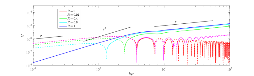
which extends Kolmogorov’s classical inertial range theory by including the forcing scale as well as bidirectional energy transfer. In contrast to the classic definition of inertial range, we do not assume that the considered scale is far away from the forcing scale , thus, (10) is a forcing-scale-resolving expression and we call it a global solution. We illustrate its behavior in Figure 1 using , , and various values of the fractional upscale flux
| (11) |
In the limit of completely upscale energy flux the present (10) reduces to the second equality in (4.9) already derived in Xie & Bühler (2018). Notably, is sign-definite and positive only if , i.e., for all values the sign of changes at least once. Also, the case with is almost indistinguishable from the limiting case for downward-only energy flux, but only if . Otherwise their difference becomes obvious as . In the intermediate range (), where is larger than the forcing scale and almost all energy transfers upscale, the structure function with still has alternating signs, which illustrates once more that one cannot safely read off the direction of the spectral transfer just from the sign of the third-order structure function.
Naturally, in the limits of large and small the global expression (10) recovers the classic local results (cf. Bernard, 1999; Lindborg, 1999; Yakhot, 1999) asymptotically, i.e.,
| (12) |
Interestingly, the small-scale “enstrophy” term recovers the classical enstrophy cascade result of 2D turbulence when , but if there may be not even be any enstrophy conservation in the turbulent system, but nonetheless this term arises in all cases in the expansion of .
2.2 Dissipative corrections
For realistic turbulence dissipation brings about corrections to (10) at large and small . E.g., in 2D turbulence a linear Ekman damping introduces the log-correlation to the energy spectrum at the enstrophy inertial range (Kraichnan, 1971), and it bounds the range of inverse energy cascade (e.g. Smith et al., 2002). We do not want to introduce a closure that links second- and third-order structure functions to calculate the shape of them, instead, we simply derive an exact relation that links them diagnostically. The derivation starts from distinguishing the large- and small-scale damping terms which dominantly absorb upscale and downscale energy fluxes, respectively. This distinction is necessary because the two types of damping influence the inertial range different in the limit of zero viscosity: the large-scale damping brings about leading-order contribution while the effect of small-scale damping is of higher order compared with that of the external forcing, as shown in Xie & Bühler (2018). Let’s write the dissipation term in (1) as
| (13) |
where the operator is the sum of large- and small-scale parts and , respectively. For example, Xie & Bühler (2018) used and for Rayleigh damping and Navier–Stokes diffusion. The large- and small-scale net dissipation rates are then and , respectively. For two-dimensional isotropic turbulence integrating (3) over a disk of radius yields
| (14) |
If the external forcing is white-noise in time and centered at wavenumber then (14) becomes
| (15) |
This is the sought-after dissipative correction to (10). We need to note that for a general 2D turbulence system we are not able to strictly derive that in the limit of zero viscosity the finite damping effect tends to zero and is therefore negligible compared with the limit result, and to do so we need to consider a specific turbulence system with prescribed damping term, one such example is 2D turbulence studied by Xie & Bühler (2018). Note that in the derivation we need to distinguish large- and small-scale dissipations. But the smallness of the finite damping effect in the zero viscosity limit matches the derivation starting from the idealized spectral energy flux (8). In the next section we check both the non-dissipative result (10) and its dissipation correction (15) in a MHD example.
3 Application to two-dimensional MHD turbulence
To test our heuristic theory we performed numerical simulations of a 2D MHD turbulent flow in which the velocity and the magnetic field are coplanar. This is an ideal test system because Seshasayana et al. (2014) found bidirectional energy transfer in this 2D system, and also its KHM equation has the generic form (1) with a third-order structure function vector (cf. Podesta, 2008) defined by
| (16) |
Here the magnetic field is normalized to have velocity units such that .
The numerical simulation uses a Fourier pseudospectral method with 2/3 dealiasing in space, a resolution and a fourth-order explicit Runge–Kutta scheme in time, in which the nonlinear terms are treated explicitly and linear terms implicitly using an integrating factor method. We take the forcing wavenumber to be , the momentum and magnetic equation are forced by random forces which are white-noise in time, and we control the kinetic energy input rate to be 100 times of that of the magnetic energy, which is a case that is found to have bidirectional energy transfer (Seshasayana & Alexakis, 2016). We add hypoviscosity with operator and hyperviscosity with operator to both the velocity and magnetic fields to dissipate energy transferred to large and small scales, respectively, and therefore the turbulence system reaches a statistically steady state.
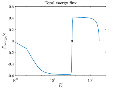
We show in the left panel of Figure 2 the spectral transfer of total energy, which is the sum of kinetic and magnetic energy. Here the spectral energy transfer is directly calculated in Fourier space from the pseudospectral code without making use of the third-order structure function in physical space. As expected, bidirectional energy transfer is observed: around of total energy transfers upscale and is mainly dissipated by the hypoviscosity, while the other transfers downscale and is mainly dissipated by the hyperviscosity; this corresponds to . In Table 1 the value of is obtained by calculating the amount of energy dissipated by the hypoviscosity and the value of is calculated from the white-noise forcing applied in the numerical simulation.
Now, the right panel of Figure 2 shows the comparison of structure functions obtained in several different ways. The blue curve shows the structure function directly measured from the statistics of the velocity and magnetic fields. The black curve is the theoretical formula (10) using the observed value of as well as the forcing wavenumber and the total energy transfer known from the numerical setup. The red curve is a least-square fitting of the theoretical result (10) using only the four measured points from the blue curve marked in green squares. We choose these four points as a test because we need to capture the sign transition of the third-order structure function and we intentionally avoid choosing points in the classic inertial ranges to distinguish our theory from the past ones: the left three points are around the region of sign change and the last point is around the forcing scale. The parameters used in the fittings are also shown in Table 1. This comparison shows that the fitting based on our global theory using only four measured structure function values works well in determining the bidirectional energy flux rate within a 5% error.
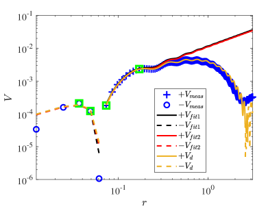
The right panel of Figure 2 also shows that the dissipation at large-scale due to hypoviscosity brings about a nonnegligible discrepancy between the theory (10) in zero-viscosity limit and the numerical data. To capture this large-scale dissipative correction we include the hypoviscosity but omit the hyperviscosity effect in (15) to obtain the viscous expression of the third-order structure function
| (17) | ||||
where and are the stream functions for and , respectively, and we have used the identity , which holds for arbitrary scalar fields with isotropic statistics. The excellent match between (17) and the numerical data verifies the validity of (15). Thus, if the damping form is known and the corresponding second-order structure function can be measured, we can make use of them to fit the data in a broader range to detect energy transfer.
4 Discussion
To test our global results (10) and (15), we deliberately used a relatively low-resolution 2D MHD simulation, which provides imperfect inertial ranges. This severely limits the applicability of classic local theories but not of the new global theory. Indeed, due to the limited resolution, the direct numerical data (blue) shows that the energy inertial ranges which have behavior are not observed. Similarly, because of the non-negligible influence from the forcing scale, a straight line corresponding to is also not clear. These make the traditional process based on classic local theories of fitting straight lines in a log-log plot to obtain the information of energy flux impossible, but our global theory can achieve it. In addition, since our global theory only contains three parameters and applies to a broader range containing forcing scale, we can make use of more data information and thereby detect the forcing scale.
The sublimits of our global expression (10) match those of the classic inertial-range results (cf. (12)) implying that our theory captures the transitions of inertial ranges. Also, it implies that simply “gluing” the theories of different inertial ranges for turbulence with unidirectional energy transfer to obtain a global theory is fallacious, because the constant in front of the depends on the total energy input instead of the upscale transferred energy alone. Also, this expansion brings about a new perspective to understanding the “enstrophy” range. In Kraichnan (1982)’s argument, the simultaneous conservation of both energy and enstrophy results in an upscale energy transfer and a downscale enstrophy transfer, and correspondingly in the enstrophy inertial range the third-order structure function has an dependence. However, our theory shows that as long as there exists nonzero upscale energy transfer, an dependence of third-order structure function exists as a natural consequence of asymptotic expansion, but the presence of a constant downscale “enstrophy” flux is not necessary with the “enstrophy” a preserved quantity without external force and dissipation, which is the case for 2D MHD turbulence.
In this paper, we present a general framework for the inertial-range third-order structure-function global theory that captures bidirectional energy transfer and resolves the forcing scale in homogeneous isotropic turbulence. This theory has three parameters, , and , that describe the upscale energy flux magnitude, downscale energy flux magnitude and the forcing scale. The classic local theories that are applicable away from the forcing scales are recovered as sublimits of this global theory, which captures the transitions as well.
In the present theory we assumed that the energy input is -centered at one wavenumber , but considering that when assuming a -centered external forcing we are solving a Green’s function for equation (3) we can express the expression of third-order structure function with a general distribution of energy input rate after a convolution. Thus, our theory can be used to detect the unknown distribution of energy input for a 2D turbulent system.
As to the finite damping effect, it is shown in Xie & Bühler (2018) that for 2D turbulence with damping operator the damping effect in (15) tends to zero as and tends to zero. But the comparable smallness of the damping effect in (15) remains to be studied carefully in other turbulence system. And it is important to justify that the different operations to the large- and small-scale damping effects is general and therefore in the limit of zero viscosity large-scale damping impacts the third-order structure function at the leading order while the influence of small-scale damping is negligible.
In the main text of this paper we only show the 2D theory for the reason that we can test it numerically. We close the paper by present the third-order structure function expression analogous to (10) for 1D (Burgers) and 3D isotropic turbulence with bidirectional energy transfer:
| (18) | ||||
| (19) | ||||
Note that the 3D result for small gives . For classic 3D turbulence, considering the relation between and the longitudinal third-order structure function
| (20) |
we recover the law of Kolmogorov (1941)’s theory: . The detailed derivations of the 1D and 3D expression are shown in §A.
We grateful to Andrew Majda and Shafer Smith for discussions that help to improve this paper. We gratefully acknowledge financial support from the United States National Science Foundation grant DMS-1312159 and Office of Naval Research grant N00014-15-1-2355.
Appendix A Derivation of the expressions of third-order structure functions in 1D and 3D
The key for deriving the expressions of third-order structure functions is obtaining the relation between structure function and energy flux, e.g. (7) in the main text, then we substitute the idealized energy flux function (cf. (8) in the main text) to obtain the final result. In this section we apply this procedure to 1D and 3D turbulence to obtain the expressions (18) and (19) in the main text.
A.1 Third-order structure function in 1D
A.2 Third-order structure function in 3D
In three dimension, the spectral energy flux (4) can be expressed as
| (S6) |
therefore under the assumption of isotropy, taking -derivative and inverse Fourier transform we obtain
| (S7) |
So we can integrate (S7) to obtain
| (S8) |
Thus, substituting the idealized expression of bidirectional energy flux (S5) into (S8) we obtain
| (22) |
which is (19).
References
- Alexakis & Biferale (2018) Alexakis, A. & Biferale, L. 2018 Cascades and transitions in turbulent flows. Phys. Rep 767–769, 1–101.
- Bernard (1999) Bernard, D. 1999 Three-point velocity correlation functions in two-dimensional forced turbulence. Phys. Rev. E 60 (5), 6184–6187.
- Cho & Lindborg (2001) Cho, J. Y. N. & Lindborg, E. 2001 Horizontal velocity structure functions in the upper troposphere and lower stratosphere 1. Observations. J. Geophys. Res. 106 (D10), 10223–10232.
- Deusebio et al. (2014) Deusebio, E., Augier, P. & Lindborg, E. 2014 Third-order structure functions in rotating and stratified turbulence: a comparison between numerical, analytical and observational results. J. Fluid Mech. 755, 294–313.
- Frisch (1995) Frisch, U. 1995 Turbulence: the legacy of A. N. Kolmogorov. Cambridge university press.
- Gallet & Doering (2015) Gallet, B. & Doering, C. R. 2015 Exact two-dimensionalization of low-magnetic-reynolds-number flows subject to a strong magnetic field. J. Fluid Mech. 773, 154–177.
- Kolmogorov (1941) Kolmogorov, A. N. 1941 Dissipation of energy in locally isotropic turbulence. In Dokl. Akad. Nauk SSSR, , vol. 32, pp. 16–18.
- Kraichnan (1971) Kraichnan, R. H. 1971 Inertial-range transfer in two- and three-dimensional turbulence. J. Fluid Mech. 47, 525–535.
- Kraichnan (1982) Kraichnan, R. H. 1982 Inertial ranges in two-dimensional turbulence. Phys. Fluids 10, 1417.
- Kurien et al. (2006) Kurien, S., L, Smith & Wingate, B. 2006 On the two-point correlation of potential vorticity in rotating and stratified turbulence. J. Fluid Mech. 555, 131–140.
- Lindborg (1999) Lindborg, E. 1999 Can the atmospheric kinetic energy spectrum be explained by two-dimensional turbulence? J. Fluid Mech. 388, 259–288.
- Lindborg (2007) Lindborg, E. 2007 Third-order structure function relations for quasi-geostrophic turbulence. J. Fluid Mech. 572, 255–260.
- Marino et al. (2015) Marino, R., Pouquet, A. & Rosenberg, D. 2015 Resolving the paradox of oceanic large-scale balance and small-scale mixing. Phys. Rev. Lett. 114, 114504.
- Monin & Yaglom (1975) Monin, A. S. & Yaglom, A. M. 1975 Statistical fluid mechanics, volume II: Mechanics of turbulence. Dover (reprinted 2007).
- Podesta (2008) Podesta, J. J. 2008 Laws for third-order moments in homogeneous anisotropic incompressible magnetohydrodynamic turbulence. J. Fluid Mech. 609, 171–194.
- Pouquet et al. (2017) Pouquet, A., Marino, R., Mininni, P. D. & Rosenberg, D. 2017 Dual constant-flux energy cascades to both large scales and small scales. Phys. Rev. Fluids 29, 111108.
- Seshasayana & Alexakis (2016) Seshasayana, K. & Alexakis, A. 2016 Critical behavior in the inverse to forward energy transition in two-dimensional magnetohydrodynamic flow. Phys. Rev. E 93, 013104.
- Seshasayana et al. (2014) Seshasayana, K., Benavides, S. Jose & Alexakis, A. 2014 On the edge of an inverse cascade. Phys. Rev. E 90, 051003(R).
- Smith et al. (2002) Smith, K. S., Boccaletti, G., Henning, C. C., Marinov, I., Tam, C. Y., Held, I. M. & Vallis, G. K. 2002 Turbulent diffusion in the geostrophic inverse cascade. J. Fluid Mech. 469, 13–48.
- Sorriso-Valvo et al. (2007) Sorriso-Valvo, L., Marino, R., Carbone, V., Noullez, A., Lepreti, F., Veltri, P., Bruno, R., Bavassano, B. & Pietropaolo, E. 2007 Observation of inertial energy cascade in interplanetary space plasma. Phys. Res. Lett. 99, 115001.
- Xie & Bühler (2018) Xie, J.-H. & Bühler, O. 2018 Exact third-order structure functions for two-dimensional turbulence. J. Fluid Mech. 851, 672–686.
- Yakhot (1999) Yakhot, V. 1999 Two-dimensional turbulence in the inverse cascade range. Phys. Rev. E 60 (5), 5544–5551.