Population synthesis of black hole binary mergers from star clusters

Abstract

Black hole (BH) binary mergers formed through dynamical interactions in dense star clusters are believed to be one of the main sources of gravitational waves for Advanced LIGO and Virgo. Here we present a fast numerical method for simulating the evolution of star clusters with BHs, including a model for the dynamical formation and merger of BH binaries. Our method is based on Hénon’s principle of balanced evolution, according to which the flow of energy within a cluster must be balanced by the energy production inside its core. Because the heat production in the core is powered by the BHs, one can then link the evolution of the cluster to the evolution of its BH population. This allows us to construct evolutionary tracks of the cluster properties including its BH population and its effect on the cluster and, at the same time, determine the merger rate of BH binaries as well as their eccentricity distributions. The model is publicly available and includes the effects of a BH mass spectrum, mass-loss due to stellar evolution, the ejection of BHs due to natal and dynamical kicks, and relativistic corrections during binary-single encounters. We validate our method using direct $N$-body simulations, and find it to be in excellent agreement with results from recent Monte Carlo models of globular clusters. This establishes our new method as a robust tool for the study of BH dynamics in star clusters and the modelling of gravitational wave sources produced in these systems. Finally, we compute the rate and eccentricity distributions of merging BH binaries for a wide range of cluster initial conditions, spanning more than two orders of magnitude in mass and radius.

1 Introduction

The advanced gravitational-wave observatories LIGO and Virgo are routinely detecting gravitational waves (GWs) from the merger of black hole (BH) binaries (Abadie et al., 2010; Acernese et al., 2015; Abbott et al., 2016b, a). The planned detector KAGRA will soon become operative (Abbott et al., 2018) and the Laser Interferometer Space Antenna (LISA), planned to launch in 2030s, will detect GWs in space (Amaro-Seoane et al., 2017), allowing to observe the BH mergers at lower frequencies and opening the doors of multi-band GW astrophysics (Sesana, 2016).

The detection of GWs has opened new perspectives for the study of compact object binaries, and has generated great interest in understanding how these sources form. A number of formation scenarios have been proposed for the formation of BH binary mergers. These include: the evolution of massive star binaries in the field of a galaxy (Belczynski et al., 2010; Dominik et al., 2012; Marchant et al., 2016; Mandel & De Mink, 2016; Gerosa et al., 2018; Michaely & Perets, 2019), the evolution of hierarchical multiple field stars (Silsbee & Tremaine, 2017; Antonini et al., 2017; Liu & Lai, 2019; Fragione & Kocsis, 2019), and dynamical few-body interactions in the core of a dense star cluster such as young star clusters (Ziosi et al., 2014; Kimpson et al., 2016b; Banerjee, 2017, 2018a, 2018b; Di Carlo et al., 2019), nuclear star clusters (Miller & Lauburg, 2009; Antonini & Rasio, 2016; Leigh et al., 2018), and globular clusters (GCs; Kulkarni et al., 1993; Sigurdsson & Hernquist, 1993; Portegies Zwart & McMillan, 2000; Downing et al., 2011; Rodriguez et al., 2015; Askar et al., 2017). In this paper we are concerned with the latter scenario, i.e. binary BH formation in star clusters of all masses.

In the dynamical formation scenario, the BH binaries are assembled through three body processes in the core of a star cluster, and subsequently harden and merge via dynamical binary-single interactions. Recent studies suggest that such binaries might account for many, or perhaps even most, binary BH mergers so far detected by LIGO-Virgo (Fragione & Kocsis, 2018; Rodriguez & Loeb, 2018; Choksi et al., 2019). Moreover, a fraction of BH binary mergers from clusters are expected to have a a finite eccentricity when they first enter the frequency band of current detectors. It has been argued therefore that GW observations of eccentric binary BH mergers will provide evidence for a dynamical formation of these systems (Antonini et al., 2014; Nishizawa et al., 2016; Breivik et al., 2016; Samsing, 2018; Rodriguez et al., 2018b). Major effort around the detection and characterisation of eccentric BH binaries is currently underway (Cao & Han, 2017; Hinder et al., 2018; Huerta et al., 2019).

Theoretical predictions for the dynamical formation channel are currently based either on Monte Carlo or direct $N$-body simulations of the long-term evolution of star clusters (Giersz, 1998; Joshi et al., 2000; Aarseth, 2012; Giersz et al., 2013). These methods allow an accurate treatment of stellar dynamical relaxation and strong encounters and have therefore the advantage that they can solve the long-term evolution of a star cluster self-consistently. Moreover, they include recipes for the effect of stellar and binary evolution, Galactic tides, primordial binaries, and relativistic corrections during strong encounters. The drawback is that the time requirements for a simulation of a realistic set of cluster models are prohibitive. For this reason, current predictions for the merger rate and source properties are based on a limited set of cluster initial conditions which do not allow to explore the relevant parameter space and uncertainties on the cluster initial conditions (e.g., Fragione & Kocsis, 2018; Rodriguez & Loeb, 2018). For example, Fragione & Kocsis (2018) ignored the dependence of the binary merger rate on the cluster initial radius and its evolution. Rodriguez & Loeb (2018) derived their binary BH merger rate assuming that $50\%$ of clusters form with a virial radius of $r_{\rm v}=1\,$pc and the rest with $2\,$pc. To fully explore the parameter space that controls dynamically formed BH mergers, a significantly faster recipe is required, without giving in too much on the accuracy of the obtained results.

In this paper we present a new, fast computational method for the evolution of a star cluster with BHs, including a prescription for the dynamical evolution of the BH binaries. Any of our model takes less than a second to complete (using a commercial laptop). In comparison, the typical wall-clock computation time for a full $N$-body model of $\sim 10^{6}~{}{\rm M}_{\odot}$ cluster is about a year on a super-computer with Graphical Processing Units (GPUs, Wang et al., 2016), and a similar Monte Carlo cluster model will require about one week on a standard multi-core PC.

Our method relies on Hénon’s principle (Hénon, 1975), which states that after an initial settling phase the rate of heat generation in the core is a constant fraction of the total cluster energy per half-mass relaxation time. Breen & Heggie (2013) showed that in this so-called ‘balanced evolution’ phase the heat is produced by the BHs, and one can therefore link the evolution of the BH population to the properties of the cluster itself. This allows us to construct a series of coupled first-order differential equations to express the time evolution of a cluster mass, radius, and the total mass in BHs. We further assume that during binary-single interactions the eccentricity of the BH binaries follows that of a so-called thermal distribution $N(e)\propto e$ (e.g., Heggie, 1975). Based on this assumption, we derive the merger rate, and the eccentricity distribution of the BH binaries and their relation to a cluster global properties.

The paper is organised as follows. In Section 2 we present the model for the co-evolution of a BH population and its host cluster, and use direct $N$-body simulations to validate this simple model. Section 3 describes the analytical prescriptions to determine the rate and eccentricity distributions of BH binary mergers formed via binary-single interactions. In Section 4 we compare the results of our model to those of independent Monte Carlo simulations from published literature. Finally, in Section 5 we make predictions for the merger rate and eccentricities of BH binaries for a wide range of cluster initial conditions, and discuss how these distributions are linked to a cluster properties.

2 Evolution of star clusters with a black hole population

2.1 Philosophy of the model

In this section we present a fast model for the co-evolution of a BH population and its host cluster. To achieve speed, we only evolve several bulk properties of the cluster and not its internal structure. We limit the model to the cluster properties that are most relevant for the formation and evolution of binary BHs. The hard-soft boundary of binaries is set by the velocity dispersion of the cluster, which is proportional to $\sqrt{M_{\rm cl}/r_{\rm h}}$, where $M_{\rm cl}$ is the total cluster mass and $r_{\rm h}$ its half-mass radius. The binding energy, and therefore, the semi-major axis of escaping BH binaries depends on the central escape velocity ($v_{\rm esc}$) of the cluster (see Rodriguez et al. 2016), which is also proportional to $\sqrt{M_{\rm cl}/r_{\rm h}}$. The condition for in-cluster BH binary mergers to be efficient can also be expressed in $M_{\rm cl}$ and $r_{\rm h}$ (see Antonini et al. 2019). We therefore model the evolution of $M_{\rm cl}$ and $r_{\rm h}$. We will solve differential equations for $\dot{M}_{\rm cl}$ and $\dot{r}_{\rm h}$, as is done in the fast cluster evolution model emacss (Alexander & Gieles, 2012; Gieles et al., 2014; Alexander et al., 2014). Here we add the evolution of the BH population, and its effect on the evolution of the cluster. We approximate the cluster by a two component system: a light component, consisting of the stars, white dwarfs and neutron stars, and a heavy component of BHs.

Breen & Heggie (2013) showed that once a star cluster achieves the balanced evolution phase, the total mass of the BH population in a cluster ($M_{\rm BH}$) depends on $M_{\rm cl}$ and the half-mass relaxation time-scale ($t_{\rm rh}$) of the cluster as $\dot{M}_{\rm BH}\propto M_{\rm cl}/t_{\rm rh}$. This dependence of $M_{\rm BH}$ on the cluster properties, rather than the properties of the core where the BH binaries reside, is because the heat production in the core is set by the properties of a cluster as a whole (Hénon, 1961), and the BH binaries provide the heat via dynamical interactions with other BHs, resulting in ejections of BHs and binaries (more on this in Section 2.3). This discovery by Breen & Heggie allows us to relate the evolution of the BH population to the cluster properties and we therefore jointly solve for $M_{\rm cl}$, $r_{\rm h}$ and $M_{\rm BH}$ from the expressions for their time derivatives.

We restrict ourselves in this paper to isolated star clusters, avoiding the complication of the Galactic tidal field. This will result in unrealistic cluster properties at redshift $z\simeq 0$ for clusters that are strongly tidally limited, but most of the BH binaries that are relevant for GW detections are produced at high $z$, when the clusters are dense compared to the tidal density (Gieles et al., 2010), and then GC evolution is comparable to that of isolated GCs (Gieles, Heggie & Zhao, 2011). Clusters with low densities are more affected by the tides, but less relevant for GWs. In addition, the most massive GCs, which are most important for GW production (Antonini & Rasio, 2016) are still largely unaffected by the tidal field at $z=0$ (Gieles et al., 2011), providing further support for our assumption.

We first present in Section 2.2 a prescription for the fraction of the initial $M_{\rm BH}$ that is retained after natal kicks and in Section 2.3 we discuss the co-evolution of $M$, $r_{\rm h}$ and $M_{\rm BH}$. In Section 2.4 we compare the model to a series of direct $N$-body simulations and use these to determine a few model parameters.

2.2 Retention after supernova kicks

For the initial conditions we need $M$, $r_{\rm h}$ and $M_{\rm BH}$ at $t=0$, i.e. when the cluster forms. The value of $M_{\rm BH}$ is zero initially, because all stars are on the main sequence, but for simplicity we assume that all BHs are already in place at formation avoiding the need for describing BH formation in the first $\sim 20~{}$Myr. The initial value of $M_{\rm BH}$ then depends on the stellar initial mass function (IMF) and the initial-final mass relation (IFMR), which depends on metallicity ([Fe/H]). At lower [Fe/H], BHs are more massive (e.g. Spera et al., 2015) such that – for a given IMF – $M_{\rm BH}$ is larger. The [Fe/H] and IMF dependence can be parameterised. Here, we focus on a canonical Kroupa et al. (2001) IMF, for which a fraction $f_{0}\simeq 0.06$ of the initial $M_{\rm cl}$ ends up in BHs for metal-poor GCs.

Because BHs receive natal kicks, and the condition for escape depends on $v_{\rm esc}$, we need a relation for the retention of the mass retention fraction after supernova (SN) kicks ($f_{\rm ret}^{M}$). Although the magnitude of BH natal kick velocity ($v_{\rm kick}$) is not known, there is some consensus that BH kicks are smaller than those of neutron stars (Mandel, 2016), and it likely depends on the mass of the BH ($m$), with the more massive BHs receiving smaller kicks. If the escape velocity from the centre of the cluster ($v_{\rm esc}$), where most BHs are expected to form, is much larger than $v_{\rm kick}$ of the lowest mass BH, then $f_{\rm ret}^{M}\simeq 1$. If $v_{\rm esc}$ is much smaller than $v_{\rm kick}$ of the most massive BHs, then $f_{\rm ret}^{M}\simeq 0$. In the GC-mass range, $v_{\rm esc}$ is likely to be in the intermediate regime, and for a given BH mass $m$, there is then a distribution of $v_{\rm kick}$ values. Both of these effects need to be captured by our expression for $f_{\rm ret}^{M}(v_{\rm esc})$.

To proceed, we assume that $v_{\rm kick}$ is drawn from a Maxwell-Boltzmann distribution, $P_{\rm B}(v_{\rm kick}|\sigma_{\rm k})$, with dispersion $\sigma_{\rm k}$. We then assume that BHs receive the same momentum kick as neutron stars (Fryer & Kalogera, 2001), such that $\sigma_{\rm k}(m)=\sigma_{\rm NS}\times m_{\rm NS}/m$, for which we adopt $\sigma_{\rm NS}=265\,{\rm km\,s}^{-1}$ is the dispersion for neutron star kicks (Hobbs et al., 2005) and $m_{\rm NS}=1.4~{}{\rm M}_{\odot}$ is the mass of a neutron star. The resulting kicks are smaller than in the fallback scenario (Dominik et al., 2013), but for our simple model the assumption of a constant momentum kick is preferred, because it allows us to derive a simple expression for $f_{\rm ret}^{M}(v_{\rm esc})$, without detailed knowledge of the fallback fraction of BHs with different masses. We ignore direct collapse SNe in this version of the model, but note that more detailed kick prescriptions will be considered in future versions of the model.

The retained number fraction of BHs with mass $m$ is then given by the integral over $P_{\rm B}$ from zero to $v_{\rm esc}$

$$f_{\rm ret}^{N}(v_{\rm esc},m)=\int_{0}^{v_{\rm esc}}P_{\rm B}(v^{\prime}|\sigma_{\rm k}){\rm d}v^{\prime}=C_{\rm B}(v_{\rm esc}|\sigma_{\rm k}),$$ (1)

where $C_{\rm B}(v_{\rm esc}|\sigma_{\rm k})$ is the cumulative distribution function of the Maxwell-Boltzmann distribution.

To find $f_{\rm ret}^{M}$, we define the BH mass function after SN kicks, $\phi(m)$, defined as the number of BHs in an interval $(m,m+{\rm d}m)$. This mass function follows from the birth BH mass function, $\phi_{0}(m)$, as

$$\phi(v_{\rm esc},m) =C_{\rm B}(v_{\rm esc}|\sigma_{\rm k})\phi_{0}(m),$$ (2)

$$\simeq\frac{\phi_{0}(m)}{(m_{\rm b}/m)^{3}+1}.$$ (3)

In the last step we used an approximation, where $m_{\rm b}=(9\pi/2)^{1/6}\sigma_{\rm NS}m_{\rm NS}/v_{\rm esc}$ is the mass below which the BH mass function is affected by kicks. For all $\phi_{0}$, this approximation underestimates the exact result by only $\sim 10\%$ at $m\simeq m_{\rm b}$, and quickly approaches to the exact result for other values of $m$. This simple approximation for $\phi$ serves to derive the maximum BH mass from $M_{\rm BH}$ when we include escape of BHs.

The mass retention fraction $f_{\rm ret}^{M}$ is then found from integrating $\phi$ over all BH masses,

$$f_{\rm ret}^{M}(v_{\rm esc})=\int_{m_{\rm lo}}^{m_{\rm up}}\phi(m)m{\rm d}m\bigg{/}\int_{m_{\rm lo}}^{m_{\rm up}}\phi_{0}(m)m{\rm d}m\ .$$ (4)

Assuming a power-law $\phi_{0}\propto m^{\alpha}$ and the approximation for $\phi$ from equation (3), then equation (4) gives

$$f_{\rm ret}^{M}(v_{\rm esc}) \simeq\int_{m_{\rm lo}}^{m_{\rm up}}\frac{m^{\alpha+1}}{(m_{\rm b}/m)^{3}+1}{\rm d}m\bigg{/}\int_{m_{\rm lo}}^{m_{\rm up}}m^{\alpha+1}{\rm d}m$$

$$=\begin{cases}\displaystyle\ln{\left[\left(q_{\rm ub}^{3}+1\right)/\left(q_{\rm lb}^{3}+1\right)\right]}/\ln\left(q_{\rm ul}^{3}\right),&\alpha=-2,\vspace{0.2cm}\\ \displaystyle 1-\left[q_{\rm ul}^{\alpha+2}h(q_{\rm ub})-h(q_{\rm lb})\right]/\left(q_{\rm ul}^{\alpha+2}-1\right),&\alpha\neq-2,\end{cases}$$ (5)

Here $m_{\rm lo}$ and $m_{\rm up}$ are the lower and upper limit of $\phi_{0}$, respectively, and $q_{\rm ul}=m_{\rm up}/m_{\rm lo}$, $q_{\rm ub}=m_{\rm up}/m_{\rm b}$, $q_{\rm lb}=m_{\rm lo}/m_{\rm b}$ and $h(x)={{}_{2}}F_{1}\left(1,(\alpha+2)/3;(\alpha+5)/3;-x^{3}\right)$, with ${{}_{2}}F_{1}\left(a,b;c;x\right)$ a hypergeometric function. This function diverges for negative integer values of $c$ and for $c=0$, hence the result for $f_{\rm ret}^{M}$ in equation (5) for $\alpha\neq-2$ also excludes the values $\alpha=-5,-8,-11,\dots$, but because such steep mass functions are not expected for BHs, we refrain from giving the full solution for those values. In Fig. 1 we show results obtained from numerical integrations of equation (2) in thick lines, and the approximation of equation (5) with thin lines. We assumed a power-law $\phi_{0}$, adopting both a declined and a rising BH mass function ($\alpha=-1$ and $\alpha=+1$, respectively), between $m_{\rm lo}=3~{}{\rm M}_{\odot}$ and $m_{\rm up}$, for which we used $m_{\rm up}=25~{}{\rm M}_{\odot}$ and $m_{\rm up}=35~{}{\rm M}_{\odot}$. From Fig. 1 we see that at low $v_{\rm esc}$, the retention fraction can be well approximated by $f_{\rm ret}^{M}\propto v_{\rm esc}^{3}$, which is the leading order term of $C_{\rm B}(v_{\rm esc}|\sigma_{\rm k})$. More specifically we find

$$f_{\rm ret}^{M}(v_{\rm esc})\propto\frac{v_{\rm esc}^{3}}{\sigma_{\rm NS}^{3}}\frac{\langle m^{4}\rangle}{\langle m\rangle}.$$ (6)

This shows that at low $v_{\rm esc}$, $f_{\rm ret}^{M}$ depends on the cluster properties as $v_{\rm esc}^{3}\propto(M/r_{\rm h})^{3/2}$ and is sensitive to the most massive BH, because for top-heavy $\phi$ (i.e. $\alpha>-2$) and $m_{\rm up}>>m_{\rm lo}$ we find $\langle m^{4}\rangle/\langle m\rangle\propto m_{\rm up}^{3}$. This sensitivity to $m_{\rm up}$ implies that for a given $v_{\rm esc}$, $f_{\rm ret}^{M}$ is higher in low-metallicity GCs, for which BHs are more massive. This statement is valid for a continuous $\phi$, since $f_{\rm ret}^{M}$ can be low if – for example – a single, massive BH forms among a population of low-mass BHs.

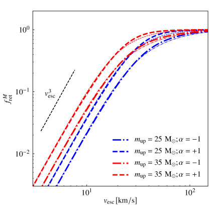
Figure 1: Fraction of BH mass retained after SNe as a function of $v_{\rm esc}$. The thick (blue and red) lines show results from equation (2), for different $m_{\rm up}$ and BH mass function slope $\alpha$. The thin lines show the approximation from equation (5).

2.3 Co-evolution of the cluster and its BH population

In this section we present a model for the temporal evolution of $M_{\rm cl}$, $r_{\rm h}$ and $M_{\rm BH}$. We consider clusters in isolation, which lose mass by stellar evolution and BHs via dynamical interactions. We define expressions for $\dot{M}_{\rm cl}$, $\dot{r}_{\rm h}$ and $\dot{M}_{\rm BH}$, which are then integrated numerically.

2.3.1 Stellar mass loss

We assume that the cluster consists of two types of members: BHs and all the other members (i.e. other stellar remnants and stars). Each contribute a mass of $M_{\rm BH}$ and $M_{\star}$, respectively, such that $M_{\rm cl}=M_{\star}+M_{\rm BH}$. We assume that as a result of stellar mass loss, $M_{\star}$ evolves as a power of time, such that

$$\dot{M}_{\star,\rm sev}=\begin{cases}0,&t<t_{\rm sev},\\ \displaystyle-\nu{M_{\star}\over t},&t\geq t_{\rm sev},\end{cases}$$ (7)

with $t_{\rm sev}\simeq 2\,\rm Myr$ and $\nu\simeq 0.07$, depending slightly on [Fe/H]. We further assume that as a result of stellar mass loss the cluster expands adiabatically, such that

$$\dot{r}_{\rm h,sev}=-{\dot{M}_{\star,\rm sev}\over M_{\rm cl}}r_{\rm h}.$$ (8)

Note that we here assumed that stellar mass-loss occurs throughout the cluster, and the expansion rate could be higher if the cluster is mass segregated and mass loss occurs more central. This can be included (see Alexander et al., 2014), but here we do not implement this, because in the presence of BHs and for high density clusters, the evolution becomes quickly dominated by relaxation driven expansion, as we will show in the next section.

2.3.2 Relaxation

After several relaxation time-scales have elapsed, the core of the cluster starts producing energy in order to sustain the relaxation process. We define the start of this balanced evolution as

$$t_{\rm cc}=N_{\rm rh}t_{\rm rh,0},$$ (9)

where $N_{\rm rh}$ is a constant of order unity that we will fit to $N$-body models in Section 2.4 and $t_{\rm rh,0}$ is the initial half-mass relaxation time-scale. It would be more accurate to express $t_{\rm cc}$ in terms of the number of elapsed relaxation time-scales (Alexander et al., 2014), but for simplicity we here express $t_{\rm cc}$ in the timescale that can be straightforwardly evaluated at the start of the model computation. The start of balanced evolution corresponds to the collapse of the core, which is dominated by BHs in case $f_{\rm ret}^{M}>0$. This type of core collapse occurs well before the collapse of the core of visible stars, which coincides with the moment that all BHs are ejected (Breen & Heggie, 2013).

The half-mass relaxation time-scale is the average relaxation time-scale within $r_{\rm h}$, which is given by (Spitzer & Hart, 1971)

$$t_{\rm rh}=0.138\sqrt{\frac{M_{\rm cl}r_{\rm h}^{3}}{G}}\frac{1}{\langle m_{\rm all}\rangle\psi\ln\Lambda}.$$ (10)

Here $\langle m_{\rm all}\rangle$ is the mean mass of the stars and all stellar remnants, which we initially set to $\langle m_{\rm all}\rangle=\langle m_{\star}\rangle\simeq 0.638\,{\rm M}_{\odot}$, which is found for a Kroupa et al. (2001) IMF between 0.1 and $100~{}{\rm M}_{\odot}$. During the evolution $\langle m_{\rm all}\rangle=M_{\rm cl}/N_{\rm cl}$, where $N_{\rm cl}$ is the initial number of stars which we assume to be constant throughout the evolution, which is accurate in the case of 100% BH retention and no pair-instability SNe, and slightly overestimates the number of stars once BH ejection occurs and at later times when the turn-off mass drops. Then, $\ln\Lambda$ is the Coulomb logarithm, which depends weakly on $N_{\rm cl}$, and we therefore use a constant $\ln\Lambda=10$.

The quantity $\psi$ depends on the mass spectrum within $r_{\rm h}$, which is usually assumed to be $\psi=1$, applicable to systems of equal mass but in reality $\psi$ can be between $1.5-2$ for GC like mass functions (Spitzer & Hart, 1971; Kim et al., 1998) and $30-100$ for clusters that just formed (Gieles et al., 2010). In emacss, a time-dependent $\psi$ was adopted to include the effect of the loss of massive stars by stellar evolution on the relaxation process. However, emacss was compared to $N$-body models without BHs (Baumgardt & Makino, 2003) and here we want to include the effect of BHs on $\psi$. We therefore search for an expression with a dependence on the properties of the BH population.

Spitzer & Hart (1971) derive an expression for $\psi$ for multi-component systems, under the assumption of equipartition (their equation 24): $\psi=\langle m_{\rm all}^{5/2}\rangle/\langle m_{\rm all}\rangle^{5/2}$. For our two components model this can be written as: $\psi=(m_{\star}^{3/2}M_{\star}+m^{3/2}M_{\rm BH})N_{\rm cl}^{3/2}/M_{\rm cl}^{5/2}$. For $M_{\star}\simeq M_{\rm cl}$ and $m>>m_{\star}$ (such that also the number of BHs is small), this expression for $\psi$ reduces to

$$\psi\simeq 1+\frac{M_{\rm BH}}{M_{\star}}\left(\frac{m}{m_{\star}}\right)^{3/2}.$$ (11)

The second term on the right-hand side is Spitzer’s parameter $S$ (Spitzer, 1969), whose value determines whether a system can achieve equipartition ($S\leq 0.16$). For $M_{\rm BH}/M_{\star}=0.05$ and $m/m_{\star}\simeq 20$ (see e.g. Zocchi et al., 2019, for the case of $\omega$ Cen), we find $S\simeq 4$. This is larger than the criteria for a two-component system to achieve equipartition. Clusters with such a BH population are therefore not expected to achieve equipartition in the centre (see also Peuten et al., 2017, who show this with $N$-body simulations of star clusters with BHs). If we instead of equipartition assume that all members have the same velocity dispersion, then $\psi\simeq 1+(M_{\rm BH}/M_{\star})(m/m_{\star})$, i.e. the index $3/2$ in equation (11) reduces to 1. An additional complexity is that the values of $M_{\rm BH}$ and $M_{\star}$ in equation (11) apply to the conditions within $r_{\rm h}$, where BHs are contributing more to the mass than for the cluster as a whole.

We therefore adopt a functional form inspired by equation (11) and introduce a free parameter

$$\psi=1+a_{1}{f_{\rm BH}\over 0.01},$$ (12)

where $f_{\rm BH}=M_{\rm BH}/M_{\rm cl}$ is the fraction of the total cluster mass that is in BHs. With this expression, we have included the dynamical feedback from the BHs on the relaxation process of the cluster. In Section 2.4 we show that the evolution of a cluster can be well described by a constant $a_{1}$ of order unity and that it is important to include this dependence of $\psi$ on $f_{\rm BH}$ , as for $f_{\rm BH}\simeq 0.05$ and $a_{1}\simeq 1$, we find $\psi\simeq 6$, which has a significant effect on the relaxation process. Clearly, relaxation is more important in the early stages when $\psi$ is large, while $\psi$ decreases in time because of the ejection of BHs, narrowing the mass spectrum. We note that $a_{1}$ could then also become smaller, because $m/m_{\star}$ decreases as the most massive BHs are ejected first, but in this first version of the model we continue with the simple linear dependence of $\psi$ on $f_{\rm BH}$ (i.e. equation 12) and reserve a dependence on the BH mass function for future improvements.

In clusters with BHs, the heating in the balanced evolution phase is done by the BHs (Breen & Heggie, 2011), in the form of a BH binary that heats the surrounding BHs, which in turn efficiently transfer the heat to the stars because of the large mass ratio $m/m_{\star}$. The dynamical hardening of BH binaries is an energy source which complies with Hénon’s principle (Hénon, 1975). In this, the rate of energy generation in the core is set by the maximum heat flow that can be conduced from the core to the rest of the cluster through two-body relaxation, and we can therefore relate the heat generation in the core to the cluster global properties (Hénon, 1961; Gieles et al., 2011; Breen & Heggie, 2013)

$$\dot{E}=\zeta\frac{|E|}{t_{\rm rh}},$$ (13)

where $E\simeq-0.2GM_{\rm cl}^{2}/r_{\rm h}$ is the total energy of the cluster, with the constant $\zeta\simeq 0.1$ (Hénon, 1961; Gieles et al., 2011; Alexander & Gieles, 2012). This definition of the energy excludes the (negative) energy stored in binaries and this energy is therefore sometimes referred to as the ‘external energy’ (Heggie & Aarseth, 1992; Giersz & Heggie, 1997). If heating is done by binaries and in the absence of other changes to $E$ (e.g. stellar evolution, Galactic tides, etc.), negative energy flows into binaries in the centre at a rate $-\dot{E}$, while $E$ increases at a rate $+\dot{E}$ (equation (13). As a result, the cluster expands and loses mass via BH escapers from the core, see e.g. Goodman (1984). Note that the efficiency of heat conduction within the cluster is included in $t_{\rm rh}$ via $\psi$, in the sense that $\dot{E}$ is higher in clusters with high $f_{\rm BH}$.

Breen & Heggie (2013) showed that BHs power the relaxation process, and using theory and $N$-body simulations they showed that this implies that the mass evolution of the BH population can be coupled to the properties of the cluster. The explanation for this is, in short, as follows: a BH binary hardens until it ejects itself as the result of the recoil in the last encounter. If all BHs have the same mass, the BH binary ejects on average $\sim 4$ BHs before ejecting itself (see Goodman, 1984). This allows us to couple the mass-loss rate of BHs to the energy generation rate, which itself is coupled to the total $E$ and $t_{\rm rh}$ of the cluster (equation 13), such that (Breen & Heggie, 2013)

$$\dot{M}_{\rm BH}=\begin{cases}0,&t<t_{\rm cc}{\rm~{}or~{}}M_{\rm BH}=0,\\ \displaystyle-\beta{M_{\rm cl}\over t_{\rm rh}}\ ,&t\geq t_{\rm cc}{\rm~{}and~{}}M_{\rm BH}>0.\end{cases}$$ (14)

From the definition of $E$ (given just under equatioin 13) and the assumption of virial equilibrium we find that $\dot{E}/|E|=-2\dot{M}_{\rm cl}/M_{\rm cl}+\dot{r}_{\rm h}/r_{\rm h}$, such that the expansion rate as the result of relaxation is

$$\dot{r}_{\rm h,rlx}=\zeta{r_{\rm h}\over t_{\rm rh}}+2\frac{\dot{M}_{\rm cl}}{M_{\rm cl}}r_{\rm h}\ .$$ (15)

Both stellar mass loss and BH ejection contribute to the mass loss of the cluster, such that

$$\dot{M}_{\rm cl}=\dot{M}_{\star,\rm sev}+\dot{M}_{\rm BH}\ .$$ (16)

Quantifying the interplay between these two mass-loss terms on the energy evolution is beyond the scope of this work, and we simply quantify the rate of BH ejection by fitting $\beta$ to the $N$-body models.

The final expression for the half-mass radius evolution is then

$$\dot{r}_{\rm h}=\begin{cases}\dot{r}_{\rm h,sev},&t<t_{\rm cc},\\ \dot{r}_{\rm h,sev}+\dot{r}_{\rm h,rlx},&t\geq t_{\rm cc}.\end{cases}$$ (17)

With all the expressions for the derivatives, we can now numerically solve a set of coupled ordinary differential equations to obtain solutions for $M_{\star}(t),M_{\rm BH}(t)$ (and therefore $M_{\rm cl}(t)$) and $r_{\rm h}(t)$.

We fix the parameters $t_{\rm sev}=2\,{\rm Myr}$, $\zeta=0.1$ and determine $N_{\rm rh}$, $\beta$, $\nu$ and $a_{1}$ by fitting the model of this section to results of direct $N$-body simulations.

2.4 Comparison to $N$-body simulations

To validate the simple model, we simulate the evolution of clusters with BHs with direct $N$-body simulations, with different initial cluster densities and BH natal kicks. For the calculations we use nbody6 (version downloaded on 25 May 2016), which is a fourth-order Hermite integrator with an Ahmad & Cohen (1973) neighbour scheme (Makino & Aarseth, 1992; Aarseth, 1999, 2003), and force calculations that are accelerated by Graphics Processing Units (GPUs, Nitadori & Aarseth, 2012). nbody6 contains metallicity dependent prescriptions for the evolution of individual stars and binary stars (Hurley et al., 2000, 2002b).

We model 4 different initial densities within $r_{\rm h}$: $\rho_{\rm h}=[10^{1},10^{2},10^{3},10^{4}]\,{\rm M}_{\odot}/{\rm pc}^{3}$, with the initial positions and velocities drawn from a Plummer (1911) model. For each density we consider two assumptions for the BH kicks: (1) no kicks and (2) kicks with the same momentum as neutron stars. In the latter, $v_{\rm kick}$ is drawn from a Maxwell-Boltzmann distribution with $\sigma_{\rm k}=\sigma_{\rm NS}\times 1.4\,{\rm M}_{\odot}/m$, and $\sigma_{\rm NS}=190\,{\rm km\,s}^{-1}$. For $v_{\rm esc}$ we use equation (29), with $f_{c}=0.68$, applicable to the average escape velocity of stars in a Plummer model. We use a metallicity of $Z=0.0006$ (i.e. ${\rm[Fe/H]}\simeq-1.5$), typical for metal-poor GCs in the Milky Way and all clusters have $N=10^{5}$ stars initially, drawn from a Kroupa et al. (2001) IMF between 0.1 and 100 ${\rm M}_{\odot}$, such that initially $\langle m_{\star}\rangle=0.638\,{\rm M}_{\odot}$. For these parameters the maximum $m\simeq 28~{}{\rm M}_{\odot}$. This is lower than what is found from more recent IFMRs that have been implemented in nbody6 (Banerjee et al., 2019), but for the purpose of our model testing this is no concern. In future versions of our model clusterBH we will compare to a range of [Fe/H] and IFMRs. All models are evolved until 11.5 Gyr.

To determine the posteriors of the clusterBH parameters, we determine the values of $M_{\rm cl}$, $M_{\rm BH}$ and $r_{\rm h}$ from the $N$-body models at 200 equally spaced time intervals between 10 Myr and 11.5 Gyr. We then define a log-likelihood

$$\ln\mathcal{L}=-\sum_{k=1}^{8}\sum_{j=1}^{3}\sum_{i=1}^{200}\frac{(D_{ijk}-M_{ijk})^{2}}{(\delta D_{ijk})^{2}},$$ (18)

where $D_{ijk}$ is a $8\times 3\times 200$ array with the $N$-body data of the simulations, and $M_{ijk}$ is a similar sized array with the clusterBH results. The index $k$ loops over the 8 $N$-body models, the index $j$ over the 3 physical quantities ($M_{\star},r_{\rm h},M_{\rm BH}$) and the index $i$ over 200 equally spaced time steps in the range 10 Myr - 11.5 Gyr. We assume each $N$-body data value has an associated uncertainty $\delta D_{ijk}=0.05D_{ijk}$, which captures the fact that cluster parameters evolve with some noise in time and cluster-to-cluster variation.

The parameters that maximise this log-likelihood are found with emcee (Foreman-Mackey et al., 2013), which is a pure-python implementation of the Goodman & Weare’s affine invariant Monte Carlo Markov Chain (MCMC) ensemble sampler (Goodman & Weare, 2010). We use 100 walkers and after a few hundred steps the fit converged. We continued for 1000 steps and in the analyses we use the final walker positions to generate posterior distributions. The python implementation of emcee makes it straightforward to couple it to clusterBH.

For the parameters we find $N_{\rm rh}=3.21$, $\beta=2.80\times 10^{-3}$, $\nu=8.23\times 10^{-2}$ and $a_{1}=1.47$. Because the uncertainties on the $N$-body data are artificial, we do not report the uncertainties in the parameters. Instead, we compute for each $N$-body data point the fractional difference with the best-fit model and sort all values. We find that 68% of the $N$-body data points are reproduced within 12.8%. Given the simplicity of our model, we consider this accuracy satisfactory. The clusterBH results are shown in Fig. 2 and Fig. 3 for 100% BH retention and for momentum conserving BH kicks, respectively. We note that when fitting the model to individual models, better agreement can be obtained, but we are here aiming to obtain model parameters that describe the evolution of all 8 $N$-body models. We note that clusterBH slightly over-predicts rate of BH escape for low $M_{\rm BH}$ (see bottom panels of Fig. 3), which is likely the result of that fact that we did not include a dependence on $m/m_{\star}$ in $\psi$ (equation 12). Including this would reduce $|\dot{M}_{\rm BH}|$ because when the BH population is about the disappear, the average BH masses are lower than in the early evolution. The good resemblance between the overall evolution of all parameters in the 8 models between the detailed $N$-body models and clusterBH confirms that the model does a good job.

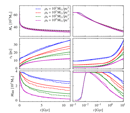
Figure 2: $N$-body results of $M_{\star}$ (top), $r_{\rm h}$ (middle) and $M_{\rm BH}$ (bottom) of isolated star clusters with 100% BH retention for different initial densities (dashed lines). Best-fit clusterBH models are shown as full-lines.

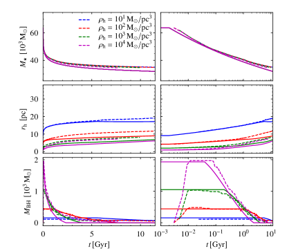
Figure 3: $N$-body results of $M_{\star}$ (top), $r_{\rm h}$ (middle) and $M_{\rm BH}$ (bottom) of isolated star clusters with different initial densities with BH kicks applied (dashed lines). Best-fit clusterBH models are shown as full-lines.

3 Black hole binary evolution

According to Hénon’s principle the flow of energy through the half-mass radius is independent of the precise mechanisms for energy production within the core. We assume in what follows that the heat is supplied by the hard binaries in the core of the BH subsystem (e.g., Breen & Heggie, 2013). Assuming that most of the heating is produced by one binary in the core of the star cluster, we can then relate the binary hardening rate to the rate of energy generation

$$\dot{E}_{\rm bin}={\dot{E}}\ .$$ (19)

where $E_{\rm bin}=Gm_{1}m_{2}/2a$, with $a$ the binary semi-major axis and $m_{1}$ and $m_{2}$ the mass of the BH components. In this section we use equation (19) to derive the merger rate and eccentricity distributions of merging BH binaries produced through binary-single interactions. To achieve this, we first need to specify the dynamical mechanisms that lead to the mergers.

The merger of a BH binary through (strong) binary-single encounters in a dense star cluster following its formation and dynamical hardening can occur in three different ways (e.g., Gültekin et al., 2006; Rodriguez et al., 2018b; Samsing, 2018): (i) the merger occurs in between binary-single encounters while the binary is still bound to its parent cluster (hereafter, we will refer to these mergers as in-cluster inspirals); (ii) a merger occurs during a binary-single (resonant) encounter as two BHs are driven to a short separation such that GW radiation will lead to their merger before the next intermediate binary-single state is formed (hereafter, GW captures); and (iii) the binary merges after it has been ejected from its parent cluster. In what follows we derive an analytical model, BHBdynamics, to compute the rate and eccentricity distributions of merging BH binaries that are produced through the mechanisms (i), (ii) and (iii). This model can then be easily coupled to clusterBH in order to compute such distributions for and evolving model of a star cluster (Section 5). Hereafter, the combination of our two models is referred to as clusterBHBdynamics.

3.1 Merger fractions

3.1.1 In-cluster inspirals.

The binary-single interactions in the cluster core lead to a decrease in the binary semi-major axis until the binary evolution becomes dominated by GW energy loss. The timescale, $t_{3}$, over which a binary will encounter another BH in the cluster core can be obtained by noting that binaries release on average 20% of their binding energy to the passing BH in an encounter, such that $\dot{E}_{\rm bin}\simeq 0.2{E}_{\rm bin}/t_{3}$ (Heggie & Hut, 2003), which leads to the relation

$$t_{3}\simeq 0.2{Gm_{1}m_{2}\over 2a}\dot{E}_{\rm bin}^{-1}\ .$$ (20)

At later times, the evolution of the binary semi-major axis and eccentricity is described by the orbit averaged evolution equations (Peters, 1964):

$$\dot{a}_{\rm GW}=-{64\over 5}\frac{G^{3}m_{1}m_{2}m_{12}}{c^{5}a^{3}\ell^{7}}\left(1+{73\over 24}e^{2}+\frac{37}{96}e^{4}\right)\$$ (21)

$$\dot{e}_{\rm GW}=-{304\over 15}{G^{3}m_{1}m_{2}m_{12}\over c^{5}a^{4}\ell^{5}}\left(e+{121\over 304}e^{3}\right)\ ,$$ (22)

with $\ell\equiv(1-e^{2})^{1/2}$ the dimensionless angular momentum, $e$ the binary eccentricity, and $m_{12}=m_{1}+m_{2}$. We define the corresponding merger timescale as $t_{\rm GW}\equiv a/\left|\dot{a}_{\rm GW}\right|$.

The transition from the dynamical to the GW regimes occurs at $t_{\rm GW}\lesssim t_{3}$, or equivalently when for a given $a$ the eccentricity is larger than

$$\ell<\ell_{\rm GW}\simeq 1.3\left[{G^{4}\left(m_{1}m_{2}\right)^{2}m_{12}\over c^{5}\dot{E}_{\rm bin}}\right]^{1/7}a^{-5/7}\ ,$$ (23)

where $\dot{E}_{\rm bin}$ is related to the properties of the cluster through equation (13), and we have taken the relevant limit $e\rightarrow 1$. For $\ell\lesssim\ell_{\rm GW}$ the evolution becomes dominated by GW energy loss and the binary inspirals approximately as an isolated system.

During a single interaction with a cluster member of mass $m_{3}$ the semi-major axis of the binary decreases from $a$ to $\epsilon a$. Then energy and momentum conservation imply that the binary will experience a recoil kick $v_{\rm bin}^{2}\simeq G\mu{m_{3}\over{m_{123}}}\left[1/(\epsilon a)-1/a\right]=\left(1/\epsilon-1\right)G{m_{1}m_{2}\over m_{123}}{q_{3}/a}$, where $\mu=m_{1}m_{2}/m_{12}$, $m_{123}=m_{12}+m_{3}$, $q_{3}=m_{3}/m_{12}$, and we have assumed that in the interaction the binding energy of the binary increases by the fixed fraction $\left(1/\epsilon-1\right)=0.2$, which implies $\epsilon=0.83$ (e.g., Spitzer, 1987; Portegies Zwart et al., 2010). Taking $v_{\rm bin}=v_{\rm esc}$, with $v_{\rm esc}$ the escape velocity from the cluster, we obtain the limiting semi-major axis below which a three body interaction will eject the binary from the cluster (Antonini & Rasio, 2016):

$$a_{\rm ej}=\left({1\over\epsilon}-1\right)G{m_{1}m_{2}\over m_{123}}{{q_{3}}}/{v_{\rm esc}^{2}}.$$ (24)

Given a criterion for when a binary enters the GW regime (equation 23) and for when a binary is ejected from the cluster (equation 24), we can now compute how probable it is for a binary to attain $\ell<\ell_{\rm GW}$ as it hardens through binary-single interactions in the cluster core.

We assume that during each binary-single encounter, the binary receives a large angular momentum kick such that the phase space is stochastically scanned and approximately uniformly covered by the periapsis values (e.g., Katz & Dong, 2012). Thus, during a typical encounter the BH binary semi-major axis will shrink while the orbital eccentricity will be randomly drawn from the thermal distribution $p(>e)=1-e^{2}=\ell^{2}$. It follows that the probability that a binary merges between two successive binary-single encounters is

$$p_{\rm GW}(a)=\ell^{2}_{\rm GW}\ .$$ (25)

The total probability that a binary merges in between its binary-single interactions ($P_{\rm GW}$) is then obtained by integrating the differential merger probability per binary-single encounter, ${\rm d}{P}_{\rm GW}=p_{\rm GW}{\rm d}N_{3}$, over the total number of binary-single interactions experienced by the binary. Noting that ${\rm d}a/{\rm d}N_{\rm 3}=(\epsilon-1)a$, this leads to

$${P}_{\rm GW}(a_{\rm m})=\int_{a_{\rm h}}^{a_{\rm m}}{1\over\epsilon-1}{\ell_{\rm GW}^{2}}({a}){{\rm d}{a}\over{a}}\simeq{7\over 10}{1\over 1-\epsilon}\ell_{\rm GW}^{2}(a_{\rm m}),$$ (26)

where $a_{\rm h}$ is the semi-major axis of a binary at the hard/soft boundary (i.e. when it forms), $a_{\rm m}$ is the minimum semi-major axis value that can be attained by any binary during the hardening sequence, and in deriving the last expression we have assumed $a_{\rm h}\gg a_{\rm m}$. The value of $a_{\rm m}$ is

$$a_{\rm m}\simeq\max\left(a_{\rm ej};\ a_{\rm GW}\right)\ ,$$ (27)

with $a_{\rm GW}$ the semi-major axis at which the merger probability in between binary-single interactions is one, i.e., ${P}_{\rm GW}(a_{\rm GW})=1$, such that

$$a_{\rm GW}\simeq 1.1\left({1-\epsilon}\right)^{-7/10}\left[{G^{4}\left(m_{1}m_{2}\right)^{2}m_{12}\over c^{5}\dot{E}_{\rm bin}}\right]^{1/5}.$$ (28)

The binary-single interactions will terminate either because the binary is ejected from the cluster or because the binary merges in between binary-single interactions.

From equations (26) and (23) it can be seen that the probability that a binary will merge inside the cluster before ejection is ${P}_{\rm GW}\propto v_{\rm esc}^{20/7}$ for $a_{\rm m}=a_{\rm ej}$, where we neglect the weak dependence of $\ell_{\rm GW}$ on $\dot{E}_{\rm bin}$. Note that for $a_{\rm m}=a_{\rm GW}$ all merges occur inside the cluster and ${P}_{\rm GW}=1$. The probability that a binary will merge inside its parent cluster before ejection is possible is therefore related to the host physical properties through its escape velocity

$$v_{\rm esc}\simeq\ 50\,{\rm km\ s^{-1}}M_{5}^{1/3}\rho_{5}^{1/6}{f_{c}},$$ (29)

where we expressed the result in terms of $M_{5}=M_{\rm cl}/10^{5}\,{\rm M}_{\odot}$ and $\rho_{5}=\rho_{\rm h}/10^{5}\,{\rm M}_{\odot}/{\rm pc}^{3}$, with $\rho_{\rm h}=3M_{\rm cl}/(8\pi r_{\rm h}^{3})$ the average density within $r_{\rm h}$. The coefficient $f_{c}$ in the latter equation takes into account the dependence of the escape velocity on the location within the cluster and the concentration of the cluster, i.e., $c=\log(r_{\rm t}/r_{0})$ with $r_{\rm t}$ the cluster truncation radius and $r_{0}$ the King (or, core) radius. Below we simply set $f_{c}=1$ which corresponds to the centre of a King model with concentration parameter $W_{0}\simeq 7$. The other factors affecting whether a binary can merge within the cluster are the masses of the participants in the interactions and therefore the mass function of the black holes and stars in the cluster. A simple model for the evolution of the BH mass function is introduced later in Section 3.4, where we make the assumption that $m_{1}=m_{2}=m_{3}$ and all are equal to the most massive BH in the cluster at that time.

3.1.2 Gravitational wave captures

In the previous section we did not consider mergers that occur by ‘direct capture’ during a three-body resonant encounter. Although such mergers are expected to be only a small fraction of the total ($\lesssim 10\%$; Gültekin et al., 2006; Samsing, 2018), they are interesting because they might have residual eccentricities in the LIGO-Virgo frequency band. For this reason we include them in the analysis below.

Following Samsing (2018), we divide each resonant encounter into a number $N_{\rm IS}$ of intermediate binary-single states, where an intermediate BH binary is formed with a bound companion. Using a large set of three-body scattering experiments Samsing (2018) finds $N_{\rm IS}\simeq 20$, which is the value we adopt throughout this paper. Moreover, we define the characteristic angular momentum below which two of the BHs can undergo a GW merger during an intermediate binary-single state, $\ell_{\rm cap}$, as that for which the GW energy loss integrated over one periapsis passage becomes of the order the orbital energy of the binary. One finds that at (Samsing et al., 2014; Samsing, 2018)

$$\ell<\ell_{\rm cap}\simeq h\left(R_{\rm S}\over a\right)^{5/14}\ ,$$ (30)

a GW merger will occur before the next intermediate binary-single state is formed. In the previous expression, $R_{\rm S}=2Gm_{12}/c^{2}$, and the constant $h$ is of order unity.

Assuming that the eccentricity distribution of the intermediate state binaries follows a thermal distribution, the probability per encounter that a GW capture will occur is

$$p_{\rm cap}(a)=N_{\rm IS}\ell^{2}_{\rm cap}\ .$$ (31)

By using that the differential merger probability per encounter is ${\rm d}{P}_{\rm cap}=p_{\rm cap}{\rm d}N_{3}$, and integrating over all binary-single encounters one finds the total merger probability via GW capture:

$${P}_{\rm cap}(a_{\rm m})=N_{\rm IS}\int^{a_{\rm m}}_{a_{\rm h}}{1\over{\epsilon-1}}\ell^{2}_{\rm cap}({a}){{\rm d}{a}\over{a}}\simeq N_{\rm IS}{7\over 5}{1\over{1-\epsilon}}\ell^{2}_{\rm cap}(a_{\rm m}),$$ (32)

where as before we have used that $a_{\rm h}>>a_{\rm m}$. If GW captures are included, then $a_{\rm m}$ has to be redefined as the semi-major axis where the total in-cluster merger probability, ${P}_{\rm in}={P}_{\rm GW}+{P}_{\rm cap}$, is unity. From this latter condition we find:

$$a_{\rm GW}=\left({\sqrt{N_{\rm IS}^{2}g_{\rm cap}^{2}+{10\over 7}(1-\epsilon)g_{\rm GW}}-N_{\rm IS}g_{\rm cap}\over g_{\rm GW}}\right)^{-7/5}$$ (33)

where $g_{\rm cap}=h^{2}R_{\rm S}^{5/7}$ and $g_{\rm GW}=1.7\left[{G^{4}\left(m_{1}m_{2}\right)^{2}m_{12}\over c^{5}\dot{E}_{\rm bin}}\right]^{2/7}$. A value for $h$ was derived by fitting the GW capture fractions in the three-body scattering experiments of Table 1 in Gültekin et al. (2006). We find the best fit value to be $h=1.8$, which we adopt in what follows. Note that in the limit $R_{\rm S}\rightarrow 0$, equation (33) becomes equation (28).

3.1.3 Ejected binaries

A BH binary ejected at a (look-back) time $\tau$ from its parent cluster will merge within the present time if its angular momentum satisfies the relation

$$\ell<\ell_{\rm H} \simeq 1.8\left[\frac{G^{3}m_{1}m_{2}m_{12}}{c^{5}}\tau\right]^{1/7}a^{-4/7}$$ (34)

$$\simeq\left(0.07{\rm AU}\over a\right)^{4/7}\left({m_{1}m_{2}m_{12}\over 10^{3}\,{\rm M}_{\odot}^{3}}{\tau\over 10\,\rm Gyr}\right)^{1/7}\ ,$$

which was derived by setting $t_{\rm GW}<\tau$ in the limit of large eccentricities.

Detailed Monte Carlo simulations of the secular evolution of massive star clusters show that dynamically ejected BH binaries have eccentricities which are well described by a thermal distribution (e.g., Breivik et al., 2016). Thus, the probability that an ejected binary will merge on a timescale shorter than $\tau$ is

$$p_{\rm ex}(a_{\rm ej})=\ell_{\rm H}^{2}(a_{\rm ej})\ .$$ (35)

Finally, the total probability that a BH binary will merge outside its parent cluster is obtained by multiplying the probability that the binary did not merge inside the cluster (i.e., $1-{P}_{\rm in}$), by the probability that the binary will merge after being ejected:

$${P}_{\rm ex}(a_{\rm m},a_{\rm ej})=\left[1-{P}_{\rm in}(a_{\rm m})\right]p_{\rm ex}(a_{\rm ej}).$$ (36)

Note that given the definition of $a_{\rm m}$ above, we have that $0\leq{P}_{\rm in}\leq 1$. From equation (36) it then follows that $0\leq{P}_{\rm ex}\leq 1$.

3.2 Merger rates

In balanced evolution, the binary formation rate is equal to the binary ejection rate and can therefore be expressed as the BH mass ejection rate of equation (14) divided by the total mass ejected by each binary

$$\Gamma_{\rm bin} \simeq-\frac{\dot{M}_{\rm BH}}{m_{\rm ej}},$$

$$\simeq\frac{0.4}{\rm Myr}\frac{60\,{\rm M}_{\odot}}{m_{\rm ej}}{\beta\over 2.8\times 10^{-3}}\frac{\psi}{5}\frac{\langle m_{\rm all}\rangle}{0.4\,{\rm M}_{\odot}}\frac{\ln\Lambda}{10}\rho_{5}^{1/2}\ .$$ (37)

Note that because the heating produced in the core is only determined by the global properties of the cluster, the binary formation rate equation (3.2) is independent of the cluster core properties and the number of binaries in the core (see also Antonini et al., 2019).

Noting that the condition for the recoil velocity of the interloper to be larger than $v_{\rm esc}$ is $a\leq a_{\rm 3}=a_{\rm ej}/q_{3}^{2}$, then the total mass a BH binary ejects, $m_{\rm ej}$, is equal to the binary mass plus the total mass ejected through the binary single interactions experienced from $a_{3}$ to $a_{\rm end}$, where $a_{\rm end}$ is the semi-major axis at which the sequence of binary-single interactions terminates, such that

$$m_{\rm ej}=m_{12}+\int^{a_{\rm end}}_{a_{3}}{m_{3}\over{\epsilon-1}}{{\rm d}{a}\over{a}}\simeq m_{12}+{m_{3}\over{1-\epsilon}}\ln\left({a_{\rm ej}\over a_{\rm m}}q_{3}^{-2}\right)\ .$$ (38)

In the last expression we have set $a_{\rm end}=a_{\rm m}$, which is only correct for ejected binaries. For in-cluster mergers $a_{\rm end}$ is a distribution of values because a binary has a finite probability to merge at any point between $a_{\rm h}$ and $a_{\rm m}$. However, equation (38) is still a reasonable approximation given that $m_{\rm ej}$ depends on ${a}_{\rm end}$ only through the logarithmic term, and equation (26) shows that for in-cluster mergers the distribution of ${a}_{\rm end}$ has a median value of $1.6a_{\rm m}$. We note another difference: for in-cluster mergers the binary is not ejected dynamically from the cluster. However, it will be ejected almost certainly by the relativistic recoil kick after a merger occurs (Antonini & Rasio, 2016).

In previous studies, the three-body binary formation rate was computed via ‘microscopic’ approaches that directly consider the three-body interactions and which introduce a relation to the cluster core properties: $\Gamma_{\rm bin}\simeq\sqrt{2}\pi^{2}G^{5}n^{2}\sigma_{\rm c}^{-9}m_{12}^{5}$, with $\sigma_{\rm c}$ the velocity dispersion of the BHs and $n$ their number density in the core (e.g., Ivanova et al., 2005; Morscher et al., 2015a). In the present framework instead, $\Gamma_{\rm bin}$ is derived via a Hénon’s principle-based (or a ‘macroscopic’) approach and it is therefore only expressed in terms of $M_{\rm cl}$ and $r_{\rm h}$. Clearly, the advantage of our technique is that it does not require any detailed knowledge of the evolution of the cluster core properties which requires computationally expensive simulations.

The rate $\Gamma_{\rm bin}$ is the rate at which binaries harden from an initial semi-major axis $a_{\rm h}$ to a separation, $a_{\rm m}$, where the GW inspiral phase starts. Thus, multiplying $\Gamma_{\rm bin}$ by the merger probability and integrating over time we obtain the total number of mergers produced within a given time interval. For the time-dependent cluster model of Section 2, the number of BH binaries that merge within a redshift $z<z_{\rm d}$ is then

$$\mathcal{N} =\int_{0}^{z_{\rm d}}\Gamma_{\rm bin}\left[{{P}}_{\rm GW}+{{P}}_{\rm cap}+{{P}}_{\rm ex}\right]{{\rm d}{\tau}\over{\rm d}z}{\rm d}z$$

$$+\int^{z_{0}}_{z_{d}}\Gamma_{\rm bin}\left[{{P}}_{\rm ex}({\tau})-{{P}}_{\rm ex}({\tau}-\tau_{\rm d})\right]\ {{\rm d}{\tau}\over{\rm d}z}{\rm d}z\ ,$$ (39)

where $z_{0}$ is the formation redshift of the cluster, and $\tau_{\rm d}$ is the look-back time corresponding to a redshift $z_{\rm d}$. The second term in the right-hand-side of equation (39) is the number of BH binaries which are ejected at redshift $z>z_{\rm d}$ but merge at redshift $z<z_{\rm d}$ (i.e., within the observable volume). The look-back time and redshift are related through the equation

$${{\rm d}\tau\over{\rm d}z}={1\over H_{0}(1+z)\sqrt{\Omega_{\rm M}(1+z)^{3}+\Omega_{\Lambda}}}\ ,$$ (40)

and we assume here a $\Lambda$CDM flat cosmology with the $Planck$ values for the cosmological parameters, $H_{0}=67.8\rm km\ s^{-1}Mpc^{-1}$ and $\Omega_{\rm M}=0.308$ (Planck Collaboration et al., 2015).

Equation (39) can be numerically integrated to compute the rate at which merging BHs are produced dynamically in a dense star cluster and can be used to rapidly explore the relationship between the merger rate and a cluster’s global properties.

3.3 Eccentricity distributions

The distribution of eccentricities of merging binaries at a given gravitational wave frequency, $f$, for the three populations of mergers can be approximated as described in what follows.

For a binary evolving under the influence of GW radiation, Peters equation (Peters, 1964) is used to relate the binary eccentricity to its semi-major axis

$${a_{0}\ell_{0}^{2}\over a\ell^{2}}=\left(e_{0}\over e\right)^{12/19}\left({1+{121\over 304}e_{0}^{2}}\over{1+{121\over 304}e^{2}}\right)^{870/2299}\ .$$ (41)

Using that the peak GW frequency $f$ of a binary with semi-major axis $a$ and eccentricity $e$ is (Wen, 2003)

$$f={1\over\pi}{\sqrt{Gm_{12}\over a^{3}}}{\left(1+e\right)^{1.1954}\over\ell^{3}}\ ,$$ (42)

we can rewrite equation (41) as

$${\ell_{0}^{2}} ={1\over a_{0}}{\left(Gm_{12}\over\pi^{2}\right)^{1/3}}\left(1\over f\right)^{2/3}\left(e_{0}\over e\right)^{12/19}$$

$$\times\left({1+{121\over 304}e_{0}^{2}}\over{1+{121\over 304}e^{2}}\right)^{870/2299}\left(1+e\right)^{0.7969}\ .$$ (43)

The previous equation can be further simplified by noting that in the limit where $e_{0}\approx 1$, as justified for most dynamically formed binary BH mergers, we can write

$$\ell_{0}^{2}\simeq{1\over a_{0}}{\left(Gm_{12}\over\pi^{2}\right)^{1/3}}F(e,f),$$ (44)

with

$$F(e,f) =1.14\left(1\over f\right)^{2/3}\left(1\over e\right)^{12/19}$$

$$\times\left(1\over{1+{121\over 304}e^{2}}\right)^{870/2299}{(1+e)^{0.7969}}\ .$$ (45)

An isolated binary with initial semi-major axis $a_{0}$ and angular momentum $\ell_{0}$ will have an eccentricity $e$ at a GW frequency $f$.

For in-cluster inspirals, the differential probability that the inspiral will start from an angular momentum larger than a given $\ell_{0}$ is ${\rm d}{\mathcal{P}}_{\rm GW}=\left(\ell^{2}_{\rm GW}-\ell_{0}^{2}\right){\rm d}N_{3}$. Integrating this probability over the total number of binary-single interactions from formation to merger gives the eccentricity distribution of merging BH binaries at a GW frequency $f$:

$${\mathcal{P}}_{\rm GW} ={{\int_{a_{\rm h}}^{a_{\rm m}}{1\over\epsilon-1}\left({\ell_{\rm GW}^{2}({a})}-\ell_{0}^{2}({a})\right){{\rm d}{a}\over{a}}}}$$

$$\simeq{1\over 1-\epsilon}{\left[{{7\over 10}\ell_{\rm GW}^{2}}(a_{\rm m})-{{\left(Gm_{12}\over\pi^{2}\right)^{1/3}}{F(e,f)\over a_{\rm m}}}\right]\ .}$$ (46)

For GW captures, the probability that inspiral will start from an angular momentum larger than $\ell_{0}$ is ${\rm d}{\mathcal{P}}_{\rm cap}=\left(\ell^{2}_{\rm cap}-\ell_{0}^{2}\right){\rm d}N_{3}$, and the eccentricity distribution at $f$ is

$${\mathcal{P}}_{\rm cap} =N_{\rm IS}{{\int_{a_{\rm h}}^{a_{\rm m}}{1\over\epsilon-1}\left({\ell^{2}_{\rm cap}({a})}-\ell^{2}_{0}({a})\right){{\rm d}{a}\over{a}}}}$$

$$\simeq{N_{\rm IS}\over 1-\epsilon}{\left[{7\over 5}{\ell_{\rm cap}^{2}}(a_{\rm m})-{{\left(Gm_{12}\over\pi^{2}\right)^{1/3}}{F(e,f)\over a_{\rm m}}}\right]\ .}$$ (47)

Similarly, the cumulative eccentricity distribution of binaries merging after being ejected from their host cluster at a given GW frequency $f$ is

$${\mathcal{P}}_{\rm ex}=\left(1-{P_{\rm in}}\right)\left[{{\ell_{\rm H}^{2}}(a_{\rm ej})-{{\left(Gm_{12}\over\pi^{2}\right)^{1/3}}{F(e,f)\over a_{\rm ej}}}}\right]\ ,$$ (48)

where the second term inside the parenthesis comes from equation (44) with $a_{0}$ replaced by $a_{\rm ej}$.

Finally, integrating equation (3.3)-(48) with respect to time gives the eccentricity distribution of the entire population of binary BHs that merge at a redshift $z<z_{\rm d}$ and at a GW frequency $f$ with an eccentricity less than $e$:

$${\mathcal{N}}_{<e} =\int_{0}^{z_{\rm d}}\Gamma_{\rm bin}\left[{\mathcal{P}}_{\rm GW}+{\mathcal{P}}_{\rm cap}+{\mathcal{P}}_{\rm ex}\right]{{\rm d}{\tau}\over{\rm d}z}{\rm d}z$$

$$+\int^{z_{0}}_{z_{d}}\Gamma_{\rm bin}\left[{\mathcal{P}}_{\rm ex}({\tau})-{\mathcal{P}}_{\rm ex}({\tau}-\tau_{\rm d})\right]\ {{\rm d}{\tau}\over{\rm d}z}{\rm d}z\ ,$$ (49)

where, as before, the first term in the right-hand-side of the equation represents the number of mergers from binaries that are formed within a redshift $z_{\rm d}$, and the second term is the number of BH binaries which are ejected at redshift $z>z_{\rm d}$ but merge at redshift $z<z_{\rm d}$. We compute later in Section 5.2 the eccentricity distribution of BH binary mergers for a wide range of cluster initial conditions.

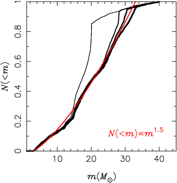
Figure 4: Cumulative distribution of the initial BH masses obtained from the stellar evolution calculations for $Z=(0.1,0.05,0.025,0.01)Z_{\odot}$, where line thickness decreases with increasing metallicity. The red line shows the cumulative distribution corresponding to the BH mass function $\phi\propto m^{\alpha}$ with $\alpha=0.5$ between $m_{\rm lo}=3\,{\rm M}_{\odot}$ and $m_{\rm up}=33\,{\rm M}_{\odot}$ which is a good approximation to the numerical results for $Z\lesssim 0.05Z_{\odot}$.

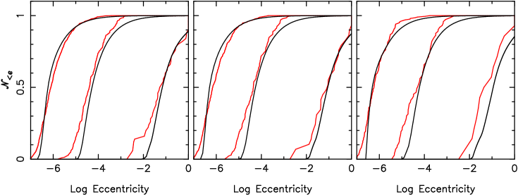
Figure 5: Comparison between the eccentricity distribution of the BH mergers produced in the Monte Carlo simulations of Rodriguez et al. (2018a) and those obtained with our method. Top panels show the cumulative distribution of $e$ for all mergers. In the bottom panels, the distributions of GW captures, in-cluster mergers, and mergers among ejected binaries are shown separately (from right to left, respectively). The distributions refer to binaries that merge after a given time from the start of the evolution, as indicated.

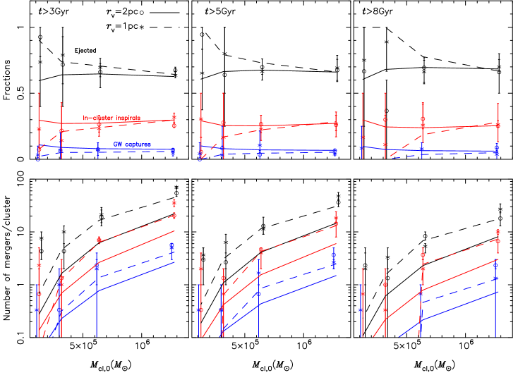
Figure 6: Fractions and total number of mergers for each of the three merger channels separately, at different times as a function of initial cluster mass obtained using our method (lines), and from the full Monte Carlo models of Rodriguez et al. (2018a) (symbols). Each point represents the average number of mergers from the three metallicities adopted in the Monte Carlo models.

3.4 Black hole masses

For the calculation of the merger rate and eccentricity distributions in BHBdynamics we need a model for the time evolution of the BH mass function. We assume that the BHs participating to the interactions have the same mass, i.e., $m_{1}=m_{2}=m_{3}$ and use $m_{\rm max}$ below to indicate the mass of each of the three BHs. The value of $m_{\rm max}$ is by definition restricted to the range of $\phi_{0}$, i.e. $m_{\rm lo}\leq m_{\rm max}\leq m_{\rm up}$. This choice is motivated by theory and detailed numerical models of dense star clusters (e.g., Sigurdsson & Hernquist, 1993; Rodriguez et al., 2016). Because of equipartition of energy, during a binary-single encounter the two heaviest objects in the interaction are the most likely to be paired together. Thus, after a few interactions the two BH components of a hard binary will have a similar mass. Moreover, because of mass segregation, the core densities will be dominated by the heaviest objects, so the BHs that the binary will encounter more frequently will have a mass comparable to the mass of its components, which are the most massive BHs still present in the cluster.

The cluster will process its BH population such that the mass of the ejected BHs progressively decreases with time as the most massive BHs are the first to form binaries and to be ejected from the cluster. Thus, in order to relate the evolution of $m_{\rm max}$ to the evolution of $M_{\rm BH}$ we compute the cumulative BH mass distribution (corrected by ejections due to SN kicks) and invert the relation to obtain an expression for the BH mass as a function of the current total mass in BHs. Hence, for a generic mass function $\phi$ (after SN kicks, see equation 2) we first solve $m_{\rm max}$ from

$$\int_{m_{\rm lo}}^{m_{\rm max}}\phi m{\rm d}m=M_{\rm BH},$$ (50)

where $M_{\rm BH}$ is provided by the cluster evolution (i.e. clusterBH). In some special cases, the solution for $m_{\rm max}$ can be written analytically, for example for a power-law $\phi_{0}\propto m^{\alpha}$ and no kicks (i.e. $\phi=\phi_{0}$) we find

$$m_{\rm max}=\left[{M_{\rm BH}\over M_{\rm BH,0}}\left(m_{\rm up}^{\alpha+2}-m_{\rm lo}^{\alpha+2}\right)+m_{\rm lo}^{\alpha+2}\right]^{1/(\alpha+2)},$$ (51)

where $M_{\rm BH,0}$ is the initial total mass in BHs. Initially, when $M_{\rm BH}=M_{\rm BH,0}$ we have $m_{\rm max}=m_{\rm up}$, while $m_{\rm max}=m_{\rm lo}$ for the last binary ejected from the cluster. Other prescriptions for $\phi_{0}$ and $\phi$ could also be implemented within our theoretical framework to describe higher metallicity systems and/or different natal kick prescriptions.

We assume that the BHs receive a natal kick given by the momentum conserving model described in Section 2.2. We then assume a power-law form for $\phi_{0}$, i.e. $\phi_{0}=Am^{\alpha}$, and for the purpose of finding $m_{\rm max}$ we approximate the mass function after kicks by equation (3). From integrating this function as in equation (50) we have

$$M_{\rm BH}(m_{\rm max})\simeq A\times\begin{cases}\displaystyle\ln{\left[\left(q_{\rm mb}^{3}+1\right)/\left(q_{\rm lb}^{3}+1\right)\right]},&\alpha=-2,\vspace{0.2cm}\\ \displaystyle m_{\rm max}^{\alpha+2}\left(1-h(q_{\rm mb})\right)-m_{\rm lo}^{\alpha+2}\left(1-h(q_{\rm lb})\right),&\alpha\neq-2,\end{cases}$$ (52)

where $q_{\rm ml}=m_{\rm max}/m_{\rm lo}$, and $q_{\rm mb}=m_{\rm max}/m_{\rm b}$. The constant $A$ is found from solving in a similar way $M_{\rm BH,0}f_{\rm ret}^{M}=\int_{m_{\rm lo}}^{m_{\rm up}}\phi m{\rm d}m$, which gives the same result as in equation (52), but with $m_{\rm max}$ replaced by $m_{\rm up}$ (see equation 5). The relation $M_{\rm BH}(m_{\rm max})$ of equation (52) needs to be computed once and can then be inverted numerically to get $m_{\rm max}$ for a given $M_{\rm BH}$.

Equations (51) and (52) apply only to systems for which $\phi_{0}$ can be described by a single power-law function. We now show that this is a good approximation for clusters with metallicity $Z\lesssim 0.05Z_{\odot}$. We obtained an approximation to the initial BH mass function using the Single Stellar Evolution (SSE) package (Hurley et al., 2002b) but with the updated prescriptions for stellar winds and mass loss in order to replicate the BH mass distribution of Dominik et al. (2013) and Belczynski et al. (2010). We sample the masses of the stellar progenitors from a mass function $\phi_{\star}\propto m_{\star}^{-2.35}$ (Kroupa et al., 2001). with masses in the range $20$ to $100\,{\rm M}_{\odot}$, and evolve the stars to BHs for the given metallicity. Fig. 4 shows that for metallicities $Z\lesssim 0.05Z_{\odot}$ the BH mass distribution can be fit by a power-low $\phi\propto m^{\alpha}$ with $\alpha=0.5$ between $m_{\rm lo}=3\,{\rm M}_{\odot}$ and $m_{\rm up}=33\,{\rm M}_{\odot}$. Because the metallicity distribution of GCs in the Milky Way peaks at about $Z\simeq 0.05Z_{\odot}$ (Zinn, 1985), this model can be used to provide a reasonably good approximation to the mass function of BHs formed in these systems. In what follows we will therefore adopt this model and use equation (51) or numerically determined inverse of equation (52) to describe the evolution of the BH mass function due to SN and/or dynamical kicks.

4 Comparison to Monte Carlo simulations

In this section we show that clusterBHBdynamics reproduces the eccentricty distribution, and rates of binary BH mergers formed in detailed Monte Carlo simulations of GCs as well as the evolution of the cluster itself. Specifically, we compare our results to the 24 GC Monte Carlo models of Rodriguez et al. (2016), Rodriguez et al. (2018a) and Rodriguez et al. (2018b). The model initial conditions are given in Table 1 in Rodriguez et al. (2016); these are 24 GC models with initial masses in the range $\simeq 10^{5}-10^{6}\,{\rm M}_{\odot}$, and virial radius $r_{\rm v}=1\,\rm pc$ or $\rm 2\,pc$ (where $r_{\rm h}\simeq 0.8r_{\rm v}$). For each value of mass and radius three different realisations with metallicity $Z=(0.01,\ 0.05,\ 0.25)Z_{\odot}$ were evolved for $\simeq 13\,\rm Gyr$ and during this time produced 2819 merging BH binaries, of which 1561 ($0.55$ of the total) were formed inside the cluster, and 123 ($0.04$ of the total) were GW captures. The rest of the mergers occurred among the population of ejected binaries. The Monte Carlo models are self-consistent simulations of the secular evolution of a cluster and include the effect of stellar evolution, a realistic mass function of stars, primordial binaries, the effect of an external tidal field and employ a three-body integrator (including post-Newtonian terms up to order 2.5) in order to accurately follow the strong binary-single interactions which lead to the hardening and merger of the core binaries.

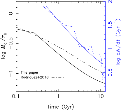
Figure 7: Evolution of the cluster compactness, that we define as $M_{\rm cl}/r_{\rm h}$, and the BH binary merger rate predicted by our method. We compare this to a similar Monte Carlo model from Rodriguez et al. (2018a). The cluster mass and radius have been normalised to their initial values $M_{\rm cl,0}=1.3\times 10^{6}\,{\rm M}_{\odot}$ and $r_{\rm h,0}=0.8\rm pc$.

For each value of cluster half-mass radius and total mass, we used equations (39) and (3.3) to compute the rate and eccentricity distribution of binary BH mergers that occur after a given time. Specifically we consider mergers that occur after $3$, $5$ and $8$ Gyr from the start of the simulation; if we assume that the clusters form at $z_{0}=3$, then, for the cosmological parameters above, these times correspond to binaries that merge within a redshift $z_{\rm d}\simeq 2,\ 1$ and $0.5$ respectively. The distributions from all the cluster models were then added together and compared to those from all the binary BH mergers produced in the Monte Carlo simulations. We only show the comparison for models where the BHs received the same momentum kick as neutron stars (with $\sigma_{\rm NS}=265~{}{\rm km\,s}^{-1}$). We note, however, that because of the high retention fractions in these systems, models without kicks applied to the BHs produce similar eccentricity distributions as models with kicks applied. Moreover, we use here an initial BH mass fraction $f_{\rm BH}=0.04$, appropriate for the low metallicity clusters considered.

Fig. 5 shows the eccentricity distributions at the moment the binaries first achieve a GW frequency of $10\,\rm Hz$ (i.e., near the low end of the LIGO-Virgo frequency window). The two methods give a very similar number of mergers at any given $e$ over the entire range of eccentricities (i.e., $e>10^{-7}$), and, for example, both produce $\sim 5\%$ of BH mergers with $e>0.1$ inside the LIGO-Virgo band. The individual eccentricity distributions of in-cluster mergers and mergers among the ejected binaries shown in the bottom panels also overlap reasonably well with those from the Monte Carlo simulations as do the fraction of mergers produced by each of the three channels (upper panels of Fig. 6), and the corresponding total number of mergers per cluster at a given time (lower panels of Fig. 6) for the entire cluster mass range considered.

In view of the approximate nature of our method, the agreement with the Monte Carlo results can appear quite remarkable. However, it is not a coincidence, but a rather natural consequence of Hénon’s principle. This principle, which is the basis of our approach, is also what determines the relation between the evolution of a cluster Monte Carlo model and the merger rate and properties of the BH binaries that are produced in its core. To illustrate this latter point, we plot in Fig. 7 the evolution of the global cluster ‘compactness’, defined here as $M_{\rm cl}/r_{\rm h}$, and the corresponding merger rate of BHs for a system with initial mass and radius $M_{\rm cl,0}=1.3\times 10^{6}\,{\rm M}_{\odot}$, $r_{\rm h,0}=0.8\,\rm pc$. We compare our results to those from a Monte Carlo cluster model with similar initial mass and radius (from Fig. 4 of Rodriguez et al., 2016). In both cases, two-body relaxation causes the cluster radius to expand significantly over the timescale of the simulation, leading to a decrease in the BH binary merger rate. The physical reason why the merger rate goes down is because the cluster energy demand decreases as the cluster expands and a significant drop in the binary hardening rate happens after about a relaxation time.

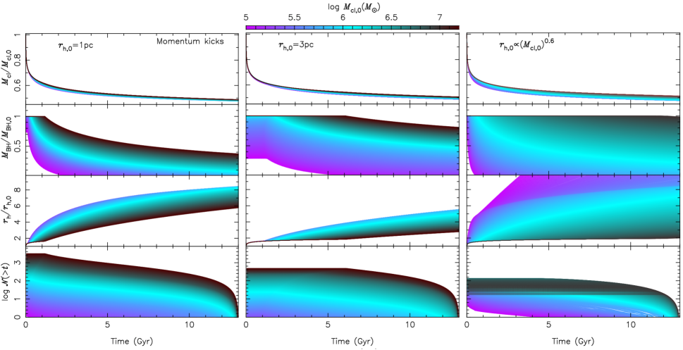
Figure 8: Evolution of cluster models for a range of masses and initial cluster radii. From top to bottom the panels show the evolution of the total mass of the clusters, the evolution of the mass in BHs, the cluster radius, and the number of BH binaries that merge after a given time from the start of the simulation. In this case we have adopted the momentum conserving natal kick model described in Section 2.2.

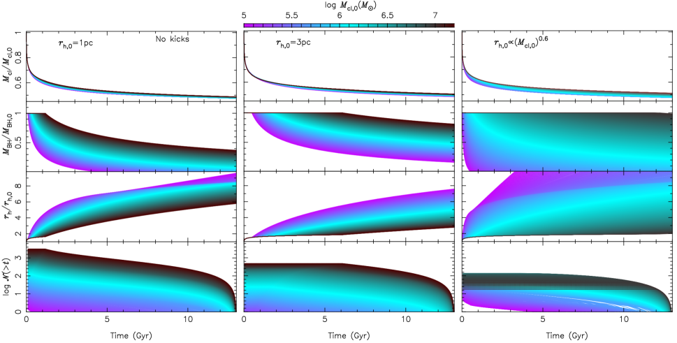
Figure 9: Same as Fig. 8 but for models where the BHs receive no natal kicks.

5 Astrophysical implications

In this section we use clusterBHBdynamics to derive the number and eccentricity distributions of merging BH binaries and study their relation to the initial properties of the parent cluster. Whilst a more detailed analysis will be presented elsewhere, here we simply consider how such distributions are linked to the initial mass and radius of a GC and its time evolution. The new method allows us to explore for the first time a wide range and physically motivated set of initial conditions, spanning more than two orders of magnitude both in radius and mass.

5.1 Cluster evolution and merger rates

We consider the evolution of a set of models with initial mass in the range $M_{\rm cl,0}\simeq(10^{5},\ 10^{7})\,{\rm M}_{\odot}$ that we evolved for 13 Gyrs. We adopt three different models for the initial radius of the clusters. We either assume that the initial radius is independent of mass and set $r_{\rm h,0}=1\,\rm pc$ or $3\,\rm pc$, or we assume an initial mass-radius relation (Gieles et al., 2010):

$$\log\left(r_{\rm h,0}\over{\rm pc}\right)=-3.560+0.615\log\left(M_{\rm cl,0}\over\,{\rm M}_{\odot}\right)\ .$$ (53)

This latter relation was obtained by converting the original Faber-Jackson relation of elliptical galaxies to a mass-radius relation (Hasegan et al., 2005), and correcting for the adiabatic expansion due to mass-loss caused by stellar evolution (Gieles et al., 2010). We show the results for models with constant momentum natal kicks and no natal kicks in Fig. 8 and Fig. 9, respectively. We take hereafter an initial BH mass fraction of $f_{\rm BH}=0.04$.

The top panels in Fig. 8 and Fig. 9 show that the total cluster mass has decreased by approximately a factor of two by the end of the simulation and that most of this mass-loss occurs during the first few Gyrs of evolution. Equation (7) implies that the fractional stellar mass-loss per unit time is the same for all clusters, so the small differences seen in the evolution of $M_{\rm cl}$ are a consequence of the dependence of $\dot{M}_{\rm BH}$ on the cluster relaxation time, and therefore on its mass and radius. The mass-loss from the system due to stellar evolution also causes the cluster radius to expand by approximately a factor 2. This can be seen in the figures at early times before the subsequent expansion due to two-body relaxation starts to dominate.

The top-middle panels in Fig.8 and Fig. 9 show that the evolution of the BH population is quite sensitive to the initial cluster properties. Systems that are initially more compact and with a low mass have a shorter relaxation time, and consequently they start to process their BH binaries at earlier times (i.e., at $t_{\rm cc}$) and at a higher rate than larger and more massive clusters (see equation 14). For example, the $r_{\rm h,0}\propto M_{\rm cl,0}^{0.6}$ models are highly dynamically active for $M_{\rm cl,0}\lesssim 10^{5}M_{\odot}$, yielding rate of cluster expansion, BH depletion, and number of merging binaries of larger magnitude than their $r_{\rm h,0}=1~{}$pc and 3 pc counterparts .

As a result of their long half-mass relaxation time, all cluster models with $M_{\rm cl,0}\gtrsim 10^{6}\,{\rm M}_{\odot}$ still have BHs after 13 Gyrs of evolution for the initial radii we adopted, corroborating the recent inference of stellar-mass BHs in $\omega$Cen (Zocchi et al., 2019; 2019MNRAS.488.5340B) and 47 Tuc (2019arXiv190808538H). Clusters with mass lower than this can also retain some of their black holes if their densities are sufficiently low initially (e.g., $r_{\rm h,0}=3\,\rm pc$). These results are also illustrated in Fig. 10 which gives the total mass in BHs at $t=13\,$Gyr for all the models considered. This figure demonstrates that the final number of BHs in clusters with $M_{\rm cl,0}\gtrsim 5\times 10^{5}\,{\rm M}_{\odot}$ does not depend significantly on the assumptions we make about the BH natal kicks. But, models with an initial mass lower than this value retain a significant fraction of their BHs only if no kicks are applied and the cluster initial radius is large, $r_{\rm h,0}=3\,\rm pc$. We conclude that whether a cluster will be able to retain some of its BHs depends on two main factors: the half-mass relaxation time of the whole system, which determines the rate at which the BHs are ejected from the cluster, and the initial BH fraction which is set by the stellar initial mass function, metallicity, and most importantly, by the natal kicks. These results are consistent with recent work based on Monte Carlo simulations (Askar et al., 2018; Kremer et al., 2019b), while extending these conclusions to a much wider region of relevant parameter space for star clusters.

After $t_{\rm cc}$, a system reaches balanced evolution, and its half-mass radius starts to increase as the result of two-body relaxation. The evolution of $r_{\rm h}$ for our models appears to be very sensitive to the initial conditions. Generally, systems that have a shorter half-mass relaxation time expand faster and end up with a larger $r_{\rm h}$ after a Hubble time. The evolution of the cluster radius should also depend on metallicity, the initial stellar mass function, and the assumed natal kick distribution because these set the initial fraction of BHs, which changes $t_{\rm rh}$ through the parameter $\psi$. The effect of natal kicks becomes especially important in systems with a low mass ($M_{\rm cl,0}\lesssim 5\times 10^{5}\,{\rm M}_{\odot}$) and a large half-mass radius ($r_{\rm h,0}\gtrsim 3\,\rm pc$) due to the larger fraction of BHs that are ejected. These results fit in the view that the properties of the whole system determine the evolution of the BH sub-system (Breen & Heggie, 2013), but the evolution of the cluster itself is also affected by the remaining mass fraction in BHs (Section 2.3).

The total number of BH binaries that merge at times $>t$ can be seen in the bottom panels of Fig. 8 and Fig. 9. Clusters with a longer relaxation time start forming binary BHs later, which explains the initial lag between the start of the simulation and when the first merger occurs (i.e., the plateau of $\mathcal{N}(>t)$ seen at early times). The BH binary merger rate is shown as a function of cluster properties in Fig. 11. Assuming a constant initial radius, the total number of BH binaries that merge at late times ($t>8\,$Gyr) can be reasonably well fit by a simple scaling $\mathcal{N}\propto M_{\rm cl,0}^{1.6}$. For the relation equation (53), instead, the best fit model is $\mathcal{N}\propto M_{\rm cl,0}^{1.2}$, for $M_{\rm cl,0}\lesssim 10^{7}\,{\rm M}_{\odot}$, while for more massive clusters the segregation timescale of the BHs exceeds the Hubble time and no mergers are produced in these systems. Taken together, our results imply that $\mathcal{N}\propto M_{\rm cl,0}^{1.6}r_{\rm h,0}^{-2/3}$. These results can be compared to Hong et al. (2018) who find that the total number of mergers produced by their cluster models over 12 Gyr scaled as $\mathcal{N}\propto M_{\rm cl,0}^{1.3}r_{\rm h,0}^{-0.9}$. The difference with our best fit model could be due to the larger parameter space explored by us and by the fact that these authors did not include in-cluster mergers in their Monte Carlo simulations.

Figure 10: Mass in BHs left after 13 Gyrs of evolution as a function of initial cluster mass for the systems of Fig. 8 and Fig. 9.

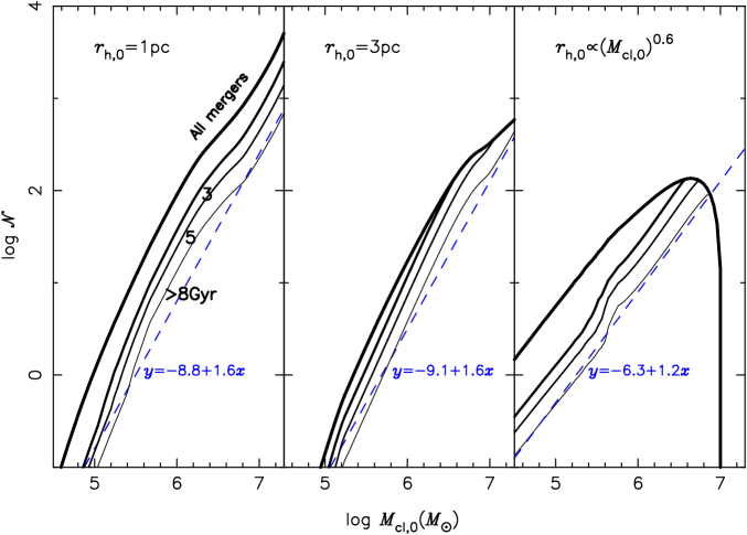
Figure 11: Number of merging binaries as a function of cluster mass for the models of Fig. 8 where the BHs receive the same momentum kick as neutron stars. From top to bottom line, we show the number of binaries which merge at times $t>0$, 3, 5, and 8 Gyr from the start of the simulation. Blue lines show the best fit models to the mergers that occur at late times.

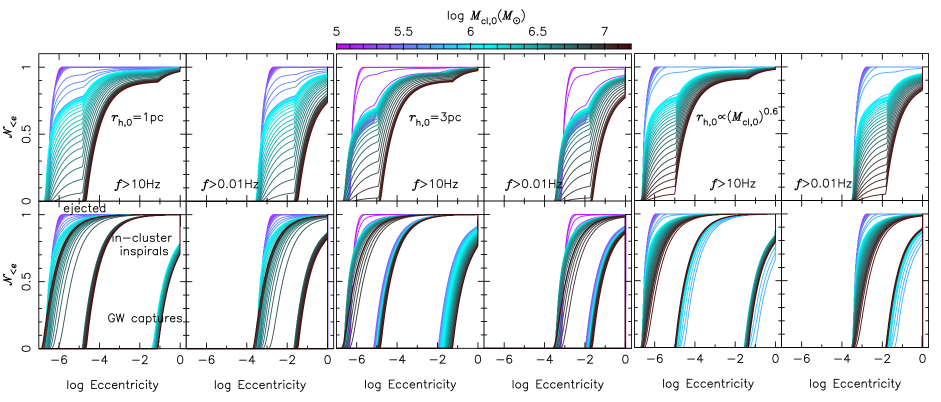
Figure 12: Eccentricity distributions of merging BH binaries formed in star clusters for the three choices of $r_{\rm h,0}$, at the moment their GW frequency becomes larger than $10$ and $0.01$ Hz. Bottom panels give the eccentricity distributions for ejected binaries (lowest eccentricities), in-cluster inspirals and GW captures (largest eccentricities) separately. Note that at $0.01$ Hz, GW captures all have $e\simeq 1$ because thy all form at frequencies $f>0.1\,$Hz. In this calculation we have adopted the constant momentum natal kick model of Section 2.2, and we have only included late time mergers, occurring at $t>8$ Gyr.

As a general trend, we observe a strong dependence of the merger rate on the cluster initial conditions, with a larger cluster mass and a smaller radius resulting into an overall higher BH merger rate. These results put into question some of the current literature where simplified assumptions about the initial mass/half-mass radius relation were adopted. For example, Rodriguez & Loeb (2018) derived their binary BH merger rate assuming that $50\%$ of clusters form with a virial radius of $r_{\rm v}=1\,$pc and $50\%$ form with $r_{\rm v}=2\,$pc. Similarly, Fragione & Kocsis (2018) assumed that the binary BH merger rate is independent of the cluster radius for which they assumed a fixed value. Askar et al. (2017) derived a merger rate by using a limited set of models with three values of cluster initial radii and four values of cluster mass. These restrictions were due to time constraints imposed by the computationally expensive techniques employed in these studies. Although our models include less physics, the new treatment allows for a complete exploration of the parameter space relevant for GCs. This opens the possibility for a first realistic determination of the merger rate and properties of BH binaries produced in star clusters which we reserve to a future paper. We note that a similar attempt was made before in Choksi et al. (2019) who adopted the semi-analytical approach of Antonini & Rasio (2016) to estimate a cosmic black hole merger rate from GCs. In Antonini & Rasio (2016), however, the binary hardening rate was computed from the cluster core density which cannot be easily linked to the secular evolution of a cluster. Here, we have overcome this issue by using Hénon’s principle to relate the binary hardening rate to the evolving global properties of its host cluster.

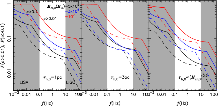
Figure 13: Fraction of binaries that have an eccentricity larger than $0.1$ and $0.01$ as a function of peak GW frequency. We have considered three representative values of cluster mass for our three choices of radius, have adopted the natal kick model of Section 2.2, and only binaries that merge after a time larger than 8 Gyr from the start of the simulation have been included in the analysis.

Figure 14: Number of BH binaries that merge after $8$ Gyr as a function of cluster mass, for the models of Fig. 8 and for the three merger channels shown separately.

5.2 Eccentricity distributions

Binary black holes formed in dynamical environments, such as globular clusters, and nuclear star clusters, can have a finite eccentricity in both LIGO-Virgo, and the LISA bands (e.g., Nishizawa et al., 2016). For mergers formed through the evolution of field binaries instead, any eccentricity is washed out by GW radiation by the time the signal enters the detector frequency band (Belczynski et al., 2002). As a non-zero eccentricity would be a unique fingerprint of a dynamical origin, we focus in this section on the relation between a cluster properties and the eccentricity distribution of the BH binary mergers that it produces.

In Fig. 12 we show the eccentricity distribution of the merging BH binaries. We focus here on mergers occurring at late times ($t>$8 Gyr) because these are the most relevant for current and planned GW detectors. If we assume that the clusters form at $z_{0}=3$, then, for the cosmological parameters above, this time corresponds to binaries that merge within a redshift $z_{\rm d}=0.5$. We show these distributions for several values of $M_{\rm cl}$, for our three choices of cluster radius, and at the moment the binary GW frequency first becomes larger than $10$ and $0.01$ Hz. We chose to plot the eccentricity distributions at $10$ and $0.01$ Hz because these are near the lower end of the LIGO-Virgo and LISA frequency windows respectively (Harry & LIGO Scientific Collaboration, 2010; Amaro-Seoane et al., 2017). In the bottom panels the cumulative eccentricity distributions of in-cluster inspirals, GW captures, and mergers among the ejected binaries are shown separately.

Our analysis demonstrates that independently of the cluster initial conditions, GW captures have $e>10^{-2}$ at $f>10\,\rm Hz$, while all other type of mergers have eccentricities at these frequencies ($e\lesssim 10^{-2}$) that might be too small to be measurable using current detectors (e.g., Huerta & Brown, 2013; Lower et al., 2018; Gondán & Kocsis, 2019). As expected, mergers among the ejected binaries have the smallest eccentricities. We conclude that GW captures are the only type of mergers that we have considered in our analysis which could have a measurable residual eccentricity at the moment they enter the LIGO-Virgo frequency window. At $f>10\,\rm Hz$, in-cluster mergers show a clear tri-modality, with the lower peak corresponding to isolated binaries that merge after a dynamical encounter, the higher eccentricity population ($0.1<e<1$) corresponding to sources which merge during an encounter via a GW capture, and a third population of mergers with $e\simeq 1$. These latter systems also merge through a GW capture, but form directly at frequencies larger than $10\rm Hz$ rather than reaching this frequency after substantial circularisation has already occurred.

Because all GW captures are formed at frequencies above $\simeq 0.1\rm Hz$, the eccentricity distributions of these mergers appears as a delta function at $e=1$ for the lowest frequency range considered in Fig. 12. As shown in Chen & Amaro-Seoane (2017), these highly eccentric sources might elude detection because the high eccentricity shifts the peak of the relative power of the GW harmonics towards higher frequencies, so that their maximum power is emitted farther away from the frequency band of interest. Mergers formed by GW captures are therefore unlikely to be detectable at frequencies lower than $0.1\rm Hz$. On the other hand, for $M_{\rm cl,0}\gtrsim 10^{6}\,{\rm M}_{\odot}$ we see that all in-cluster inspirals reach $f=0.01\rm Hz$ with $e\gtrsim 0.01$, which is potentially measurable with planned missions such as LISA (Nishizawa et al., 2016) and third generation detectors (Punturo et al., 2010).

The fraction of eccentric GW sources is shown in Fig. 13 as a function of the peak frequency $f$ and for three representative values of cluster mass. From this plot we see that between $\approx 30$ to $100\%$ of our binaries start eccentric inside the LISA frequency window ($0.001-0.1\rm Hz$), and many retain a significant eccentricity by the time they reach $f\simeq 0.01\rm Hz$ where LISA is most sensitive. The exact fraction of systems that start eccentric in the LISA band depends on the cluster properties, reaching unity for $M_{\rm cl,0}\simeq 10^{7}\,{\rm M}_{\odot}$. This is different from BH binary mergers formed from the evolution of field binaries of which only $\lesssim 10\%$ are expected to have $e>0.01$ at $f=0.001\rm Hz$ (Breivik et al., 2016). We conclude that sufficient observations of the eccentricity of binaries in the LISA band could be used to discriminate between formation in the field and in clusters (e.g., Nishizawa et al., 2016), but could also help to determine which type of clusters are most likely to produce the binaries.

The overall eccentricity distribution of the BH binaries is most sensitive to the relative fraction of the three type of mergers. We show how these fractions depend on the cluster properties in Fig. 14. Three regimes can be identified: (i) if $a_{\rm GW}>a_{\rm ej}$ all binary black hole mergers are produced inside the cluster. About $\lesssim 10\%$ of these in-cluster mergers are GW captures and the rest are mergers that occur in between binary-single encounters. For the systems in Fig. 14 this regime can be seen at $M_{\rm cl,0}\gtrsim 10^{7}\,{\rm M}_{\odot}$; (ii) when $a_{\rm GW}<a_{\rm ej}$ almost half of the mergers occur inside the cluster, half are mergers among the ejected binaries, and less than a few per cent of the mergers are GW captures. For the clusters in Fig. 14 this regime occurs at $10^{6}\,{\rm M}_{\odot}\lesssim M_{\rm cl,0}\lesssim 10^{7}\,{\rm M}_{\odot}$; (ii) if the BH binary population has been fully depleted by a time $t$, then all mergers observed at later times will come from the ejected binary population. This third regime occurs for the lowest mass systems in Fig. 14 where we see that the number of in-cluster mergers goes to zero. The exact transition between the three regimes depends on the initial mass-radius relation and the time between the formation of the cluster and when the mergers are detected.

Our results show that for a typical GC the fraction of in-cluster mergers can be quite large, in agreement with recent studies showing that nearly half of all binary black hole mergers occur inside the cluster (Samsing, 2018; Rodriguez et al., 2018a). On the other hand, our models also show that the number of in-cluster mergers detectable by LIGO-Virgo will be quite sensitive to the uncertain initial cluster mass-radius relation and initial mass distribution of the clusters. Notably, in the most massive GCs ($M_{\rm cl,0}\gtrsim 10^{6}\,{\rm M}_{\odot}$) we would expect a large fraction ($\gtrsim 0.5$) of mergers to be produced inside the cluster rather than happening among the ejected binaries. In even higher velocity dispersion clusters such as nuclear clusters, all mergers should typically be formed while the BH binaries are still bound to the cluster, although a significant contribution from the ejected population might be expected near the low end of the nuclear cluster mass distribution (Antonini & Rasio, 2016).

We note, finally, that detailed post-Newtonian direct $N$-body simulations show that in low mass clusters ($M_{\rm cl}\lesssim 10^{5}M_{\odot}$), in-cluster mergers are primarily triggered by long-term interactions involving stable and marginally stable triples (Ziosi et al., 2014; Kimpson et al., 2016a; Banerjee, 2017, 2018a, 2018b; Rastello et al., 2019). A large fraction of these mergers will have a finite eccentricity in the LIGO band but are not included in our analysis.

5.3 Caveats and discussion

In deriving the merger probability and eccentricity distributions above we have made a few important assumptions which we now discuss and justify.

We have assumed that the dynamical interactions only occur between BHs. This is reasonable because due to mass segregation the BH densities near the core are expected to be much larger than the densities of stars. BHs will therefore dominate the interactions. Moreover, because exchange interactions tend to pair the BHs with the highest mass and tens of three body encounters are required before a merger, then mergers will be primarily between BHs when they are present (e.g., Sigurdsson & Hernquist, 1993; Morscher et al., 2015b). As the number of BHs in the core decreases, interactions with main sequence stars, giant, and white dwarfs can become more frequent. These interactions could lead to the formation of mass-transferring binaries with an observable electromagnetic signature (e.g., Fabian et al., 1975; Ivanova et al., 2010), or detached BH-stellar binaries that can be identified with radial velocities (2018MNRAS.475L..15G). Note also that the removal of BHs strictly from the upper end of its mass distribution and the interactions among the most massive BH members, as assumed here, is an idealisation. Detailed $N$-body computations suggest that dynamically assembled binaries span over a mass ratio between $0.5-1$ (Banerjee, 2017, 2018b), implying that BHs over a considerable mass range could be involved in mutual encounters.

The eccentricity distributions were derived by assuming that the binaries have a large eccentricity, $e_{0}\approx 1$ , at the moment their evolution starts to be dominated by GW radiation. This allowed us to find the simple analytical relation equation (44) between the eccentricity of a binary and its peak GW frequency. The assumption of high initial eccentricity is reasonable for in-cluster mergers, but might not be valid for some fraction of the mergers occurring among the ejected binaries (Kremer et al., 2019a). The eccentricity distribution of all ejected binaries is thermal, but for the subset of these binaries that merge within one Hubble time the distribution is skewed towards higher eccentricities. Thus, we expect our approximation to hold as long as $p_{\rm ex}(a_{\rm ej})\ll 1$, and to progressively worsen as $p_{\rm ex}(a_{\rm ej})$ increases. By setting $p_{\rm ex}(a_{\rm ej})=1$ and solving for $v_{\rm esc}$ we find that for escape velocities larger than

$${v}_{\rm ex}\simeq 19\,{\rm km\ s^{-1}}\left({m_{1}m_{2}\over m_{123}}q_{3}{6\over{{\rm M}_{\odot}}}\right)^{1/2}\left({{\rm 10\,Gyr}\over\tau}\right)^{1/8}\ ,$$ (54)

all ejected binaries will merge and their eccentricity distribution will be thermal. Even in this case, however, the overall impact on the eccentricity distribution should not be great as only about $10\%$ of the ejected binaries have $e_{0}<0.3$. Moreover, the contribution of the ejected binaries becomes less important for the more massive clusters that satisfy the condition $v_{\rm esc}>\tilde{v}_{\rm ex}$ (see Section 5.2).

We note also that our calculation is based on the assumption that most binary BH mergers are formed through strong binary-single interactions. However, BH mergers in star clusters can also occur through other processes which have not be considered in our analysis. These include mergers mediated by the Lidov-Kozai mechanism in hierarchical triples (Miller & Hamilton, 2002; Wen, 2003; Kimpson et al., 2016b), non-hierarchical triples (Antonini et al., 2014, 2016; Arca-Sedda et al., 2018), mergers from direct BH-BH captures (Quinlan & Shapiro, 1990; Kocsis & Levin, 2012; Rasskazov & Kocsis, 2019), and eccentric mergers during binary-binary strong interactions (Zevin et al., 2019). All these effects are believed to play only a marginal role (at a $\sim 1\%$ level) for the BH merger rate, but might somewhat increase the number of binaries that enter the LIGO-Virgo frequency band with a large eccentricity. More recently, Hamers & Samsing (2019) and Samsing et al. (2019b) argued that weak fly-by encounters could also affect the eccentricity distributions of in-cluster mergers.

Finally, primordial binaries which are not considered here are an essential ingredient of the early dynamical evolution of globular clusters and their young progenitors. The presence of primordial binaries would make the BH core-driven balanced evolution (and hence $t_{\rm cc}$) less defined since they would be an ambient source of central energy generation from the beginning of the cluster’s evolution. After the segregation of BHs, the central energy generation will be shared with the primordial binaries which could potentially affect the relevant encounter rates among the BHs.

References

- Aarseth (1999) Aarseth S. J., 1999, PASP, 111, 1333
- Aarseth (2003) Aarseth S. J., 2003, Gravitational N-Body Simulations. Cambridge University Press, November 2003.
- Aarseth (2012) Aarseth S. J., 2012, Monthly Notices of the Royal Astronomical Society, 422, 841
- Abadie et al. (2010) Abadie J., et al., 2010, Classical and Quantum Gravity, 27, 173001
- Abbott et al. (2016a) Abbott B. P., et al., 2016a, Physical Review X, 6, 041015
- Abbott et al. (2016b) Abbott B. P., et al., 2016b, Phys. Rev. Lett., 116, 061102
- Abbott et al. (2018) Abbott B. P., et al., 2018, Living Reviews in Relativity, 21, 3
- Acernese et al. (2015) Acernese F., et al., 2015, Classical and Quantum Gravity, 32, 024001
- Ahmad & Cohen (1973) Ahmad A., Cohen L., 1973, Journal of Computational Physics, 12, 389
- Alexander & Gieles (2012) Alexander P. E. R., Gieles M., 2012, MNRAS, 422, 3415
- Alexander et al. (2014) Alexander P. E. R., Gieles M., Lamers H. J. G. L. M., Baumgardt H., 2014, Monthly Notices of the Royal Astronomical Society, 442, 1265
- Amaro-Seoane et al. (2017) Amaro-Seoane P., et al., 2017, arXiv e-prints, p. arXiv:1702.00786
- Antonini & Rasio (2016) Antonini F., Rasio F. A., 2016, ApJ, 831, 187
- Antonini et al. (2014) Antonini F., Murray N., Mikkola S., 2014, ApJ, 781, 45
- Antonini et al. (2016) Antonini F., Chatterjee S., Rodriguez C. L., Morscher M., Pattabiraman B., Kalogera V., Rasio F. A., 2016, ApJ, 816, 65
- Antonini et al. (2017) Antonini F., Toonen S., Hamers A. S., 2017, ApJ, 841, 77
- Antonini et al. (2019) Antonini F., Gieles M., Gualandris A., 2019, MNRAS, 486, 5008
- Arca-Sedda et al. (2018) Arca-Sedda M., Li G., Kocsis B., 2018, arXiv e-prints, p. arXiv:1805.06458
- Askar et al. (2017) Askar A., Szkudlarek M., Gondek-Rosińska D., Giersz M., Bulik T., 2017, MNRAS, 464, L36
- Askar et al. (2018) Askar A., Arca Sedda M., Giersz M., 2018, MNRAS, 478, 1844
- Banerjee (2017) Banerjee S., 2017, MNRAS, 467, 524
- Banerjee (2018a) Banerjee S., 2018a, MNRAS, 473, 909
- Banerjee (2018b) Banerjee S., 2018b, MNRAS, 481, 5123
- Banerjee & Kroupa (2017) Banerjee S., Kroupa P., 2017, A&A, 597, A28
- Banerjee et al. (2019) Banerjee S., Belczynski K., Fryer C. L., Berczik P., Hurley J. R., Spurzem R., Wang L., 2019, arXiv:1902.07718,
- Baumgardt & Makino (2003) Baumgardt H., Makino J., 2003, Monthly Notices of the Royal Astronomical Society, 340, 227
- Belczynski et al. (2002) Belczynski K., Kalogera V., Bulik T., 2002, ApJ, 572, 407
- Belczynski et al. (2010) Belczynski K., Dominik M., Bulik T., O?Shaughnessy R., Fryer C., Holz D. E., 2010, The Astrophysical Journal, 715, L138
- Breen & Heggie (2011) Breen P. G., Heggie D. C., 2011, Monthly Notices of the Royal Astronomical Society, 420, 13
- Breen & Heggie (2013) Breen P. G., Heggie D. C., 2013, Monthly Notices of the Royal Astronomical Society, 432, 2779
- Breivik et al. (2016) Breivik K., Rodriguez C. L., Larson S. L., Kalogera V., Rasio F. A., 2016, ApJ, 830, L18
- Cao & Han (2017) Cao Z., Han W.-B., 2017, Phys. Rev. D, 96, 044028
- Chen & Amaro-Seoane (2017) Chen X., Amaro-Seoane P., 2017, ApJ, 842, L2
- Choksi et al. (2019) Choksi N., Volonteri M., Colpi M., Gnedin O. Y., Li H., 2019, ApJ, 873, 100
- Di Carlo et al. (2019) Di Carlo U. N., Giacobbo N., Mapelli M., Pasquato M., Spera M., Wang L., Haardt F., 2019, MNRAS, 487, 2947
- Dominik et al. (2012) Dominik M., Belczynski K., Fryer C., Holz D. E., Berti E., Bulik T., Mandel I., O’Shaughnessy R., 2012, DOUBLE COMPACT OBJECTS. I. THE SIGNIFICANCE OF THE COMMON ENVELOPE ON MERGER RATES, doi:10.1088/0004-637X/759/1/52, http://adslabs.org/adsabs/abs/2012ApJ...759...52D/
- Dominik et al. (2013) Dominik M., Belczynski K., Fryer C., Holz D. E., Berti E., Bulik T., Mandel I., O’Shaughnessy R., 2013, The Astrophysical Journal, 779, 72
- Downing et al. (2011) Downing J. M. B., Benacquista M. J., Giersz M., Spurzem R., 2011, Monthly Notices of the Royal Astronomical Society, pp no–no
- Fabian et al. (1975) Fabian A. C., Pringle J. E., Rees M. J., 1975, MNRAS, 172, 15p
- Foreman-Mackey et al. (2013) Foreman-Mackey D., Hogg D. W., Lang D., Goodman J., 2013, PASP, 125, 306
- Fragione & Kocsis (2018) Fragione G., Kocsis B., 2018, Phys. Rev. Lett., 121, 161103
- Fragione & Kocsis (2019) Fragione G., Kocsis B., 2019, MNRAS, 486, 4781
- Fryer & Kalogera (2001) Fryer C. L., Kalogera V., 2001, The Astrophysical Journal, 554, 548
- Gerosa et al. (2018) Gerosa D., Berti E., O’Shaughnessy R., Belczynski K., Kesden M., Wysocki D., Gladysz W., 2018, Phys. Rev. D, 98, 084036
- Gieles et al. (2010) Gieles M., Baumgardt H., Heggie D. C., Lamers H. J. G. L. M., 2010, MNRAS, 408, L16
- Gieles et al. (2011) Gieles M., Heggie D. C., Zhao H., 2011, MNRAS, 413, 2509
- Gieles et al. (2014) Gieles M., Alexander P. E. R., Lamers H. J. G. L. M., Baumgardt H., 2014, MNRAS, 437, 916
- Giersz (1998) Giersz M., 1998, Monthly Notices of the Royal Astronomical Society, 298, 1239
- Giersz & Heggie (1997) Giersz M., Heggie D. C., 1997, MNRAS, 286, 709
- Giersz et al. (2013) Giersz M., Heggie D. C., Hurley J. R., Hypki A., 2013, Monthly Notices of the Royal Astronomical Society, 431, 2184
- Gondán & Kocsis (2019) Gondán L., Kocsis B., 2019, ApJ, 871, 178
- Goodman (1984) Goodman J., 1984, ApJ, 280, 298
- Goodman & Weare (2010) Goodman J., Weare J., 2010, Communications in Applied Mathematics and Computational Science, Vol.~5, No.~1, p.~65-80, 2010, 5, 65
- Gültekin et al. (2006) Gültekin K., Miller M. C., Hamilton D. P., 2006, ApJ, 640, 156
- Hamers & Samsing (2019) Hamers A. S., Samsing J., 2019, arXiv e-prints, p. arXiv:1904.09624
- Harry & LIGO Scientific Collaboration (2010) Harry G. M., LIGO Scientific Collaboration 2010, Classical and Quantum Gravity, 27, 084006
- Ha\textcommabelowsegan et al. (2005) Ha\textcommabelowsegan M., et al., 2005, ApJ, 627, 203
- Heggie (1975) Heggie D. C., 1975, Monthly Notices of the Royal Astronomical Society, 173, 729
- Heggie & Aarseth (1992) Heggie D. C., Aarseth S. J., 1992, MNRAS, 257, 513
- Heggie & Hut (2003) Heggie D., Hut P., 2003, The Gravitational Million-Body Problem: A Multidisciplinary Approach to Star Cluster Dynamics, by Douglas Heggie and Piet Hut. Cambridge University Press, 2003, 372 pp.
- Hénon (1961) Hénon M., 1961, Annales d’Astrophysique, 24, 369
- Hénon (1975) Hénon M., 1975, in Hayli A., ed., IAU Symposium Vol. 69, Dynamics of the Solar Systems. p. 133
- Hinder et al. (2018) Hinder I., Kidder L. E., Pfeiffer H. P., 2018, Phys. Rev. D, 98, 044015
- Hobbs et al. (2005) Hobbs G., Lorimer D. R., Lyne A. G., Kramer M., 2005, Monthly Notices of the Royal Astronomical Society, 360, 974
- Hong et al. (2018) Hong J., Vesperini E., Askar A., Giersz M., Szkudlarek M., Bulik T., 2018, MNRAS, 480, 5645
- Huerta & Brown (2013) Huerta E. A., Brown D. A., 2013, Phys. Rev. D, 87, 127501
- Huerta et al. (2019) Huerta E. A., et al., 2019, arXiv e-prints, p. arXiv:1901.07038
- Hurley et al. (2000) Hurley J. R., Pols O. R., Tout C. A., 2000, MNRAS, 315, 543
- Hurley et al. (2002a) Hurley J. R., Tout C. A., Pols O. R., 2002a, MNRAS, 329, 897
- Hurley et al. (2002b) Hurley J. R., Tout C. A., Pols O. R., 2002b, MNRAS, 329, 897
- Ivanova et al. (2005) Ivanova N., Belczynski K., Fregeau J. M., Rasio F. A., 2005, Monthly Notices of the Royal Astronomical Society, 358, 572
- Ivanova et al. (2010) Ivanova N., Chaichenets S., Fregeau J., Heinke C. O., Lombardi Jr. J. C., Woods T. E., 2010, ApJ, 717, 948
- Joshi et al. (2000) Joshi K. J., Rasio F. A., Portegies Zwart S., 2000, ApJ, 540, 969
- Katz & Dong (2012) Katz B., Dong S., 2012, arXiv e-prints, p. arXiv:1211.4584
- Kim et al. (1998) Kim S. S., Lee H. M., Goodman J., 1998, ApJ, 495, 786
- Kimpson et al. (2016a) Kimpson T. O., Spera M., Mapelli M., Ziosi B. M., 2016a, MNRAS, 463, 2443
- Kimpson et al. (2016b) Kimpson T. O., Spera M., Mapelli M., Ziosi B. M., 2016b, Monthly Notices of the Royal Astronomical Society, 463, 2443
- Kocsis & Levin (2012) Kocsis B., Levin J., 2012, Physical Review D, 85, 123005
- Kremer et al. (2019a) Kremer K., et al., 2019a, Phys. Rev. D, 99, 063003
- Kremer et al. (2019b) Kremer K., Chatterjee S., Ye C. S., Rodriguez C. L., Rasio F. A., 2019b, ApJ, 871, 38
- Kroupa et al. (2001) Kroupa P., Aarseth S., Hurley J., 2001, MNRAS, 321, 699
- Kulkarni et al. (1993) Kulkarni S. R., Hut P., McMillan S. J., 1993, Nature, 364, 421
- Leigh et al. (2018) Leigh N. W. C., et al., 2018, MNRAS, 474, 5672
- Liu & Lai (2019) Liu B., Lai D., 2019, MNRAS, 483, 4060
- Lower et al. (2018) Lower M. E., Thrane E., Lasky P. D., Smith R., 2018, Phys. Rev. D, 98, 083028
- Makino & Aarseth (1992) Makino J., Aarseth S. J., 1992, PASJ, 44, 141
- Mandel (2016) Mandel I., 2016, MNRAS, 456, 578
- Mandel & De Mink (2016) Mandel I., De Mink S. E., 2016, MNRAS, 458, 2634
- Marchant et al. (2016) Marchant P., Langer N., Podsiadlowski P., Tauris T. M., Moriya T. J., 2016, A&A, 588
- Michaely & Perets (2019) Michaely E., Perets H. B., 2019, arXiv e-prints, p. arXiv:1902.01864
- Miller & Hamilton (2002) Miller M. C., Hamilton D. P., 2002, ApJ, 576, 894
- Miller & Lauburg (2009) Miller M. C., Lauburg V. M., 2009, ApJ, 692, 917
- Morscher et al. (2015a) Morscher M., Pattabiraman B., Rodriguez C., Rasio F. A., Umbreit S., 2015a, The Astrophysical Journal, 800, 9
- Morscher et al. (2015b) Morscher M., Pattabiraman B., Rodriguez C., Rasio F. A., Umbreit S., 2015b, ApJ, 800, 9
- Nishizawa et al. (2016) Nishizawa A., Berti E., Klein A., Sesana A., 2016, Phys. Rev. D, 94, 064020
- Nitadori & Aarseth (2012) Nitadori K., Aarseth S. J., 2012, MNRAS, 424, 545
- Peters (1964) Peters P., 1964, Physical Review, 136, B1224
- Peuten et al. (2017) Peuten M., Zocchi A., Gieles M., Hénault-Brunet V., 2017, MNRAS, 470, 2736
- Planck Collaboration et al. (2015) Planck Collaboration et al., 2015
- Plummer (1911) Plummer H. C., 1911, MNRAS, 71, 460
- Portegies Zwart & McMillan (2000) Portegies Zwart S. F., McMillan S. L. W., 2000, ApJ, 528, L17
- Portegies Zwart et al. (2010) Portegies Zwart S. F., McMillan S. L. W., Gieles M., 2010, Annual Review of Astronomy and Astrophysics, 48, 431
- Punturo et al. (2010) Punturo M., et al., 2010, Classical and Quantum Gravity, 27, 084007
- Quinlan & Shapiro (1990) Quinlan G. D., Shapiro S. L., 1990, ApJ, 356, 483
- Rasskazov & Kocsis (2019) Rasskazov A., Kocsis B., 2019, arXiv e-prints, p. arXiv:1902.03242
- Rastello et al. (2019) Rastello S., Amaro-Seoane P., Arca-Sedda M., Capuzzo-Dolcetta R., Fragione G., Tosta e Melo I., 2019, MNRAS, 483, 1233
- Rodriguez & Loeb (2018) Rodriguez C. L., Loeb A., 2018, ApJ, 866, L5
- Rodriguez et al. (2015) Rodriguez C. L., Morscher M., Pattabiraman B., Chatterjee S., Haster C.-J., Rasio F. A., 2015, Physical Review Letters, 115, 051101
- Rodriguez et al. (2016) Rodriguez C. L., Chatterjee S., Rasio F. A., 2016, Physical Review D, 93, 084029
- Rodriguez et al. (2018a) Rodriguez C. L., Amaro-Seoane P., Chatterjee S., Kremer K., Rasio F. A., Samsing J., Ye C. S., Zevin M., 2018a, Phys. Rev. D, 98, 123005
- Rodriguez et al. (2018b) Rodriguez C. L., Amaro-Seoane P., Chatterjee S., Rasio F. A., 2018b, Phys. Rev. Lett., 120, 151101
- Samsing (2018) Samsing J., 2018, Phys. Rev. D, 97, 103014
- Samsing et al. (2014) Samsing J., MacLeod M., Ramirez-Ruiz E., 2014, The Astrophysical Journal, 784, 71
- Samsing et al. (2019a) Samsing J., Venumadhav T., Dai L., Martinez I., Batta A., Lopez Martin J., Ramirez-Ruiz E., Kremer K., 2019a, arXiv e-prints, p. arXiv:1901.02889
- Samsing et al. (2019b) Samsing J., Hamers A. S., Tyles J. G., 2019b, arXiv e-prints, p. arXiv:1906.07189
- Sesana (2016) Sesana A., 2016, Phys. Rev. Lett., 116, 231102
- Sigurdsson & Hernquist (1993) Sigurdsson S., Hernquist L., 1993, Nature, 364, 423
- Silsbee & Tremaine (2017) Silsbee K., Tremaine S., 2017, The Astrophysical Journal, 836, 39
- Spera et al. (2015) Spera M., Mapelli M., Bressan A., 2015, Monthly Notices of the Royal Astronomical Society, 451, 4086
- Spitzer (1969) Spitzer L. J., 1969, The Astrophysical Journal, 158, L139
- Spitzer (1987) Spitzer L., 1987, Dynamical evolution of globular clusters. Princeton Univ. Press, Princeton, NJ
- Spitzer & Hart (1971) Spitzer Jr. L., Hart M. H., 1971, ApJ, 164, 399
- Wang et al. (2016) Wang L., et al., 2016, MNRAS, 458, 1450
- Wen (2003) Wen L., 2003, The Astrophysical Journal, 598, 419
- Zevin et al. (2019) Zevin M., Samsing J., Rodriguez C., Haster C.-J., Ramirez-Ruiz E., 2019, ApJ, 871, 91
- Zinn (1985) Zinn R., 1985, ApJ, 293, 424
- Ziosi et al. (2014) Ziosi B. M., Mapelli M., Branchesi M., Tormen G., 2014, MNRAS, 441, 3703
- Zocchi et al. (2019) Zocchi A., Gieles M., Hénault-Brunet V., 2019, MNRAS, 482, 4713