The single-jet inclusive cross-section and its definition

Abstract

We investigate some well-known problematic aspects of the single-jet inclusive cross-section, specifically its non-unitarity and the possibly related issue of apparent perturbative instability at low orders. We study and clarify their origin by introducing possible alternative weighted definitions of the observable which restore unitarity. We show that the perturbative instability of the standard definition is an accidental artefact of the smallness of the NLO $K$ factor which only manifests itself for values of the jet radius in the range $R\sim 0.3-0.6$, and that its non-unitarity is necessary in order to ensure cancellation of logs of the momentum cutoff used in the jet definition. We also show that alternative unitary definitions do not have better perturbative properties compared to the conventional non-unitary definition, while suffering from lack of cancellation of large logs.

TIF-UNIMI-2019-8

1 Introduction

The single-jet inclusive cross-section has been used for now over thirty years Martin:1987vw for the determination of parton distributions. As an observable, it is defined in a deceptively simple way Aversa:1988fv ; Ellis:1988hv : count all jets which fall in any given kinematic bin and add them up. While this definition is remarkably simple, a minutes’ reflection shows that it has a somewhat peculiar and perhaps undesirable feature. Namely, it is not unitary: each event is counted more than once, so that the integral of the differential cross-section does not yield the total cross-section. The recent computation of the next-to-next-to-leading order (NNLO) corrections to this observable Currie:2016bfm ; Currie:2018xkj has shown another seemingly problematic aspect: the scale dependence of the result is not significantly reduced and the size of the $K$ factor does not significantly decrease when going from NLO to NNLO, at least with certain scale choices, which suggests a possible perturbative instability.

In Ref. Currie:2018xkj the perturbative properties of this observable were extensively studied, in particular by a numerical analysis of the contributions to individual jet bins with a variety of computational setups (such as the choice of scale and of jet radius). Here we approach the problem of understanding the behavior of this observable from a somewhat different point of view: namely, by trying to see how it behaves upon changes of its definition, specifically motivated by an attempt to correct for its non-unitarity. We then study the properties of this family of new, unitary definitions both numerically, and analytically in a simple collinear approximation. Our analysis focuses on the general properties of the observable, of which we strive to understand the main qualitative features. We thus base our discussion on NLO calculations, whose structure is easier to handle both from a numerical and an analytic point of view, though we aim at understanding their general properties at any perturbative order. An explicit study of NNLO results (which are not publicly available anyway) such as already presented in Ref. Currie:2018xkj , as needed for state-of-the-art precision phenomenology, is outside our scope and goals. Nevertheless, we will comment when needed on the validity of our results at higher orders, and we have explicitly checked their robustness in several cases at NNLO, which we have been able to obtain from a NLO code by calculating differences in which missing double-virtual contributions cancel.

Our main conclusion is that what seems to be an undesirable feature, namely the non-unitarity of the standard definition, automatically guarantees that results are stable upon changes of the cutoff momentum scale used to in order to define a jet, i.e. the minimum momentum that a jet must carry. Introducing an alternative, unitary definition of the cross-section, preserving insensitivity to the momentum cutoff, is nontrivial, and requires that unitarity be made compatible with independence of the number of jets: we will show two examples demonstrating how this could be achieved.

On the other hand, what may appear to be a lack of perturbative convergence when going from NLO to NNLO, with the NNLO correction Currie:2018xkj larger or of the same order of the NLO one, is actually a manifestation of the fact that the NLO correction of the cross-section depends on $R$ in such a way that it changes sign around $R\sim 0.4$, and it is thus accidentally small, with small theoretical uncertainties, around $R=0.4$. The perturbative properties of alternative, weighted definitions are generally similar to that of the standard definition, though often worse, for reasons closely related to the sensitivity to the transverse momentum cutoff.

The outline of this paper is the following. First, in Sect. 2 we discuss the standard definition of the cross-section and its non-unitarity, and present a family of alternative, unitary definitions. Then, in Sect. 3 we compare results obtained using various definitions at NLO. In Sect. 4 we show how the results of the previous section can be understood in terms of an analytical calculation. Finally, we draw our conclusions in Sect. 5.

2 The single-jet inclusive cross-section and its definition

The single-jet inclusive cross-section is defined in terms of the differential cross-section $\frac{d\sigma_{N\,\text{jets}}}{dp_{t1}\dots dp_{tN}}$ for producing $N$ jets (after cuts) with transverse momenta $p_{ti}$, as

$$\frac{d\sigma}{dp_{t}} =\sum_{N}\frac{d\sigma_{N\,\text{jets}}}{dp_{t}}$$ (1)

$$\frac{d\sigma_{N\,\text{jets}}}{dp_{t}} =\int dp_{t1}\dots dp_{ti}\dots dp_{tN}\,\frac{d\sigma_{N\,\text{jets}}}{dp_{t1}\dots dp_{ti}\dots dp_{tN}}F_{N}\left[p_{t1},\dots,p_{tN};p_{t}\right],$$ (2)

where $F_{N}$, for a standard definition, is given by

$$F_{N}^{\text{std}}\left[p_{t1},\dots,p_{tN};p_{t}\right]=\sum_{i=1}^{N}\delta(p_{ti}-p_{t}),$$ (3)

and it fills the bin with transverse momentum $p_{t}$ by picking all contributions from the fully differential $N$-jets cross-section. The sum in Eq. (1) runs over the number of jets in each event that pass some kinematic cut. The sum over the total number of jets starts with $N=1$ (the $N=0$ case gives of course no contribution) and goes up to two at leading order (LO), three at NLO, and generally $p+2$ at N^pLO.

It is clear that the inclusive-jet cross-section defined in this way is not unitary, in that its integral over $p_{t}$ does not give the total number of scattering events per unit flux per unit time within a given fiducial region. Indeed, with this definition, when filling a histogram in $p_{t}$, an event with $N$ jets is binned $N$ times. This lack of unitarity may be cause of concern: one is used to the fact that the unitarity of the total partonic cross-section is crucial in order to ensure its infrared finiteness, given that infrared singularities cancel between terms with different numbers of final–state partons. On the other hand, infrared finiteness of the $N$-jet cross-section is ensured by the use of a jet definition, so the question is really whether this definition leads to a good perturbative behavior.

In order to address the question in a quantitative way, we generalize the definition of the single-jet inclusive cross-section by introducing jet weights that render the cross-section unitary. Namely, we modify the definition Eq. (2) by introducing weights in the definition of the function $F_{N}$, Eq. (3):

$$F_{N}\left[p_{t1},\dots,p_{tN};p_{t}\right]=\sum_{i=1}^{N}\delta(p_{ti}-p_{t})w^{(N)}(p_{t};p_{t1},\dots,p_{tN})$$ (4)

The choice $w^{(N)}=1$ represents the standard non unitary definition Eq. (3). The choice $w^{(N)}=1/N$ restores unitarity, but has undesirable discontinuities whenever the kinematics of the final state changes in such a way that the number of jets jumps from $N$ to $N+1$. In this work, we consider a set of weights defined as

$$w^{(N)}(p_{t};p_{t1},\dots,p_{tN})=\left\{\begin{split}&1\quad&({\text{standard}})\\ &\frac{p_{t}^{r}}{\sum_{j=1}^{N}p_{tj}^{r}}\quad&({\text{weighted}})\end{split}\right.$$ (5)

where $p_{tj}$ is the transverse momentum of the $j$-th jet. All weighted choices lead to a unitary definition.

We consider specifically three families of definitions of these weights, according to which jets are included when constructing the weights.

• A: jets above $p_{t}^{\text{cut}}$
  Only jets with $p_{t}\geq p_{t}^{\text{cut}}$ are included in the definitions of $F_{N}$ Eq. (4). In particular, this implies that the sum in the denominator of Eq. (5) includes only jets for which $p_{tj}\geq p_{t}^{\text{cut}}$. When $r=0$ this reduces to the simplest unitary choice with all weights equal to $1/N$.

• B: all jets
  $F_{N}$ includes all the jets but the numerator in the weight definition, Eq. (5), only includes jets above $p_{t}^{\text{cut}}$. In particular, the denominator in Eq. (5) sums over all jets. This definition is infrared safe only for $r>0$. While this definition may seem unphysical, in practice it corresponds to having a $p_{t}^{\text{cut}}$ that is small compared to the $p_{t}$ value of the first bin one is interested in.

• C: two leading jets
  Only the first two leading jets in $p_{t}$ are included in the definition of both $F_{N}$ and the weights, so $N=2$ in both Eqs. (4) and (5). In this case we consider the two leading jets independently on whether their $p_{t}$ is larger or smaller than a possible $p_{t}^{\text{cut}}$.

These definitions are “unitary” in the sense that the weights add up to one. This implies that, with the first definition, integrating over $p_{t}$ gives the total cross-section to have at least one jet above $p_{t}^{\text{cut}}$. For the second definition (with $p_{t}^{\text{cut}}\to 0$ or an explicit underflow bin) and for the third definition, one instead gets the total $pp$ cross-section. To keep the discussion simple, we do not impose any rapidity cut in the studies carried on in this paper. Nevertheless each of the previous definitions could be extended to the case in which a rapidity cut is introduced. Note that in the case of the third definition, a rapidity cut could change what the leading jets are. To avoid potential issues, in particular for $r<0$ which is more sensitive to small $p_{t}$, one might have in practice to impose an additional dijet selection cut (similar to what is already done when studying e.g. the dijet invariant mass).

To highlight the various features we are interested in studying in this work, it is useful to consider different ways of organizing the perturbative calculation of the single-jet inclusive cross-section at N^pLO accuracy. This can, in fact, be written as a sum of contributions, each of order $\alpha_{s}^{2+k}$, $k=0,\dots,p$, assuming that the leading-order (LO) process is of order $\alpha_{s}^{2}$:

$$\frac{d\sigma^{\text{N}^{p}\text{LO}}}{dp_{t}}=\sum_{k=0}^{p}\frac{d\sigma^{(k)}}{dp_{t}}.$$ (6)

Furthermore, it is useful to think about the order $\alpha_{s}^{k+2}$ contribution in two different ways. The first is as a sum of contributions with a different number of jets, as we have done in Eq. (2). In such a case, the $k$-th order contribution to the cross-section is built out of terms containing at most $k+2$ jets i.e. two at LO ($k=0$), three at NLO ($k=1$) and so forth:

$$\frac{d\sigma^{(k)}}{dp_{t}}=\sum_{N=1}^{k+2}\frac{d\sigma^{(k)}_{N\,\text{jets}}}{dp_{t}}.$$ (7)

Eq. (7) is the same as Eq. (1), but for the $k$-th order contribution only. However, in order to understand the perturbative behavior of the cross-section it also useful to break it up into the contribution from the jet with the largest $p_{t}$ (leading, or first jet), the jet with the second largest $p_{t}$ (subleading, or second jet), and so on:

$$\frac{d\sigma^{(k)}}{dp_{t}}=\sum_{n=1}^{k+2}\frac{d\sigma^{(k)}_{n\text{-th\,jet}}}{dp_{t}}.$$ (8)

In Eq. (7), $d\sigma^{(k)}_{N\,\text{jets}}/dp_{t}$ is the contribution to the cross-section coming from configurations with $N$ jets, while in Eq. (8) $d\sigma^{(k)}_{n\text{-th jet}}/dp_{t}$ is the contribution coming from the $n$-th leading jet. The range of the sum is the same in both cases and it is equal to the maximum number of jets that can be produced at a given perturbative order $k$.

3 Comparing definitions of the cross-section

In order to study the effects of the various unitary definitions, Eq. (5), we start by simply comparing results obtained in each case for the NLO $K$ factors and individual jet contributions. This way, we can see how imposing unitarity affects the $p_{t}$ distribution of the single-jet inclusive cross-section. In Section 4 we then turn to analytic arguments, both in general and in a collinear approximation. While the discussion presented here is mostly at NLO, we have explicitly checked that our results persist through NNLO, by computing at NNLO the difference of the cross-section with the various definitions that we consider, which can be done using public NLO codes.

All results presented in this section are obtained using the following setup. Computations up to NLO are performed using NLOJET++(v4.1.3) Nagy:2003tz ; Nagy:2001fj for $pp$ collisions, with center of mass energy $\sqrt{s}=13$ TeV. Parton distribution functions are taken from the NNPDF3.1 Ball:2017nwa set at NNLO, with $\alpha_{s}(M_{Z})=0.118$, and interfaced using the LHAPDF library (v6.1.6) Buckley:2014ana . Jets are clustered using the anti-$k_{t}$ algorithm Cacciari:2008gp , as implemented in FastJet(v3.3.2) Cacciari:2011ma , with $R=0.4$, unless otherwise specified.

The dependence on the choice of central factorization and renormalization scale (see e.g. the discussion in Currie:2018xkj ) is studied by considering three options: (i) the average dijet scale,

$$p_{t}^{\text{(avg)}}=\frac{p_{t1}^{(R=1)}+p_{t2}^{(R=1)}}{2},$$ (9)

where $p_{t1,2}^{(R=1)}$ are the transverse momenta of the two leading jets clustered with a radius $R=1$ Dasgupta:2016bnd , (ii) the partonic scalar $k_{t}$ halved,

$$\frac{\hat{H}_{T}}{2}=\frac{1}{2}\sum_{i=1}^{n\text{-partons}}k_{t{i}},$$ (10)

suggested as an optimal scale choice in Currie:2018xkj , and (iii) the leading jet $p_{t}$, $p_{t}^{\text{(max)}}$, defined as $p_{t}$ of the leading $R=1$ jet.

For each choice of central scale, uncertainty bands are obtained with the 7-point scale variation rule Cacciari:2003fi . As noted in Dasgupta:2016bnd and as we discuss below, the uncertainty bands around the NLO prediction are unnaturally small because of an unphysical cancellations in scale dependence between the production of hard partons, a large angle process, and their fragmentation into jets, a small angle one. A more reliable estimate could be obtained by factoring the cross-section for producing a small-radius jet into the cross-section for the initial partonic scattering and the fragmentation of the parton to a jet, considering separately the uncertainties of these two processes and summing them in quadrature. This option has been studied in Dasgupta:2016bnd and in great details more recently in Bellm:2019yyh . In this paper, we have checked the effects of decorrelated scale variation on the weighted definitions, and we briefly comment on this below.

3.1 Standard (non-unitary) definition

We start by discussing some well-known results for the standard definition. As mentioned, we focus on two observables: the total NLO $K$ factor, and the individual $n\text{-th}$-leading jet NLO $K$ factor as a function of $p_{t}$,

$$K=\sum_{n=1}^{3}K_{n}\,,\quad\text{with}\quad K_{n}=\frac{{\rm d}\sigma^{\text{NLO}}_{n\text{-th\,jet}}}{{\rm d}\sigma^{\text{LO}}}\,.$$ (11)

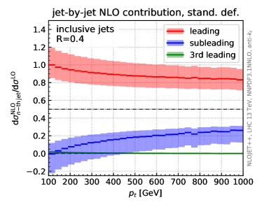
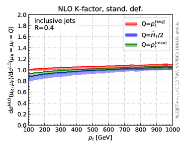
Figure 1: Left: Contributions from the leading, subleading, and third-leading jet to the NLO inclusive cross-section, with central scale choice $\mu_{R}=\mu_{F}=p_{t}^{\text{(avg)}}$ Eq. (9). Right: Inclusive NLO $K$ factors, with three different central scale choices (see text).

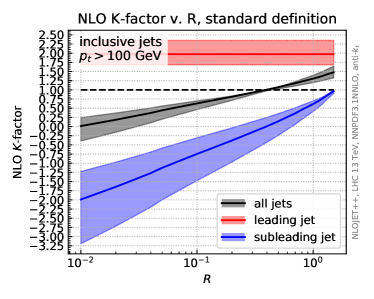
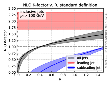
Figure 2: The NLO $K$ factor for the single-inclusive total jet cross-section as a function of the radius $R$ of the jet (black). The contributions from the leading jet (red) and the subleading jet (blue) are also shown. Results are plotted both with a logarithmic (left) and linear (right) scale.

They are shown in Fig. 1 for the standard definition. Three main features are apparent. First, while the total NLO $K$ factor is quite close to one (see the right plot in Fig. 1), the individual $K_{n}$ for the leading and subleading jet deviate from their leading order value, $1/2$, by sizable amounts (see the left plot in Fig. 1). However, they almost exactly compensate when added up into the total cross-section, yielding a total NLO $K$ factor close to 1, as well as a scale uncertainty much smaller than those of the individual $K_{n}$. This almost exact compensation is largely accidental as it depends on the value of the jet radius. This can be seen in Fig. 2, where we plot the $K$ factor for the total cross-section as a function of $R$: the leading and the second leading jet $K$ factors only compensate (up to a residual $\sim 10\%$ effect) in the region $R\sim 0.3-0.6$. This effect has also been noticed in Refs. Dasgupta:2016bnd ; Bellm:2019yyh .

The behavior of the individual jet $K$ factors can be explained in a simple fashion. At NLO, the $K$ factor of the leading jet $K_{1}$ is substantially larger than one, most likely a consequence of recoil effects amplified by the fact that the LO cross-section is steeply falling — typically with a power around 5 — in $p_{t}$. Furthermore, at NLO, $K_{1}$ does not depend on $R$, as explicitly visible in Fig. 2 and as we show analytically in Sect. 4.1 below. However $K_{2}$ decreases at small $R$ since out-of-cone final state radiation depends on the jet radius and has the effect of lowering the $p_{t}$ of the emitter. This effect is again drastically enhanced by the steeply-falling nature of the LO differential cross-section in $p_{t}$.

It can be seen from the logarithmic scale that the dependence of the cross-section on $\ln R$ becomes linear only for $R\mathrel{\hbox to0.0pt{\lower 4.0pt\hbox{\hskip 1.0pt$\sim$}\hss}\raise 1.0pt\hbox{$<$}}0.2$: hence, the logarithmic contribution dominates the cross-section only in the very small $R$ region, and indeed resummation was shown to be necessary in this region in Refs. Dasgupta:2016bnd ; Kang:2016mcy; Liu:2017pbb. For larger $R$ the $\ln R$ term is still sizable, but the bulk of the $\ln R$ effects is captured by the exact NLO result, and for $R\mathrel{\hbox to0.0pt{\lower 4.0pt\hbox{\hskip 1.0pt$\sim$}\hss}\raise 1.0pt\hbox{$>$}}0.4$ there is a modest benefit in resumming them, as also shown in Refs. Dasgupta:2016bnd ; Kang:2016mcy; Liu:2017pbb, where this resummation was performed explicitly.

Second, while the leading and second jet account for most of the cross-section, the contribution of the third jet to the total $K$ factor is much smaller (giving a correction of less than 2% of the LO cross-section) and almost completely negligible. The dominance of the first two jets as $p_{t}$ grows is important in determining the qualitative features of the standard definition, in comparison to the various other definitions that we consider below. It persists at NNLO, as shown in Ref. Currie:2018xkj , and it is in fact to be expected to persist to all orders, as a consequence of the dominance of soft radiation which, combined with the transverse-momentum conservation, favours configurations in which two hard jets are back-to-back while all the others are softer.

Finally, by inspecting the uncertainty bands shown in Fig. 1, one can see that scale variation bands for $R=0.4$ for different central scale choices do not overlap in the small $p_{t}$ region. An in-depth discussion of this problem and how this changes when including even higher order QCD corrections is given in Ref. Currie:2018xkj . It is however clear that this is a consequence of the accidental compensation of the two leading jets discussed above, which then propagates onto the scale variation. It follows that theoretical uncertainties obtained by performing standard scale variation for fixed $R\sim 0.4$ are unrealistically small. A more reliable estimate can be obtained performing uncorrelated scale variation Dasgupta:2016bnd ; Bellm:2019yyh , which then leads to overlapping scale uncertainties across the whole $p_{t}$ spectrum, analogously to what happens in the context of jet vetoing, where decorrelated scale variation also leads to more realistic uncertainty estimates in the presence of cancellations Stewart:2011cf.

All this shows that the putative perturbative instability of the standard definition is in fact a byproduct of an entirely accidental cancellation which happens only at NLO in a given $R$ range. Because this cancellation is not protected by a symmetry, one should not expect it to persist with a different definition or at higher perturbative orders.

3.2 Weighted (unitary) definitions

We now turn to the study of the weighted (unitary) definitions of the single inclusive-jet cross-section introduced in Sect. 2. We start our discussion with case (A), in which a $p_{t}^{\text{cut}}$ is adopted, and we show that in fact this unitary definition appears to display a somewhat problematic behavior, whose origin is discussed analytically in Sect. 4. We then turn to cases (B) and (C) which provide a natural way to alleviate this problematic behavior.

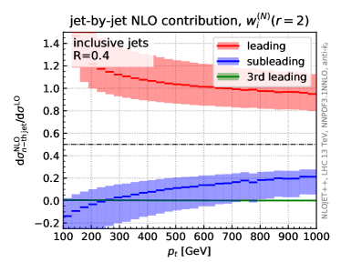
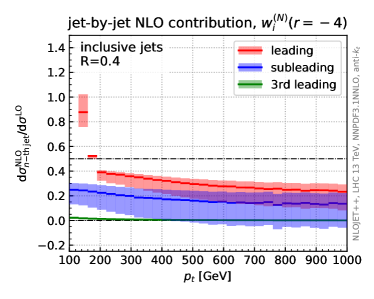
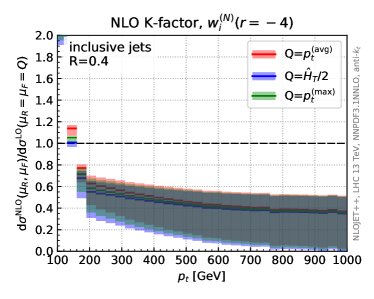
Figure 3: Same as Fig. 1 but using the weighted definitions of type A (see text: jets above $p_{t}^{\text{cut}}$) for $r=2$ (top) and $r=-4$ (bottom).

A. Jets above $p_{t}^{\text{cut}}$.

In Fig. 3 we show again the individual jet contributions and $K$ factor, now using weighted definitions of type (A), with a positive ($r=2$) and a negative ($r=-4$) value for the exponent in the weights. Note that the $K_{n}$, and hence the total $K$ factor, are normalized to the LO weighted jet cross-section which is exactly half of the LO jet cross-section obtained with the standard definition. Indeed, at LO we have $w_{1}=w_{2}=1/2$, by kinematic constraint, for the weighted definition, independently of $r$.

We first discuss the behaviour for $p_{t}$ far above $p_{t}^{\text{cut}}$. Broadly speaking, positive weights enhance the difference between leading and second leading jets, with features that resemble those of the standard definition for the individual $K_{n}$ factors. This is also true, in particular, for the total $K$ factor for $p_{t}$ sufficiently larger than $p_{t}^{\text{cut}}$ (top row of Fig. 3). Negative values of $r$, on the other hand, have the effect of balancing the difference between leading and subleading jets. This results in more similar individual $K_{n}$ factors, at the price of an overall larger total $K$ factor (bottom row of Fig. 3). At very large $p_{t}$ this effect becomes very large, which can be easily understood as follows: whenever we have three jets passing the $p_{t}$ cut with $p_{t1,2}\gg p_{t3}$ we have

$$w_{1,2}^{(3)}(r<0) =\frac{p_{t1,2}^{r}}{p_{t1}^{r}+p_{t2}^{r}+p_{t3}^{r}}\sim\left(\frac{p_{t3}}{p_{t1,2}}\right)^{|r|}\ll 1\,,$$ (12)

$$w_{3}^{(3)}(r<0) =\frac{p_{t3}^{r}}{p_{t1}^{r}+p_{t2}^{r}+p_{t3}^{r}}\sim 1\,.$$ (13)

The contributions of the two leading jets to the inclusive cross-section, which are strongly dominating the NLO cross-section for the standard definition (or for the weighted definition with $r\geq 0$), are now power suppressed by the weights. Furthermore, corresponding virtual corrections have two jets in the final state with $w_{1,2}^{(2)}(r<0)=1/2$. At large $p_{t}$ real and virtual corrections with $p_{t}^{\text{cut}}\ll p_{t3}\ll p_{t1,2}\sim p_{t}$ therefore yield, after integration over $p_{t3}$, a negative contribution enhanced by $\log(p_{t}/p_{t}^{\text{cut}})$, corresponding to the large corrections seen in Fig. 3.

Now turning to the region where $p_{t}\to p_{t}^{\text{cut}}$, we see from Fig. 3 that this weighted definition (for both positive and negative $r$) develops a singular behavior. The origin of this behavior is explained analytically in Section 4. For the time being, we note that these singularities, both for $p_{t}\gg p_{t}^{\text{cut}}$ and for $p_{t}\to p_{t}^{\text{cut}}$, are of logarithmic origin and could in principle be dealt with resummation.

In summary, the weighted definitions of type (A) (with $p_{t}^{\text{cut}}$) have the undesirable feature of developing problematically unstable behaviors for $p_{t}$ close to the $p_{t}$ cut as well as at large $p_{t}$ for $r<0$. In the other $p_{t}$ regions their perturbative behavior now shows large $K$ factors also at NLO since the accidental cancellation of the standard definition is spoiled; while this is perhaps more natural, it does not suggest an improvement in perturbative behavior over the standard definition.

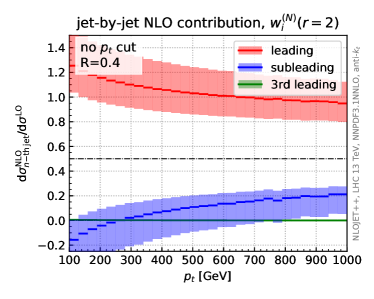
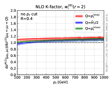
Figure 4: Same as Fig. 1, but using a weighted definition of type B (all jets) for $r=2$.

B. All jets.

A natural way of curing the logarithmic divergence observed when $p_{t}\to p_{t}^{\text{cut}}$ using weights of type (A) is to include all jets down to a $p_{t}$ much smaller than the first bin of the distribution. Based on Fig. 3, taking a $p_{t}^{\text{cut}}$ two or three times smaller than the first bin of the distribution would already get rid of most of the sensitivity to $p_{t}^{\text{cut}}$, e.g. without any need for an additional resummation. One can view the weighted definition of type (B) as simply taking the limit $p_{t}^{\text{cut}}\to 0$ and one should not expect our conclusions to change as long as $p_{t}^{\text{cut}}$ remains much smaller than the first bin of the distribution, say $p_{t}^{\text{cut}}\sim 20-30$ GeV. This possibility is only sensible for positive weights, for which the low $p_{t}$ part of the spectrum is suppressed. For negative weights this choice is infrared unsafe.

Results are shown in Fig. 4 for $r=2$. As expected, the singular behavior of the $K$ factor for $p_{t}$ close to $p_{t}^{\text{cut}}$ is now absent, and features similar to those of the standard definition are now recovered. Specifically, non-overlapping scale variation bands are observed in the low $p_{t}$ region, though to a smaller extent than in the standard case. As a last comment, we have checked that this definition does not suffer from large non-perturbative corrections, such as those coming from underlying events, despite involving low-$p_{t}$ jets. In a practical experimental context, one would still need to make sure that this remains true with realistic pileup conditions.

C. Two leading jets.

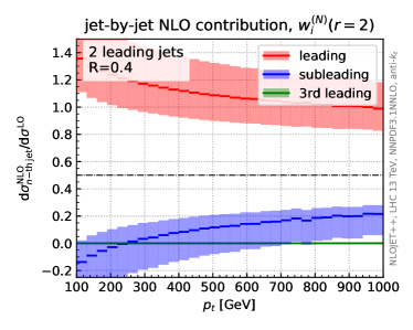
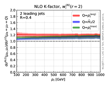
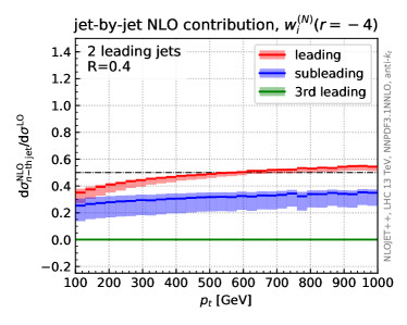
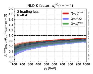
Figure 5: Same as Fig. 1, but using the weighted definitions of type C (two leading jets) for $r=2$ (top) and $r=-4$ (bottom).

An alternative choice, motivated by the observation that the contribution of the third jet to the inclusive jet cross-section is much smaller than that of the first two jets (see Fig. 1) is to switch to definitions of type (C), in which only the two leading jets are included in the weights, whether or not they pass a given $p_{t}^{\text{cut}}$. Clearly this should also remove the problem of the behavior for $p_{t}\sim p_{t}^{\text{cut}}$ of definitions of type (A). This approach is similar in spirit to what is done when looking at the dijet cross-section. Results in this case are presented in Fig. 5 for the individual $K$ factors $K_{n}$ and the total $K$ factor. The situation for positive $r$ is again similar to what we observe for the standard definition: in particular there seems to be a large compensation between the leading and subleading jets, leading to a rather flat $K$ factor, though larger than in the standard case.

As explained above, negative values of $r$ have the effect of normalizing the individual $K_{n}$ factors for the leading and subleading jets, reducing the effect of the compensation seen in the standard case. Furthermore, the uncertainty bands obtained for the three different scale choices now overlap. Nevertheless, the inclusive $K$ factor is relatively larger than for the standard definition and shows a somewhat strong $p_{t}$ dependence.

Comparing these results to the other weighted definitions, we see that the logarithmic divergence for $p_{t}$ close to $p_{t}^{\text{cut}}$ which is observed in Fig. 3 when using the jets above $p_{t}^{\text{cut}}$ has now disappeared for both positive and negative $r$. This, as discussed above, is expected: the weights do not depend on whether one or two of the two leading jets passes the $p_{t}^{\text{cut}}$, so the definition becomes independent of the cut. Furthermore, the issue with large $K$ factors at large $p_{t}$ for negative $r$ when including jets above $p_{t}^{\text{cut}}$ has also disappeared. This is simply because the third jet no longer contributes to the weights and therefore the large contribution seen in Eq. (12) is absent.

In summary, weighted definitions of type (C) behave similarly to the standard definition for positive $r$. The perturbative behavior for negative $r$ changes, with some desirable features (the individual $K$ factors $K_{1}$ and $K_{2}$ are similar, and the scale uncertainty bands for different scale choices overlap), and some undesirable ones (the overall $K$ factor is larger).

4 Non-unitarity and perturbative behavior

We now show how several features of the results presented in the previous section can be understood on the basis of simple analytic arguments. Specifically, we show that the behavior in the vicinity of $p_{t}^{\text{cut}}$ is strongly tied to the unitarity, or lack thereof, of the various definitions.

We first provide general (if somewhat formal) arguments, exploiting the fact that at NLO the jet functions used for partitioning the phase-space have a compact and manageable form. We then perform more explicit calculations using a soft and collinear approximation which shows that the effects discussed in Section 3.2 have a simple leading logarithmic origin.

4.1 Dependence on $p_{t}^{\text{cut}}$ and $R$: a general argument

In order to understand the behavior of various definitions we need an explicit expression for the contribution to the $N$-jet cross-section $\frac{d\sigma^{(k)}_{\text{N\,jet}}}{dp_{t}}$ introduced in Eq. (7) and to the $n$-th jet cross-section $\frac{d\sigma^{(k)}_{\text{n-th\,jet}}}{dp_{t}}$ introduced in Eq. (8). These can be constructed in terms of parton-level cross-sections by introducing explicit jet functions that cluster final-state partons into jets, in the latter case further supplemented by a function that selects the $n$-th leading jet, and bins the result into a fixed $p_{t}$ bin. In order to cancel infrared singularities, the $k$-th order contribution must be constructed by adding up contributions coming from final states with a number of final-state partons that goes from two (with $k$ virtual loops), up to $k+2$ (with $k$ real emissions on top of the Born level). For instance the NLO $k=1$ term receives contributions both from a two-parton final state with one loop, and from a real emission three-parton state, and so on.

Explicitly, we can write the $N$-exclusive jets contribution, Eq. (7), as a sum of terms where the $N$ jets are produced from an $m$ parton final-state, ${\rm d}\Phi_{m}$,

$$\frac{{\rm d}\sigma^{(k)}_{N\,\text{jets}}}{{\rm d}p_{t}}=\sum_{m=2}^{k+2}\int{\rm d}{\Phi}_{m}\frac{{\rm d}\hat{\sigma}^{(k)}_{m}}{{\rm d}{\Phi}_{m}}G_{m\to{N\,\text{jets}}}({\Phi}_{m},p_{t})\,,$$ (14)

where $G_{m\to{N\,\text{jets}}}$ is the jet function which cluster $m$ partons into $N$ jets. $G_{m\to{N\,\text{jets}}}$ contains the function $F_{N}$, Eq. (4), which in turn includes the possible weights. The jet function thus depends on the jet momentum $p_{t}$, and on the partonic phase space variables ${\rm d}\Phi_{m}$.

We can give an explicit expression of $G_{m\to N}$ at NLO ($k=1$). For this, let us denote by $k_{ti}$ the parton transverse momenta, with $k_{t{1}}\geq k_{t{2}}\geq k_{t{3}}$. Using the anti-$k_{t}$ Cacciari:2008gp jet clustering with $R<\tfrac{\pi}{2}$, one has

$$G_{2\to 1} =G_{2\to 3}=0$$ (15)

$$G_{2\to 2} =\Theta(p_{t}>p_{t}^{\text{cut}})\left\{2\,w^{(2)}(p_{t};p_{t},p_{t})\,\delta(p_{t}-k_{t{1}})\right\}$$ (16)

$$G_{3\to 1} =\Theta(\Delta R_{23}>R)\,\Theta(k_{t{1}}>p_{t}^{\text{cut}}>k_{t{2}}>k_{t{3}})\left\{w^{(1)}(p_{t};p_{t})\,\delta(p_{t}-k_{t{1}})\right\}$$ (17)

$$G_{3\to 2} =\Theta(\Delta R_{23}>R)\,\Theta(k_{t{1}}>k_{t{2}}>p_{t}^{\text{cut}}>k_{t{3}})\left\{\sum_{i=1}^{2}w^{(2)}(p_{t};k_{t{1}},k_{t{2}})\,\delta(p_{t}-k_{t{i}})\right\}$$

$$+\Theta(\Delta R_{23}<R)\,\Theta(p_{t}>p_{t}^{\text{cut}})\,\left\{2\,w^{(2)}(p_{t};p_{t},p_{t})\,\delta(p_{t}-k_{t{1}})\right\}$$ (18)

$$G_{3\to 3} =\Theta(\Delta R_{23}>R)\,\Theta(k_{t{1}}>k_{t{2}}>k_{t{3}}>p_{t}^{\text{cut}})\left\{\sum_{i=1}^{3}w^{(3)}(p_{t};k_{t{1}},k_{t{2}},k_{t{3}})\delta(p_{t}-k_{t{i}})\right\},$$ (19)

where we have defined, as is customary, $\Delta R_{ij}=\sqrt{(\Delta\phi_{ij})^{2}+(\Delta y_{ij})^{2}}$, as the distance between parton $i$ and parton $j$ in the rapidity-azimuth plane, with $y$ and $\phi$ the rapidity and the azimuthal angle respectively. Note also that, due to momentum conservation, it is sufficient to consider the recombination of the two softest partons. The second line of Eq. (18) corresponds to the case where the two softest partons cluster, yielding two back-to-back jets of momentum $k_{t{1}}$.

Using Eqs. (15)-(19), the issue of unitarity vs. cancellation of the dependence on $p_{t}$ is easily understood. On the one hand, it is clear that the standard definition is not unitary and only the weighted definitions are unitary because

$$\int{\rm d}\,p_{t}\,G_{3\to 1}+G_{3\to 2}+G_{3\to 3}\big{|}_{\text{wgt}}=\Theta(k_{t{1}}>p_{t}^{\text{cut}})\,,$$ (20)

This result, valid for any $r$, means that integrating the single-jet cross-section over $p_{t}$ yields the total cross-section for producing (at least) one jet above $p_{t}^{\text{cut}}$ (with definitions of type (A) in the sense of Sect. 2) or the total cross-section (for definitions of type (B) or of type (C)). Hence these choices are unitary, and thus the standard choice cannot be.

On the other hand, it is clear that the inclusive cross-section is independent of $p_{t}^{\text{cut}}$ when using the standard definition. Indeed, in this case one has

$$G_{3\to 1}+G_{3\to 2}+G_{3\to 3}\big{|}_{\text{std}}=\Theta(p_{t}>p_{t}^{\text{cut}})\Bigg{\{}\Theta(\Delta R_{23}>R)\left[\sum_{i}^{3}\delta(p_{t}-k_{t{i}})\right]+\Theta(\Delta R_{23}<R)2\,\delta(p_{t}-k_{t{1}})\Bigg{\}},$$ (21)

where now the subscript “std” denotes that in the definition of $F_{N}$, Eq. (4), the standard case in Eq. (5) has been selected. The result Eq. (21) is manifestly independent of $p_{t}^{\text{cut}}$ since all the dependence on $p_{t}^{\text{cut}}$ is factored in an overall $\Theta$ function which is always satisfied as long as one has at least one jet in the event. In practice, the dependence on $p_{t}^{\text{cut}}$ disappears since, when integrating over the partonic transverse momenta, the $N$-jet contribution has $p_{t}^{\text{cut}}$ as a lower bound of integration while the $N-1$-jet contribution has $p_{t}^{\text{cut}}$ as an upper bound. When summing both contributions, the $p_{t}^{\text{cut}}$ dependence cancels.

When one instead uses a unitary definition which explicitly introduces a $p_{t}^{\text{cut}}$ dependence, such as definition (A), this cancellation is spoiled: whether a jet passes a cut or not changes the weights of all the other jets, thereby introducing a cutoff dependence of the observable. The lack of cancellation then propagates into the individual $n$-th jet cross-sections, thus explaining the singular behavior observed in Fig. 3 when $p_{t}\sim p_{t}^{\text{cut}}$. Of course this cutoff dependence is not present for the two other weighted definitions, (B) and (C), even if the weight associated to a jet still depends on the other jets in the event, which is needed to eventually ensure the unitarity of the cross-section.

We can similarly understand the $R$ dependence or lack thereof of the leading jet contribution, which as discussed in Sect. 3.1 controls the behavior of the NLO $K$ factor, by introducing explicit expressions for individual jet functions. We now need to consider the $n$-th leading jet contribution, Eq. (8)

$$\frac{{\rm d}\sigma^{(k)}_{n\text{-th\,jet}}}{{\rm d}p_{t}}=\sum_{m=2}^{k+2}\int{\rm d}{\Phi}_{m}\frac{{\rm d}\hat{\sigma}^{(k)}_{m}}{{\rm d}{\Phi}_{m}}S_{m\to{n\text{-th jet}}}({\Phi}_{m},p_{t})\,,$$ (22)

where the functions $S_{m\to{n\text{-th jet}}}$ are defined summing the contributions coming from the $n$-th jet in the functions $G$ given above. By direct calculation, we find

$$S_{2\to p_{t1}} =S_{2\to p_{t2}}=\frac{1}{2}\,G_{2\to 2}$$ (23)

$$S_{3\to p_{t1}} =\Theta(p_{t}>p_{t}^{\text{cut}})\,\delta(p_{t}-k_{t{1}})\,\biggl{\{}\Theta(\Delta R_{23}>R)\,\Bigl{[}\Theta(p_{t}^{\text{cut}}>k_{t{2}}>k_{t{3}})w^{(1)}(p_{t};k_{t{1}})$$

$$\hphantom{=\Theta(p_{t}>p_{t}^{\text{cut}})\,\delta(p_{t}-k_{t{1}})\,\biggl{\{}\Theta(\Delta R_{23}>R)\,\Bigl{[}}+\,\Theta(k_{t{2}}>p_{t}^{\text{cut}}>k_{t{3}})\,w^{(2)}(p_{t};k_{t{1}},k_{t{2}})$$

$$\hphantom{=\Theta(p_{t}>p_{t}^{\text{cut}})\,\delta(p_{t}-k_{t{1}})\,\biggl{\{}\Theta(\Delta R_{23}>R)\,\Bigl{[}}+\Theta(k_{t{2}}>k_{t{3}}>p_{t}^{\text{cut}})w^{(3)}(p_{t};k_{t{1}},k_{t{2}},k_{t{3}})\Bigr{]}\,$$

$$\hphantom{=\Theta(p_{t}>p_{t}^{\text{cut}})\,\delta(p_{t}-k_{t{1}})\,\biggl{\{}}+\Theta(\Delta R_{23}<R)\,w^{(2)}(p_{t};p_{t},p_{t})\biggr{\}}$$ (24)

$$S_{3\to p_{t2}} =\Theta(k_{t{1}}>p_{t}>p_{t}^{\text{cut}})\biggl{\{}\Theta(\Delta R_{23}>R)\,\delta(p_{t}-k_{t{2}})\Bigl{[}\Theta(p_{t}^{\text{cut}}>k_{t{3}})\,w^{(2)}(p_{t};k_{t{1}},k_{t{2}})$$

$$\hphantom{=\Theta(k_{t{1}}>p_{t}>p_{t}^{\text{cut}})\biggl{\{}\Theta(\Delta R_{23}>R)\,\delta(p_{t}-k_{t{2}})\Bigl{[}}+\Theta(k_{t{3}}>p_{t}^{\text{cut}})\,w^{(3)}(p_{t};k_{t{1}},k_{t{2}},k_{t{3}})\Bigr{]}\,$$

$$\hphantom{=\Theta(k_{t{1}}>p_{t}>p_{t}^{\text{cut}})\biggl{\{}}+\Theta(\Delta R_{23}<R)\,\delta(p_{t}-k_{t{1}})\,w^{(2)}(p_{t};p_{t},p_{t})\biggr{\}}$$ (25)

$$S_{3\to p_{t3}} =\Theta(k_{t{1}}>k_{t{2}}>p_{t}>p_{t}^{\text{cut}})\,\delta(p_{t}-k_{t{3}})\,\Theta(\Delta R_{23}>R)\,w^{(3)}(p_{t};k_{t{1}},k_{t{2}},k_{t{3}})\,.$$ (26)

If now one sets all weights $w=1$, Eq. (24) takes the form

$$S_{3\to p_{t1}}\big{|}_{\text{std}}=\Theta(p_{t}>p_{t}^{\text{cut}})\,\delta(p_{t}-k_{t{1}})=S_{2\to p_{t1}}\big{|}_{\text{std}}\,,$$ (27)

where the subscript “std” again denotes that in the definition of $F_{N}$, Eq. (4), the standard case in Eq. (5) has been selected. This means that all the $\Theta$ functions simplify, leading to an overall factor providing a condition that is always satisfied if at least one jet in the event is above $p_{t}^{\text{cut}}$. At NLO, the leading jet contribution is therefore always given by the transverse momentum of the hardest parton (this is valid for both the real contribution with three partons in the final state and the virtual corrections with two partons), independently of the jet radius $R$. Note that, one can similarly see that for any weighted definition, at NLO, corrections to the leading jet are $R$-dependent for the same reason that the weighted definitions depend on $p_{t}^{\text{cut}}$: the value of the weights depend on how many partons have $\Delta R_{ij}>R$. Furthermore, the NLO corrections for the subleading and third-leading jet also depend on $R$. This is trivial for the latter which shows an explicit $R$ dependence in (26). For the subleading jet, this is due to the fact that the $p_{t}$ of the jet changes (between $k_{t{1}}$ and $k_{t{2}}$) depending on how $\Delta R_{23}$ compares to $R$.

4.2 Dependence on $p_{t}^{\text{cut}}$ and $R$: the soft-collinear approximation

The arguments outlined above may seem somewhat formal. To gain further analytic insight, it is useful to take a soft-collinear approximation in which case Eqs. (14),(22) simplify considerably. Indeed, if one considers a collinear splitting at a small angle $\vartheta$, the NLO contribution from a real emission can be written in simple form by parametrising the final-state momenta as

$$p_{1}^{\mu}=\tilde{p}_{a}^{\mu}+\mathcal{O}(k_{\perp}^{2}),\quad p_{2}^{\mu}=(1-z)\tilde{p}_{b}^{\mu}+k_{\perp}^{\mu}+\mathcal{O}(k_{\perp}^{2}),\quad p_{3}^{\mu}=z\,\tilde{p}_{b}^{\mu}-k_{\perp}^{\mu}+\mathcal{O}(k_{\perp}^{2}),$$ (28)

where $\tilde{p}_{a}^{\mu}$ and $\tilde{p}_{b}^{\mu}$ are the Born final-state hard directions, $z$ is the longitudinal momentum fraction of the splitting, and the transverse momentum $k_{\perp}$ satisfies $k_{\perp}\cdot\tilde{p}_{a}=k_{\perp}\cdot\tilde{p}_{b}=0$; $k_{\perp}$ can then be parametrized by the angle $\vartheta$ between $p_{2}$ and $p_{3}$ and an azimuthal angle $\varphi$.

Including only terms that produce a logarithmic enhancement in the limit $\vartheta\to 0$, the real emission contribution takes the form

$$d{\Phi}_{3}\frac{d\hat{\sigma}^{(1)}_{3}}{d{\Phi}_{3}}=\sum_{i=q,g}\left[\frac{d\sigma^{(0)}_{2}}{dp_{t}}(\tilde{p}_{t})\right]_{i}\left[\frac{\alpha_{s}C_{i}}{\pi}P_{i}(z)\right]\,{\rm d}\tilde{p}_{t}\,{\rm d}z\frac{{\rm d}\vartheta^{2}}{\vartheta^{2}}\frac{d\varphi}{2\pi}.$$ (29)

Note that within this approximation recoil effects on $p_{1}$ become negligible. They could be addressed using a similar formalism but going beyond the small-angle approximation that we adopt here.

In Eq. (29) $[d\sigma^{(0)}_{2}/dp_{t}]_{i}$, with $i=q,g$, is the LO differential cross-section for producing a quark or a gluon of transverse momentum $\tilde{p}_{t}$, correctly normalized in such a way that the sum over $i$ gives the total cross-section. $P_{i}(z)$ corresponds to the standard Altarelli-Parisi splitting functions with $z$ the momentum fraction of the collinear splitting (see Appendix A for explicit expressions) from which we have explicitly factored out a colour factor $2\,C_{i}$ ($C_{i}=C_{F}$ for quarks and $C_{i}=C_{A}$ for gluons). Finally, $\varphi$ is the azimuthal angle corresponding of the emission with respect to the Born-level parton that splits. At this accuracy, the NLO one-loop virtual correction has exactly the same form as Eq. (29) integrated over the full phase-space of the extra real emission, but with the opposite sign. In what follows, we further assume that the extra emission is soft so we can approximate $P_{i}(z)\approx\frac{1}{z}$. This soft approximation is made for the sake of simplicity and can easily be lifted to include the full splitting function.

The soft-collinear approximation is sufficient to obtain results in fair agreement with the full calculation, and specifically reproduce three important aspects discussed in Sect. 3. First, we can see explicitly how the cancellation of the $p_{t}^{\text{cut}}$ dependence which happens in the standard case is spoiled for the weighted definition (A) and restored with definitions (B) and (C). Second, we are able to identify the $R$ dependence of the second leading jet with out-of-cone radiation. Third, we can further study the impact of weighted definitions at large $p_{t}$. Conversely, working in a soft-collinear approximation, we are neglecting all recoil effects. This means in particular that the calculation below will not reproduce the large $K_{1}$ factor for the leading jet. The text below outlines the structure of the calculation and our main results, deferring additional details to Appendix A.

The fact that the real and virtual contributions have the opposite sign implies that the $N$-jet contribution Eq. (14) and the $n$-th jet contribution Eq. (22) take respectively the simple form

$$\frac{d\sigma^{(k)}_{N\,\text{jets}}}{dp_{t}} \approx\sum_{i=q,g}\frac{C_{i}}{\pi}\int{\rm d}\tilde{p}_{t}\,{\rm d}z\frac{{\rm d}\vartheta^{2}}{\vartheta^{2}}\left[\frac{d\sigma^{(0)}_{2}}{dp_{t}}(\tilde{p}_{t})\right]_{i}\alpha_{s}\,P_{i}(z)\,\left\{G_{3\to{N\,\text{jets}}}-G_{2\to{N\,\text{jets}}}\right\}$$ (30)

$$\equiv\sum_{i=q,g}\left[\frac{d\sigma^{(0)}_{2}}{dp_{t}}(p_{t})\right]_{i}\frac{C_{i}}{\pi}\ln\left(\frac{R_{\text{max}}^{2}}{R^{2}}\right)I_{N}$$ (31)

and

$$\frac{d\sigma^{(k)}_{n\,\text{-th jet}}}{dp_{t}} \approx\sum_{i=q,g}\frac{C_{i}}{\pi}\int{\rm d}\tilde{p}_{t}\,{\rm d}z\frac{{\rm d}\vartheta^{2}}{\vartheta^{2}}\left[\frac{d\sigma^{(0)}_{2}}{dp_{t}}(\tilde{p}_{t})\right]_{i}\alpha_{s}\,P_{i}(z)\,\left\{S_{3\to{n\,\text{-th jet}}}-S_{2\to{n\,\text{-th jet}}}\right\}$$ (32)

$$\equiv\sum_{i=q,g}\left[\frac{d\sigma^{(0)}_{2}}{dp_{t}}(p_{t})\right]_{i}\frac{C_{i}}{\pi}\ln\left(\frac{R_{\text{max}}^{2}}{R^{2}}\right)J_{n}\,,$$ (33)

where in both cases $R_{\text{max}}$ is the upper limit of the $\vartheta$ integration. The functions $I_{N}$ and $J_{n}$ can be cast in a simple closed analytic form by writing the LO cross-section as a power law

$$\left[\frac{d\sigma^{(0)}_{2}}{dp_{t}}(\tilde{p}_{t})\right]_{i}\sim\frac{1}{\tilde{p}_{t}^{m_{i}}},$$ (34)

where $m_{i}$ is, in general, different for the quark and gluon case. In Appendix A explicit analytic expressions are given for the standard definition, with the general definitions easily amenable to numerical treatment.

We can now use Eqs. (31),(33) to address the issues mentioned above. We start by investigating the behavior in the $p_{t}\rightarrow p_{t}^{\text{cut}}$ limit and focus on the leading jet. $J_{1}$ receives real contributions from $S_{3\to p_{t1}}$, Eq. (24), and virtual corrections from $S_{2\to p_{t1}}$, Eq. (23). The latter contribution cancels against the real one in the region $\Delta R_{23}\equiv\vartheta<R$. Up to power corrections in $z$, we can set $k_{t{2}}=(1-z)k_{t{1}}$ and $k_{t{3}}=zk_{t{1}}$. For $p_{t}\to p_{t}^{\text{cut}}$ we can then assume $k_{t{3}}<p_{t}^{\text{cut}}$ and we are left with two terms:

$$J_{1}\stackrel{{\scriptstyle p_{t}\to p_{t}^{\text{cut}}}}{{\sim}}\int_{1-p_{t}^{\text{cut}}/p_{t}}^{p_{t}^{\text{cut}}/p_{t}}dz\,P(z)\,w^{(1)}(p_{t};p_{t})-\int_{1-p_{t}^{\text{cut}}/p_{t}}^{p_{t}^{\text{cut}}/p_{t}}dz\,P(z)\,w^{(2)}(p_{t};p_{t},p_{t}).$$ (35)

The first term corresponds to $k_{t{2}}<p_{t}^{\text{cut}}$ while the second term includes the real emissions with $k_{t{2}}>p_{t}^{\text{cut}}$ as well as the remaining virtual corrections. After integration over $z$, we thus find

$$J_{1}=\log\left(\frac{p_{t}^{\text{cut}}}{p_{t}-p_{t}^{\text{cut}}}\right)-\omega\log\left(\frac{p_{t}^{\text{cut}}}{p_{t}-p_{t}^{\text{cut}}}\right)=\begin{cases}0&\,({\text{standard}})\\ -\frac{1}{2}\log\left(\frac{p_{t}-p_{t}^{\text{cut}}}{p_{t}^{\text{cut}}}\right)&\,({\text{weighted (A)}})\end{cases}\,,$$ (36)

where $\omega=1$ for the standard definition and $\omega=\tfrac{1}{2}$ for the weighted definition (A), independently of the exponent $r$ which enters the definition of the weights, Eq. (4). In the same limit it turns out that $J_{2}$ and $J_{3}$ are nonsingular. This explains our findings from Sect. 3: the unitary definition suffers from a logarithmic divergence close to $p_{t}^{\text{cut}}$ while the standard definition is independent of the value of $p_{t}^{\text{cut}}$. Furthermore, this behavior (see Fig. 3), only affects the leading jet, whose properties are encoded in $J_{1}$. Of course it also follows from Eq. (36) that when $p_{t}^{\text{cut}}\ll p_{t}$, corresponding to using definitions of the weights of type (B), the singular behavior disappears. A similar conclusion can be reached for the definition of type (C).

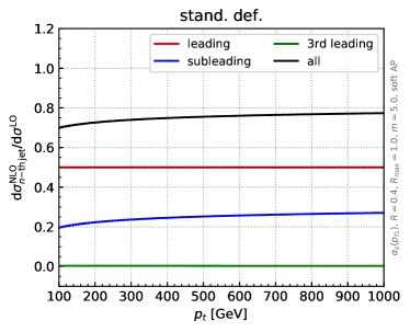
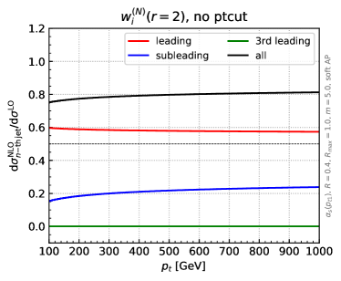
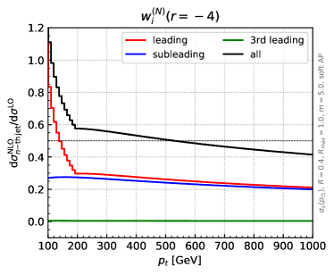
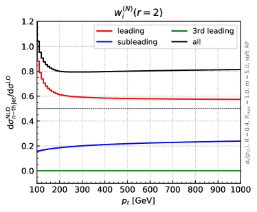
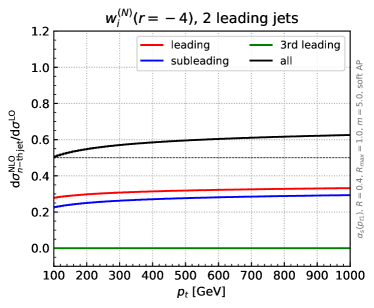
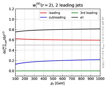
Figure 6: Contributions from the leading, subleading, and third-leading jets to the NLO inclusive $K$ factors in the soft-collinear approximation. The standard definition (top left) is compared to weighted definition of type (B) (no $p_{t}^{\text{cut}}$) with $r=2$ (top right), weighted definitions of type (A) (with $p_{t}^{\text{cut}})$ with $r=-4$ (middle left) and $r=2$ (middle right) and of type (C) (two jets) also with with $r=-4$ (bottom left) and $r=2$ (bottom right).

Next, we can also use Eq. (33) to predict the small-$R$ behavior of the second and third leading jet contributions. In both cases one would get a logarithmic enhancement at small $R$. Note that at first sight Eq. (33) seems to imply that the leading jet contribution also has a logarithmic $R$ dependence in the standard case, in contradiction to the behavior observed in Fig. 2, and to our previous general conclusion based on Eq. (27). However, one should realise that, in the small-$R$ limit where Eq. (33) holds, Eq. (36) implies that $J_{1}$ is zero, and thus obviously $R$-independent in the standard case. In all weighted cases $J_{1}$ is non-vanishing, and thus the leading jet contribution becomes $R$-dependent in agreement with our previous analytic and numerical arguments, with a logarithmic dependence on $R$ in the small-$R$ limit.

Finally, we can study the limit of the functions $J_{n}$ when $p_{t}\gg p_{t}^{\text{cut}}$, in the weighted case with $r$ negative and $|r|\sim|m_{i}|\sim 4$. In this case, we find that the contributions from the leading and the subleading jet are comparable (see the Appendix A for details), partially solving the problem of the large compensation seen in the standard definition or for positive values of $r$, as observed in Sect. 3.2, Fig. 3.

Results obtained for the leading, subleading and third-leading jet contributions using the approximation Eqs. (31),(33) are shown in Fig. 6 for a representative set of cases, to be compared to Figs. 1,3-5. All plots have been produced implementing Eq. (32), with Eq. (34) and $m=5$. Note that this parametrization of the LO $p_{t}$ spectrum already includes initial state PDFs. We have checked that using the exact LO partonic cross-section yields similar results. We choose $R_{\text{max}}=1$ and use $R=0.4$ to allow for a comparison with the full results presented in Section 3. Finally, we set $\alpha_{s}(p_{t1})$. As anticipated, it is clear that the main qualitative features of the exact results are reproduced by the soft-collinear approximation.

5 Conclusions

Definition	standard	weighted
		(A) above $p_{t}^{\text{cut}}$	(B) all jets	(C) two leading
Reference plot	Fig. 1	Fig. 3	Fig. 4	Fig. 5
unitarity	no	yes	yes	yes
no large logs	$\checkmark$	✗	$\checkmark$	$\checkmark$
close to $p_{t}^{\text{cut}}$
no large logs	$\checkmark$	$\checkmark$ for $r>0$	$\checkmark$	$\checkmark$
at large $p_{t}$		✗ for $r<0$
overlapping scale	✗	$\checkmark$	$\checkmark$	$\checkmark$
variation bands	$\checkmark$ with uncorr. uncert. Dasgupta:2016bnd ; Currie:2016bfm
no large cancellations	✗	✗	✗	✗ for $r>0$
between $K_{1}$ and $K_{2}$				$\checkmark$ for $r<0$

Table 1: Summary of the main properties of the various single-inclusive jet definitions studied in this paper.

In this paper we have addressed the potential issue of the non-unitarity of the single-jet inclusive cross-section, by introducing a series of alternative weighted definitions of this observable which are unitary in the sense that upon integration they lead to the total cross-section. The main features of the various definitions we have considered are summarised in Table 1.

Our conclusion is that a naive weighted approach [type (A) of Sect. 2] in which one simply introduces a weighting of all jets above a certain $p_{t}^{\text{cut}}$ is flawed, in the sense that it develops logarithmic singularities associated with the transverse momentum cut on jets, $p_{t}^{\text{cut}}$. More sophisticated definitions avoid this problem by setting $p_{t}^{\text{cut}}$ to zero [type (B)] or by considering only the two leading jets [type (C)]. Both these definitions could be more challenging to implement in a practical (experimental) environment.

Additionally, even leaving aside practical considerations, there does not seems to be any real advantage in adopting these definitions in term of perturbative stability. In particular, all weighted definitions with positive $r$ show features at best similar to the standard definition. Furthermore, the apparent perturbative instability of the conventional definition appears in fact to be the manifestation of an unnatural smallness of the NLO $K$ factors which only happens for a limited range of jet radius $R\sim 0.4$. It is a consequence of an accidental cancellation which makes standard scale variation unreliable as a means of estimating missing higher order corrections. This apparent issue for example disappears with more conservative estimates of the perturbative uncertainties. One possible case of interest is the definition of type (C), focusing on the two leading jets, with $r<0$. Compared to the standard definition, it has the potential advantage of reducing the large difference between the $K$ factor of the leading and subleading jets, at the cost of having a larger overall NLO $K$ factor.

Our final conclusion is both negative, and positive. On the negative side, we conclude that unitary definitions of the jet inclusive cross-section are at best as good as the standard definition, while being rather more contrived. On the positive side, we conclude that the standard definition shows no critical sign of pathological features or problems, other than its unitarity, which however is per se not causing any perturbative problem. Among the unitary definitions, the weighted definitions based on including only the two leading jets appear to be particularly well-behaved. While in this work we study the dijet system as a function of the $p_{t}$ and rapidity of the individual jets, this is in agreement with previous studies Currie:2018xkj in which dijet observables are also found to have better perturbative stability.

Appendix A NLO cross-section in the soft-collinear approximation

The $N$-jet contribution and the $n$-th jet contribution to the differential cross-section at NLO in the soft-collinear approximation are given by Eq. (30) and Eq. (32) respectively. Using an explicit expression for the splitting functions $P_{i}$ and for the $G$ or the $S$ functions in the collinear limit we can perform the phase-space integration explicitly.

The splitting functions $P_{i}$ are

$$\begin{split}P_{q}(z)&=\sum_{j=q,g}P_{jq}=\frac{1+(1-z)^{2}}{2z}=\frac{1}{z}+\mathcal{O}(1)\\ P_{g}(z)&=\sum_{j=q,g}P_{jg}=\frac{1}{2}\left[2\frac{1-z}{z}+z(1-z)+\frac{T_{R}N_{f}}{C_{A}}(z^{2}+(1-z)^{2})\right]=\frac{1}{z}+\mathcal{O}(1)\end{split}$$ (37)

where the $z\leftrightarrow(1-z)$ symmetry has been exploited in such a way that all soft-collinear singularities are at $z=0$ (see e.g. jetbook ). Note that a $2C_{F}$ or $2C_{A}$ factor, respectively, has been explicitly factored out.

By adopting the parametrization of the final-state given in Eq. (28), the jet functions $G$ and $S$ can be rewritten in the collinear and small $R$ limit, i.e. $\Delta R_{23}=\vartheta\leq R\ll 1$. For the weighted definition with jets above $p_{t}^{\text{cut}}$ we have:

$$G_{2\to 1} =G_{2\to 3}=0$$ (38)

$$G_{2\to 2} =\Theta(\tilde{p}_{t}>p_{t}^{\text{cut}})w^{(2)}(p_{t}|\tilde{p}_{t},\tilde{p}_{t})[\delta(p_{t}-\tilde{p}_{t})+\delta(p_{t}-\tilde{p}_{t})]$$ (39)

$$G_{3\to 1} =\Theta(\vartheta^{2}>R^{2})\Theta(\tilde{p}_{t}>p_{t}^{\text{cut}};z\tilde{p}_{t}<p_{t}^{\text{cut}};(1-z)\tilde{p}_{t}<p_{t}^{\text{cut}})w^{(1)}(p_{t}|\tilde{p}_{t})[\delta(p_{t}-\tilde{p}_{t})]$$ (40)

$$G_{3\to 2} =\Theta(\vartheta^{2}<R^{2})\Theta(\tilde{p}_{t}>p_{t}^{\text{cut}})w^{(2)}(p_{t}|\tilde{p}_{t},\tilde{p}_{t})[\delta(p_{t}-\tilde{p}_{t})+\delta(p_{t}-\tilde{p}_{t})]$$

$$+\Theta(\vartheta^{2}>R^{2})\Theta(\tilde{p}_{t}>p_{t}^{\text{cut}})$$

$$\phantom{+}\Big{\{}\Theta(z\tilde{p}_{t}<p_{t}^{\text{cut}};(1-z)\tilde{p}_{t}>p_{t}^{\text{cut}})w^{(2)}(p_{t}|\tilde{p}_{t},(1-z)\tilde{p}_{t})[\delta(p_{t}-\tilde{p}_{t})+\delta(p_{t}-(1-z)\tilde{p}_{t})]$$

$$\phantom{+}+\Theta(z\tilde{p}_{t}>p_{t}^{\text{cut}};(1-z)\tilde{p}_{t}<p_{t}^{\text{cut}})w^{(2)}(p_{t}|\tilde{p}_{t},z\tilde{p}_{t})[\delta(p_{t}-\tilde{p}_{t})+\delta(p_{t}-z\tilde{p}_{t})]\Big{\}}$$ (41)

$$G_{3\to 3} =\Theta(\vartheta^{2}>R^{2})\Theta(\tilde{p}_{t}>p_{t}^{\text{cut}};z\tilde{p}_{t}>p_{t}^{\text{cut}};(1-z)\tilde{p}_{t}>p_{t}^{\text{cut}})$$

$$\phantom{==}w^{(3)}(p_{t}|\tilde{p}_{t},z\tilde{p}_{t},(1-z)\tilde{p}_{t})[\delta(p_{t}-\tilde{p}_{t})+\delta(p_{t}-z\tilde{p}_{t})+\delta(p_{t}-(1-z)\tilde{p}_{t})].$$ (42)

and

$$S_{2\to p_{t1}} =S_{2\to p_{t2}}=\Theta(\tilde{p}_{t}>p_{t}^{\text{cut}})w^{(2)}(p_{t}|\tilde{p}_{t},\tilde{p}_{t})\delta(p_{t}-\tilde{p}_{t})$$ (43)

$$S_{3\to p_{t1}} =\Theta(\vartheta^{2}<R^{2})\Theta(\tilde{p}_{t}>p_{t}^{\text{cut}})w^{(2)}(p_{t}|\tilde{p}_{t},\tilde{p}_{t})\delta(p_{t}-\tilde{p}_{t})+\Theta(\vartheta^{2}>R^{2})$$ (44)

$$\quad\Big{[}\Theta(\tilde{p}_{t}>p_{t}^{\text{cut}};z\tilde{p}_{t}<p_{t}^{\text{cut}};(1-z)\tilde{p}_{t}<p_{t}^{\text{cut}})w^{(1)}(p_{t}|\tilde{p}_{t})\delta(p_{t}-\tilde{p}_{t})$$

$$\quad+\Theta(\tilde{p}_{t}>p_{t}^{\text{cut}};z\tilde{p}_{t}>p_{t}^{\text{cut}};(1-z)\tilde{p}_{t}<p_{t}^{\text{cut}})w^{(2)}(p_{t}|\tilde{p}_{t},z\tilde{p}_{t})\delta(p_{t}-\tilde{p}_{t})$$

$$\quad+\Theta(\tilde{p}_{t}>p_{t}^{\text{cut}};z\tilde{p}_{t}<p_{t}^{\text{cut}};(1-z)\tilde{p}_{t}>p_{t}^{\text{cut}})w^{(2)}(p_{t}|\tilde{p}_{t},(1-z)\tilde{p}_{t})\delta(p_{t}-\tilde{p}_{t})$$

$$\quad+\Theta(\tilde{p}_{t}>p_{t}^{\text{cut}};z\tilde{p}_{t}>p_{t}^{\text{cut}};(1-z)\tilde{p}_{t}>p_{t}^{\text{cut}})w^{(3)}(p_{t}|\tilde{p}_{t},z\tilde{p}_{t},(1-z)\tilde{p}_{t})\delta(p_{t}-\tilde{p}_{t})\Big{]}$$

$$S_{3\to p_{t2}} =\Theta(\vartheta^{2}<R^{2})\Theta(\tilde{p}_{t}>p_{t}^{\text{cut}})w^{(2)}(p_{t}|\tilde{p}_{t},\tilde{p}_{t})\delta(p_{t}-\tilde{p}_{t})+\Theta(\vartheta^{2}>R^{2})$$ (45)

$$\quad\Big{\{}\Theta(\tilde{p}_{t}>p_{t}^{\text{cut}};z\tilde{p}_{t}>p_{t}^{\text{cut}};(1-z)\tilde{p}_{t}<p_{t}^{\text{cut}})w^{(2)}(p_{t}|\tilde{p}_{t},z\tilde{p}_{t})\delta(p_{t}-z\tilde{p}_{t})$$

$$\quad+\Theta(\tilde{p}_{t}>p_{t}^{\text{cut}};z\tilde{p}_{t}<p_{t}^{\text{cut}};(1-z)\tilde{p}_{t}>p_{t}^{\text{cut}})w^{(2)}(p_{t}|\tilde{p}_{t},(1-z)\tilde{p}_{t})\delta(p_{t}-(1-z)\tilde{p}_{t})$$

$$\quad+\Theta(\tilde{p}_{t}>p_{t}^{\text{cut}};z\tilde{p}_{t}>p_{t}^{\text{cut}};(1-z)\tilde{p}_{t}>p_{t}^{\text{cut}})w^{(3)}(p_{t}|\tilde{p}_{t},z\tilde{p}_{t},(1-z)\tilde{p}_{t})$$

$$\quad\quad\quad\quad\left[\Theta(z>1/2)\delta(p_{t}-z\tilde{p}_{t})+\Theta(z<1/2)\delta(p_{t}-(1-z)\tilde{p}_{t})\right]\Big{\}}$$

$$S_{3\to p_{t3}} =\Theta(\vartheta^{2}>R^{2})\Theta(\tilde{p}_{t}>p_{t}^{\text{cut}};z\tilde{p}_{t}>p_{t}^{\text{cut}};(1-z)\tilde{p}_{t}>p_{t}^{\text{cut}})w^{(3)}(p_{t}|\tilde{p}_{t},z\tilde{p}_{t},(1-z)\tilde{p}_{t})$$

$$\phantom{=}\left[\Theta(z<1/2)\delta(p_{t}-z\tilde{p}_{t})+\Theta(z>1/2)\delta(p_{t}-(1-z)\tilde{p}_{t})\right]$$ (46)

The standard definition can trivially be recovered by setting the weights to 1, while the case of the weighted definition including all jets can be obtained by taking the limit $p_{t}^{\text{cut}}\to 0$. Similarly, the weighted definition with 2 leading jets is instead obtained by firstly taking the limit $p_{t}^{\text{cut}}\to 0$ and by then keeping the terms proportional to $\delta(p_{t}-\tilde{p}_{t})$ as well as the terms proportional to either $\delta(p_{t}-z\tilde{p}_{t})$ if $z>1/2$, or $\delta(p_{t}-(1-z)\tilde{p}_{t})$ if $z<1/2$, modifying the weights accordingly.

The $\tilde{p}_{t}$ integration in Eqs. (30)-(32) can be simplified using the delta functions $\delta(p_{t}-\tilde{p}_{t})$, $\delta(p_{t}-z\tilde{p}_{t})$ and $\delta(p_{t}-(1-z)\tilde{p}_{t})$. The $\vartheta$ integration leads to a logarithmic dependence on the jet radius $R$. The only nontrivial integral is over $z$, thereby leading to a final result of the form of Eqs. (31),(33). Explicitly, $I_{N}$ and $J_{n}$ there present are given by:

$$I_{1}=\Theta(p_{t}<2p_{t}^{\text{cut}})\int_{1-p_{t}^{\text{cut}}/p_{t}}^{p_{t}^{\text{cut}}/p_{t}}dz\,P(z)\left[1\right]\tilde{\sigma}(p_{t})$$ (47)

$$\begin{split}I_{2}=&\Theta(p_{t}<2p_{t}^{\text{cut}})\Bigg{[}\int_{p_{t}^{\text{cut}}/p_{t}}^{1}dz\,P(z)\left[\frac{1}{1+z^{r}}\right]\tilde{\sigma}(p_{t})\\ &\phantom{=}+\int_{0}^{1-p_{t}^{\text{cut}}/p_{t}}dz\,P(z)\left(\left[\frac{1}{1+(1-z)^{r}}\right]\tilde{\sigma}(p_{t})-\left[\frac{1}{2}\right]\tilde{\sigma}(p_{t})\right)-\int_{1-p_{t}^{\text{cut}}/p_{t}}^{1}dz\,P(z)\left[\frac{1}{2}\right]\tilde{\sigma}(p_{t})\Bigg{]}\\ &+\Theta(p_{t}>2p_{t}^{\text{cut}})\Bigg{[}\int_{1-p_{t}^{\text{cut}}/p_{t}}^{1}dz\,P(z)\left[\frac{1}{1+z^{r}}\right]\tilde{\sigma}(p_{t})\\ &\phantom{=}+\int_{0}^{p_{t}^{\text{cut}}/p_{t}}dz\,P(z)\left(\left[\frac{1}{1+(1-z)^{r}}\right]\tilde{\sigma}(p_{t})-\left[\frac{1}{2}\right]\tilde{\sigma}(p_{t})\right)-\int_{p_{t}^{\text{cut}}/p_{t}}^{1}dz\,P(z)\left[\frac{1}{2}\right]\tilde{\sigma}(p_{t})\Bigg{]}\\ &+\int_{p_{t}/(p_{t}+p_{t}^{\text{cut}})}^{1}dz\,P(z)\left[\frac{z^{r}}{1+z^{r}}\right]\frac{1}{z}\tilde{\sigma}\left(\frac{p_{t}}{z}\right)\\ &+\int_{0}^{p_{t}^{\text{cut}}/(p_{t}+p_{t}^{\text{cut}})}dz\,P(z)\left(\left[\frac{(1-z)^{r}}{1+(1-z)^{r}}\right]\frac{1}{1-z}\tilde{\sigma}\left(\frac{p_{t}}{1-z}\right)-\left[\frac{1}{2}\right]\tilde{\sigma}(p_{t})\right)\\ &-\int_{p_{t}^{\text{cut}}/(p_{t}+p_{t}^{\text{cut}})}^{1}dz\,P(z)\left[\frac{1}{2}\right]\tilde{\sigma}(p_{t})\end{split}$$ (48)

$$\begin{split}I_{3}=&\Theta(p_{t}>2p_{t}^{\text{cut}})\int_{p_{t}^{\text{cut}}/p_{t}}^{1-p_{t}^{\text{cut}}/p_{t}}dz\,P(z)\left[\frac{1}{1+z^{r}+(1-z)^{r}}\right]\tilde{\sigma}(p_{t})\\ &+\int_{0}^{p_{t}/(p_{t}+p_{t}^{\text{cut}})}dz\,P(z)\left[\frac{z^{r}}{1+z^{r}+(1-z)^{r}}\right]\frac{1}{z}\tilde{\sigma}\left(\frac{p_{t}}{z}\right)\\ &+\int_{p_{t}^{\text{cut}}/(p_{t}+p_{t}^{\text{cut}})}^{1}dz\,P(z)\left[\frac{(1-z)^{r}}{1+z^{r}+(1-z)^{r}}\right]\frac{1}{1-z}\tilde{\sigma}\left(\frac{p_{t}}{1-z}\right)\\ \end{split}$$ (49)

$$\begin{split}J_{1}=&\Theta(p_{t}<2p_{t}^{\text{cut}})\Bigg{[}\int_{1-p_{t}^{\text{cut}}/p_{t}}^{p_{t}^{\text{cut}}/p_{t}}dz\,P(z)\left[1\right]\tilde{\sigma}(p_{t})-\int_{1-p_{t}^{\text{cut}}/p_{t}}^{1}dz\,P(z)\left[\frac{1}{2}\right]\tilde{\sigma}(p_{t})\\ &\phantom{=}+\int_{0}^{1-p_{t}^{\text{cut}}/p_{t}}dz\,P(z)\left(\left[\frac{1}{1+(1-z)^{r}}\right]\tilde{\sigma}(p_{t})-\left[\frac{1}{2}\right]\tilde{\sigma}(p_{t})\right)+\int_{p_{t}^{\text{cut}}/p_{t}}^{1}dz\,P(z)\left[\frac{1}{1+z^{r}}\right]\tilde{\sigma}(p_{t})\Bigg{]}\\ &+\Theta(p_{t}>2p_{t}^{\text{cut}})\Bigg{[}\int_{p_{t}^{\text{cut}}/p_{t}}^{1-p_{t}^{\text{cut}}/p_{t}}dz\,P(z)\left[\frac{1}{1+z^{r}+(1-z)^{r}}\right]\tilde{\sigma}(p_{t})-\int_{p_{t}^{\text{cut}}/p_{t}}^{1}dz\,P(z)\left[\frac{1}{2}\right]\tilde{\sigma}(p_{t})\\ &\phantom{=}+\int_{0}^{p_{t}^{\text{cut}}/p_{t}}dz\,P(z)\left(\left[\frac{1}{1+(1-z)^{r}}\right]\tilde{\sigma}(p_{t})-\left[\frac{1}{2}\right]\tilde{\sigma}(p_{t})\right)+\int_{1-p_{t}^{\text{cut}}/p_{t}}^{1}dz\,P(z)\left[\frac{1}{1+z^{r}}\right]\tilde{\sigma}(p_{t})\Bigg{]}\\ \end{split}$$ (50)

$$\begin{split}J_{2}=&\int_{p_{t}/(p_{t}+p_{t}^{\text{cut}})}^{1}dz\,P(z)\left[\frac{z^{r}}{1+z^{r}}\right]\frac{1}{z}\tilde{\sigma}\left(\frac{p_{t}}{z}\right)-\int_{p_{t}^{\text{cut}}/(p_{t}+p_{t}^{\text{cut}})}^{1}dz\,P(z)\left[\frac{1}{2}\right]\tilde{\sigma}(p_{t})\\ &+\int_{0}^{p_{t}^{\text{cut}}/(p_{t}+p_{t}^{\text{cut}})}dz\,P(z)\left(\left[\frac{(1-z)^{r}}{1+(1-z)^{r}}\right]\frac{1}{1-z}\tilde{\sigma}\left(\frac{p_{t}}{1-z}\right)-\left[\frac{1}{2}\right]\tilde{\sigma}(p_{t})\right)\\ &+\int_{1/2}^{p_{t}/(p_{t}+p_{t}^{\text{cut}})}dz\,P(z)\left[\frac{z^{r}}{1+z^{r}+(1-z)^{r}}\right]\frac{1}{z}\tilde{\sigma}\left(\frac{p_{t}}{z}\right)\\ &+\int_{p_{t}^{\text{cut}}/(p_{t}+p_{t}^{\text{cut}})}^{1/2}dz\,P(z)\left[\frac{(1-z)^{r}}{1+z^{r}+(1-z)^{r}}\right]\frac{1}{1-z}\tilde{\sigma}\left(\frac{p_{t}}{1-z}\right)\end{split}$$ (51)

$$\begin{split}J_{3}=&\int_{0}^{1/2}dz\,P(z)\left[\frac{z^{r}}{1+z^{r}+(1-z)^{r}}\right]\frac{1}{z}\tilde{\sigma}\left(\frac{p_{t}}{z}\right)+\int_{1/2}^{1}dz\,P(z)\left[\frac{(1-z)^{r}}{1+z^{r}+(1-z)^{r}}\right]\frac{1}{1-z}\tilde{\sigma}\left(\frac{p_{t}}{1-z}\right)\end{split}$$ (52)

where the terms in squared brackets correspond to the weights, here given for a definition of type (A), and we have set the running coupling scale to $p_{t}^{\text{max}}\equiv p_{t1}=\tilde{p}_{t}$ and introduced

$$\tilde{\sigma}(x)\equiv\frac{d\sigma^{(0)}_{2}}{dp_{t}}(x)\,\alpha_{s}(x).$$ (53)

In the fixed coupling approximation or if we take $\alpha_{s}(p_{t})$, the coupling can be factorized out of the integration and directly moved to Eq. (31) or Eq. (33). Note that the above expressions do not assume $z\ll 1$. Keeping the full $z$ dependence of the splitting functions would therefore account for hard-collinear splittings.

In the general weighted case, these integrals can only be computed numerically. Results for the standard (unweighted) definition are found by simply removing all terms in square brackets. In this case, by using Eq. (34) for the Born cross-section and the soft approximation of the splitting functions these integrals can be computed exactly in the fixed coupling approximation and their expressions are

$$I_{1}^{\text{(std)}} =\Theta(p_{t}<2p_{t}^{\text{cut}})\,\ln\left(\frac{p_{t}^{\text{cut}}}{p_{t}-p_{t}^{\text{cut}}}\right)$$ (54)

$$I_{2}^{\text{(std)}} =\Theta(p_{t}>2p_{t}^{\text{cut}})\,\ln\left(\frac{p_{t}^{\text{cut}}}{p_{t}-p_{t}^{\text{cut}}}\right)-\Theta(p_{t}<2p_{t}^{\text{cut}})\,\ln\left(\frac{p_{t}^{\text{cut}}}{p_{t}-p_{t}^{\text{cut}}}\right)+\ln\left(\frac{p_{t}^{\text{cut}}}{p_{t}+p_{t}^{\text{cut}}}\right)$$ (55)

$$\phantom{=}+\frac{1}{m-1}\left(1-\left(\frac{p_{t}+p_{t}^{\text{cut}}}{p_{t}}\right)^{1-m}\right)-(m-1)\left(\frac{p_{t}^{\text{cut}}}{p_{t}+p_{t}^{\text{cut}}}\right)\,_{3}F_{2}\left(1,1,2-m;2,2;\frac{p_{t}^{\text{cut}}}{p_{t}+p_{t}^{\text{cut}}}\right)$$

$$I_{3}^{\text{(std)}} =-\Theta(p_{t}>2p_{t}^{\text{cut}})\,\ln\left(\frac{p_{t}^{\text{cut}}}{p_{t}-p_{t}^{\text{cut}}}\right)-\ln\left(\frac{p_{t}^{\text{cut}}}{p_{t}+p_{t}^{\text{cut}}}\right)$$ (56)

$$\phantom{=}+\frac{1}{m-1}\left(\frac{p_{t}+p_{t}^{\text{cut}}}{p_{t}}\right)^{1-m}-H_{m-1}+(m-1)\left(\frac{p_{t}^{\text{cut}}}{p_{t}+p_{t}^{\text{cut}}}\right)\,_{3}F_{2}\left(1,1,2-m;2,2;\frac{p_{t}^{\text{cut}}}{p_{t}+p_{t}^{\text{cut}}}\right)$$

and

$$J_{1}^{\text{(std)}} =0$$ (57)

$$J_{2}^{\text{(std)}} =-\frac{1}{2}(m-1)\,_{3}F_{2}\left(1,1,2-m;2,2;\frac{1}{2}\right)-\frac{2^{1-m}-1}{m-1}-\log 2$$ (58)

$$J_{3}^{\text{(std)}} =\frac{1}{2}(m-1)\,_{3}F_{2}\left(1,1,2-m;2,2;\frac{1}{2}\right)-H_{m-1}+\frac{2^{1-m}}{m-1}+\log 2$$ (59)

where $H_{n}$ are harmonic numbers, ${}_{p}F_{q}$ is a generalized hypergeometric function, and $m$ is the power of the LO cross-section in Eq. (34), which can in principle differ for quarks and gluons.

Adding up all contributions we get:

$$\begin{split}\frac{d\sigma^{(k)}}{dp_{t}}&=\sum_{i=q,g}\left[\frac{d\sigma^{(0)}_{2}}{dp_{t}}(p_{t})\right]_{i}\frac{\alpha_{s}C_{i}}{\pi}\ln\left(\frac{R_{\text{max}}^{2}}{R^{2}}\right)(I_{1}+I_{2}+I_{3})^{\text{(std)}}\\ &=\sum_{i=q,g}\left[\frac{d\sigma^{(0)}_{2}}{dp_{t}}(p_{t})\right]_{i}\frac{\alpha_{s}C_{i}}{\pi}\ln\left(\frac{R_{\text{max}}^{2}}{R^{2}}\right)(J_{1}+J_{2}+J_{3})^{\text{(std)}}\\ &=\sum_{i=q,g}\left[\frac{d\sigma^{(0)}_{2}}{dp_{t}}(p_{t})\right]_{i}\frac{\alpha_{s}C_{i}}{\pi}\ln\left(\frac{R_{\text{max}}^{2}}{R^{2}}\right)\left[\frac{1}{m_{i}-1}-H_{m_{i}-1}\right].\end{split}$$ (60)

For $m_{q}=m_{g}$, the $K$ factor is flat, since both the $p_{t}$ and the $p_{t}^{\text{cut}}$ dependence have canceled completely in the square bracket in the last line. The only remaining dependence on $p_{t}$ would therefore come either from differences between the quark and gluon contributions ($m_{q}\neq m_{g}$) or from the running of $\alpha_{s}$ which was neglected in the above result.

We conclude by studying the large $p_{t}$ limit of $J_{n}$ in the weighted case. When $p_{t}\to\infty$, from Eqs. (50)-(51) we get

$$J_{1}^{\text{(wgt)}}\stackrel{{\scriptstyle p_{t}\to\infty}}{{\sim}} -\int_{0}^{1}dz\,P(z)\left[\frac{1}{2}\right]\tilde{\sigma}(p_{t})+\int_{0}^{1}dz\,P(z)\left[\frac{1}{1+z^{r}+(1-z)^{r}}\right]\tilde{\sigma}(p_{t})$$ (61)

$$J_{2}^{\text{(wgt)}}\stackrel{{\scriptstyle p_{t}\to\infty}}{{\sim}} -\int_{0}^{1}dz\,P(z)\left[\frac{1}{2}\right]\tilde{\sigma}(p_{t})$$

$$+\int_{1/2}^{1}dz\,P(z)\left[\frac{z^{r}}{1+z^{r}+(1-z)^{r}}\right]\frac{1}{z}\tilde{\sigma}\left(\frac{p_{t}}{z}\right)$$

$$+\int_{0}^{1/2}dz\,P(z)\left[\frac{(1-z)^{r}}{1+z^{r}+(1-z)^{r}}\right]\frac{1}{1-z}\tilde{\sigma}\left(\frac{p_{t}}{1-z}\right)$$ (62)

while $J_{3}$ in Eq. (52) does not depend on $p_{t}$ and it is always negligible. Assuming that the LO cross-section behaves accordingly to the power law Eq. (34), and choosing a negative exponent $r\sim-m$ for the weights, it appears that $J_{1}$ and $J_{2}$ become the same in the $p_{t}\to\infty$ limit. Hence, the effect of the weight is to balance the leading and the second leading jet contributions.

References

• (1) A. D. Martin, R. G. Roberts, and W. J. Stirling, Structure Function Analysis and psi, Jet, W, Z Production: Pinning Down the Gluon, Phys. Rev. D37 (1988) 1161.
• (2) F. Aversa, P. Chiappetta, M. Greco, and J. P. Guillet, Higher Order Corrections to QCD Jets, Phys. Lett. B210 (1988) 225.
• (3) S. D. Ellis, Z. Kunszt, and D. E. Soper, The One Jet Inclusive Cross-section at Order $\alpha_{s}^{3}$: Gluons Only, Phys. Rev. Lett. 62 (1989) 726.
• (4) J. Currie, E. W. N. Glover, and J. Pires, Next-to-Next-to Leading Order QCD Predictions for Single Jet Inclusive Production at the LHC, Phys. Rev. Lett. 118 (2017), no. 7 072002, [arXiv:1611.01460].
• (5) J. Currie, A. Gehrmann-De Ridder, T. Gehrmann, E. W. N. Glover, A. Huss, and J. Pires, Infrared sensitivity of single jet inclusive production at hadron colliders, JHEP 10 (2018) 155, [arXiv:1807.03692].
• (6) Z. Nagy, Next-to-leading order calculation of three jet observables in hadron hadron collision, Phys. Rev. D68 (2003) 094002, [hep-ph/0307268].
• (7) Z. Nagy, Three jet cross-sections in hadron hadron collisions at next-to-leading order, Phys. Rev. Lett. 88 (2002) 122003, [hep-ph/0110315].
• (8) NNPDF Collaboration, R. D. Ball et al., Parton distributions from high-precision collider data, Eur. Phys. J. C77 (2017), no. 10 663, [arXiv:1706.00428].
• (9) A. Buckley, J. Ferrando, S. Lloyd, K. Nordström, B. Page, M. Rüfenacht, M. Schönherr, and G. Watt, LHAPDF6: parton density access in the LHC precision era, Eur. Phys. J. C75 (2015) 132, [arXiv:1412.7420].
• (10) M. Cacciari, G. P. Salam, and G. Soyez, The anti-$k_{t}$ jet clustering algorithm, JHEP 04 (2008) 063, [arXiv:0802.1189].
• (11) M. Cacciari, G. P. Salam, and G. Soyez, FastJet User Manual, Eur. Phys. J. C72 (2012) 1896, [arXiv:1111.6097].
• (12) M. Dasgupta, F. A. Dreyer, G. P. Salam, and G. Soyez, Inclusive jet spectrum for small-radius jets, JHEP 06 (2016) 057, [arXiv:1602.01110].
• (13) M. Cacciari, S. Frixione, M. L. Mangano, P. Nason, and G. Ridolfi, The t anti-t cross-section at 1.8-TeV and 1.96-TeV: A Study of the systematics due to parton densities and scale dependence, JHEP 04 (2004) 068, [hep-ph/0303085].
• (14) J. Bellm et al., Jet cross sections at the LHC and the quest for higher precision, arXiv:1903.12563.
• (15) S. Marzani, G. Soyez, and M. Spannowsky, Looking inside jets: an introduction to jet substructure and boosted-object phenomenology, arXiv:1901.10342.