Forming early-type galaxies without AGN feedback: a combination of merger-driven outflows and inefficient star formation

Abstract

Regulating the available gas mass inside galaxies proceeds through a delicate balance between inflows and outflows, but also through the internal depletion of gas due to star formation. At the same time, stellar feedback is the internal engine that powers the strong outflows. Since star formation and stellar feedback are both small scale phenomena, we need a realistic and predictive subgrid model for both. We describe the implementation of supernova momentum feedback and star formation based on the turbulence of the gas in the RAMSES code. For star formation, we adopt the so-called multi-freefall model. The resulting star formation efficiencies can be significantly smaller or bigger than the traditionally chosen value of $1\%$. We apply these new numerical models to a prototype cosmological simulation of a massive halo that features a major merger which results in the formation of an early-type galaxy without using AGN feedback. We find that the feedback model provides the first order mechanism for regulating the stellar and baryonic content in our simulated galaxy. At high redshift, the merger event pushes gas to large densities and large turbulent velocity dispersions, such that efficiencies come close to $10\%$, resulting in large $\mathrm{SFR}$. We find small molecular gas depletion time during the starburst, in perfect agreement with observations. Furthermore, at late times, the galaxy becomes quiescent with efficiencies significantly smaller than $1\%$, resulting in small $\mathrm{SFR}$ and long molecular gas depletion time.

1 Introduction

Although galaxy formation still remains one of the most important unsolved problems in astrophysics, we have made spectacular progresses in the past decade. It became apparent that galaxy formation has to be very inefficient at forming stars, with a peak value around 20% of the available baryons for Milky Way sized haloes, down to much smaller efficiencies at lower and larger masses (Persic & Salucci, 1992; Fukugita et al., 1998; Benson et al., 2000; Cole et al., 2001; Balogh et al., 2001; Baugh, 2006). One of the key observables that triggered our recent advances comes from the abundance matching technique (Guo et al., 2010; Moster et al., 2010; Behroozi et al., 2013), from which we know relatively precisely the stellar mass of the central galaxy as a function of the parent halo mass.

The inefficiency of galaxy formation led our community to discover the importance of galactic winds to regulate star formation (Dekel & Silk, 1986; Oppenheimer & Davé, 2006), a theoretical idea corroborated (some might say incepted) by observations of strong outflows at high redshift (Shapley et al., 2003; Steidel et al., 2010). In parallel, it was recognised that cosmological infall of fresh gas, in the form of cold streams, was also an important player in setting up the star formation rate in high redshift galaxies (Kereš et al., 2005; Ocvirk et al., 2008; Dekel et al., 2009). Galaxy mergers are now believed to play a minor role in the history of gas accretion, while major mergers (mass ratios close to 1:1) trigger the extreme and rare star bursts we see nearby, as well as in the more distant universe (Naab & Ostriker, 2017).

Regulating the available gas mass inside galaxies proceeds through a delicate balance between inflows and outflows (Oppenheimer et al., 2010), but also through the internal depletion of gas due to star formation. In the same time, stellar feedback is the internal engine that powers the strong outflows, and since star formation and stellar feedback are both small scale phenomena, we need a realistic and predictive subgrid model for both. Although it has been argued that strongly star forming galaxies have their star formation rate regulated by feedback (Hopkins et al., 2014), the transition to quenched galaxies, and their extremely low star formation rate still remains a puzzle. Most galaxies in the low redshift universe are quiescent, even disk galaxies like the Milky Way. It is therefore of paramount importance to use the right model of star formation to get the correct star formation efficiency in this quiescent, quasi-quenched regime. Active Galactic Nuclei (AGN) feedback is invoked to explain the origin of massive, red and dead elliptical galaxies (Silk & Rees, 1998; Springel et al., 2005; Teyssier et al., 2011; Borgani & Kravtsov, 2011). At intermediate masses, quiescent, spheroidal and dispersion dominated galaxies can be modelled without relying on AGN feedback, but on a combination of strong early feedback leading to gas removal and suppression of gas cooling due to a hotter halo temperature (Naab et al., 2007; Feldmann et al., 2010; Naab et al., 2014). Even in these extremely quiescent galaxies, star formation is still active, but in a quenched, very inefficient mode (Saintonge et al., 2011a, b).

Quantitatively, the efficiency of star formation is characterised by the gas depletion time, defined as the ratio of the star formation rate to the available gas mass. Observationally, the depletion time can be estimated using the so-called global Kennicutt-Schmidt (KS) relation (Kennicutt, 1998). It turns out that this gas depletion time is very long in nearby galaxies, typical around 1 Gyr, with even longer depletion time around 3 Gyr for more massive quiescent galaxies (Saintonge et al., 2011b).

More information can be obtained using the resolved KS relation (Kennicutt et al., 2007). One can compute the local value of the depletion time in patches of roughly 1 kpc in size. This more local KS relation demonstrates than the local star formation rate surface density scales with the local gas surface density, with a power law slope around 1.5 (Kennicutt et al., 2007). This leads to the simple theoretical idea that the star formation rate can be modelled locally using a so-called Schmidt law

$$\dot{\rho}_{\star}=\epsilon_{\rm ff}\frac{\rho}{t_{\mathrm{ff}}}~{}~{}~{}{\rm with}~{}~{}~{}t_{\mathrm{ff}}=\sqrt{\frac{3\pi}{32G\rho}}$$ (1)

where $\dot{\rho}_{\star}$ is the local star formation rate density, $\epsilon_{\rm ff}$ is a fixed star formation efficiency per freefall time, $\rho$ is the local gas density and $t_{\mathrm{ff}}$ is the local gas freefall time. This simple model naturally explains the observed power law. It is usually used only if the gas density lies above a fixed threshold corresponding to star forming gas. This fixed efficiency can be chosen to match the observed relation in nearby resolved galaxies (e.g. Stinson et al., 2006; Capelo et al., 2018). The value usually adopted in cosmological simulations of galaxy formation lies around $\epsilon\sim 0.01$ (see e.g. Agertz et al., 2011). Note that the star formation efficiency in these models is by construction uniform throughout the galaxy.

On smaller scales, close to individual Giant Molecular Clouds (GMC) of size between 1 and 10 pc, the situation is not so simple. Although the average star formation efficiency is again between 1 and 2% (Krumholz & Tan, 2007), it seems that $\epsilon_{\rm ff}$ can vary significantly from cloud to cloud (Murray, 2011; Lada et al., 2010). Although this effect can be explained by a spurious systematic effect in the observational protocol (Feldmann & Gnedin, 2011), it could also have a physical origin, related to different internal properties in the star forming molecular clouds.

Current theories of star formation, based on self-gravitating supersonic turbulence, favour a scenario where star formation is the result of a turbulent cascade. In this framework, one can derive a local star formation efficiency by integrating over the log-normal distribution of the turbulent gas density (Krumholz & McKee, 2005; Hennebelle & Chabrier, 2011; Federrath & Klessen, 2012). In particular, the so-called multi-freefall model of star formation (see e.g. Federrath & Klessen, 2012) give promising results, with $\epsilon_{\rm ff}$ depending on two important cloud structural parameters, namely the cloud mean density and the cloud mean Mach number (see below for more details).

Recently, cosmological simulations of galaxy formation started exploring this new approach to model star formation. For example, Hopkins et al. (2018b) used the GIZMO code together with a method that requires the gas to be self-gravitating, self-shielded and Jeans-unstable to form stars, very close in spirit to the multi-freefall approach. Using the RAMSES code, several models based on the multi-freefall approach were presented by Perret et al. (2015) and Trebitsch et al. (2017, 2018) with different implementation details. In an isolated galaxy, Semenov et al. (2016) and Lupi et al. (2018) explored a similar model based on the local star formation efficiency models of Padoan et al. (2012) and Padoan & Nordlund (2011) respectively. All these different studies revealed that the local star formation efficiency in the simulated galaxies is very inhomogeneous, and varies widely, both in time and space, similar to what we observe at small scales in molecular clouds. Additionally, on the larger galactic scales, either globally or using 1 kpc patches, the observed KS relations were also successfully reproduced.

Reproducing the KS relation on large scale could have nothing to do with the details of star formation at small scales. Star formation on large scales could be entirely self-regulated by stellar feedback, as advocated by Ostriker et al. (2010) and Hopkins et al. (2014). In a seminal albeit recent paper, Semenov et al. (2018) have shown that once the star formation efficiency at small scale is large enough (typically larger than 1%), the global depletion time converges to a fixed value set by stellar feedback only (therefore independent of $\epsilon_{\rm ff}$).

However, for lower star formation efficiencies (typically smaller than 1%), this is not true anymore and the global depletion time becomes longer and longer, inversely proportional to $\epsilon_{\rm ff}$. The transition between these two regimes occurs around 1%. This critical value depends on the strength of the adopted feedback model: A weaker stellar feedback model leads to shorter gas ejection phases and a shorter depletion time scale. This gives a larger critical value for $\epsilon_{\rm ff}$. It is therefore of primary importance to use the correct local star formation model and the correct feedback model to get the right transition between the quiescent regime and the feedback dominated regime.

Numerical recipe for modelling stellar feedback have seen tremendous progresses over the past decade. Although several stellar evolution processes are believed to inject thermal and kinetic energy into the surrounding interstellar medium (ISM) of a star or a star cluster (Hopkins et al., 2011; Agertz et al., 2013), it is now believed that Type II supernovae explosion is the dominant mechanism for stellar feedback. The challenge is then to resolve the cooling radius that marks the transition from the energy conserving phase of the remnant to its momentum conserving phase. This allows to correctly describe the hot X-ray emitting gas in the ISM and to accumulate enough momentum to get the right amount of terminal momentum in the final phase.

The first numerical implementations were based on suppressing cooling artificially and increasing the cooling radius to the spatial resolution of the simulation (see e.g. Teyssier et al., 2013, and references therein). Although this model is qualitatively successful in modelling strong supernovae feedback, it overestimates the hot gas fraction and the terminal momentum of the explosion. It was later proposed to directly inject the correct thermal energy and terminal momentum into neighbouring cells (Hopkins et al., 2011; Agertz et al., 2013). This method is now widely adopted, as it seems to capture the right amount of kinetic energy, but as shown by Hu (2019), it does not capture the hot phase properly. These different methods were recently compared and cross-calibrated in Rosdahl et al. (2017), who concluded that no recipe is truly satisfactory, but direct injection of the correct terminal momentum seems to be the least bad method of all.

In this paper, we use the RAMSES code, for which several competing supernovae feedback implementations have been developed over the past years. Agertz et al. (2013) injected directly the correct supernovae terminal momentum, using a as non-thermal energy variable and modifying the Riemann solver accordingly. Roškar et al. (2014) explored the effects of radiative feedback, within the framework of the Teyssier et al. (2013) delayed cooling model. Finally, Kimm & Cen (2014); Kimm et al. (2015) implemented a mechanical feedback scheme that directly injects the correct terminal momentum in the surrounding cells, based on the earlier model of Dubois & Teyssier (2008).

In this paper, we combine these various new developments, both for star formation with a varying efficiency and for supernovae momentum feedback, combining the best of each past implementation in a novel and unique way, that we believe is superior to what has been done before in the RAMSES code. We apply this new implementation of subgrid galaxy formation physics to a prototype cosmological simulation of a massive halo that features a major merger, and study specifically the interesting case of an early-type galaxy. We are particularly interested in the effect of our local star formation recipe on the global galaxy properties. For this, we explore two different local star formation models: a classical Schmidt law with uniform efficiency and the multi-freefall model proposed by Federrath & Klessen (2012). We finally discuss why this new model can explain the properties of quenched galaxies, as a consequence of strong feedback combined with a very inefficient local star formation.

2 Numerical methods

We use the RAMSES Adaptive Mesh Refinement (AMR) code to model the dynamical evolution of both dark matter and baryonic fluids in a cosmological context (Teyssier, 2002) . AMR allows to divide space into cubical cells that can be adaptively refined to increase the spatial resolution locally according to some adopted refinement criterion. In this work, we use the so-called quasi-Lagrangian strategy, for which cells are refined when the dark matter or baryonic mass exceeds a given threshold value, that corresponds to the mass resolution adopted in the initial conditions (see below for details). For simulations that include baryonic physics, one must impose a maximum level of resolution (or a minimal cell size) because of limited computational resources. Current state-of-the-art cosmological galaxy formation simulations reach a spatial resolution between tens to hundreds of parsecs, barely resolving the vertical thickness of the gaseous disks, and still missing the scale of the largest molecular clouds in the Galaxy. Only very recently do we see a few examples of “cloud resolving” galaxy simulations in the cosmological context (Macciò et al., 2017; Wheeler et al., 2019; Agertz et al., 2020), while isolated, idealised simulations are already capable of resolving molecular clouds down to sub-pc scales (Renaud et al., 2015; Fielding et al., 2017; Hu, 2019). None of these simulations are however able to resolve the truly star-forming scale, namely individual subsonic (or mildly transonic) molecular cores below 0.1 pc.

It is therefore mandatory to augment these numerical models with a subgrid description of the physics of the ISM. Subgrid models of galaxy formation have been introduced more than 20 years ago to model star formation in cosmological simulations using the previously discussed Schmidt law (Cen & Ostriker, 1992; Katz et al., 1992). As explained in the introduction, our community has now realised that we need to go beyond this simple recipe to model the physics of star formation. Although a complete theory of star formation is still to be found, we have made tremendous progresses in the past couple of decades (McKee & Ostriker, 2007), the key physical ingredient being supersonic turbulence (Mac Low & Klessen, 2004). Modern subgrid models of star formation and feedback all feature, with different levels of sophistication, a model for supersonic turbulence. We first describe our approach of the problem. We then explain how this subgrid turbulence model is coupled to a physically motivated recipe for star formation and stellar feedback.

2.1 Subgrid model for turbulence

Turbulence can be modelled numerically using the Navier-Stokes equations while resolving the microscopic viscous diffusion scale. This approach, called Direct Numerical Simulations (DNS) in engineering applications, is not realistic for galaxy formation, as under normal ISM conditions the viscous scales are many orders of magnitude smaller than any achievable resolution. In the 60’s, Smagorinsky (1963) proposed a model (later called Large Eddy Simulations or LES) for which the small scales are averaged over to define the mean flow. The fluid equations are modified through this averaging procedure, introducing the turbulent pressure and several turbulent diffusion terms. The LES approach allows to model turbulent flows without resolving the dissipative scale, at the expense of designing a Sub-Grid Scale (SGS) model to describe turbulent effects at the macroscopic scale. Note that numerical dissipation already naturally provides an implicit SGS model for turbulence, sometimes referred to as implicit LES models.

In astrophysics, LES and SGS models have been introduced by Schmidt et al. (2006a) and Schmidt et al. (2006b) to study Type Ia supernovae turbulent flame combustion. The subgrid turbulence is used to compute the turbulent flame speed properly, accounting for unresolved eddies in the reacting flow. Later, the formalism was extended by Schmidt & Federrath (2011) to supersonic turbulent flows and applied to the physics of the ISM. Finally, in the context of galaxy formation, Semenov et al. (2016) introduced a very similar SGS model, coupled to a subgrid star formation model, in the spirit of what we present here.

The difficulty with supersonic turbulence is to model both velocity and density fluctuations. The mass density is decomposed into the average, large scale density $\overline{\rho}$, defined as the volume-averaged density field, smoothed at the scale of the cell $\Delta x$ and the fluctuation $\rho^{\prime}$, so that the subgrid density writes as $\rho=\overline{\rho}+\rho^{\prime}$. The average velocity field and average temperature are however defined using a mass-weighted average (also called the Favre average) with

$$\widetilde{v}=\frac{\overline{\rho v}}{\overline{\rho}}~{}~{}~{}{\rm and}~{}~{}~{}\widetilde{T}=\frac{\overline{\rho T}}{\overline{\rho}},~{}~{}~{}{\rm with}~{}~{}~{}v=\widetilde{v}+v^{\prime\prime}~{}~{}~{}{\rm and}~{}~{}~{}T=\widetilde{T}+T^{\prime\prime},$$ (2)

where the fluctuations are now defined relative to the Favre average with a double prime. The turbulent kinetic energy is finally defined as

$$K_{T}=\frac{1}{2}\overline{\rho v^{\prime\prime 2}}=\frac{1}{2}\overline{\rho}\sigma_{\rm 3D}^{2},$$ (3)

where we introduce the turbulent three-dimensional velocity dispersion $\sigma_{\rm 3D}=\sqrt{3}\sigma_{\rm 1D}$. Using these definitions, it is possible to derive new fluid equations for the mean flow variables $\overline{\rho}$, $\overline{v}$ and $\overline{T}$, as well as a new equation for the turbulent kinetic energy. For details on the derivation and the complete form of these new equations, we refer to Schmidt & Federrath (2011) and Schmidt (2014). Note that in this paper, contrary to the strategy adopted in Semenov et al. (2016), we do not consider the modified form of the Euler equations. We follow the philosophy of Schmidt et al. (2006a) and rely on numerical diffusion to provide an implicit LES model, without adding extra diffusion to an already too diffusive numerical approach. We only consider the extra equation on the turbulent kinetic energy, that writes (Schmidt, 2014; Semenov et al., 2016)

$$\frac{\partial}{\partial t}K_{\rm T}+\frac{\partial}{\partial x_{j}}\left(K_{\rm T}\widetilde{v_{j}}\right)+P_{\rm T}\frac{\partial\widetilde{v_{j}}}{\partial x_{j}}=C_{\rm T}-D_{\rm T},$$ (4)

where the turbulent pressure $P_{\rm T}=2/3K_{\rm T}=\overline{\rho}\sigma_{\rm 1D}^{2}$. The creation term $C_{\rm T}$ is prescribed in the eddy viscosity model (also called mixing length theory in different contexts) using the mean flow viscous stress as

$$C_{\rm T}=2\mu_{\rm T}\sum_{ij}\left[\frac{1}{2}\left(\frac{\partial\widetilde{v_{i}}}{\partial x_{j}}+\frac{\partial\widetilde{v_{j}}}{\partial x_{i}}\right)-\frac{1}{3}\left(\nabla\cdot\widetilde{\bf v}\right)\delta_{ij}\right]^{2}=\frac{1}{2}\mu_{\rm T}\left|{\widetilde{S}}_{ij}\right|^{2}.$$ (5)

The destruction term $D_{\rm T}$ represents the dissipation of turbulence in the subgrid turbulent cascade down to viscous scales. It is modelled as

$$D_{\rm T}=\frac{K_{\rm T}}{\tau_{\rm diss}}.$$ (6)

The two important parameters in the SGS turbulence model are thus the turbulent viscosity parameter $\mu_{\rm T}$ and the turbulent dissipation time scale $\tau_{\rm diss}$. They are both related to the cell size (also called in different contexts the smoothing length or the mixing length) by

$$\mu_{\rm T}=\overline{\rho}\Delta x\sigma_{\rm 1D}~{}~{}~{}{\rm and}~{}~{}~{}\tau_{\rm diss}=\frac{\Delta x}{\sigma_{\rm 1D}}.$$ (7)

Note the strong analogy with the Chapman-Enskog theory for viscous rarefied gases, except that individual colliding particles are replaced here by viscous eddies.

Other recent implementations of subgrid models for star formation use an instantaneous estimate of the turbulent velocity dispersion (Perret et al., 2015; Hopkins et al., 2018b; Trebitsch et al., 2017, 2018). This approach can be interpreted here as the stationary limit of our turbulent kinetic energy equation, for which

$$C_{\rm T}=D_{\rm T}\Longrightarrow\sigma_{\rm 1D}=\frac{\Delta x}{\sqrt{3}}\sqrt{\left|{\widetilde{S}}_{ij}\right|^{2}}.$$ (8)

Solving the full turbulent kinetic energy equation allows to account for advection and work of turbulent pressure, as well as non-equilibrium dissipation of turbulent kinetic energy. There is however an important caveat in the SGS approach: The turbulent creation term is modelling injection of turbulent kinetic energy through shear flows. In the absence of gravity, shear flows are indeed always unstable and turbulent, owing to the famous Kelvin-Helmholtz instability. In presence of gravity, however, this not necessarily true anymore, as gravity might stabilise the flow, owing for non-convective conditions. On the other hand, self-gravity in a marginally stable disk might be an additional source of turbulence that we do not consider explicitly in our model. Our SGS model might overestimate the amount of turbulence, especially in an equilibrium, centrifugally supported disk, or underestimate it in a gravitationally unstable disk. This is why we will explore alternative models of creation of turbulence in the Results section.

2.2 Subgrid model for star formation

Once we know the turbulent kinetic energy in each cell, we can prolong the turbulent spectrum to smaller, unresolved scales $\ell<\Delta x$ using Burgers turbulence spectrum, for which

$$\sigma(\ell)=\sigma_{\rm 1D}\left(\frac{\ell}{\Delta x}\right)^{1/2}.$$ (9)

A critical unresolved scale is the sonic length, defined by $\sigma(\ell_{s})=c_{s}$ and given be $\ell_{s}=\Delta x/\mathcal{M}^{2}$, where the cell Mach number is defined by $\mathcal{M}=\sigma_{\rm 1D}/c_{s}$. These scales correspond to the subsonic (or mildly transonic) molecular cores, in which stars form. Below the sonic scale, density fluctuations become very weak. Each molecular core can thus be seen as a quasi-homogeneous region of space that will eventually collapse and form a star. On scales larger than the sonic length, however, density fluctuations are very large. Following Federrath & Klessen (2012), but adapting here slightly their methodology, we assume that gas density distribution in this supersonic turbulent medium follows a log-normal PDF, with

$$p(s)=\frac{1}{\sqrt{2\pi\sigma_{s}^{2}}}\exp{\frac{(s-\overline{s})^{2}}{2\sigma_{s}^{2}}}$$ (10)

with the logarithmic density $s=\ln(\rho/\overline{\rho})$ where $\rho$ is the local density and $\overline{\rho}$ the mean density of the cell. The distribution is normalised such that

$$\int_{-\infty}^{+\infty}p(s){\rm d}s=1~{}~{}~{}{\rm and}~{}~{}~{}\int_{-\infty}^{+\infty}\rho p(s){\rm d}s=\overline{\rho}.$$ (11)

The mean logarithmic density $\overline{s}=-1/2\sigma_{s}^{2}$ is related to the standard deviation $\sigma_{s}$ which can be fitted, using non-magnetised, isothermal turbulence simulations (Padoan & Nordlund, 2011), by

$$\sigma_{s}^{2}=\ln\left(1+b^{2}\mathcal{M}^{2}\right),$$ (12)

where $b$ is a parameter related to the exact nature of the turbulence forcing (solenoidal or compressive).

Following the model of Krumholz & McKee (2005) for star formation and assuming that these homogeneous cores are spherically symmetric with diameter $\ell_{s}$, we can compute their virial parameter as

$$\alpha_{s}=\frac{2E_{\mathrm{kin}}}{|E_{\mathrm{grav}}|}=\frac{15}{\pi}\frac{c_{s}^{2}+\sigma(\ell_{s})^{2}}{G\rho\ell_{s}^{2}}.$$ (13)

A molecular core will collapse and form stars if $\alpha_{s}<1$. This can be translated into a critical density threshold for star formation

$$\rho>\rho_{\rm crit}=\frac{15}{\pi}\frac{2c_{s}^{2}\mathcal{M}^{4}}{G\Delta x^{2}}=\alpha_{\rm vir}\overline{\rho}\frac{2\mathcal{M}^{4}}{1+\mathcal{M}^{2}},$$ (14)

where we defined the virial parameter of the whole cell as

$$\alpha_{\rm vir}=\frac{15}{\pi}\frac{c_{s}^{2}+\sigma_{\rm 1D}^{2}}{G\overline{\rho}\Delta x^{2}}=\frac{15}{\pi}\frac{c_{s}^{2}}{G\overline{\rho}\Delta x^{2}}(1+\mathcal{M}^{2}).$$ (15)

Finally, we derive the lognormal critical density for star formation as

$$s_{\mathrm{crit}}=\ln\left[\alpha_{\mathrm{vir}}\frac{2\mathcal{M}^{4}}{1+\mathcal{M}^{2}}\right].$$ (16)

In the multi-freefall models of Federrath & Klessen (2012), the local star formation rate is expressed as

$$\dot{\rho}_{*}=\int_{s_{\mathrm{crit}}}^{\infty}\frac{\rho}{t_{\mathrm{ff}}(\rho)}p(s)\mathop{}\!\mathrm{d}s=\epsilon_{\rm ff}\frac{\overline{\rho}}{t_{\rm ff}(\overline{\rho})}.$$ (17)

This formulation just states that each fluid element that satisfies the gravitational instability criterion collapses in one free-fall time and converts all its mass into (one or several) stars. From this, we can deduce the local star formation efficiency

$$\begin{split}\epsilon_{\mathrm{ff}}&=\int_{s_{\mathrm{crit}}}^{\infty}\frac{t_{\mathrm{ff}}(\overline{\rho})}{t_{\mathrm{ff}}(\rho)}\frac{\rho}{\overline{\rho}}p(s)\mathop{}\!\mathrm{d}s\\ &=\frac{1}{2}\exp\left(\frac{3}{8}\sigma_{s}^{2}\right)\left[1+\mathrm{erf}\left(\frac{\sigma_{s}^{2}-s_{\mathrm{crit}}}{\sqrt{2\sigma_{s}^{2}}}\right)\right].\end{split}$$ (18)

According to Federrath & Klessen (2012), the model breaks down for $\mathcal{M}\leq 2$. Indeed, for $\mathcal{M}=1$, the sonic length becomes equal to the cell size. In the simulations we present here, we have most of the time $\mathcal{M}\geq 10$, but not all the time. Many cells can have subsonic turbulence, especially in the hot gas phase. We need to provide a model that is valid also for low Mach numbers. We thus modify the collapse criterion for $\mathcal{M}<1$, requiring now the whole cell to be gravitationally unstable.

$$\alpha_{s}=\frac{15}{\pi}\frac{c_{s}^{2}+\sigma_{\rm 1D}^{2}}{G\rho\Delta x^{2}}<1.$$ (19)

Note that we didn’t use the mean cell density but the local density $\rho$ in the previous equation, so now the density PDF plays the role of a probability for the entire cell to have a certain density, while $\overline{\rho}$ is just the expectancy. We finally have

$$s_{\mathrm{crit}}=\ln\left[\alpha_{\mathrm{vir}}\right]~{}~{}~{}{\rm for}~{}~{}~{}\mathcal{M}\leq 1.$$ (20)

In order to account for both regime $\mathcal{M}\leq 1$ and $\mathcal{M}\geq 1$ in a single equation, we propose here to modify the original Federrath & Klessen (2012) model by combining them into one single critical density

$$s_{\mathrm{crit}}=\ln\left[\alpha_{\mathrm{vir}}\left(1+\frac{2\mathcal{M}^{4}}{1+\mathcal{M}^{2}}\right)\right],$$ (21)

that we use in conjunction with Equation 18. Figure 1 shows the resulting star-formation efficiency per freefall time $\epsilon_{\mathrm{ff}}$ as a function of the two parameters $\alpha_{\mathrm{vir}}$ and $\mathcal{M}$. For low Mach numbers, the efficiency for star formation goes sharply from 0 if $\alpha_{\rm vir}>1$ to 1 otherwise. For an isothermal gas, the corresponding recipe is just a simple density threshold, allowing star formation only when the Jeans length is not resolved anymore by the mesh. This method has been used for a long time in galaxy formation simulations (see e.g. Teyssier et al., 2013). For larger Mach numbers, however, the efficiency iso-contours become wider. Gas with $\alpha_{\mathrm{vir}}>1$ is allowed to collapse, owing to the large density fluctuations caused by supersonic turbulence, although the efficiency can be significantly lower than 100%. Typical conditions for star forming regions in the Milky Way are $\alpha_{\mathrm{vir}}\simeq 3-10$ and $\mathcal{M}\simeq 10-20$, and correspond to $\epsilon_{\rm ff}\simeq 0.01-0.02$, in good agreement with observations (see discussion in Semenov et al., 2016). Traditional models of galaxy formation often adopt a similar value for their fixed $\epsilon_{\mathrm{ff}}=0.01$ (Rasera & Teyssier, 2006; Agertz et al., 2011).

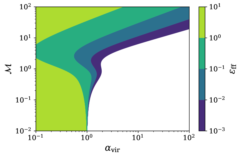
Figure 1: Star formation efficiency per freefall time as a function of the two parameters $\alpha_{\mathrm{vir}}$ and $\mathcal{M}$ in our modified multi-freefall model. For $\mathcal{M}\lesssim 1$, SF is only efficient if $\alpha_{\mathrm{vir}}\lesssim 1$ corresponding to the gravitational collapse of the whole computational cell. For higher values of $\mathcal{M}$, at fixed $\alpha_{\mathrm{vir}}$, the efficiency increases because of turbulent compression inside the cell at small, unresolved scales.

We now discuss some of the main caveats of the present approach. First, we have assumed a very simple spherical geometry for the collapsing transonic cores. This is not true in reality, where filamentary structures are very often seen in star forming regions (André et al., 2014). This effect could be parametrised through a multiplicative fudge factor in front of $\alpha_{\rm vir}$ in the collapse criteria.

Second, in the multi-freefall formulation, we have assumed that within each transonic core the efficiency of star formation is 100%, and no gas is left after stars are born. In our view, stellar feedback, as implemented in the next section, is responsible for terminating star formation. It is however possible to parametrise the efficiency of star formation per transonic cores using another multiplicative fudge factor in front of the integral in Equation 18.

Third, we have also considered collapsing fluid elements at the sonic scales, but larger, supersonic fluid elements could also collapse at a smaller density, further fragmenting into individual protostars. Such a model has been proposed for example by Hennebelle & Chabrier (2011) and Hopkins (2012).

Fourth, our lognormal model for the density fluctuations is only strictly speaking applicable to isothermal supersonic turbulence. At the relatively large scales considered here with $\Delta x\simeq$ 100 pc, the ISM is far from strictly isothermal. This can affect the density distribution in a non-trivial way (Robertson & Kravtsov, 2008). Having these caveats in mind, we nevertheless believe that any modification of the proposed model will not affect our results strongly, and certainly not at a qualitative level.

2.3 Subgrid model for stellar feedback

Stellar evolution is probably the most extreme subgrid aspect in galaxy formation. In principle, we need to follow the evolution of the internal structure of the stars, describe their evolution throughout their main sequence, until they die and explode, at least for the most massive ones. Although it is reasonable to assume that stellar interiors are fully decoupled from galactic scales, this is not true for the final explosive stages of stellar evolution.

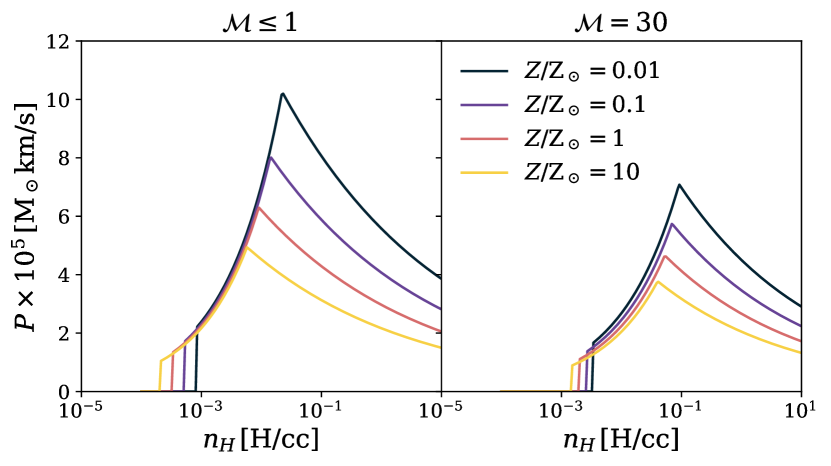
Figure 2: Injected scalar momentum for a single supernova explosion as a function of density. A resolution of $\Delta x_{\mathrm{min}}=150\mathrm{pc}$ is assumed here. Different colours show the injected momentum for various metallicities. For low density cells, we don’t inject momentum. For intermediate density cells, the cooling radius is resolved by at least one cell, but less than four cells. We compute the injected momentum using the Sedov solution. For high density cells, for which the cooling radius is not even resolved by one cell, we inject the terminal momentum. The left plot shows the injected momentum for a homogeneous medium, while the right plot corresponds to an inhomogeneous medium with $\mathcal{M}=30$ (from Martizzi et al., 2015).

Since our stellar particles have a typical mass of $\sim 10^{5}\mathrm{M}_{\odot}$, we have to account for individual supernovae using a subgrid model. For this, we assume that supernovae explosions within this single stellar population are uniformly distributed between $t_{\mathrm{start}}=3$ and $t_{\mathrm{end}}=20$ Myrs. At each simulation time step, we compute the supernova rate as

$$\dot{N}=\frac{\eta_{\mathrm{SN}}M_{\mathrm{ini}}}{M_{\mathrm{SN}}(t_{\mathrm{end}}-t_{\mathrm{start}})},$$ (22)

where $\eta_{\mathrm{SN}}=0.2$ is the mass fraction of the population that explodes in supernovae, $M_{\mathrm{ini}}$ is the initial mass of the stellar particle and $M_{\mathrm{SN}}=10\mathrm{M}_{\odot}$ is the typical mass of a single progenitor. Multiplying by the time step $\Delta t$, we obtain the expected (average) number of supernovae $\langle N\rangle=\dot{N}\Delta t$. The actual number of exploding supernova for a given stellar particle during the time step is drawn from a Poisson distribution (see Hopkins et al., 2018a, for a similar technique). This allows us to have supernovae explosions as discrete events realistically distributed in time, independent on the adopted mass resolution.

The other challenge of modelling supernovae explosions comes from the requirement of resolving the energy-conserving Sedov phase of the remnant. This phase is absolutely crucial as it is responsible for the momentum build-up that will later efficiently accelerate the surrounding gas. The scale that marks the transition from energy-conserving to momentum-conserving is the cooling radius $R_{\mathrm{cool}}$.

If the cooling radius is unresolved by the grid, which usually is the case for high gas densities, the thermal energy will be spuriously radiated away, without having the chance to create enough momentum. Therefore, to properly simulate the effects of supernova on the gas, we inject momentum additionally to the thermal injection if the cooling radius is not resolved. This technique, usually referred to as kinetic feedback or momentum feedback, has progressively emerged as one of the best subgrid models for supernovae explosions (Hopkins et al., 2014; Kimm & Cen, 2014; Kim et al., 2017; Agertz & Kravtsov, 2016; Rosdahl et al., 2017; Smith et al., 2018; Hopkins et al., 2018b).

On the other hand, if the cooling radius is resolved by the grid, which typically happens for low density gas, the supernova energy is directly injected in the form of thermal energy. The energy-conserving blast wave that will follow will then properly accelerate the gas around it and deliver the correct amount of momentum.

The terminal momentum of the momentum-conserving blast wave and the corresponding cooling radius can be computed analytically for homogeneous background densities and simple cooling functions. For more realistic cases, including explosions within a supersonic turbulent medium, we can use high-resolution simulations of individual explosions, such as in Martizzi et al. (2015). Using these numerical models, we use for the cooling radius

$$R_{\mathrm{cool}}=3.0\,\mathrm{pc}\left(\frac{Z}{Z_{\odot}}\right)^{-0.082}\left(\frac{n_{\mathrm{H}}}{100\,\mathrm{cm}^{-3}}\right)^{-0.42},$$ (23)

where $n_{\mathrm{H}}$ is the gas density of the cell where the star is exploding. If $R_{\mathrm{cool}}$ is unresolved by at least one grid cell, we inject for each individual supernova the terminal momentum $P_{\mathrm{SN}}$

$$P_{\mathrm{SN}}=1.42\times 10^{5}\mathrm{km\,s^{-1}M_{\odot}}\left(\frac{Z}{Z_{\odot}}\right)^{-0.137}\left(\frac{n_{\mathrm{H}}}{100\,\mathrm{cm}^{-3}}\right)^{-0.16}$$ (24)

Note that in the previous two equations, we use a metallicity floor at $0.01Z_{\odot}$ to model the effect of primordial cooling for a pristine gas. The total amount of injected scalar momentum from each star particle into its surrounding cell is

$$P=P_{\mathrm{SN}}N_{\mathrm{SN}}\min\left(1,\left(\frac{\Delta x_{\rm min}}{R_{\mathrm{cool}}}\right)^{3/2}\right)$$ (25)

where we use the Sedov solution when $\Delta x_{\rm min}<R_{\rm cool}<4\Delta x_{\rm min}$. Here $N_{\mathrm{SN}}$ is the number of supernovae for the current time step and for each star particle, while $\Delta x_{\rm min}$ is the minimum AMR cell size. Figure 2 shows the dependence of the injected momentum on the gas density for one supernova and for an adopted resolution of $\Delta x_{\mathrm{min}}=150\mathrm{pc}$. From Martizzi et al. (2015), we designed two models shown in Figure 2. The first one is valid for cells with a low Mach number, while the second one applies for high turbulent Mach number. In this paper, we use the low Mach number solution, but ideally, one should use the Mach number as an additional parameter. This model is unfortunately unavailable at the present time.

Once we know the injected scalar momentum per star particle, we need to deposit isotropically this momentum into the grid. For this, we use novel numerical techniques, inspired by the work of Agertz et al. (2013) and Hopkins et al. (2014).

First, we deposit the individual particle momentum onto the grid using the cloud-in-cell interpolation technique. We obtain the grid scalar momentum density $p=P/\Delta x^{3}$ and convert it into a momentum flux density using

$$Q=p\Delta x/\Delta t=P/\Delta x^{2}/\Delta t$$ (26)

Note that $Q$ is analogous to a pressure. This momentum flux is split equally among the 6 cell faces, defining a supernovae dynamical pressure noted $P_{\star}=Q/6$. This pressure only accounts for the momentum flux due to the supernovae explosions. It is directly added to the thermal pressure in the Riemann solver. This direct injection of momentum through the Riemann solver was first explored by Agertz et al. (2013), using non-thermal energy and pressure variables that are available in the RAMSES code. This method deposits the right amount of momentum to the gas, but also affects the thermal energy with undesirable effects (spurious heating or cooling of the gas).

We follow here a different approach by adding only this new pressure term in the momentum equation

$$\frac{\partial}{\partial t}\left(\rho v_{i}\right)+\frac{\partial}{\partial x_{j}}\left(\rho v_{i}v_{j}\right)+\frac{\partial}{\partial x_{i}}\left(P+P_{\star}\right)=-\rho\frac{\partial\phi}{\partial x_{i}}$$ (27)

and remove its corresponding $p{\rm d}V$ work from the energy equation, so that the internal energy equation remains unaffected by this momentum injection

$$\frac{\partial E}{\partial t}+\frac{\partial}{\partial x_{j}}\left(E+P+P_{\star}\right)v_{j}=P_{\star}\frac{\partial v_{j}}{\partial x_{j}}-\rho\frac{\partial\phi}{\partial x_{j}}v_{j}$$ (28)

This approach, a slight modification of the original method from Agertz et al. (2013), will deliver the proper momentum flux to neighbouring cells, together with consistent mass and energy fluxes. We also modify the time step stability condition, increasing the wave speed in the Courant condition to $|v|+c_{s}+p/\rho$, where $p$ is here the scalar momentum density defined above.

Our new method is more efficient than the traditional recipe for kinetic feedback in the RAMSES code, as implemented in Dubois & Teyssier (2008) and Kimm et al. (2015). These models inject the right solution at the relevant time of the deposition. In the limit of very poor resolution, they effectively inject the terminal momentum along with thermal energy. However, in these earlier attempts, the momentum is deposited on the grid using an explicit spherical velocity profile spread over a sphere of 4 cells in radius. This is usually done every coarse step and is quite costly. This is incompatible with our objective of resolving discrete supernovae with possibly a very high frequency of explosions.

On the other hand, depositing the momentum in only the 6 direct neighbours of the supernovae triggers spurious grid-aligned effects, especially if multiple supernovae explode in the same cell (Hopkins et al., 2018a). To avoid this, we choose the location of each individual explosion at random among the 8 cloud-in-cell neighbours from the star particle, suppressing visible grid alignment effects.

Although momentum feedback has proven quite successful in delivering the right amount of kinetic energy to the surrounding gas, a significant improvement over previous delayed cooling recipe, it still suffers from the caveat of not resolving properly the hot diffuse phase filling the cavity bounded by the momentum-conserving dense gas shell. This could affect the wind properties. Hu et al. (2014) have shown recently in the context of a dwarf galaxy that the main properties of the outflow are indeed captured by the momentum injection scheme, but properly describing the multiphase temperature structure of the wind requires to resolve the supernovae cooling radius.

Additionally, we model HII regions around young stars using a simple recipe for which we maintain the gas temperature (only in the cell where the star sits) at $10^{4}$ K for 20 Myr, until the last supernovae explodes. Thermal feedback from each supernova is modelled by injecting $E_{\mathrm{SN}}=10^{51}\mathrm{erg}$ in the parent cell. Furthermore, we assume that each supernova ejects $1\mathrm{M}_{\odot}$ of metal into the ISM.

3 Numerical experiments

We now report on the numerical experiment we have performed to test these new implementations of the key subgrid models for galaxy formation. For this, we model the cosmological evolution of a single dark matter halo, whose mass is comparable to the Milky Way mass, but whose accretion history is much more violent. In particular, we choose a halo with one major merger at relatively low redshift (expansion factor $a>0.5$). This will give us the opportunity to study how star formation and feedback behave in extreme cases. As it turned out, this particular halo features a strong starburst at $a=0.65$, followed by an extremely quiescent state, that we identify as a typical example of the population of early-type galaxies with long gas depletion time scales (Saintonge et al., 2011b). It is worth stressing that in our model we don’t use AGN feedback, so that any quenching mechanism here must be a consequence of our adopted stellar feedback and/or star formation models.

3.1 Simulation setup

We base our analysis on a cosmological zoom-in simulation that we performed with the AMR code RAMSES (Teyssier, 2002). We first ran a reference pure N-body simulation with $512^{3}$ particles in a periodic box of size 25 $h^{-1}$Mpc. First, we have selected all halos with masses in the range of $5\times 10^{11}\leq M_{\mathrm{vir}}/\mathrm{M}_{\odot}\leq 1.5\times 10^{12}$, where the virial mass is defined as the mass contained in a sphere of radius $R_{\mathrm{vir}}$ that encompasses an over-density of $200$ times the critical density. Secondly, we applied an isolation criterion at $z=0$ where halos are excluded if there is another halo within $5R_{\mathrm{vir}}$ with a mass of $10\%$ of the target halo. Finally, we looked at the mass-accretion histories of the available halos and selected one halo which experienced its last merger at $a=0.65$. This halo has a mass of $M_{\mathrm{vir}}=6.5\times 10^{11}$M_⊙ at $z=0$ and was used for our analysis.

We then generated new initial conditions around this halo with the MUSIC code (Hahn & Abel, 2011), with an initial hierarchy of concentric grids from $\ell_{\rm min}=7$, corresponding to a coarse grid resolution of $128^{3}$ covering the entire periodic box, to $\ell_{\rm max,ini}=10$, corresponding to an effective initial resolution of $1024^{3}$. This gives us a dark matter particle mass of $m_{\rm dm}=1.7\times 10^{6}$M_⊙ and a baryonic initial mass resolution of $m_{\rm dm}=2.6\times 10^{5}$M_⊙.

We then performed several simulations including gas and galaxy formation physics. The maximum resolution was set to $\ell_{\rm max}=18$ at $z=0$, while refinement levels were progressively released to enforce a constant physical resolution of $\Delta x_{\rm min}=100h^{-1}$pc. The adopted refinement criterion is the traditional quasi-Lagrangian approach, namely cells are individually refined when more than 8 dark matter particles are present or when the baryonic mass (gas and stars) exceed $8\times m_{\rm bar}$. Only the Lagrangian volume corresponding to twice the final virial radius of the halo was refined, the rest of the box being kept at a fixed, coarser resolution to provide the proper tidal field. Our zoom simulation corresponds to a halo slightly smaller than the Milky Way, but it features two successive major mergers, one at $a\simeq 0.35$ with a stellar mass ratio of 1:1 and a stellar mass of each galaxy of $M_{*}\simeq 1.5\times 10^{9}$M_⊙, and one later at $a\simeq 0.65$ with a stellar mas ratio of 1:1 too, and a larger galaxy stellar mass of $M_{*}\simeq 5\times 10^{9}$M_⊙. This scenario turned out to be an ideal one to study extreme regime of star formation and analyse the impact of our star formation and feedback recipe.

Gas cooling and heating is implemented using equilibrium chemistry for Hydrogen and Helium (Katz et al., 1996), together with the metallicity dependent cooling function for metals from Sutherland & Dopita (1993). Additionally, self-shielded UV-heating of the gas is taken into account, where the self-shielding density is assumed to be $n_{\mathrm{H}}=0.01\mathrm{H/cc}$ (Aubert & Teyssier, 2010). We adopt the model of Haardt & Madau (1996) for the UV background.

We ran three different simulations with different models for the galaxy formation physics.

1. The first simulation was run without feedback but using our new multi-freefall star formation model. It is labelled “no feedback” in the figures.

2. The second simulation was run with stellar feedback but adopting the old school constant efficiency model with $\epsilon_{\rm ff}=0.01$ and a star formation density threshold of $\rho_{*}=0.1$H/cc. It is labelled “constant efficiency” in the figures.

3. The third simulation was run with both our new recipe, namely stellar feedback and our varying $\epsilon_{\rm ff}$ model. It is labelled “varying efficiency” in the figures.

Note that we could have run the second simulation with a higher density threshold, to mimic a criterion $\alpha_{\rm vir}<1$ for some fixed temperature and Mach number. This would give results intermediate between our two cases. Note that if one adopts a high density threshold, $\rho_{*}=10$H/cc for example, it is impossible to form star in lower density gas, so that quenching occurs automatically in this case, in a rather ad-hoc way. Our multi-freefall approach, on the other hand, allows for star formation even in gas with $\alpha_{\rm vir}>1$ if the subgrid turbulence is strong enough.

We finally list our more technical RAMSES settings for these 3 simulations. We used the HLLC Riemann solver, modified to account for the supernovae dynamical pressure. The star particle was set equal to the baryonic mass resolution $m_{*}=m_{\rm bar}$. We adopted the MinMod slope limiter, an important choice to ensure the stability of the new feedback scheme. The adiabatic exponent of the gas was set to $\gamma=5/3$. We didn’t use any polytropic pressure floor, as our star formation model, by construction, very quickly removes gas for which the Jeans length is not resolved. The gas metallicity was initialised to $Z_{\rm ini}=10^{-3}Z_{\odot}$ to account for early population III stars enrichment.

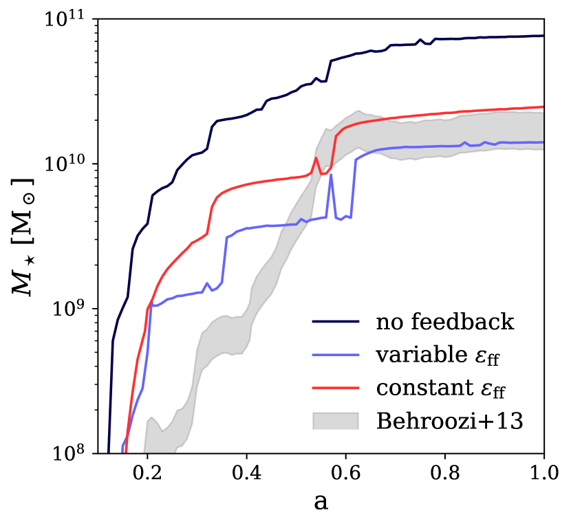
Figure 3: Evolution of the stellar mass as a function of the expansion factor in our 3 simulations. The shaded area represents the prediction from abundance matching according to Behroozi et al. (2013) using the virial mass of the halo at each time.

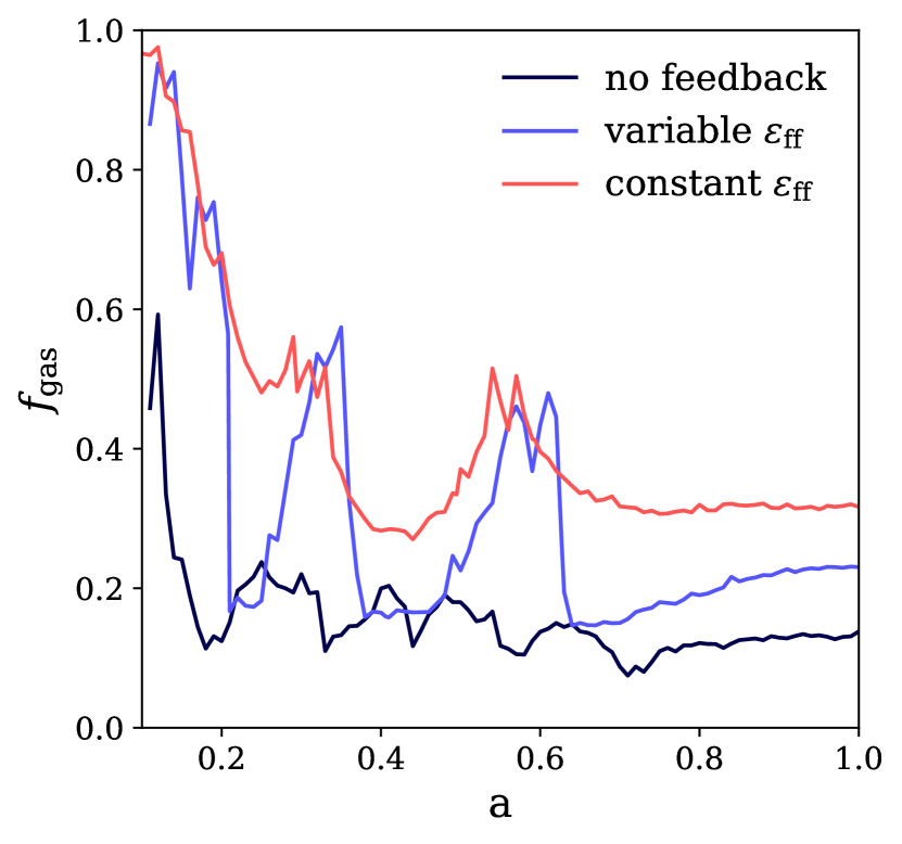
Figure 4: Evolution of the gas fraction inside $0.1R_{\mathrm{vir}}$ as a function of expansion factor for our 3 simulations. Sharp drops correspond to strong starburst-driven outflows with a large gas mass being removed.

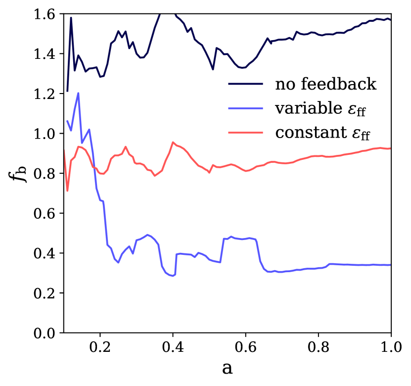
Figure 5: Evolution of the baryon fraction inside the virial radius as a function of expansion factor for our 3 simulations. In the no feedback run, the baryon fraction is 40% higher than the universal value, while in the varying efficiency model, 60% of the available baryons have been ejected outside the virial radius.

3.2 Effect of the feedback model

We plot in Figure 5 the evolution of the stellar mass of the central galaxy in our simulated galaxy for the 3 different subgrid models. The central galaxy is defined here as everything within $0.1\times R_{\rm vir}$ from the centre. As a validation test, we also show as a shaded area the expected stellar mass of the central galaxy from abundance matching (Behroozi et al., 2013), using the simulated halo mass as input at each epoch. The simulation without feedback completely overestimates the stellar mass (by a factor of 5), while our two models with feedback reproduce roughly the expected evolution. We see a clear trend for the constant efficiency model to produce almost twice as many stars than the multi-freefall model. The two major mergers in the mass accretion history of this particular halo can be seen as two jumps in the stellar mass of the central galaxy at $a\simeq 0.35$ and $a\simeq 0.65$.

In Figure 5, we show the evolution of the gas fraction within $0.1\times R_{\rm vir}$, defined by $f_{\mathrm{gas}}=M_{\mathrm{gas}}/(M_{\mathrm{gas}}+M_{\star})$. Ironically, the lowest gas fraction is obtained for the no feedback run, as most of the gas is consumed and turned into stars. The constant efficiency model, on the other hand, has the largest gas fraction, with $f_{\rm gas}\simeq 0.4$ at late time, while the varying efficiency model shows larger fluctuations, with peaks of gas fraction during star bursts, and a lower value of $f_{\rm gas}\simeq 0.2$ at late time, in better agreement with observation (see Discussion section). Our interpretation is that stellar feedback in the varying efficiency model is stronger, owing to the higher efficiency in the star bursts mode (see next Section). This is corroborated by Figure 5 that shows the baryon fraction with $R_{\rm vir}$. The no feedback case manages to accumulate more baryons in the virial radius than the universal fraction, while feedback maintains the baryon fraction below the universal value in all cases. The varying efficiency case, however, only retained 40% of the baryons in the halo, meaning that 60% of the baryons are lurking outside the virial radius, probably never coming back.

3.3 Effect of the star formation model

Although the stellar feedback subgrid model seems to play the main role in regulating the stellar mass of the galaxy, the star formation subgrid model seems to have a non-negligible impact on our results. The top panel of Figure 6 shows the star formation rate (SFR) as a function of the scale factor for our 2 models with feedback. It is defined as the instantaneous SFR within $0.1\times R_{\rm vir}$ at each time. We ignore the model without feedback in what follows because we believe it is not realistic. We clearly see the two major mergers as two strong starbursts with the SFR peaking at 10 $M_{\odot}~{}{\rm yr}^{-1}$. We used a bin size of $\Delta a=0.01$ corresponding roughly to 100 Myr at low redshifts.

In the varying efficiency case, the SFR during the starbursts is slightly larger than for the constant efficiency model. But this is after the starbursts that the difference between the 2 models is striking. The SFR for the varying efficiency model drops significantly down to 0.1 $M_{\odot}~{}{\rm yr}^{-1}$, while it remains quite high, around 1 $M_{\odot}~{}{\rm yr}^{-1}$ for the constant efficiency case.

This effect can be partly explained by the higher gas and baryon fraction in the constant efficiency case. Indeed, we see in the top panels of Figure 8 the morphological evolution of the corresponding central galaxy using true colour images with dust absorption that allows us to render both stars and gas. The constant efficiency case, owing to its higher gas and baryon fraction, leads to the formation of a large gaseous and star forming disk. This is a well-known outcome of gas-rich mergers (Hopkins et al., 2008; Daddi et al., 2010). The varying efficiency case, on the other hand, leads to the formation of a spheroidal galaxy with a tiny nuclear gas disk (see bottom panels of Fig. 8). In this case, the gas fraction is much lower, leading to the formation of dispersion dominated systems as explained by the gas-poor, dry merger scenario (Naab et al., 2007).

The origin of this difference can also be found in the star formation efficiency itself. In the lower panel of Figure 6, we plot the mean efficiency of the star forming gas within $0.1\times R_{\rm vir}$, defined as

$$\left<\epsilon_{\rm ff}\right>=\int\epsilon_{\rm ff}\frac{\rho}{t_{\rm ff}}{\rm d}V/\int\frac{\rho}{t_{\rm ff}}{\rm d}V$$ (29)

The constant efficiency with $\epsilon_{\rm ff}=0.01$ is also shown for comparison. We clearly see that during the starbursts the average efficiency peaks at up to 3%, while in the post-starburst quiescent phases, it drops down to 0.1%. The high efficiency we obtain during the mergers explains how the galaxy, although relatively gas poor compared to the other model, manages to have a SFR as high as 10 $M_{\odot}~{}{\rm yr}^{-1}$, like in the constant efficiency case. This helps maintaining the gas and baryon fractions low.

Note that this high efficiency is significantly higher than the critical value of 1% proposed by Semenov et al. (2018) that divides the feedback-dominated star formation regime from the efficiency-dominated star formation regime. Our constant efficiency model with $\epsilon_{\rm ff}=0.01$ sits just at the limit, so the resulting galaxy never reaches the feedback-dominated regime. Our varying efficiency model, on the other hand, clearly explores deep into these two regimes: 1- strong feedback-dominated starbursts, for which the exact value of $\epsilon_{\rm ff}$ probably plays a minor role, as long as it is larger than 1% and 2- long, extended, post-starbursts quiescent phases, for which the galaxy is quenched and the efficiency drops down to 0.1%.

In order to understand the origin of these wide variations in efficiency, we show in Figure 7 a mass-weighted histogram of the star forming gas within $0.1\times R_{\rm vir}$ in the $\alpha_{\rm vir}$-$\mathcal{M}$ plane. In the starburst case, at $a=0.65$, most of the star forming gas lies close to the 10% efficiency line. This is a combination of two factors: First, the merger event triggers the fast migration of gas to much higher density and smaller $\alpha_{\rm vir}$ (see e.g. Teyssier et al., 2010). The mean gas density during the starburst is roughly $n_{\rm H}\simeq 20$ H/cc. In the same time, the merger favours a higher gas turbulent velocity dispersion, with a mass-weighted average value as high as $\sigma_{\rm 1D}\simeq 70$ km/s. Both effects work in tandem to maintain the efficiency around 10% during the merger. This leads to extremely small depletion times, around 100 Myr, but the gas is also quickly collapsing and this high efficiency state can be maintained during the duration of the merger.

In the quiescent phase, we see in Figure 7 that most of the gas sits close to the 0.1% efficiency line. We are in the exact opposite situation than the starburst: residual gas accretion maintains a non-negligible, albeit lower, level of turbulence, around 20 km/s, while in the same time the mean gas density dropped to a rather low value with $n_{\rm H}\simeq 0.5$ H/cc. This leads to extremely long depletion times, around 10 Gyr. This residual star formation occurs mostly in a small nuclear disk a few kpc in size.

Milky Way-like galaxies correspond to the intermediate regime between the starburst and the quenched galaxy. We have explored this regime in a companion paper using a different halo (Kretschmer et al. in prep) and indeed, the mean efficiency settles naturally to 1% in the disk. Our varying efficiency model automatically adjusts its value to the conditions within the galaxy, each main galaxy type (starburst, disk, spheroid) giving rise to a different regime of star formation. This is due to a different structure of the ISM, with more or less gas being able to reach the limit of collapsing transonic cores.

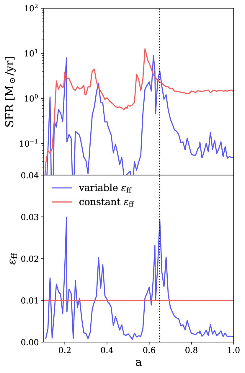
Figure 6: Top panel: The star formation history of the central galaxy as a function of the expansion factor for our two star formation models. Bottom panel: The average star formation efficiency per free fall time as a function of the expansion factor (see the exact definition in the text).

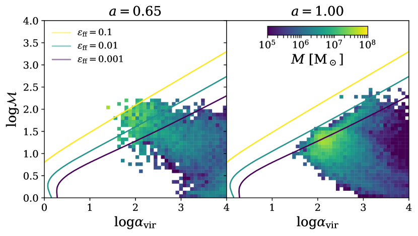
Figure 7: Mass-weighted histogram in the $\alpha_{\mathrm{vir}}$ and $\mathcal{M}$ phase-space at two different epochs. Left: the epoch of the starburst triggered by the last major merger. Right: the final epoch corresponding to the quenched, early-type galaxy. Coloured lines correspond to constant star formation efficiencies.

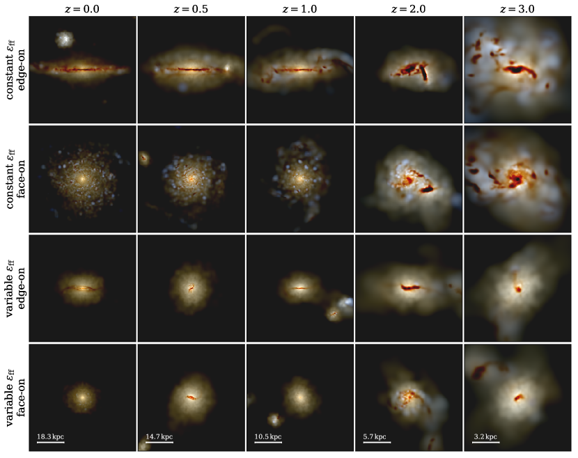
Figure 8: The morphological evolution of the corresponding central galaxy using true colour images with dust absorption allowing us to render both stars and gas. Each column from left to right shows the galaxy at a different redshift ($z=0.0,0.5,1.0,2.0,3.0$). Top 2 rows show the evolution of the galaxy with the constant $\epsilon_{\mathrm{ff}}$ star formation recipe, edge-on and face-on. The result is the formation of a large gaseous and star forming disk. Bottom 2 rows shows the evolution of the galaxy with the variable $\epsilon_{\mathrm{ff}}$ star formation recipe, edge-on and face-on. The resulting galaxy is a spheroidal galaxy with a tiny nuclear gas disk.

3.4 Effect of the subgrid turbulence model

The last important ingredient in our subgrid galaxy formation model is the SGS turbulence model. As explained in the previous section, we use a source term for the turbulent kinetic energy based on the local shear tensor and a sink term based on dissipation of kinetic energy over one turbulent crossing time. In order to test the robustness of our star formation model to the adopted model for turbulence, we decided to change the shear-based source term classically used in the SGS model by a supernova-based source term, in the spirit of the work of Semenov et al. (2016). Note that in the classical SGS model, supernovae explosions will also inject turbulence indirectly though momentum deposition followed by the corresponding shear-induced source term. We nevertheless turn the shear source term off and replace it by direct turbulent kinetic energy being deposited in the cell where the supernova explodes, assuming 10% of the energy in turbulent form.

The top panel of Figure 9 shows the evolution of the mass-weighted average turbulence resulting from these two models. The direct injection of turbulent energy from SN and the removal of the shear-based source term produces a level of turbulence roughly one order of magnitude smaller than the SGS model. Interestingly, this has a weak effect on the resulting star formation efficiency, as shown in the bottom panel of Figure 9. It is apparent that the difference between the two models is quite small, even though the actual level of turbulence is very different. This is because the varying efficiency model adapts to the local conditions in the galaxy and will transfer gas to smaller $\alpha_{\rm vir}$ (or higher density) compared to the SGS model, maintaining a similar star formation efficiency.

There is a small difference in scalefactor for the starburst at $a\simeq 0.65$ which originates from slightly different trajectories caused by numerical effects (Keller et al., 2019; Genel et al., 2019). Furthermore, the efficiencies for the SN induced turbulence model in the quiescent phases is larger compared to the efficiencies in the SGS run. Consider for example the left panel of Figure 7. In the SN turbulent case, many cells will have much smaller $\alpha_{\rm vir}$ and $\mathcal{M}$, bringing the individual gas cells into a regime where star formation is dominated by the collapse criterion through $\alpha_{\rm vir}$. Therefore, during a quite phase, in the SN injected turbulence case the efficiencies are larger because the small values for the turbulence will bring cells into a regime where star formation is controlled by the virial collapse.

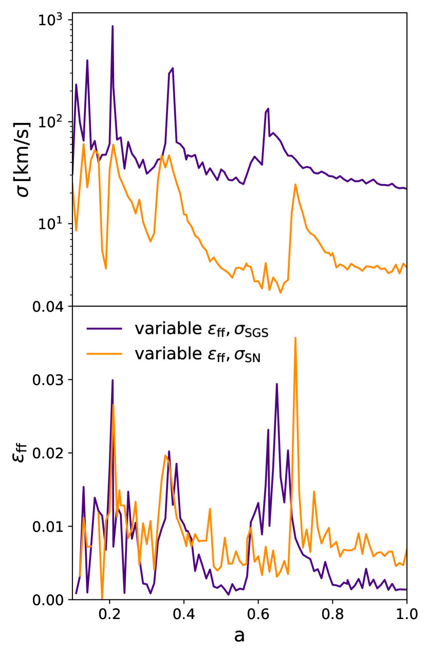
Figure 9: Top panel: Average turbulent velocity dispersion in the ISM as function of scale factor for two different source terms for turbulence. The SGS source term is based on the local shear and gives rise to larger velocity dispersions, compared to a source term based on direct kinetic energy injection by supernovae (SN). Bottom panel: The average star formation efficiency as a function of scale factor for the two different turbulent source terms.

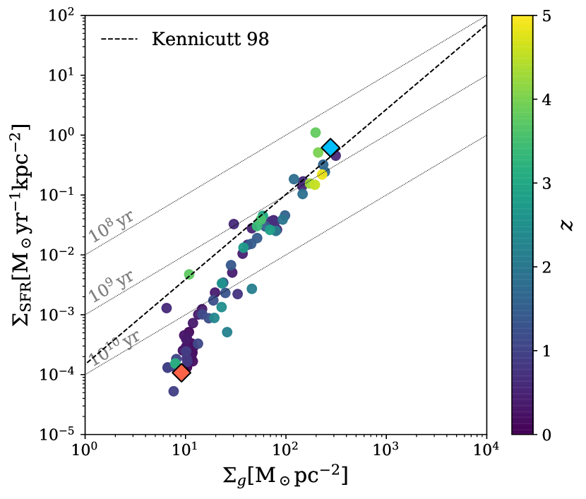
Figure 10: The unresolved KS diagram in the simulations. Each point is the average surface star formation rate and surface densities corresponding to a snapshot where the colour indicates the redshift. (See the text for the exact definition). The thin lines indicate constant depletion times of $10^{8},10^{9}$ and $10^{10}$ years. The dashed line is the empirical KS-law from (Kennicutt, 1998). The blue diamond symbol highlights the measured point during a starburst event at $a=0.65$ and the red highlights the obtained point for the quiescent phase $a=1.0$.

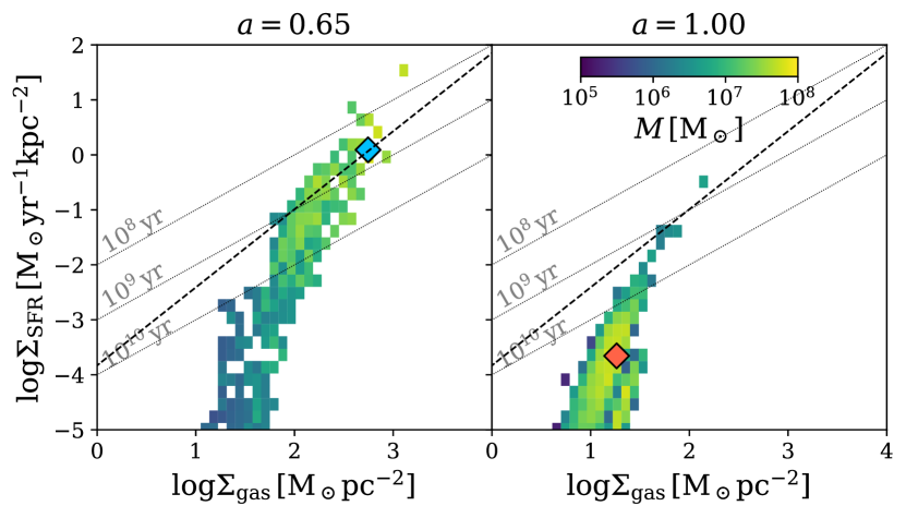
Figure 11: Mass-weighted distribution of the gas mass in a resolved KS diagram. Star formation and gas surface densities are computed in square patches of 200pc. The thin lines indicate constant depletion times of $10^{8},10^{9}$ and $10^{10}$ years. The dashed line is the empirical KS-law from (Kennicutt, 1998). Left is the distribution at $a=0.65$ during a starburst and right is the distribution at $a=1.0$ in a quiescent state. The diamond symbols are the averaged (global) values and the same as in Figure 10.

4 Discussion

In this paper, we have introduced a new set of subgrid models for star formation and feedback, uniquely combined in this new version of RAMSES. The feedback model, very similar qualitatively to earlier implementations of terminal momentum injection by supernovae, but quite different in the details, provides the first order mechanism for regulating the stellar and baryonic content in our simulated galaxies. The multi-freefall star formation model, based on a varying efficiency based on a subgrid turbulence model, allows us to form star without invoking arbitrary values for both the efficiency and the density threshold. We have shown that in a starburst regime, the efficiency can be significantly higher than 1%, at odd with traditional models of galaxy formation, while in a quenched regime, the efficiency can be as low as 0.1%, owing to the very different nature of the turbulent ISM in post-starburst, early-type galaxies.

Our star formation model, based on an SGS model for unresolved turbulence, and the subgrid model for supernovae momentum feedback are naturally designed in such a way that they are (relatively) resolution independent. When resolution is increased, the kinetic energy of turbulence will decrease, following the scaling for Burger’s (or Larson’s) turbulence. Ultimately, when the sonic length is resolved, the SGS turbulence will become subsonic and our star formation recipe with turn into a simple collapse criterion for thermally supported gas with 100% efficiency. At these scales, however, one usually adopts a sink particle formalism to describe star formation.

For supernovae feedback, increasing the resolution will allow us to resolve more the cooling radius, assuming the supernovae explode in a fixed density environment. This won’t be the case, unfortunately, as simulations with better and better resolution lead to denser and denser environments. In the limit of sub-parsec resolution, we know from dedicated ISM studies (Kimm & Cen, 2014; Walch et al., 2015; Iffrig & Hennebelle, 2017) that a crucial ingredient is the inclusion of walk-away and run-away massive stars. Overall, the galaxy formation simulations we present in this paper are far from resolving these scales, so that our subgrid models are crucial in providing a realistic treatment of these unresolved phenomena.

As explained in the previous section, our simulated halo allowed us to study two different regimes of star formation: a merger-induced starburst and a quenched early-type galaxy. The SFR in these two extreme cases are widely different, with 10 $M_{\odot}~{}{\rm yr}^{-1}$ for the starburst and 0.1 $M_{\odot}~{}{\rm yr}^{-1}$ for the early-type. These variations can be explained partly by the different gas fraction, but also by the different typical density and Mach number in these galaxies. We now compare the properties of our simulated galaxy to observed ones using the global KS relation in Figure 10. For this, we compute the total star formation rate in the galaxy by integrating the star formation rate in each gas cell within $0.1\times R_{\rm vir}$ and the total gas mass within the same region. We then use the half-mass radius of the gas $r_{h}$ to compute the global surface densities of both star formation and gas as (Freundlich et al., 2019)

$$\dot{\Sigma}_{*}=0.5\frac{\dot{M}_{*}}{\pi r^{2}_{h}}~{}~{}~{}{\rm and}~{}~{}~{}\Sigma_{\rm gas}=0.5\frac{M_{\rm gas}}{\pi r^{2}_{h}}.$$ (30)

In Figure 10, each symbol corresponds to the location of the galaxy in the global KS diagram at a different epoch. We also indicate 3 lines corresponding to a constant depletion time of 100 Myr, 1 Gyr and 10 Gyr. Although high redshift conditions lead in general to small depletion times, the galaxy is moving quite widely along the KS relation (Tacchella et al., 2016, 2018). The two diamond symbols show the most extreme conditions we have obtained, with the starburst at the rightmost tip of the KS relation, and the quenched early-type at the leftmost end.

To understand better the origin of these two extreme cases, we show in Figure 11 the distribution of the gas mass in a resolved KS diagram. For this, we compute the star formation and gas surface densities using square patches of 200 pc size and compare it to the observed KS relation as well as constant depletion time models. In each case (starburst and early-type) we also show as a single diamond symbol the global values. We clearly see that the gas and star formation surface densities is the starburst case are both very large, with very small depletion times, around 1 Gyr in average but as small as 100 Myr in some regions. The early-type galaxy at the final epoch, on the other hand, has an average depletion time around 20 Gyr, with some regions reaching barely 1 Gyr.

In order to compare to molecular observations, we use the model of Vallini et al. (2018) to compute the molecular $\rm H_{2}$ mass within each cell, assuming for the interstellar radiation field a global uniform value given by $G=G_{0}(\mathrm{SFR/M}_{\odot}{\rm yr}^{-1})$ at each epoch. For the merger-induced starburst at $a\simeq 0.65$, we find $M_{\rm gas}\simeq 2\times 10^{9}~{}M_{\odot}$ and $M_{\mathrm{H}_{2}}\simeq 9\times 10^{8}~{}\rm M_{\odot}$, while for the early-type quenched galaxy at $a=1$ we have $M_{\rm gas}\simeq 4\times 10^{9}~{}\rm M_{\odot}$ and $M_{\rm H_{2}}\simeq 8\times 10^{8}~{}\rm M_{\odot}$. Note that our model for $\rm H_{2}$ formation is based on exactly the same turbulence-based subgrid model for star formation, so that there is a built-in correlation between star formation and molecular gas formation, but no direct causal relation.

In the early-type case, the long depletion time coincides with a low $H_{2}$ fraction, so that the molecular gas depletion time becomes shorter by a factor of $\sim 5$, around 20 Gyr. This is in perfect agreement with the COLD GASS sample observed at IRAM (Saintonge et al., 2011a, b), with our early-type case corresponding to a low specific star formation rate $\mathrm{sSFR}\simeq 10^{-12}~{}{\rm yr}^{-1}$ and long molecular depletion times $t_{\rm dep}(\rm H_{2})\simeq 20$ Gyr, and our starburst case corresponding to LIRGs or ULIRGs (see Fig. 9 in Saintonge et al., 2011b).

Interestingly, post-starburst galaxies show many similarities with our quenched mode of star formation. In several recent papers, galaxies showing signs of recent starburst activity are completely quenched, although they contain enough gas to form stars at a rate much higher than observed (van de Voort et al., 2018; Ellison et al., 2018; Smercina et al., 2018). Residual turbulence in the ISM or high levels of radiation were proposed as possible explanations to quench star formation in such systems. These systems are probably ideal examples of galaxies with a very peculiar ISM structure, leading to an exceptionally low star formation efficiency.

At late times the baryon fraction in the halo stays constant. At the same time the gas fraction in the disk increases by $\sim 10\%$ due to gas cooling from the halo onto the disk. The star formation rate however does not increase with the gas fraction but rather decreases. This is because the efficiency depends on the shear-induced turbulence in a non-linear way. Namely the level of turbulence in the disk from accretion or shear will prevent star formation. In contrast, the star formation rate given by the constant efficiency model does increase with the gas fraction of that run.

Another interesting class of objects are circumnuclear disks at the centre of early-type galaxies. Our simulation with varying efficiency shows at the final epoch such a nuclear disk (see Fig. 8). Nuclear disks in early-type galaxies are compact, relatively dense in their centre with $\Sigma_{\rm gas}\simeq 100~{}\rm M_{\odot}~{}{\rm pc}^{-2}$ but very inefficient in forming stars (Davis et al., 2014), when compared to normal galaxies with the same gas surface densities. The strong shear observed in these systems was proposed as an explanation for their surprisingly low star formation efficiency. One particularly striking example is NGC 4429 from the same ATLAS3D sample: In a recent attempt to model it, Naab and co-workers (private communication) had to use a constant efficiency of $\epsilon_{\rm ff}\simeq 0.2\%$ to reproduce various properties such as gas content and star formation rate. This is very close to the efficiency we obtained using the varying efficiency model in our final early-type galaxy.

5 Summary and Conclusion

In this paper, we have introduced a new implementation of recently proposed subgrid models for star formation and feedback in the RAMSES code. The stellar feedback model is based on individual, discrete Type II supernova events. If the radius marking the transition from the energy-conserving phase to the momentum-conserving phase is unresolved by our computational cell, we inject directly momentum in the neighbourhood of the exploding star. This is done by modifying the Riemann solver in our Godunov scheme, allowing us to deliver the right amount of momentum, together with consistent mass and energy fluxes.

The multi-freefall star formation model is based on a subgrid turbulence model and provides a varying star formation efficiency that depends on the local conditions in each computational cell, through the cell’s virial parameter and its turbulent Mach number. The star formation efficiency can be very large for large density fluctuations caused by supersonic turbulence, as expected, for example, during a merger. On the other hand, the star formation efficiency can be very low for subsonic and marginally stable disks, as expected during more quiescent phases or in early-type galaxies. This new versatile model allows us to form star without invoking arbitrary values for both the efficiency and the density threshold.

We apply this new implementation of subgrid galaxy formation physics to a prototype cosmological simulation of a massive halo that features a major merger, and study specifically the interesting case of the formation of an early-type galaxy. We find that the feedback model provides the first order mechanism for regulating the stellar and baryonic content in our simulated galaxies. Together with the multi-freefall star formation model, feedback is strong during starbursts. At redshift zero, only 40% of baryons are retained in the halo and the gas fraction is $\sim 20\%$. The resulting stellar masses are in good agreement with those expected from abundance matching results.

In a starburst regime, the efficiencies can be significantly higher than 1%, at odd with traditional models of galaxy formation, while in a quenched regime, the efficiencies can be as low as 0.1%, owing to the very different nature of the turbulent ISM in post-starburst, early-type galaxies. Indeed, the merger driven event pushes gas to large densities and large turbulent velocity dispersions, which causes larger $\mathcal{M}$ and small $\alpha_{\mathrm{vir}}$. As a result, efficiencies can reach locally $10\%$ and the $\mathrm{sSFR}$ is large. The small value for the molecular gas depletion time during the starburst is in perfect agreement with observations. Additionally, at late times, when the galaxy is quiescent, the $\mathrm{sSFR}$ is small and the molecular gas depletion time is long, also in perfect agreement with observations.

In summary, at high redshifts, very efficient star formation together with strong feedback regulates the baryonic content. At low redshift, local star formation becomes very inefficient explaining the properties of quenched galaxies.

References

- Agertz & Kravtsov (2016) Agertz O., Kravtsov A. V., 2016, ApJ, 824, 79
- Agertz et al. (2011) Agertz O., Teyssier R., Moore B., 2011, MNRAS, 410, 1391
- Agertz et al. (2013) Agertz O., Kravtsov A. V., Leitner S. N., Gnedin N. Y., 2013, ApJ, 770, 25
- Agertz et al. (2020) Agertz O., et al., 2020, MNRAS, 491, 1656
- André et al. (2014) André P., Di Francesco J., Ward-Thompson D., Inutsuka S. I., Pudritz R. E., Pineda J. E., 2014, in Beuther H., Klessen R. S., Dullemond C. P., Henning T., eds, Protostars and Planets VI. p. 27 (arXiv:1312.6232), doi:10.2458/azu_uapress_9780816531240-ch002
- Aubert & Teyssier (2010) Aubert D., Teyssier R., 2010, ApJ, 724, 244
- Balogh et al. (2001) Balogh M. L., Pearce F. R., Bower R. G., Kay S. T., 2001, MNRAS, 326, 1228
- Baugh (2006) Baugh C. M., 2006, Reports on Progress in Physics, 69, 3101
- Behroozi et al. (2013) Behroozi P. S., Wechsler R. H., Conroy C., 2013, ApJ, 770, 57
- Benson et al. (2000) Benson A. J., Cole S., Frenk C. S., Baugh C. M., Lacey C. G., 2000, MNRAS, 311, 793
- Borgani & Kravtsov (2011) Borgani S., Kravtsov A., 2011, Advanced Science Letters, 4, 204
- Capelo et al. (2018) Capelo P. R., Bovino S., Lupi A., Schleicher D. R. G., Grassi T., 2018, MNRAS, 475, 3283
- Cen & Ostriker (1992) Cen R., Ostriker J. P., 1992, ApJ, 399, 331
- Cole et al. (2001) Cole S., et al., 2001, MNRAS, 326, 255
- Daddi et al. (2010) Daddi E., et al., 2010, ApJ, 713, 686
- Davis et al. (2014) Davis T. A., et al., 2014, MNRAS, 444, 3427
- Dekel & Silk (1986) Dekel A., Silk J., 1986, ApJ, 303, 39
- Dekel et al. (2009) Dekel A., et al., 2009, Nature, 457, 451
- Dubois & Teyssier (2008) Dubois Y., Teyssier R., 2008, A&A, 477, 79
- Ellison et al. (2018) Ellison S. L., Catinella B., Cortese L., 2018, MNRAS, 478, 3447
- Federrath & Klessen (2012) Federrath C., Klessen R. S., 2012, ApJ, 761, 156
- Feldmann & Gnedin (2011) Feldmann R., Gnedin N. Y., 2011, ApJ, 727, L12
- Feldmann et al. (2010) Feldmann R., Carollo C. M., Mayer L., Renzini A., Lake G., Quinn T., Stinson G. S., Yepes G., 2010, ApJ, 709, 218
- Fielding et al. (2017) Fielding D., Quataert E., Martizzi D., Faucher-Giguère C.-A., 2017, MNRAS, 470, L39
- Freundlich et al. (2019) Freundlich J., et al., 2019, A&A, 622, A105
- Fukugita et al. (1998) Fukugita M., Hogan C. J., Peebles P. J. E., 1998, ApJ, 503, 518
- Genel et al. (2019) Genel S., et al., 2019, ApJ, 871, 21
- Guo et al. (2010) Guo Q., White S., Li C., Boylan-Kolchin M., 2010, MNRAS, 404, 1111
- Haardt & Madau (1996) Haardt F., Madau P., 1996, ApJ, 461, 20
- Hahn & Abel (2011) Hahn O., Abel T., 2011, MNRAS, 415, 2101
- Hennebelle & Chabrier (2011) Hennebelle P., Chabrier G., 2011, ApJ, 743, L29
- Hopkins (2012) Hopkins P. F., 2012, MNRAS, 423, 2037
- Hopkins et al. (2008) Hopkins P. F., Hernquist L., Cox T. J., Kereš D., 2008, ApJS, 175, 356
- Hopkins et al. (2011) Hopkins P. F., Quataert E., Murray N., 2011, MNRAS, 417, 950
- Hopkins et al. (2014) Hopkins P. F., Kereš D., Oñorbe J., Faucher-Giguère C.-A., Quataert E., Murray N., Bullock J. S., 2014, MNRAS, 445, 581
- Hopkins et al. (2018a) Hopkins P. F., et al., 2018a, MNRAS, 477, 1578
- Hopkins et al. (2018b) Hopkins P. F., et al., 2018b, MNRAS, 480, 800
- Hu (2019) Hu C.-Y., 2019, MNRAS, 483, 3363
- Hu et al. (2014) Hu C.-Y., Naab T., Walch S., Moster B. P., Oser L., 2014, MNRAS, 443, 1173
- Iffrig & Hennebelle (2017) Iffrig O., Hennebelle P., 2017, A&A, 604, A70
- Katz et al. (1992) Katz N., Hernquist L., Weinberg D. H., 1992, ApJ, 399, L109
- Katz et al. (1996) Katz N., Weinberg D. H., Hernquist L., 1996, ApJS, 105, 19
- Keller et al. (2019) Keller B. W., Wadsley J. W., Wang L., Kruijssen J. M. D., 2019, MNRAS, 482, 2244
- Kennicutt (1998) Kennicutt Robert C. J., 1998, ApJ, 498, 541
- Kennicutt et al. (2007) Kennicutt Robert C. J., et al., 2007, ApJ, 671, 333
- Kereš et al. (2005) Kereš D., Katz N., Weinberg D. H., Davé R., 2005, MNRAS, 363, 2
- Kim et al. (2017) Kim C.-G., Ostriker E. C., Raileanu R., 2017, ApJ, 834, 25
- Kimm & Cen (2014) Kimm T., Cen R., 2014, ApJ, 788, 121
- Kimm et al. (2015) Kimm T., Cen R., Devriendt J., Dubois Y., Slyz A., 2015, MNRAS, 451, 2900
- Krumholz & McKee (2005) Krumholz M. R., McKee C. F., 2005, ApJ, 630, 250
- Krumholz & Tan (2007) Krumholz M. R., Tan J. C., 2007, ApJ, 654, 304
- Lada et al. (2010) Lada C. J., Lombardi M., Alves J. F., 2010, ApJ, 724, 687
- Lupi et al. (2018) Lupi A., Bovino S., Capelo P. R., Volonteri M., Silk J., 2018, MNRAS, 474, 2884
- Mac Low & Klessen (2004) Mac Low M.-M., Klessen R. S., 2004, Reviews of Modern Physics, 76, 125
- Macciò et al. (2017) Macciò A. V., Frings J., Buck T., Penzo C., Dutton A. A., Blank M., Obreja A., 2017, MNRAS, 472, 2356
- Martizzi et al. (2015) Martizzi D., Faucher-Giguère C.-A., Quataert E., 2015, MNRAS, 450, 504
- McKee & Ostriker (2007) McKee C. F., Ostriker E. C., 2007, ARA&A, 45, 565
- Moster et al. (2010) Moster B. P., Somerville R. S., Maulbetsch C., van den Bosch F. C., Macciò A. V., Naab T., Oser L., 2010, ApJ, 710, 903
- Murray (2011) Murray N., 2011, ApJ, 729, 133
- Naab & Ostriker (2017) Naab T., Ostriker J. P., 2017, ARA&A, 55, 59
- Naab et al. (2007) Naab T., Johansson P. H., Ostriker J. P., Efstathiou G., 2007, ApJ, 658, 710
- Naab et al. (2014) Naab T., et al., 2014, MNRAS, 444, 3357
- Ocvirk et al. (2008) Ocvirk P., Pichon C., Teyssier R., 2008, MNRAS, 390, 1326
- Oppenheimer & Davé (2006) Oppenheimer B. D., Davé R., 2006, MNRAS, 373, 1265
- Oppenheimer et al. (2010) Oppenheimer B. D., Davé R., Kereš D., Fardal M., Katz N., Kollmeier J. A., Weinberg D. H., 2010, MNRAS, 406, 2325
- Ostriker et al. (2010) Ostriker E. C., McKee C. F., Leroy A. K., 2010, ApJ, 721, 975
- Padoan & Nordlund (2011) Padoan P., Nordlund Å., 2011, ApJ, 730, 40
- Padoan et al. (2012) Padoan P., Haugbølle T., Nordlund Å., 2012, ApJ, 759, L27
- Perret et al. (2015) Perret V., Teyssier R., Devriendt J., Rosdahl J., Slyz A., 2015, in IAU General Assembly. p. 2257403
- Persic & Salucci (1992) Persic M., Salucci P., 1992, MNRAS, 258, 14P
- Pontzen et al. (2013) Pontzen A., Roškar R., Stinson G., Woods R., 2013, pynbody: N-Body/SPH analysis for python (ascl:1305.002)
- Rasera & Teyssier (2006) Rasera Y., Teyssier R., 2006, A&A, 445, 1
- Renaud et al. (2015) Renaud F., Bournaud F., Duc P.-A., 2015, MNRAS, 446, 2038
- Robertson & Kravtsov (2008) Robertson B. E., Kravtsov A. V., 2008, ApJ, 680, 1083
- Rosdahl et al. (2017) Rosdahl J., Schaye J., Dubois Y., Kimm T., Teyssier R., 2017, MNRAS, 466, 11
- Roškar et al. (2014) Roškar R., Teyssier R., Agertz O., Wetzstein M., Moore B., 2014, MNRAS, 444, 2837
- Saintonge et al. (2011a) Saintonge A., et al., 2011a, MNRAS, 415, 32
- Saintonge et al. (2011b) Saintonge A., et al., 2011b, MNRAS, 415, 61
- Schmidt (2014) Schmidt W., 2014, Numerical Modelling of Astrophysical Turbulence
- Schmidt & Federrath (2011) Schmidt W., Federrath C., 2011, A&A, 528, A106
- Schmidt et al. (2006a) Schmidt W., Niemeyer J. C., Hillebrandt W., 2006a, A&A, 450, 265
- Schmidt et al. (2006b) Schmidt W., Niemeyer J. C., Hillebrandt W., Röpke F. K., 2006b, A&A, 450, 283
- Semenov et al. (2016) Semenov V. A., Kravtsov A. V., Gnedin N. Y., 2016, ApJ, 826, 200
- Semenov et al. (2018) Semenov V. A., Kravtsov A. V., Gnedin N. Y., 2018, ApJ, 861, 4
- Shapley et al. (2003) Shapley A. E., Steidel C. C., Pettini M., Adelberger K. L., 2003, ApJ, 588, 65
- Silk & Rees (1998) Silk J., Rees M. J., 1998, A&A, 331, L1
- Smagorinsky (1963) Smagorinsky J., 1963, Monthly Weather Review, 91, 99
- Smercina et al. (2018) Smercina A., et al., 2018, ApJ, 855, 51
- Smith et al. (2018) Smith M. C., Sijacki D., Shen S., 2018, MNRAS, 478, 302
- Springel et al. (2005) Springel V., Di Matteo T., Hernquist L., 2005, MNRAS, 361, 776
- Steidel et al. (2010) Steidel C. C., Erb D. K., Shapley A. E., Pettini M., Reddy N., Bogosavljević M., Rudie G. C., Rakic O., 2010, ApJ, 717, 289
- Stinson et al. (2006) Stinson G., Seth A., Katz N., Wadsley J., Governato F., Quinn T., 2006, MNRAS, 373, 1074
- Sutherland & Dopita (1993) Sutherland R. S., Dopita M. A., 1993, ApJS, 88, 253
- Tacchella et al. (2016) Tacchella S., Dekel A., Carollo C. M., Ceverino D., DeGraf C., Lapiner S., Mandelker N., Primack Joel R., 2016, MNRAS, 457, 2790
- Tacchella et al. (2018) Tacchella S., et al., 2018, ApJ, 859, 56
- Teyssier (2002) Teyssier R., 2002, A&A, 385, 337
- Teyssier et al. (2010) Teyssier R., Chapon D., Bournaud F., 2010, ApJ, 720, L149
- Teyssier et al. (2011) Teyssier R., Moore B., Martizzi D., Dubois Y., Mayer L., 2011, MNRAS, 414, 195
- Teyssier et al. (2013) Teyssier R., Pontzen A., Dubois Y., Read J. I., 2013, MNRAS, 429, 3068
- Trebitsch et al. (2017) Trebitsch M., Blaizot J., Rosdahl J., Devriendt J., Slyz A., 2017, MNRAS, 470, 224
- Trebitsch et al. (2018) Trebitsch M., Volonteri M., Dubois Y., Madau P., 2018, MNRAS, 478, 5607
- Vallini et al. (2018) Vallini L., Pallottini A., Ferrara A., Gallerani S., Sobacchi E., Behrens C., 2018, MNRAS, 473, 271
- Walch et al. (2015) Walch S., et al., 2015, MNRAS, 454, 238
- Wheeler et al. (2019) Wheeler C., et al., 2019, MNRAS, 490, 4447
- van de Voort et al. (2018) van de Voort F., et al., 2018, MNRAS, 476, 122