Coherence assisted non-Gaussian measurement device independent quantum key distribution

Abstract

Non-Gaussian operations on two mode squeezed vacuum states (TMSV) in continuous variable measurement device independent quantum key distribution (CV-MDI-QKD) protocols have been shown to effectively increase the total transmission distances drastically. In this paper we show that photon subtraction on a two mode squeezed coherent (PSTMSC) state can further improve the transmission distances remarkably. To that end we also provide a generalized covariance matrix corresponding to PSTMSC, which has not been attempted before. We show that coherence, defined as the amount of displacement of vacuum state, along with non-Gaussianity can help improve the performance of prevalent CV-MDI-QKD protocols. Furthermore, since we use realistic parameters, our technique is experimentally feasible and can be readily implemented.

I Introduction

Quantum key distribution(QKD) protocols Gisin et al. (2002); Pirandola et al. (2019) provide a way to carry out unconditionally secure communication which is not possible in the classical world. Prevalent QKD schemes can be divided into two main categories: discrete variable QKD (DV-QKD) Ekert (1991); Bennett and Brassard (1984) and continuous variable QKD (CV-QKD) Cerf et al. (2001); Grosshans and Grangier (2002); Hillery (2000); Ralph (1999). While the DV-QKD protocols were developed first, CV-QKD are more readily compatible with current communication technologies and do not require costly single photon sources or detectors. Protocols based on CV systems have also been shown to be unconditionally secure against collective attacks Leverrier et al. (2013); Leverrier (2015, 2017); Renner and Cirac (2009); Shor and Preskill (2000) in the finite key size and asymptotic regime and have been experimentally implemented Bennett et al. (1992); Grosshans et al. (2003); Wang et al. (2013).

One of the main drawbacks of both the schemes is that in practice the devices being used may themselves be imperfect which may lead to serious potential security vulnerabilities not modelled theoretically. In order to identify all such security loopholes or side-channels, it is necessary to fully characterize the devices being used, which in itself is an arduous task. However, by clever use of entanglement swapping, it is possible to bypass this strict characterization of devices which led to the development of discrete variable measurement device independent quantum key distribution(DV-MDI-QKD) scheme Braunstein and Pirandola (2012); Lo et al. (2012). In this scheme a third untrusted party performs Bell state measurements, whose results are publicly communicated and used in the process of sharing the secure key. These protocols have been extensively analyzed both theoretically Curty et al. (2014); Ottaviani et al. (2015); Wang (2013) as well as experimentally Rubenok et al. (2013); Ferreira da Silva et al. (2013); Liu et al. (2013). Quite soon CV versions of MDI-QKD were proposed based on similar ideas of entanglement swapping Pirandola et al. (2015); Li et al. (2014); Ma et al. (2014). These protocols have also been studied theoretically Papanastasiou et al. (2017); Lupo et al. (2018); Wang et al. (2018) and realized experimentally Pirandola et al. (2015). However, the maximal transmission distances were found to be unsatisfactory as compared to DV-MDI-QKD. Several investigations have found that non-Gaussian operations, like photon addition and subtraction can be used to increase the entanglement content of the underlying two mode squeezed states Ourjoumtsev et al. (2007); Lee et al. (2011); Zhang and van Loock (2010); Bose and Kumar (2017); Dell’Anno et al. (2007); Hu et al. (2017); Navarrete-Benlloch et al. (2012); Yang and Li (2009). It is therefore natural to assume that they can be helpful in improving the maximum transmission distances Ma et al. (2018); Zhao et al. (2018) of CV-MDI-QKD. Specifically, photon subtraction on two mode squeezed vacuum state (PSTMSV) has been shown to increase transmission distances Ma et al. (2018) as compared to two mode squeezed vacuum (TMSV) or two mode squeezed coherent (TMSC) state. There have also been indications that coherence might be useful in improving the efficiency of CV-MDI-QKD protocols, while most of the analysis has been restricted to non-Gaussian operations on TMSV states. However, it should also be noted that application of non-Gaussian operations on the TMSC state is theoretically quite difficult and a tedious task, which to the best of our knowledge has not been attempted in full generality before.

In this paper we show that non-Gaussianity coupled with small displacements (termed as coherence) of the vacuum state can significantly increase the transmission distances, with a slight decrease in the maximum achievable secure key rate for the CV-MDI-QKD schemes. We show that transmission distances can be drastically improved upto $60-70$ Kms using the same. Specifically, we apply photon subtraction on the TMSC state and use it in a general CV-MDI-QKD scheme. We then show that several previous CV-MDI-QKD protocols based on either Gaussian or non-Gaussian resources can be recovered as special cases of our protocol. We provide the analysis of secure key rate and explicitly identify coherence as a new and better resource along with non-Gaussianity for improving transmission distances of prevalent CV-MDI-QKD for experimentally realizable parameter range. In this process we explicitly calculate the covariance matrix corresponding to $k$-PSTMSC state, which in itself is quite interesting and can find application in various other research problems in the field of CV quantum information processing.

The paper is organized as follows. In Sec. II we first review the technique of CV-MDI-QKD and provide a modified version tailored for PSTMSC state which is used throughout the paper. In Sec. IV we provide numerical simulations of the performance of PSTMSC state in CV-MDI-QKD, while in Sec. V we draw conclusions from our results and look at future aspects.

II CV-MDI QKD on PSTMSC

In this section we first review the basic concepts of CV-MDI-QKD with a focus on its entanglement based (EB) variant and then move on to explain our protocol based on photon subtraction on a two mode squeezed coherent state (PSTMSC).

II.1 CV-MDI QKD

In the original entanglement based version of CV-MDI-QKD, two parties Alice and Bob each prepare a TMSV state with quadrature variances $V_{A}$ and $V_{B}$. We assume that $V_{A}=V_{B}$ throughout the paper.

The pairs of modes are labelled as $A_{1}$, $A_{2}$ and $B_{1}$, $B_{2}$ respectively for Alice and Bob. Alice and Bob both transmit one of their modes, $A_{2}$ and $B_{2}$, to a third untrusted party Charlie via quantum channels with lengths $L_{AC}$ and $L_{BC}$ respectively, while retaining the modes $A_{1}$ and $B_{1}$ with themselves. The total transmission length is $L=L_{AC}+L_{BC}$. Charlie interferes the two modes with the help of a beam splitter (BS) which has two output modes $C$ and $D$. He then performs a homodyne measurement of $x$ quadrature on mode $C$ with outcome $X_{C}$ and $p$ quadrature on mode $D$ with outcome $P_{D}$ and publicly announces the obtained outcomes $\{X_{C},P_{D}\}$.

With the publicly available knowledge of $\{X_{C},P_{D}\}$, Bob transforms his retained mode $B_{1}$ to $B^{\prime}_{1}$ by a displacement operation $D(\beta)$, where $\beta=g(X_{C}+iP_{D})$ and $g$ is the gain factor. Consequently, the modes $A_{1}$ and $B^{\prime}_{1}$ become entangled. Later, Alice and Bob both perform a heterodyne measurement on the modes $A_{1}$ and $B^{\prime}_{1}$ to obtain the outcomes $\{X_{A},P_{A}\}$ and $\{X_{B},P_{B}\}$ respectively, which end up being correlated. Finally both the parties perform information reconciliation and privacy amplification to obtain the secret key.

II.2 Photon subtraction on two mode squeezed coherent state

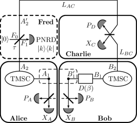
Figure 1: Scheme of CV-MDI-QKD using PSTMSC state. The scheme represents various operations performed by several parties of which Fred and Charlie are untrusted. After displacement of mode $B_{1}$ by Bob based on results announced by Charlie, the modes $A_{1}$ and $B^{\prime}_{1}$ become correlated.

In this paper we perform EB CV-MDI-QKD by implementing photon subtraction on a TMSC state. The additional parameter in our protocol is the fact that we are starting with coherent state with a finite displacement before squeezing it.

Furthermore, we assume that Bob performs reverse reconciliation (RR), which means that outcomes obtained by Bob are taken as reference for Alice to reconcile. Here, we describe the basic schematic of the protocol is given in Fig. 1 while relevant calculations are shown in Appendix with explicit use of phase-space methods, in particular by using Wigner function description. We describe the entire protocol through the following steps.

Step 1. Alice prepares a TMSC state $|\psi\rangle_{A_{1}A_{2}}$ with variance $V_{A}=\cosh(2r)$ by sending coherent light sources through a non-linear optical down converter Birrittella et al. (2015), described as

$$|\psi\rangle_{A_{1}A_{2}}=S_{12}(r)D_{1}(d)D_{2}(d)|00\rangle,$$ (1)

where $S_{12}(r)=\text{exp}[r(\hat{a}^{\dagger}_{A_{1}}\hat{a}^{\dagger}_{A_{2}}-\hat{a}_{A_{1}}\hat{a}_{A_{2}})]$ is the squeezing operator with $r$ as a parameter and $D_{i}(d)=\text{exp}[d(\hat{a}^{\dagger}_{A_{i}}-\hat{a}_{A_{i}})]$ is the displacement operator displacing mode $A_{i}$ only along the $x$ quadrature with magnitude $d$. The corresponding Wigner distribution is given by $W_{\rm{A_{1}A_{2}}}(\xi_{1},\xi_{2})$ (see Appendix A), where $\xi_{i}\in\{x_{i},p_{i}\}$ ($i=1,2$).

Step 2. Alice transmits the mode $A_{2}$ to another untrusted party Fred who mixes the mode $A_{2}$ with $F_{0}$ which is initialized to the vacuum state $|0\rangle$, through a BS with transmittivity $\tau$. This transforms the input state state as $U^{\rm{BS}}_{A_{2}F_{0}}(\tau):|\psi\rangle_{A_{1}A_{2}}|0\rangle_{F_{0}}\rightarrow|\Psi\rangle_{A_{1}A_{2}^{{}^{\prime}}F_{1}}$, where $U^{\rm{BS}}_{A_{2}F_{0}}(\tau)$ stands for the respective BS transformation. In the same way, corresponding phase-space Wigner distribution changes to $W_{A_{1}A_{2}^{{}^{\prime}}F_{1}}(\xi_{1},\xi_{2},\xi_{3})$ (see Appendix A).

Fred then performs a measurement on mode $F_{1}$ with a photon number resolving detector (PNRD) represented by the POVM $\{\Pi,\mathds{1}-\Pi\}$, where $\Pi=|k\rangle\langle k|$ is a projection on the $k$ photon state. Only when $k$ photons are detected on Fred’s side the photon subtraction on the TMSC state is considered successful. This leads to the $k$-PSTMSC given by $|{\tilde{\Psi}}\rangle^{k}_{A_{1}A_{2}^{{}^{\prime}}}={}_{F_{1}}\langle k|\Psi\rangle_{A_{1}A_{2}^{{}^{\prime}}F_{1}}$ and the corresponding Wigner function as (Appendix A).

$$\tilde{W}_{A_{1}A_{2}^{{}^{\prime}}}^{k}(\xi_{1},\xi_{2})=(-A)^{k}W_{A_{1}A_{2}^{{}^{\prime}}}^{0}(\xi_{1},\xi_{2})~{}L_{k}\left(\frac{|\xi_{12}|^{2}}{\nu^{2}(\mu^{2}-\tau\nu^{2})}\right),$$ (2)

where $A=\frac{\nu^{2}(1-\tau)}{\mu^{2}-\tau\nu^{2}}$, $\mu=\cosh r$, $\nu=\sinh r$, $\xi_{12}=\nu^{2}\sqrt{\tau}(x_{2}+ip_{2})-\mu\nu(x_{1}-ip_{1})-\frac{d(\mu-\nu)}{2}$ and $L_{k}(x)$ is the Laguerre polynomial. $W_{A_{1}A_{2}^{{}^{\prime}}}^{0}(\xi_{1},\xi_{2})$ corresponds to the Wigner distribution for $k=0$ case which signifies quantum catalysis Hu et al. (2017).

It is to be noted that both $|{\tilde{\Psi}}\rangle^{k}_{A_{1}A_{2}^{{}^{\prime}}}$ and $\tilde{W}_{A_{1}A_{2}^{{}^{\prime}}}^{k}(\xi_{1},\xi_{2})$ are unnormalized. Their normalization is given by the probability of $k$ photon subtraction, which is given as

$$P_{PS}^{k} =\sum_{m}\sum_{l}|{}_{A_{1}}\!{\langle}m|{}_{A_{2}^{{}^{\prime}}}\!\langle l|\tilde{\Psi}\rangle^{k}_{A_{1}A_{2}^{{}^{\prime}}}|^{2}$$

$$=\int\frac{dx_{1}dp_{1}}{4\pi}\int\frac{dx_{2}dp_{2}}{4\pi}\tilde{W}_{A_{1}A_{2}^{{}^{\prime}}}^{k}(\xi_{1},\xi_{2}).$$ (3)

In a straightforward calculation it can be shown that (see Appendix B)

$$P^{k}_{PS}=\frac{A^{k}}{\mu^{2}-\tau\nu^{2}}e^{-\frac{d^{2}(1-\tau)(\mu+\nu)^{2}}{4(\mu^{2}-\tau\nu^{2})}}L_{k}\left(-\frac{d^{2}(\mu+\nu)^{2}}{4\nu^{2}(\mu^{2}-\tau\nu^{2})}\right).$$ (4)

Thus the normalized reduced state for mode $A_{1}A^{\prime}_{2}$ is given by

$$|\Psi\rangle^{k}{}_{A_{1}A^{\prime}_{2}} =\left({P^{k}_{PS}}\right)^{-\frac{1}{2}}|{\tilde{\Psi}}\rangle^{k}_{A_{1}A_{2}^{{}^{\prime}}}$$

$$\rm{or},W_{A_{1}A_{2}^{{}^{\prime}}}^{k}(\xi_{1},\xi_{2}) =\left({P^{k}_{PS}}\right)^{-1}\tilde{W}_{A_{1}A_{2}^{{}^{\prime}}}^{k}(\xi_{1},\xi_{2})$$ (5)

The probability of photon subtraction as a function of $\tau$ for various states is shown in Fig. 2. It should be noted that the value of $\tau$ used throughout the paper is optimized to maximize secure transmission length as given in Eqn. (15) and not maximizing photon subtraction probability.

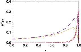
Figure 2: Probability of photon subtraction as a function of BS transmittance $\tau$. Variance is fixed as $V_{A}=50$ and various plots correspond to 1-PSTMSC (Red dashed), 2-PSTMSC (Orange dotted), 1-PSTMSV (Purple large dashed), 2-PSTMSV (Yellow dash dotted) and TMSV (Black solid).

We evaluate the corresponding variance matrix in terms of the moment generating function defined as (see Appendix C)

$$C_{i,j}^{m,n} =\left\langle x_{1}^{i}p_{1}^{j}x_{2}^{m}p_{2}^{n}\right\rangle$$

$$=\int\frac{dx_{1}dp_{1}}{4\pi}\int\frac{dx_{2}dp_{2}}{4\pi}W_{A_{1}A_{2}^{{}^{\prime}}}^{k}(\xi_{1},\xi_{2})x_{1}^{i}p_{1}^{j}x_{2}^{m}p_{2}^{n}.$$ (6)

We express various moments, e.g., $\langle x_{1}^{l}\rangle$ in a compact notation as $\langle x_{1}^{i}\rangle=C_{i,j}^{m,n}\delta_{i,l}\delta_{j,0}\delta_{m,0}\delta_{n,0}$. A straightforward calculation yields the variance matrix of the $k$-PSTMSC to be of the following form

$$\Sigma_{A_{1}A^{\prime}_{2}}=\begin{pmatrix}V_{A}^{x}&0&V_{C}^{x}&0\\ 0&V_{A}^{p}&0&V_{C}^{p}\\ V_{C}^{x}&0&V_{B}^{x}&0\\ 0&V_{C}^{p}&0&V_{B}^{p}\end{pmatrix},$$ (7)

where $V_{i}^{\xi}$, $i\in\{A,B,C\}$ and $\xi\in\{x,p\}$. After photon subtraction the mode $A^{\prime}_{2}$ is then transmitted to Charlie via a quantum channel.

Step 3: Bob also prepares a TMSC state with variance $V_{B}=V_{A}$ and transmits the mode $B_{2}$ to Charlie.

Step 4: Charlie mixes the two modes $A^{\prime}_{2}$ $B_{2}$ received from Alice and Bob respectively via a BS to obtain output modes $C$ and $D$. He then performs a homodyne measurement of the $x$ quadrature on $C$ and of the $p$ quadrature on $D$. The results of these measurements are declared publicly.

Step 5: Based on the publically declared results, Bob adequately displaces his retained mode $B_{1}$ to $B^{\prime}_{1}$. Consequently, the two modes $A_{1}$ and $B^{\prime}_{1}$ are entangled. Afterwards, both the parties perform heterodyne measurement on the modes $A_{1}$ and $B^{\prime}_{1}$ respectively and get correlated outcomes.

Step 6: Alice and Bob perform information reconciliation and privacy amplification to obtain a secure key string.

II.3 Special cases

We now discuss various special cases of PSTMSC state in the context of CV-MDI-QKD. In particular, we show that several of the earlier results in CV-MDI-QKD, can be obtained as limiting cases of our results on PSTMSC.

In the limit $k\rightarrow 0$, the PSTMSC state simply reduces to the TMSC state. This we achieve by setting $k=0$ and $\tau=1$(Fred’s BS transmittivity) in our expression for the covariance matrix. Since the covariance matrix for TMSC is identical to that of TMSV, the results obtained for the aforementioned case are identical to the ones obtained earlier for TMSV. Thus, our results with PSTMSC in CV-MDI-QKD protocols, in the limit $k=0$, reduces to the earlier results obtained with TMSV Li et al. (2014).

Furthermore, in the limit $d\rightarrow 0$ $\forall$ $k\neq 0$, the covariance matrix of PSTMSC represents photon subtraction on the TMSV state. This specific case has already been studied extensively in several CV-MDI-QKD protocols Huang et al. (2013); Ma et al. (2018). Particularly, the previous result on photon subtraction on TMSV is re-examined as a special case of ours. It has also been shown that a non-Gaussian post-selection of data is equivalent to PSTMSV Zhao et al. (2018); Li et al. (2016). This implies that our results, in the limit $d\rightarrow 0$, subsume the earlier results on non-Gaussian CV-MDI-QKD with either photon subtraction on TMSV or non-Gaussian post-selection. For the rest of the paper, while quoting and graphically representing results for states other than PSTMSC, we indeed use the limiting process described above on our more general state.

III Eavesdropping, channel parameters and secure key rate

The protocol described above requires two quantum channels and one classical channel. We assume that an eavesdropper, Eve, performs an entangling cloner attack on each of the quantum channels. The attacks can be correlated with each other, which is known as a two mode attack. However, since the two channels are assumed to be non-interacting and well separated, the correlated attack reduces to two independent one-mode collective attacks on each channel. Under the aforementioned strategy of Eve, the maximum information gained by her on the key will be bounded by the Holevo bound, $\chi_{BE}$. We note that the attack considered above is not optimal.

In the following we provide an analysis of various channel parameters which will be used to calculate the final secret key. We assume that the two channels have transmittance $T_{A}$ and $T_{B}$, given as,

$$T_{A}=10^{-l\frac{L_{AC}}{10}}\quad\text{and}\quad T_{B}=10^{-l\frac{L_{BC}}{10}},$$ (8)

where $l=0.2$dB/Km is the channel loss. Throughout the main text we consider two cases:

Symmetric: In this case we consider $L_{AC}=L_{BC}$, implying Charlie sits midway between Alice and Bob. The total transmission length in this case is $L=2L_{AC}$ with $T_{A}=T_{B}$.

Asymmetric: In this case, $L_{BC}=0$, implying Bob and Charlie are at the same place. The total transmission length then becomes $L=L_{AC}=L_{AB}$ with $T_{B}=1$.

Bob is the only party who displaces his state and his outcomes are taken as the reference key to which Alice reconciles. Due to this inherent asymmetry in the protocol itself the two cases above give very different results.

We can define a normalized parameter $T$ associated with channel transmittance in terms of the only channel parameter $T_{A}$ as

$$T=\frac{T_{A}g^{2}}{2},$$ (9)

where $g$ is the gain of Bob’s displacement operation. The total channel added noise can then be defined as

$$\chi_{line}=\frac{1-T}{T}+\varepsilon_{th},$$ (10)

where $\varepsilon_{th}$ is the thermal excess noise in the equivalent one-way protocol, calculated as given in Ma et al. (2018) and written as

$$\varepsilon_{th}=\frac{T_{B}}{T_{A}}\left(\varepsilon_{B}-2\right)+\varepsilon_{A}+\frac{2}{T_{A}},$$ (11)

where $\varepsilon_{A}$ and $\varepsilon_{B}$ correspond to thermal excess noise in the respective quantum channels and the gain is taken to be as

$$g=\sqrt{\frac{2\left(V_{A}-1\right)}{T_{B}\left(V_{A}+1\right)}},$$ (12)

in order to minimize $\varepsilon_{th}$.

We also assume that Charlie’s homodyne detectors are noisy, with excess noise given as

$$\chi_{homo}=\frac{v_{el}+1-\eta}{\eta},$$ (13)

where, $v_{el}$ is the electric noise of the detectors and $\eta$ is the efficiency. Therefore, the total noise added because of the channel and detectors is

$$\chi_{tot}=\chi_{line}+\frac{2\chi_{homo}}{T_{A}}.$$ (14)

The analysis we present in the following sections is for perfect homodyne detection by Charlie, i.e. $\chi_{homo}=0$, while in Sec. IV.4 we explicitly discuss the tradeoff between Charlie’s noise, secure key rate and total transmission length.

The secure key rate when Eve is assumed to perform a one-mode collective attack on each quantum channel and under the aforementioned channel parameters is given as

$$K=P^{k}_{PS}\left(\beta I_{AB}-\chi_{BE}\right),$$ (15)

where $I_{AB}$ is the mutual information between Alice and Bob and $\chi_{BE}$ is the Holevo bound between Bob and Eve, which characterizes Eve’s maximal information on Bob’s outcomes. It is our intent to optimize various parameters for maximum secure key rate $K$, while the rest are kept fixed throughout the analysis.

The covariance matrix corresponding to the state $\rho_{A_{1}B^{\prime}_{1}}$ which is obtained after Step 5. of the protocol given in Section II.2 is

$$\Sigma_{A_{1}B^{\prime}_{1}}=\begin{pmatrix}V_{A}^{x}&0&\sqrt{T}V_{C}^{x}&0\\ 0&V_{A}^{p}&0&\sqrt{T}V_{C}^{p}\\ \sqrt{T}V_{C}^{x}&0&TV^{\prime x}_{B}&0\\ 0&\sqrt{T}V_{C}^{p}&0&TV^{\prime p}_{B}\end{pmatrix},$$ (16)

where $V^{\prime\xi}_{B}=V^{\xi}_{B}+\chi_{tot}I_{2}$ and $V_{B}^{\xi}$ is the variance of $\xi\in\{x,p\}$ quadrature for Bob’s state.. The mutual information between Alice and Bob, $I_{AB}$ can then be calculated as,

$$I_{AB}=\frac{1}{2}\log_{2}\left(\frac{V_{A_{M}}^{x}}{V_{A_{M}|B_{M}}^{x}}\right)+\frac{1}{2}\log_{2}\left(\frac{V_{A_{M}}^{p}}{V_{A_{M}|B_{M}}^{p}}\right),$$ (17)

such that,

$$V_{A_{M}}^{\xi}=\frac{V_{A}^{\xi}+1}{2},$$ (18)

where $V_{A_{M}|B_{M}}^{\xi}$ is the conditional variance of Alice’s outcome conditioned on Bob’s outcome of his heterodyne measurement and is given as,

$$V_{A_{M}|B_{M}}^{\xi}=\frac{V_{A|B}^{\xi}+1}{2},$$ (19)

where,

$$V_{A|B}^{\xi}=V_{A}^{\xi}-V_{C}^{\xi}\left(V_{B}^{\xi}+I_{2}\right)^{-1}(V_{C}^{\xi})^{T}.$$ (20)

In order to calculate the upper bound of the information obtained by Eve, we assume that she also has access to Fred’s mode $F$ and her state is then given by $\rho_{EF}$. We also assume that she can purify $\rho_{A_{1}B^{\prime}_{1}EF}$. The Holevo bound $\chi_{BE}$ between Bob and Eve can then be calculated as,

$$\chi_{BE} =S(\rho_{EF})-\int dm_{B}p(m_{B})S(\rho_{EF}^{m_{B}})$$ (21)

$$=S(\rho_{A_{1}B^{\prime}_{1}})-S(\rho_{A_{1}}^{m_{B^{\prime}_{1}}}),$$

where $S(\rho)$ is the von-Neumann entropy of the state $\rho$, $m_{B}$ represents measurement outcomes of Bob with probability density $p(m_{B})$ and $\rho_{EF}^{m_{B}}$ is the state of Eve conditioned on Bob’s outcome. The covariance matrices corresponding to the states $\rho_{A_{1}B^{\prime}_{1}}$ and $\rho_{A_{1}}^{m_{B^{\prime}_{1}}}$ are represented by $\Sigma_{A_{1}B^{\prime}_{1}}$ and $\Sigma_{A_{1}}^{m_{B^{\prime}_{1}}}$ respectively. The von-Neumann entropy $S(\rho_{A_{1}B^{\prime}_{1}})$ and $S(\rho_{A_{1}}^{m_{B^{\prime}_{1}}})$ are functions of symplectic eigenvalues $\lambda_{1}$, $\lambda_{2}$ of $\Sigma_{A_{1}B^{\prime}_{1}}$ and $\lambda_{3}$ of $\Sigma_{A_{1}}^{m_{B^{\prime}_{1}}}$ which are given as,

$$S(\rho_{A_{1}B^{\prime}_{1}})=G\left[\frac{\lambda_{1}-1}{2}\right]+G\left[\frac{\lambda_{2}-1}{2}\right],$$ (22)

and

$$S(\rho_{A_{1}}^{m_{B^{\prime}_{1}}})=G\left[\frac{\lambda_{3}-1}{2}\right],$$ (23)

with,

$$G(x)=(x+1)\log_{2}(x+1)-x\log_{2}x,$$ (24)

is the von-Neumann entropy of the thermal state.

IV Simulation results

Having described the protocol in its generality, in this section we provide numerical results corresponding to optimization of some parameters while the rest are kept fixed. We provide the analysis for both the symmetric and asymmetric case, respectively.

It was shown in Ma et al. (2018) that photon subtraction on a TMSV state can lead to an increase in transmission distances for secure key rate for QKD, especially in the extreme asymmetric case, where distances can reach up to $60-70$ kms approximately as compared to $40-50$ kms achievable using only TMSV. In the following subsections we show that performing photon subtraction on a TMSC state can lead to a much better performance as compared to TMSV.

IV.1 Effect of displacement on distance for a fixed key rate

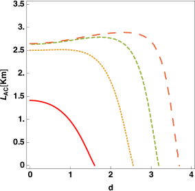
Figure 3: Plots of $L_{AC}$ as a function of vacuum state displacement $d$ for different values of the secret key for the symmetric case with one photon subtraction. The different values of the fixed secret key rate are be $K=10^{-1}$ (Red solid), $K=10^{-2}$ (Tiny dashed), $K=10^{-3}$ (Dashed) and $K=10^{-4}$ (large dashed). The total transmission length is $L=2L_{AC}$. The other parameters are fixed as $V_{A}=50$, $\eta=1$, $\varepsilon_{A}^{th}=0.002=\varepsilon_{B}^{th}$ and $\beta=96\%$.

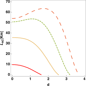
Figure 4: Plots of $L_{AC}$ as a function of vacuum state displacement $d$ for different values of the fixed secret key for the extreme asymmetric case with one photon subtraction. The different values of the fixed secret key rates are $K=10^{-1}$ (Red solid), $K=10^{-2}$ (Tiny dashed), $K=10^{-3}$ (Dashed) and $K=10^{-4}$ (large dashed). The total transmission length is $L=L_{AC}$ and parameters are fixed as $V_{A}=50$, $\varepsilon_{A}^{th}=0.002=\varepsilon_{B}^{th}$ and $\beta=96\%$.

Photon subtraction on TMSV state is known to increase transmission distances. We show that transmission distances can be further improved if we consider PSTMSC state. We explore the variation of distance with displacement for symmetric as well extreme asymmetric case for several fixed values of the key rate. The results are shown in Figs. 3 and 4.

For the symmetric case, we find that a secure key rate of $10^{-4}$ bits/pulse can be achieved for $0.5$ kms more than what was possible for PSTMSV and is shown in Fig. 3. A much more significant improvement of approximately $10$ kms is possible in the asymmetric case for the same key rate as shown in Fig. 4.

Both Fig. 3 and Fig. 4 imply an increase in transmission distance with an increase in coherence with a much more significant difference in the extreme asymmetric case. We find that setting the coherence, $d=2$, transmission lengths can be significantly improved. However, it is also seen that larger coherence values are detrimental to the protocol.

IV.2 Effect of Variance on key rate for a fixed distance

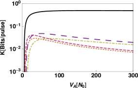
Figure 5: Secret key rate as a function of $V_{A}$ in the symmetric case where $L_{AC}=L_{BC}=2$ kms and total transmission distance $L=2L_{AC}$. Parameters are fixed as: $\tau=0.9$, $\varepsilon_{A}^{th}=0.002=\varepsilon_{B}^{th}$, $\beta=96\%$ and displacement $d=2$. Various curves correspond to $1$-PSTMSC (Red dashed), $2$-PSTMSC (Orange dotted), $1$-PSTMSV (Purple large dashed), $2$-PSTMSV (Yellow dash dotted) and TMSV (Black solid).

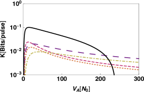
Figure 6: Secret key rate as a function of $V_{A}$ in the asymmetric case where $L_{AC}=20$ kms, $L_{BC}=0$ and total transmission distance $L=L_{AC}$. Parameters are fixed as: $\tau=0.9$, $\varepsilon_{A}^{th}=0.002=\varepsilon_{B}^{th}$, $\beta=96\%$ and displacement $d=2$. Various curves correspond to $1$-PSTMSC (Red dashed), $2$-PSTMSC (Orange dotted), $1$-PSTMSV (Purple large dashed), $2$-PSTMSV (Yellow dash dotted) and TMSV (Black solid).

Like coherence and optimal transmittivity of photon subtraction, choice of variance also plays a vital role in CV-MDI-QKD. In Fig. 5 and Fig. 6 we plot secure key rate as a function of variance of Alice’s PSTMSC state while keeping all the other parameters fixed. We see that for a fixed transmission length $L_{AB}=4$ kms in the symmetric case, the TMSV state outperforms all the other states including PSTMSC. It is also seen that PSTMSV state can achieve a higher secure key rate than PSTMSC for a fixed length and variance. In the extreme asymmetric case, where we fix length $L_{AB}=L_{AC}=20$ kms, the TMSV state still outperforms the other states in terms of higher secure key rate for lower variance. However, for variances larger than $250$, the other states including PSTMSV and PSTMSC outperform TMSV. It is also seen that for extremely small value of variance, PSTMSC state provides a slightly higher key rate than PSTMSV. However, we find that a small value of variance, $V_{A}=50$, is enough in order to optimize the protocol for longer transmission lengths.

IV.3 Effect of Length on key rate

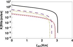
Figure 7: Secret key rate as a function of $L_{AC}$ in the symmetric case where $L_{AC}=L_{BC}$, $V_{A}=50$ and total transmission distance $L=2L_{AC}$. Parameters are fixed as: $\tau=0.9$, $\varepsilon_{A}^{th}=0.002=\varepsilon_{B}^{th}$, $\beta=96\%$ and coherence $d=2$. Various curves correspond to $1$-PSTMSC (Red dashed), $2$-PSTMSC (Orange dotted), $1$-PSTMSV (Purple large dashed), $2$-PSTMSV (Yellow dash dotted) and TMSV (Black solid).

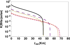
Figure 8: Secret key rate as a function of $L_{AC}$ in the asymmetric case where $L_{BC}=0$, $V_{A}=50$ and total transmission distance $L=L_{AC}$. Parameters are fixed as: $\tau=0.9$, $\varepsilon_{A}^{th}=0.002=\varepsilon_{B}^{th}$, $\beta=96\%$ and displacement $d=2$. Various curves correspond to $1$-PSTMSC (Red dashed), $2$-PSTMSC (Orange dotted), $1$-PSTMSV (Purple large dashed), $2$-PSTMSV (Yellow dash dotted) and TMSV (Black solid).

Equipped with approximate values of $\tau$, $a$ and $V_{A}$ that maximize transmission distance for PSTMSC, we plot key rate as a function of $L_{AC}$ in Fig. 7 and Fig. 8 corresponding to symmetric and extreme asymmetric case respectively. In the symmetric case the total transmission distance is given by $L_{AB}=2L_{AC}$, while in the extreme asymmetric case, $L_{AB}=L_{AC}$.

We find that for the symmetric case TMSV state offers better results than any other state in terms of both key rate and transmission distance. However, for the same case it is seen that PSTMSC state offers a longer transmission length than PSTMSV while the maximum key rate achievable by the former is less than the latter.

The advantage of using PSTMSC is apparent in the extreme asymmetric case where it significantly outperforms the others by approximately $10$ kms while its maximum achievable key rate is still the least.

From the above it is clear that a small amount of coherence is actually favorable if maximizing the transmission distance. Although offering lesser key rate, PSTMSC state can drastically increase the distances upto which QKD can be performed. Furthermore, real experiments rarely deal with squeezed vacuum states which are also harder to prepare than squeezed coherent states. Our results make it evident that it is highly advantageous if a squeezed coherent light source is used instead of squeezed vacuum.

IV.4 Noisy homodyne detectors

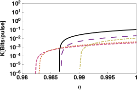
Figure 9: Secret key rate as a function of $\eta$ in the asymmetric case where $L_{AC}=20$ kms and $V_{A}=50$ with total transmission distance $L=L_{AC}$. Parameters are fixed as: $\tau=0.9$, $\varepsilon_{A}^{th}=0.002=\varepsilon_{B}^{th}$, $\beta=96\%$, displacement $d=2$ and $\nu_{el}=0.01$. Various curves correspond to $1$-PSTMSC (Red dashed), $2$-PSTMSC (Orange dotted), $1$-PSTMSV (Purple large dashed), $2$-PSTMSV (Yellow dash dotted) and TMSV (Black solid).

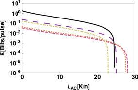
Figure 10: Secret key rate as a function of $L_{AC}$ in the asymmetric case where $V_{A}=50$ and total transmission distance $L=L_{AC}$. Parameters are fixed as: $\tau=0.9$, $\varepsilon_{A}^{th}=0.002=\varepsilon_{B}^{th}$, $\beta=96\%$, displacement $d=2$ and detector efficiency $\eta=0.995$. Various curves correspond to $1$-PSTMSC (Red dashed), $2$-PSTMSC (Orange dotted), $1$-PSTMSV (Purple large dashed), $2$-PSTMSV (Yellow dash dotted) and TMSV (Black solid).

Noise and efficiency of Charlie’s homodyne detection also plays a major role in optimizing the total transmission length of the protocol. We find that the efficiency of the detectors needs to be close to unity to maintain transmission lengths upto $30$ kms as is evident in Fig. 10. A drastic drop of approximately $30$ kms in the transmission length is observed for even a small detector inefficiency of $\eta=0.995$ and $\nu_{el}=0.01$. Furthermore, the range for tolerable detector efficiency $\eta$ can be made as low as $86\%$ for smaller transmission distances. From Fig. 9 it is also seen that PSTMSC state is more robust than PSTMSV and TMSV against detection inefficiencies which is also evident in Fig. 10.

V Conclusion

In this paper we showed that PSTMSC states have an advantage over PSTMSV in terms of the distance over which QKD can be carried out. To that end we explicitly derive the covariance matrix for PSTMSC state, which to the best of our knowledge has not been attempted before. Using the same in CV-MDI-QKD, we find that for perfect homodyne detectors, and a small amount of coherence $d=2$, the transmission distances can be made as large as $70$ kms in the extreme asymmetric case which is considerably longer than what is achievable with PSTMSV. However, the same effects are not noticeable in the symmetric case. We also find that transmission distances of PSTMSC MDI QKD can achieve a maximum value of $30$ kms under noisy homodyne detectors of Charlie, which is suitable for a small metropolitan city. This distance is again significantly higher than what can be achieved with PSTMSV with noisy homodyne detectors, implying that PSTMSC is a better candidate for long distance CV-MDI-QKD. Furthermore, we showed that many of the previous results of CV-MDI-QKD can be obtained as limiting cases of the PSTMSC based CV-MDI-QKD protocol. We emphasize that, while non-Gaussian operations on TMSV have been well studied, the same is not true for TMSC states. The covariance matrix computed here is expected to be useful to characterize the properties of such states and will find further application in various information processing tasks.

Appendix A Wigner Distribution for $k$-PSTMSC state

Figure 11: A TMSC state is passed through the modes $A_{1}$ $A_{2}$ while mode $F_{0}$ is initialized to vacuum $|0\rangle\langle 0|$. Photon number resolving detector (PNRD) given by the POVM $\{\Pi,\mathds{1}-\Pi\}$, where $\Pi=|n\rangle\langle n|$ is applied to mode $F_{0}$.

In this section we provide detailed calculations for evaluating the Wigner distribution for $k$-PSTMSC state. We start with a TMSC state and a third mode initialized to the vacuum state. After mixing the vacuum state with one of the modes of TMSC by the use of a BS, we perform a $k$ photon number detection on the third mode. Consequently, the TMSC state is then transformed to a $k$-PSTMSC. The basic schematic of photon subtraction on a TMSC is shown in Fig. 11.

We start with the Wigner distribution for TMSC. In shot noise unit (SNU), for a two-mode squeezed coherent state (TMSC), i.e., $\rho_{A_{1}A_{2}}=S_{ab}(r)\left|d,d\right\rangle$, with $S_{ab}(r)=e^{r(a^{\dagger}b^{\dagger}-ab)}$, its Wigner distribution is given by

$$W_{A_{1}A_{2}}(\xi_{1},\xi_{2})=4e^{-d^{2}}e^{-\frac{\mu^{2}+\nu^{2}}{2}(x_{1}^{2}+p_{1}^{2}+x_{2}^{2}+p_{2}^{2})+2\mu\nu(x_{1}x_{2}-p_{1}p_{2})+d(\mu-\nu)(x_{1}+x_{2})},$$ (25)

where $\mu=\cosh r$ and $\nu=\sinh r$ and the normalization is given by $\int\frac{dx_{1}dp_{1}}{4\pi}\int\frac{dx_{2}dp_{2}}{4\pi}W_{\rm{A_{1}A_{2}}}(\xi_{1},\xi_{2})=1$ such that $\xi_{i}=\{x_{i},p_{i}\}$ ($i=1,2$). On the other hand, Wigner distribution for a single mode photon number state is given by

$$W^{n}(\xi) =2(-1)^{n}e^{-\frac{x^{2}+p^{2}}{2}}L_{n}(x^{2}+p^{2})$$

$$=\frac{2(-1)^{n}e^{-\frac{x^{2}+p^{2}}{2}}}{n!}\partial^{n}_{\eta}\partial^{n}_{\zeta}\left[e^{\eta\zeta+(x+ip)\eta-(x-ip)\zeta}\right]_{\begin{subarray}{c}\eta=0\\ \zeta=0\end{subarray}},$$ (26)

where $L_{n}(x)$ is the Laguerre polynomial. Wigner Distribution for the vacuum ($W^{0}(\xi)$) could be trivially obtained by setting $n=0$.

The tripartite Wigner distribution for Alice, Bob in TMSC and Fred in vacuum is given by $W_{A_{1}A_{2}F_{0}}(\xi_{1},\xi_{2},\xi_{3})=W_{A_{1}A_{2}}(\xi_{1},\xi_{2})W_{F_{0}}^{0}(\xi_{3})$. Let’s consider the mixing of modes ”$A_{2}$” and ”$F$” through BS with transmittivity $\tau$ for which quadrature variables transform as $\begin{pmatrix}\xi_{2}\\ \xi_{3}\end{pmatrix}\rightarrow\begin{pmatrix}\xi^{{}^{\prime}}_{2}\\ \xi^{{}^{\prime}}_{3}\end{pmatrix}=S_{\rm{BS}}\begin{pmatrix}\xi_{2}\\ \xi_{3}\end{pmatrix}$, where

$$S_{\rm{BS}}=\begin{pmatrix}\sqrt{\tau}&0&\sqrt{1-\tau}&0\\ 0&\sqrt{\tau}&0&\sqrt{1-\tau}\\ -\sqrt{1-\tau}&0&\sqrt{\tau}&0\\ 0&-\sqrt{1-\tau}&0&\sqrt{\tau}\end{pmatrix}$$ (27)

is the BS transformation matrix. It is well-known that under a linear canonical transformation of the quadrature variables $\xi\rightarrow\xi^{{}^{\prime}}=S\xi$, Wigner distribution changes as $S:W(\xi)\rightarrow W(S^{-1}\xi)$. Consequently, under BS mixing input Wigner distribution $W_{A_{1}A_{2}F_{0}}(\xi_{1},\xi_{2},\xi_{3})$ changes as,

$$W_{A_{1}A_{2}F_{0}}(\xi_{1},\xi_{2},\xi_{3}) \xrightarrow{\rm{BS}}W_{A_{1}A^{{}^{\prime}}_{2}F_{1}}(\xi_{1},\xi_{2},\xi_{3})$$

$$=8e^{-d^{2}}e^{-\frac{\mu^{2}+\nu^{2}}{2}(x_{1}^{2}+p_{1}^{2})+d(\mu-\nu)x_{1}}e^{-\frac{\mu^{2}-(1-2\tau)\nu^{2}}{2}(x_{2}^{2}+p_{2}^{2})+2\mu\nu\sqrt{\tau}(x_{1}x_{2}-p_{1}p_{2})+d\sqrt{\tau}(\mu-\nu)x_{2}}~{}\times$$

$$~{}~{}~{}~{}~{}~{}~{}~{}e^{-\frac{\mu^{2}+(1-2\tau)\nu^{2}}{2}(x_{3}^{2}+p_{3}^{2})+\left(2\nu\sqrt{1-\tau}(\nu\sqrt{\tau}x_{2}-\mu x_{1})-d\sqrt{1-\tau}(\mu-\nu)\right)x_{3}+2\nu\sqrt{1-\tau}(\nu\sqrt{\tau}p_{2}+\mu p_{1})p_{3}}.$$ (28)

The Wigner distribution for $k$-PSTMSC can then be written as,

$$\tilde{W}_{A_{1}A^{{}^{\prime}}_{2}}^{k}(\xi_{1},\xi_{2}) =\int\frac{dx_{3}dp_{3}}{4\pi}~{}W_{A_{1}A^{{}^{\prime}}_{2}F_{1}}(\xi_{1},\xi_{2},\xi_{3})~{}W_{F_{1}}^{k}(\xi_{3})$$

$$=16\frac{(-1)^{k}}{k!}e^{-d^{2}}e^{-\frac{\mu^{2}+\nu^{2}}{2}(x_{1}^{2}+p_{1}^{2})+d(\mu-\nu)x_{1}}e^{-\frac{\mu^{2}-(1-2\tau)\nu^{2}}{2}(x_{2}^{2}+p_{2}^{2})+2\mu\nu\sqrt{\tau}(x_{1}x_{2}-p_{1}p_{2})+d\sqrt{\tau}(\mu-\nu)x_{2}}~{}\partial^{k}_{\eta}\partial^{k}_{\zeta}\Big{[}e^{\eta\zeta}~{}\times$$

$$~{}~{}~{}\int\frac{dx_{3}dp_{3}}{4\pi}e^{-(\mu^{2}-\tau\nu^{2})(x_{3}^{2}+p_{3}^{2})+\left((\eta-\zeta)+2\nu\sqrt{1-\tau}(\nu\sqrt{\tau}x_{2}-\mu x_{1})-d\sqrt{1-\tau}(\mu-\nu)\right)x_{3}+\left(i(\eta+\zeta)+2\nu\sqrt{1-\tau}(\nu\sqrt{\tau}p_{2}+\mu p_{1})\right)p_{3}}\Big{]}_{\begin{subarray}{c}\eta=0\\ \zeta=0\end{subarray}}$$

$$=\frac{4(-1)^{k}}{k!(\mu^{2}-T\nu^{2})}e^{-d^{2}}e^{-\frac{\mu^{2}+\nu^{2}}{2}(x_{1}^{2}+p_{1}^{2})+d(\mu-\nu)x_{1}}e^{-\frac{\mu^{2}-(1-2\tau)\nu^{2}}{2}(x_{2}^{2}+p_{2}^{2})+2\mu\nu\sqrt{\tau}(x_{1}x_{2}-p_{1}p_{2})+d\sqrt{\tau}(\mu-\nu)x_{2}}~{}\times$$

$$~{}~{}~{}~{}~{}\partial^{k}_{\eta}\partial^{k}_{\zeta}\left[e^{\eta\zeta}e^{\frac{1}{4(\mu^{2}-\tau\nu^{2})}\left\{\left((\eta-\zeta)+2\nu\sqrt{1-\tau}(\nu\sqrt{\tau}x_{2}-\mu x_{1})-d\sqrt{1-\tau}(\mu-\nu)\right)^{2}+\left(i(\eta+\zeta)+2\nu\sqrt{1-\tau}(\nu\sqrt{\tau}p_{2}+\mu p_{1})\right)^{2}\right\}}\right]_{\begin{subarray}{c}\eta=0\\ \zeta=0\end{subarray}}$$

$$=\frac{4(-1)^{k}}{k!(\mu^{2}-\tau\nu^{2})}e^{-d^{2}}e^{-\frac{\mu^{2}+\nu^{2}}{2}(x_{1}^{2}+p_{1}^{2})+d(\mu-\nu)x_{1}}e^{-\frac{\mu^{2}-(1-2\tau)\nu^{2}}{2}(x_{2}^{2}+p_{2}^{2})+2\mu\nu\sqrt{\tau}(x_{1}x_{2}-p_{1}p_{2})+d\sqrt{\tau}(\mu-\nu)x_{2}}~{}\times$$

$$~{}~{}~{}~{}~{}e^{\frac{\nu^{2}(1-\tau)}{\mu^{2}-\tau\nu^{2}}\left\{(\nu\sqrt{\tau}x_{2}-\mu x_{1})^{2}+(\nu\sqrt{\tau}p_{2}+\mu p_{1})^{2}\right\}}e^{\frac{d^{2}(1-\tau)(\mu-\nu)^{2}}{4(\mu^{2}-\tau\nu^{2})}}e^{-\frac{d\nu(\mu-\nu)(1-\tau)}{\mu^{2}-\tau\nu^{2}}(\nu\sqrt{\tau}x_{2}-\mu x_{1})}~{}\times$$

$$~{}~{}~{}~{}~{}\partial^{k}_{\eta}\partial^{k}_{\zeta}\left[e^{\frac{\nu^{2}(1-\tau)}{\mu^{2}-\tau\nu^{2}}\eta\zeta+\frac{\sqrt{1-\tau}}{\mu^{2}-\tau\nu^{2}}\left\{\nu^{2}\sqrt{\tau}(x_{2}+ip_{2})-\mu\nu(x_{1}-ip_{1})-\frac{d(\mu-\nu)}{2}\right\}\eta-\frac{\sqrt{1-\tau}}{\mu^{2}-\tau\nu^{2}}\left\{\nu^{2}\sqrt{\tau}(x_{2}-ip_{2})-\mu\nu(x_{1}+ip_{1})-\frac{d(\mu-\nu)}{2}\right\}\zeta}\right]_{\begin{subarray}{c}\eta=0\\ \zeta=0\end{subarray}}$$

$$=(-A)^{k}W_{A_{1}A_{2}^{{}^{\prime}}}^{0}(\xi_{1},\xi_{2})~{}L_{k}\left(\frac{|\xi_{12}|^{2}}{\nu^{2}(\mu^{2}-\tau\nu^{2})}\right),$$ (29)

where,

$$A =\frac{\nu^{2}(1-\tau)}{(\mu^{2}-\tau\nu^{2})}~{};~{}\xi_{12}=\nu^{2}\sqrt{\tau}(x_{2}+ip_{2})-\mu\nu(x_{1}-ip_{1})-\frac{d(\mu-\nu)}{2}~{}~{}~{}~{}~{}\rm{and}$$

$$W_{A_{1}A_{2}^{{}^{\prime}}}^{0}(\xi_{1},\xi_{2}) =\frac{4}{\mu^{2}-\tau\nu^{2}}e^{-d^{2}}e^{-\frac{\mu^{2}+\nu^{2}}{2}(x_{1}^{2}+p_{1}^{2})-\frac{\mu^{2}-(1-2\tau)\nu^{2}}{2}(x_{2}^{2}+p_{2}^{2})+2\mu\nu\sqrt{\tau}(x_{1}x_{2}-p_{1}p_{2})+d(\mu-\nu)(x_{1}+\sqrt{\tau}x_{2})}e^{\frac{1-\tau}{\mu^{2}-\tau\nu^{2}}|\xi_{12}|^{2}}.$$ (30)

Appendix B Probability for $k$-PSTMSC

In this section we calculate the probability of successfully subtracting $k$ photons from a TMSC state. This probability will also serve as a normalization to the Wigner distribution as derived above.

Probability of $k$-photon subtraction is obtained by integrating the resultant Wigner distribution, i.e., $P(k)=\int\frac{dx_{1}dp_{1}}{4\pi}\int\frac{dx_{2}dp_{2}}{4\pi}W_{A_{1}A_{2}^{{}^{\prime}}}^{k}(\xi_{1},\xi_{2})$. In a straightforward calculation it could be shown that

$$P^{k}_{PS} =(-A)^{k}\int\frac{dx_{1}dp_{1}}{4\pi}\int\frac{dx_{2}dp_{2}}{4\pi}W_{A_{1}A_{2}^{{}^{\prime}}}^{0}(\xi_{1},\xi_{2})~{}L_{k}\left(\frac{|\xi_{12}|^{2}}{\nu^{2}(\mu^{2}-\tau\nu^{2})}\right)$$

$$=\frac{(-1)^{k}}{k!(\mu^{2}-\tau\nu^{2})}e^{-\left(1-\frac{(1-\tau)(\mu-\nu)^{2}}{4(\mu^{2}-\tau\nu^{2})}\right)d^{2}}\partial^{k}_{\eta}\partial^{k}_{\zeta}\Big{[}e^{\frac{\nu^{2}(1-\tau)}{\mu^{2}-\tau\nu^{2}}\eta\zeta-\frac{d(\mu-\nu)\sqrt{1-\tau}}{2(\mu^{2}-\tau\nu^{2})}(\eta-\zeta)}~{}\times$$

$$~{}~{}~{}\int\frac{dx_{1}dp_{1}}{2\pi}e^{-\frac{\mu^{2}+\tau\nu^{2}}{2(\mu^{2}-\tau\nu^{2})}(x_{1}^{2}+p_{1}^{2})+\frac{1}{\mu^{2}-\tau\nu^{2}}\left\{d(\mu-\tau\nu)-\mu\nu\sqrt{1-\tau}(\eta-\zeta)\right\}x_{1}+\frac{i\mu\nu\sqrt{1-\tau}}{\mu^{2}-\tau\nu^{2}}(\eta+\zeta)p_{1}}~{}\times$$

$$~{}~{}~{}\int\frac{dx_{2}}{\sqrt{2\pi}}e^{-\frac{\mu^{2}+\tau\nu^{2}}{2(\mu^{2}-\tau\nu^{2})}x_{2}^{2}+\frac{\sqrt{\tau}}{\mu^{2}-\tau\nu^{2}}\left\{2\mu\nu x_{1}+\nu^{2}\sqrt{1-\tau}(\eta-\zeta)+d(\mu-\nu)\right\}x_{2}}\int\frac{dp_{2}}{\sqrt{2\pi}}e^{-\frac{\mu^{2}+\tau\nu^{2}}{2(\mu^{2}-\tau\nu^{2})}p_{2}^{2}-\frac{\sqrt{\tau}}{\mu^{2}-\tau\nu^{2}}\left\{2\mu\nu p_{1}-i\nu^{2}\sqrt{1-\tau}(\eta+\zeta)\right\}p_{2}}\Big{]}_{\begin{subarray}{c}\eta=0\\ \zeta=0\end{subarray}}$$

$$=\frac{(-1)^{k}}{k!(\mu^{2}-T\nu^{2})}\frac{\mu^{2}-\tau\nu^{2}}{\mu^{2}+\tau\nu^{2}}e^{-\left\{1-\frac{(1-\tau)(\mu-\nu)^{2}}{4(\mu^{2}-\tau\nu^{2})}-\frac{(\mu-\nu)^{2}\tau}{2(\mu^{4}-\tau^{2}\nu^{4})}\right\}d^{2}}\partial^{k}_{\eta}\partial^{k}_{\zeta}\Big{[}e^{\frac{\nu^{2}(1-\tau)}{\mu^{2}+\tau\nu^{2}}\eta\zeta-\frac{d(\mu-\nu)\sqrt{1-\tau}}{2(\mu^{2}+\tau\nu^{2})}(\eta-\zeta)}~{}\times$$

$$~{}~{}~{}\int\frac{dx_{1}}{\sqrt{2\pi}}e^{-\frac{\mu^{2}-\tau\nu^{2}}{2(\mu^{2}+\tau\nu^{2})}x_{1}^{2}+\frac{1}{\mu^{2}+\tau\nu^{2}}\left\{d(\mu+\tau\nu)-\mu\nu\sqrt{1-\tau}(\eta-\zeta)\right\}x_{1}}\int\frac{dp_{1}}{\sqrt{2\pi}}e^{-\frac{\mu^{2}-\tau\nu^{2}}{2(\mu^{2}+\tau\nu^{2})}p_{1}^{2}+\frac{i\mu\nu\sqrt{1-\tau}}{\mu^{2}+\tau\nu^{2}}(\eta+\zeta)p_{1}}\Big{]}_{\begin{subarray}{c}\eta=0\\ \zeta=0\end{subarray}}$$

$$=\frac{(-1)^{k}}{k!(\mu^{2}-\tau\nu^{2})}e^{-\left\{1-\frac{(1-\tau)(\mu-\nu)^{2}}{4(\mu^{2}-\tau\nu^{2})}-\frac{(\mu-\nu)^{2}\tau}{2(\mu^{4}-\tau^{2}\nu^{4})}-\frac{(\mu+\tau\nu)^{2}}{2(\mu^{4}-\tau^{2}\nu^{4})}\right\}d^{2}}~{}\times\partial^{k}_{\eta}\partial^{k}_{\zeta}\left[e^{-\frac{\nu^{2}(1-\tau)}{\mu^{2}-\tau\nu^{2}}\eta\zeta-\frac{d(\mu+\nu)\sqrt{1-\tau}}{2(\mu^{2}-\tau\nu^{2})}\eta+\frac{d(\mu+\nu)\sqrt{1-\tau}}{2(\mu^{2}-\tau\nu^{2})}\zeta}\right]_{\begin{subarray}{c}\eta=0\\ \zeta=0\end{subarray}}$$

$$=\frac{A^{k}}{\mu^{2}-\tau\nu^{2}}e^{-\frac{(1-\tau)(\mu+\nu)^{2}}{4(\mu^{2}-\tau\nu^{2})}d^{2}}L_{k}\left(-\frac{d^{2}(\mu+\nu)^{2}}{4\nu^{2}(\mu^{2}-\tau\nu^{2})}\right).$$ (31)

Thus the normalized Wigner distribution for $k$-PSTMSC is given by

$$W_{A_{1}A^{{}^{\prime}}_{2}}^{k}(\xi_{1},\xi_{2})=\left(P^{k}_{PS}\right)^{-1}\tilde{W}_{A_{1}A^{{}^{\prime}}_{2}}^{k}(\xi_{1},\xi_{2})$$ (32)

Appendix C Co-variance Matrix for $k$-PSTMSC

In this section we derive the co-variance matrix for the $k$-PSTMSC state by using moment generating functions.

The moment generating function for the $k$-PSTMSC is given by

$$C_{i,j}^{m,n} =\left\langle x_{1}^{i}p_{1}^{j}x_{2}^{m}p_{2}^{n}\right\rangle=\frac{1}{P^{k}_{PS}}\int\frac{dx_{1}dp_{1}}{4\pi}\int\frac{dx_{2}dp_{2}}{4\pi}\tilde{W}_{A_{1}A_{2}^{{}^{\prime}}}^{k}(\xi_{1},\xi_{2})x_{1}^{i}p_{1}^{j}x_{2}^{m}p_{2}^{n}$$

$$=\frac{1}{P^{k}_{PS}}\partial_{a}^{i}\partial_{b}^{j}\partial_{s}^{m}\partial_{t}^{n}\left[\int\frac{dx_{1}dp_{1}}{4\pi}\int\frac{dx_{2}dp_{2}}{4\pi}\tilde{W}_{A_{1}A_{2}^{{}^{\prime}}}^{k}(\xi_{1},\xi_{2})e^{ax_{1}+bp_{1}+sx_{2}+tp_{2}}\right]_{\begin{subarray}{c}a=0,b=0\\ s=0,t=0\end{subarray}}$$

$$=\frac{1}{P^{k}_{PS}}\frac{(-1)^{k}}{k!(\mu^{2}-\tau\nu^{2})}e^{-\left(1-\frac{(1-\tau)(\mu-\nu)^{2}}{4(\mu^{2}-\tau\nu^{2})}\right)d^{2}}\partial_{a}^{i}\partial_{b}^{j}\partial_{s}^{m}\partial_{t}^{n}\partial^{k}_{\eta}\partial^{k}_{\zeta}\Big{[}e^{\frac{\nu^{2}(1-\tau)}{\mu^{2}-\tau\nu^{2}}\eta\zeta-\frac{d(\mu-\nu)\sqrt{1-\tau}}{2(\mu^{2}-\tau\nu^{2})}(\eta-\zeta)}~{}\times$$

$$~{}~{}~{}\int\frac{dx_{1}dp_{1}}{2\pi}e^{-\frac{\mu^{2}+\tau\nu^{2}}{2(\mu^{2}-\tau\nu^{2})}(x_{1}^{2}+p_{1}^{2})+\frac{1}{\mu^{2}-\tau\nu^{2}}\left\{d(\mu-\tau\nu)-\mu\nu\sqrt{1-\tau}(\eta-\zeta)+a(\mu^{2}-\tau\nu^{2})\right\}x_{1}+\left\{\frac{i\mu\nu\sqrt{1-\tau}}{\mu^{2}-\tau\nu^{2}}(\eta+\zeta)+b\right\}p_{1}}~{}\times$$

$$~{}~{}~{}~{}\int\frac{dx_{2}}{\sqrt{2\pi}}e^{-\frac{\mu^{2}+\tau\nu^{2}}{2(\mu^{2}-\tau\nu^{2})}x_{2}^{2}+\frac{\sqrt{\tau}}{\mu^{2}-\tau\nu^{2}}\left\{2\mu\nu x_{1}+\nu^{2}\sqrt{1-\tau}(\eta-\zeta)+d(\mu-\nu)+s\frac{\mu^{2}-\tau\nu^{2}}{\sqrt{\tau}}\right\}x_{2}}$$

$$~{}~{}~{}\int\frac{dp_{2}}{\sqrt{2\pi}}e^{-\frac{\mu^{2}+\tau\nu^{2}}{2(\mu^{2}-\tau\nu^{2})}p_{2}^{2}-\frac{\sqrt{\tau}}{\mu^{2}-\tau\nu^{2}}\left\{2\mu\nu p_{1}-i\nu^{2}\sqrt{1-\tau}(\eta+\zeta)-t\frac{\mu^{2}-\tau\nu^{2}}{\sqrt{\tau}}\right\}p_{2}}\Big{]}_{\begin{subarray}{c}a=0,b=0,\eta=0\\ s=0,t=0,\zeta=0\end{subarray}}$$

$$=\frac{1}{P^{k}_{PS}}\frac{(-1)^{k}}{k!(\mu^{2}+\tau\nu^{2})}e^{-\left\{1-\frac{(1-\tau)(\mu-\nu)^{2}}{4(\mu^{2}-\tau\nu^{2})}-\frac{(\mu-\nu)^{2}\tau}{2(\mu^{4}-\tau^{2}\nu^{4})}\right\}d^{2}}\partial_{a}^{i}\partial_{b}^{j}\partial_{s}^{m}\partial_{t}^{n}\Big{[}e^{\frac{d(\mu-\nu)\sqrt{\tau}}{\mu^{2}+\tau\nu^{2}}c+\frac{\mu^{2}-\tau\nu^{2}}{2(\mu^{2}+\tau\nu^{2})}\left(s^{2}+t^{2}\right)}~{}\times$$

$$~{}~{}~{}\partial^{k}_{\eta}\partial^{k}_{\zeta}\Big{[}e^{\frac{\nu^{2}(1-\tau)}{\mu^{2}+\tau\nu^{2}}\eta\zeta-\left\{\frac{d(\mu-\nu)\sqrt{1-\tau}}{2(\mu^{2}+\tau\nu^{2})}-\frac{\nu^{2}\sqrt{\tau(1-\tau)}}{\mu^{2}+\tau\nu^{2}}s\right\}(\eta-\zeta)+\frac{i\nu^{2}t\sqrt{\tau(1-\tau)}}{\mu^{2}+\tau\nu^{2}}(\eta+\zeta)}~{}\times$$

$$~{}~{}~{}\int\frac{dx_{1}}{\sqrt{2\pi}}e^{-\frac{\mu^{2}-\tau\nu^{2}}{2(\mu^{2}+\tau\nu^{2})}x_{1}^{2}+\frac{1}{\mu^{2}+\tau\nu^{2}}\left\{d(\mu+\tau\nu)-\mu\nu\sqrt{1-\tau}(\eta-\zeta)+a(\mu^{2}+\tau\nu^{2})+2\mu\nu\sqrt{\tau}s\right\}x_{1}}\times$$

$$~{}~{}~{}~{}\int\frac{dp_{1}}{\sqrt{2\pi}}e^{-\frac{\mu^{2}-\tau\nu^{2}}{2(\mu^{2}+\tau\nu^{2})}p_{1}^{2}+\frac{\mu\nu}{\mu^{2}+\tau\nu^{2}}\left\{i\sqrt{1-\tau}(\eta+\zeta)-2\sqrt{\tau}t+b\frac{\mu^{2}+\tau\nu^{2}}{\mu\nu}\right\}p_{1}}\Big{]}_{\begin{subarray}{c}\eta=0\\ \zeta=0\end{subarray}}\Big{]}_{\begin{subarray}{c}a=0,b=0\\ s=0,t=0\end{subarray}}$$

$$=\frac{1}{P^{k}_{PS}}\frac{(-1)^{k}}{k!(\mu^{2}-\tau\nu^{2})}e^{-\frac{(1-\tau)(\mu+\nu)^{2}}{4(\mu^{2}-\tau\nu^{2})}d^{2}}~{}\times\partial_{a}^{i}\partial_{b}^{j}\partial_{s}^{m}\partial_{t}^{n}\Big{[}e^{\frac{\mu^{2}+\tau\nu^{2}}{2(\mu^{2}-\tau\nu^{2})}\left(a^{2}+b^{2}+s^{2}+t^{2}\right)+\frac{2\mu\nu\sqrt{\tau}}{\mu^{2}-\tau\nu^{2}}(as-bt)}~{}\times$$

$$~{}~{}~{}e^{\frac{\mu+\tau\nu}{\mu^{4}-\tau^{2}\nu^{4}}\left\{a(\mu^{2}+\tau\nu^{2})+2\mu\nu\sqrt{\tau}s\right\}d}~{}\times\partial^{k}_{\eta}\partial^{k}_{\zeta}\left[e^{-\frac{\nu^{2}(1-\tau)}{\mu^{2}-\tau\nu^{2}}\eta\zeta}e^{-\frac{Z\sqrt{1-\tau}}{2(\mu^{2}-\tau\nu^{2})}\eta+\frac{Z^{*}\sqrt{1-\tau}}{2(\mu^{2}-\tau\nu^{2})}\zeta}\right]_{\begin{subarray}{c}\eta=0\\ \zeta=0\end{subarray}}\Big{]}_{\begin{subarray}{c}a=0,b=0\\ s=0,t=0\end{subarray}}$$

$$=\frac{1}{L_{k}\left(-\frac{d^{2}(\mu+\nu)^{2}}{4\nu^{2}(\mu^{2}-\tau\nu^{2})}\right)}\partial_{a}^{i}\partial_{b}^{j}\partial_{s}^{m}\partial_{t}^{n}\Big{[}e^{\frac{\mu^{2}+\tau\nu^{2}}{2(\mu^{2}-\tau\nu^{2})}\left(a^{2}+b^{2}+s^{2}+t^{2}\right)+\frac{2\mu\nu\sqrt{\tau}}{\mu^{2}-\tau\nu^{2}}(as-bt)+\frac{\mu+\tau\nu}{\mu^{4}-\tau^{2}\nu^{4}}\left\{a(\mu^{2}+\tau\nu^{2})+2\mu\nu\sqrt{\tau}s\right\}d}~{}\times$$

$$~{}~{}~{}~{}~{}~{}~{}~{}~{}~{}~{}~{}~{}~{}~{}~{}~{}~{}~{}~{}~{}~{}~{}~{}~{}~{}~{}~{}~{}~{}~{}~{}~{}~{}~{}~{}~{}~{}~{}~{}~{}~{}~{}~{}L_{k}\left(-\frac{|Z|^{2}}{4\nu^{2}(\mu^{2}-\tau\nu^{2})}\right)\Big{]}_{\begin{subarray}{c}a=0,b=0\\ s=0,t=0\end{subarray}},$$ (33)

where $Z=d(\mu+\nu)+2\mu\nu(a-ib)+2\sqrt{\tau}\nu^{2}(s+it)$. We express various moments, e.g., $\langle x_{1}^{l}\rangle$ in a compact notation as $\langle x_{1}^{i}\rangle=C_{i,j}^{m,n}\delta_{i,l}\delta_{j,0}\delta_{m,0}\delta_{n,0}$. This easily leads to,

$$\left\langle x_{1}\right\rangle =C_{i,j}^{m,n}\delta_{i,1}\delta_{j,0}\delta_{m,0}\delta_{n,0}$$

$$=\frac{1}{L_{k}\left(-\frac{d^{2}(\mu+\nu)^{2}}{4\nu^{2}(\mu^{2}-\tau\nu^{2})}\right)}\partial_{a}\left[e^{\frac{\mu^{2}+\tau\nu^{2}}{2(\mu^{2}-\tau\nu^{2})}a^{2}+\frac{d(\mu+\tau\nu)}{\mu^{2}-\tau\nu^{2}}a}~{}\times L_{k}\left(-\frac{(d(\mu+\nu)+2\mu\nu a)^{2}}{4\nu^{2}(\mu^{2}-\tau\nu^{2})}\right)\right]_{a=0}$$

$$=\frac{d(\mu+\tau\nu)}{\mu^{2}-\tau\nu^{2}}+\frac{d\mu(\mu+\nu)}{\nu(\mu^{2}-\tau\nu^{2})}\frac{L_{k-1}^{1}\left(-\frac{d^{2}(\mu+\nu)^{2}}{4\nu^{2}(\mu^{2}-\tau\nu^{2})}\right)}{L_{k}\left(-\frac{d^{2}(\mu+\nu)^{2}}{4\nu^{2}(\mu^{2}-\tau\nu^{2})}\right)}$$ (34a)

$$\left\langle x_{1}^{2}\right\rangle =C_{i,j}^{m,n}\delta_{i,2}\delta_{j,0}\delta_{m,0}\delta_{n,0}$$

$$=\frac{1}{L_{k}\left(-\frac{d^{2}(\mu+\nu)^{2}}{4\nu^{2}(\mu^{2}-\tau\nu^{2})}\right)}\partial_{a}^{2}\left[e^{\frac{\mu^{2}+\tau\nu^{2}}{2(\mu^{2}-\tau\nu^{2})}a^{2}+\frac{d(\mu+\tau\nu)}{\mu^{2}-\tau\nu^{2}}a}~{}\times L_{k}\left(-\frac{(d(\mu+\nu)+2\mu\nu a)^{2}}{4\nu^{2}(\mu^{2}-\tau\nu^{2})}\right)\right]_{a=0}$$

$$=\left(\frac{d(\mu+\tau\nu)}{\mu^{2}-\tau\nu^{2}}\right)^{2}+\frac{\mu^{2}+\tau\nu^{2}}{\mu^{2}-\tau\nu^{2}}+2\left\{\frac{d^{2}\mu(\mu+\nu)(\mu+\tau\nu)}{\nu(\mu^{2}-\tau\nu^{2})^{2}}+\frac{\mu^{2}}{\mu^{2}-\tau\nu^{2}}\right\}\frac{L_{k-1}^{1}\left(-\frac{d^{2}(\mu+\nu)^{2}}{4\nu^{2}(\mu^{2}-\tau\nu^{2})}\right)}{L_{k}\left(-\frac{d^{2}(\mu+\nu)^{2}}{4\nu^{2}(\mu^{2}-\tau\nu^{2})}\right)}~{}+$$

$$~{}~{}~{}~{}~{}\frac{d^{2}\mu^{2}(\mu+\nu)^{2}}{\nu^{2}(\mu^{2}-\tau\nu^{2})^{2}}\frac{L_{k-2}^{2}\left(-\frac{d^{2}(\mu+\nu)^{2}}{4\nu^{2}(\mu^{2}-\tau\nu^{2})}\right)}{L_{k}\left(-\frac{d^{2}(\mu+\nu)^{2}}{4\nu^{2}(\mu^{2}-\tau\nu^{2})}\right)}$$ (34b)

$$V_{A}^{x} =\left\langle x_{1}^{2}\right\rangle-\left\langle x_{1}\right\rangle^{2}$$

$$=\frac{\mu^{2}+\tau\nu^{2}}{\mu^{2}-\tau\nu^{2}}+\frac{2\mu^{2}}{\mu^{2}-\tau\nu^{2}}\frac{L_{k-1}^{1}\left(-\frac{d^{2}(\mu+\nu)^{2}}{4\nu^{2}(\mu^{2}-\tau\nu^{2})}\right)}{L_{k}\left(-\frac{d^{2}(\mu+\nu)^{2}}{4\nu^{2}(\mu^{2}-\tau\nu^{2})}\right)}~{}+\frac{d^{2}\mu^{2}(\mu+\nu)^{2}}{\nu^{2}(\mu^{2}-\tau\nu^{2})^{2}}\Bigg{\{}\frac{L_{k-2}^{2}\left(-\frac{d^{2}(\mu+\nu)^{2}}{4\nu^{2}(\mu^{2}-\tau\nu^{2})}\right)}{L_{k}\left(-\frac{d^{2}(\mu+\nu)^{2}}{4\nu^{2}(\mu^{2}-\tau\nu^{2})}\right)}$$

$$~{}~{}~{}~{}~{}~{}~{}~{}~{}~{}~{}~{}~{}~{}~{}~{}~{}~{}~{}~{}~{}~{}~{}~{}~{}~{}~{}~{}~{}~{}~{}~{}~{}~{}~{}~{}~{}~{}~{}~{}~{}~{}~{}~{}~{}~{}~{}~{}~{}~{}~{}~{}~{}~{}~{}~{}~{}~{}~{}~{}~{}~{}~{}~{}~{}~{}~{}~{}~{}~{}~{}~{}~{}~{}~{}~{}-\left(\frac{L_{k-1}^{1}\left(-\frac{d^{2}(\mu+\nu)^{2}}{4\nu^{2}(\mu^{2}-\tau\nu^{2})}\right)}{L_{k}\left(-\frac{d^{2}(\mu+\nu)^{2}}{4\nu^{2}(\mu^{2}-\tau\nu^{2})}\right)}\right)^{2}\Bigg{\}}$$ (34c)

$$\left\langle p_{1}\right\rangle =C_{i,j}^{m,n}\delta_{i,0}\delta_{j,1}\delta_{m,0}\delta_{n,0}$$

$$=\frac{1}{L_{k}\left(-\frac{d^{2}(\mu+\nu)^{2}}{4\nu^{2}(\mu^{2}-\tau\nu^{2})}\right)}\partial_{b}\left[e^{\frac{\mu^{2}+\tau\nu^{2}}{2(\mu^{2}-\tau\nu^{2})}b^{2}}~{}\times L_{k}\left(-\frac{|d(\mu+\nu)-2i\mu\nu b|^{2}}{4\nu^{2}(\mu^{2}-\tau\nu^{2})}\right)\right]_{b=0}=0$$ (35a)

$$V_{A}^{p}=\left\langle p_{1}^{2}\right\rangle =C_{i,j}^{m,n}\delta_{i,0}\delta_{j,2}\delta_{m,0}\delta_{n,0}$$

$$=\frac{1}{L_{k}\left(-\frac{d^{2}(\mu+\nu)^{2}}{4\nu^{2}(\mu^{2}-\tau\nu^{2})}\right)}\partial_{b}^{2}\left[e^{\frac{\mu^{2}+\tau\nu^{2}}{2(\mu^{2}-\tau\nu^{2})}a^{2}}~{}\times L_{k}\left(-\frac{|d(\mu+\nu)-2i\mu\nu b|^{2}}{4\nu^{2}(\mu^{2}-\tau\nu^{2})}\right)\right]_{b=0}$$

$$=\frac{\mu^{2}+\tau\nu^{2}}{\mu^{2}-\tau\nu^{2}}+\frac{2\mu^{2}}{\mu^{2}-\tau\nu^{2}}\frac{L_{k-1}^{1}\left(-\frac{d^{2}(\mu+\nu)^{2}}{4\nu^{2}(\mu^{2}-\tau\nu^{2})}\right)}{L_{k}\left(-\frac{d^{2}(\mu+\nu)^{2}}{4\nu^{2}(\mu^{2}-\tau\nu^{2})}\right)}$$ (35b)

$$\left\langle x_{2}\right\rangle =C_{i,j}^{m,n}\delta_{i,0}\delta_{j,0}\delta_{m,1}\delta_{n,0}$$

$$=\frac{1}{L_{k}\left(-\frac{d^{2}(\mu+\nu)^{2}}{4\nu^{2}(\mu^{2}-\tau\nu^{2})}\right)}\partial_{s}\left[e^{\frac{\mu^{2}+\tau\nu^{2}}{2(\mu^{2}-\tau\nu^{2})}s^{2}+\frac{2d\mu\nu(\mu+\tau\nu)\sqrt{T}}{\mu^{4}-\tau^{2}\nu^{4}}s}~{}\times L_{k}\left(-\frac{(d(\mu+\nu)+2\nu^{2}\sqrt{\tau}s)^{2}}{4\nu^{2}(\mu^{2}-\tau\nu^{2})}\right)\right]_{c=0}$$

$$=\frac{2d\mu\nu(\mu+\tau\nu)\sqrt{\tau}}{\mu^{4}-\tau^{2}\nu^{4}}+\frac{d(\mu+\nu)}{(\mu^{2}-\tau\nu^{2})}\frac{L_{k-1}^{1}\left(-\frac{d^{2}(\mu+\nu)^{2}}{4\nu^{2}(\mu^{2}-\tau\nu^{2})}\right)}{L_{k}\left(-\frac{d^{2}(\mu+\nu)^{2}}{4\nu^{2}(\mu^{2}-\tau\nu^{2})}\right)}$$ (36a)

$$\left\langle x_{2}^{2}\right\rangle =C_{i,j}^{m,n}\delta_{i,0}\delta_{j,0}\delta_{m,2}\delta_{n,0}$$

$$=\frac{1}{L_{k}\left(-\frac{d^{2}(\mu+\nu)^{2}}{4\nu^{2}(\mu^{2}-\tau\nu^{2})}\right)}\partial_{s}^{2}\left[e^{\frac{\mu^{2}+\tau\nu^{2}}{2(\mu^{2}-\tau\nu^{2})}s^{2}+\frac{2d\mu\nu(\mu+\tau\nu)\sqrt{\tau}}{\mu^{4}-\tau^{2}\nu^{4}}s}~{}\times L_{k}\left(-\frac{(d(\mu+\nu)+2\nu^{2}\sqrt{\tau}s)^{2}}{4\nu^{2}(\mu^{2}-\tau\nu^{2})}\right)\right]_{c=0}$$

$$=\left(\frac{2d\mu\nu(\mu+\tau\nu)\sqrt{\tau}}{\mu^{4}-\tau^{2}\nu^{4}}\right)^{2}+\frac{\mu^{2}+\tau\nu^{2}}{\mu^{2}-\tau\nu^{2}}+2\left\{\frac{2d^{2}\mu\nu\tau(\mu+\nu)(\mu+\tau\nu)}{(\mu^{2}-\tau\nu^{2})(\mu^{4}-\tau^{2}\nu^{4})}+\frac{\nu^{2}\tau}{\mu^{2}-\tau\nu^{2}}\right\}\frac{L_{k-1}^{1}\left(-\frac{d^{2}(\mu+\nu)^{2}}{4\nu^{2}(\mu^{2}-\tau\nu^{2})}\right)}{L_{k}\left(-\frac{d^{2}(\mu+\nu)^{2}}{4\nu^{2}(\mu^{2}-\tau\nu^{2})}\right)}~{}+$$

$$~{}~{}~{}~{}~{}\frac{d^{2}(\mu+\nu)^{2}\tau}{(\mu^{2}-\tau\nu^{2})^{2}}\frac{L_{k-2}^{2}\left(-\frac{d^{2}(\mu+\nu)^{2}}{4\nu^{2}(\mu^{2}-\tau\nu^{2})}\right)}{L_{k}\left(-\frac{d^{2}(\mu+\nu)^{2}}{4\nu^{2}(\mu^{2}-\tau\nu^{2})}\right)}$$ (36b)

$$V_{B}^{x} =\left\langle x_{2}^{2}\right\rangle-\left\langle x_{2}\right\rangle^{2}$$

$$=\frac{\mu^{2}+\tau\nu^{2}}{\mu^{2}-\tau\nu^{2}}+\frac{2\nu^{2}\tau}{\mu^{2}-\tau\nu^{2}}\frac{L_{k-1}^{1}\left(-\frac{d^{2}(\mu+\nu)^{2}}{4\nu^{2}(\mu^{2}-\tau\nu^{2})}\right)}{L_{k}\left(-\frac{d^{2}(\mu+\nu)^{2}}{4\nu^{2}(\mu^{2}-\tau\nu^{2})}\right)}~{}+\frac{d^{2}(\mu+\nu)^{2}\tau}{(\mu^{2}-\tau\nu^{2})^{2}}\Bigg{\{}\frac{L_{k-2}^{2}\left(-\frac{d^{2}(\mu+\nu)^{2}}{4\nu^{2}(\mu^{2}-\tau\nu^{2})}\right)}{L_{k}\left(-\frac{d^{2}(\mu+\nu)^{2}}{4\nu^{2}(\mu^{2}-\tau\nu^{2})}\right)}$$

$$~{}~{}~{}~{}~{}~{}~{}~{}~{}~{}~{}~{}~{}~{}~{}~{}~{}~{}~{}~{}~{}~{}~{}~{}~{}~{}~{}~{}~{}~{}~{}~{}~{}~{}~{}~{}~{}~{}~{}~{}~{}~{}~{}~{}~{}~{}~{}~{}~{}~{}~{}~{}~{}~{}~{}~{}~{}~{}~{}~{}~{}~{}~{}~{}~{}~{}~{}~{}~{}~{}~{}~{}~{}~{}-\left(\frac{L_{k-1}^{1}\left(-\frac{d^{2}(\mu+\nu)^{2}}{4\nu^{2}(\mu^{2}-\tau\nu^{2})}\right)}{L_{k}\left(-\frac{d^{2}(\mu+\nu)^{2}}{4\nu^{2}(\mu^{2}-\tau\nu^{2})}\right)}\right)^{2}\Bigg{\}}$$ (36c)

$$\left\langle p_{2}\right\rangle =C_{i,j}^{m,n}\delta_{i,0}\delta_{j,0}\delta_{m,0}\delta_{n,1}$$

$$=\frac{1}{L_{k}\left(-\frac{d^{2}(\mu+\nu)^{2}}{4\nu^{2}(\mu^{2}-\tau\nu^{2})}\right)}\partial_{t}\left[e^{\frac{\mu^{2}+\tau\nu^{2}}{2(\mu^{2}-\tau\nu^{2})}t^{2}}~{}\times L_{k}\left(-\frac{|d(\mu+\nu)+2i\nu^{2}\sqrt{\tau}t|^{2}}{4\nu^{2}(\mu^{2}-\tau\nu^{2})}\right)\right]_{d=0}=0$$ (37a)

$$V_{B}^{p}=\left\langle p_{2}^{2}\right\rangle =C_{i,j}^{m,n}\delta_{i,0}\delta_{j,0}\delta_{m,0}\delta_{n,2}$$

$$=\frac{1}{L_{k}\left(-\frac{d^{2}(\mu+\nu)^{2}}{4\nu^{2}(\mu^{2}-\tau\nu^{2})}\right)}\partial_{t}^{2}\left[e^{\frac{\mu^{2}+\tau\nu^{2}}{2(\mu^{2}-\tau\nu^{2})}t^{2}}~{}\times L_{k}\left(-\frac{|d(\mu+\nu)+2i\nu^{2}\sqrt{\tau}t|^{2}}{4\nu^{2}(\mu^{2}-\tau\nu^{2})}\right)\right]_{d=0}$$

$$=\frac{\mu^{2}+\tau\nu^{2}}{\mu^{2}-\tau\nu^{2}}+\frac{2\nu^{2}\tau}{\mu^{2}-\tau\nu^{2}}\frac{L_{k-1}^{1}\left(-\frac{d^{2}(\mu+\nu)^{2}}{4\nu^{2}(\mu^{2}-\tau\nu^{2})}\right)}{L_{k}\left(-\frac{d^{2}(\mu+\nu)^{2}}{4\nu^{2}(\mu^{2}-\tau\nu^{2})}\right)}$$ (37b)

$$\left\langle x_{1}x_{2}\right\rangle =C_{i,j}^{m,n}\delta_{i,1}\delta_{j,0}\delta_{m,1}\delta_{n,0}$$

$$=\frac{1}{L_{k}\left(-\frac{d^{2}(\mu+\nu)^{2}}{4\nu^{2}(\mu^{2}-\tau\nu^{2})}\right)}\partial_{s}\Bigg{[}e^{\frac{\mu^{2}+\tau\nu^{2}}{2(\mu^{2}-\tau\nu^{2})}s^{2}+\frac{2d\mu\nu(\mu+\tau\nu)\sqrt{T}}{\mu^{4}-\tau^{2}\nu^{4}}s}\partial_{a}\Bigg{[}e^{\frac{\mu^{2}+\tau\nu^{2}}{2(\mu^{2}-\tau\nu^{2})}a^{2}+\frac{d(\mu+\tau\nu)+2\mu\nu\sqrt{\tau}s}{\mu^{2}-\tau\nu^{2}}a}~{}\times$$

$$~{}~{}~{}L_{k}\left(-\frac{(d(\mu+\nu)+2\mu\nu a+2\nu^{2}\sqrt{\tau}s)^{2}}{4\nu^{2}(\mu^{2}-\tau\nu^{2})}\right)\Bigg{]}_{a=0}\Bigg{]}_{c=0}$$

$$=\frac{1}{L_{k}\left(-\frac{d^{2}(\mu+\nu)^{2}}{4\nu^{2}(\mu^{2}-\tau\nu^{2})}\right)}\partial_{s}\Bigg{[}e^{\frac{\mu^{2}+\tau\nu^{2}}{2(\mu^{2}-\tau\nu^{2})}s^{2}+\frac{2d\mu\nu(\mu+\tau\nu)\sqrt{\tau}}{\mu^{4}-\tau^{2}\nu^{4}}s}\Bigg{\{}\frac{d(\mu+\tau\nu)+2\mu\nu\sqrt{\tau}s}{\mu^{2}-\tau\nu^{2}}L_{k}\left(-\frac{(d(\mu+\nu)+2\nu^{2}\sqrt{\tau}s)^{2}}{4\nu^{2}(\mu^{2}-\tau\nu^{2})}\right)+$$

$$~{}~{}~{}\frac{d\mu(\mu+\nu)+2\mu\nu^{2}\sqrt{\tau}s}{\nu(\mu^{2}-\tau\nu^{2})}L_{k-1}^{1}\left(-\frac{(d(\mu+\nu)+2\nu^{2}\sqrt{\tau}s)^{2}}{4\nu^{2}(\mu^{2}-\tau\nu^{2})}\right)\Bigg{\}}\Bigg{]}_{c=0}$$

$$=\frac{1}{L_{k}\left(-\frac{d^{2}(\mu+\nu)^{2}}{4\nu^{2}(\mu^{2}-\tau\nu^{2})}\right)}\Bigg{[}\frac{2d\mu\nu(\mu+\tau\nu)\sqrt{\tau}}{\mu^{4}-\tau^{2}\nu^{4}}\Bigg{\{}\frac{d(\mu+\tau\nu)}{\mu^{2}-\tau\nu^{2}}L_{k}\left(-\frac{d^{2}(\mu+\nu)^{2}}{4\nu^{2}(\mu^{2}-\tau\nu^{2})}\right)+$$

$$~{}~{}~{}\frac{d\mu(\mu+\nu)}{\nu(\mu^{2}-\tau\nu^{2})}L_{k-1}^{1}\left(-\frac{d^{2}(\mu+\nu)^{2}}{4\nu^{2}(\mu^{2}-\tau\nu^{2})}\right)\Bigg{\}}+\frac{2\mu\nu\sqrt{\tau}}{\mu^{2}-\tau\nu^{2}}\left\{L_{k}\left(-\frac{d^{2}(\mu+\nu)^{2}}{4\nu^{2}(\mu^{2}-\tau\nu^{2})}\right)+L_{k-1}^{1}\left(-\frac{d^{2}(\mu+\nu)^{2}}{4\nu^{2}(\mu^{2}-\tau\nu^{2})}\right)\right\}+$$

$$~{}~{}~{}\frac{d^{2}(\mu+\nu)(\mu+\tau\nu)\sqrt{T}}{(\mu^{2}-\tau\nu^{2})^{2}}L_{k-1}^{1}\left(-\frac{d^{2}(\mu+\nu)^{2}}{4\nu^{2}(\mu^{2}-\tau\nu^{2})}\right)+\frac{d^{2}\mu(\mu+\nu)^{2}\sqrt{\tau}}{\nu(\mu^{2}-\tau\nu^{2})}L_{k-2}^{2}\left(-\frac{d^{2}(\mu+\nu)^{2}}{4\nu^{2}(\mu^{2}-\tau\nu^{2})}\right)\Bigg{]}$$

$$=\frac{2\mu\nu\sqrt{\tau}}{\mu^{2}-\tau\nu^{2}}+\frac{2d^{2}\mu\nu(\mu+\tau\nu)^{2}\sqrt{\tau}}{(\mu^{4}-\tau^{2}\nu^{4})(\mu^{2}-\tau\nu^{2})}+\Bigg{\{}\frac{2d^{2}\mu^{2}(\mu+\nu)(\mu+\tau\nu)\sqrt{\tau}}{(\mu^{4}-\tau^{2}\nu^{4})(\mu^{2}-\tau\nu^{2})}+\frac{d^{2}(\mu+\nu)(\mu+\tau\nu)\sqrt{\tau}}{(\mu^{2}-\tau\nu^{2})^{2}}+$$

$$~{}~{}~{}~{}\frac{2\mu\nu\sqrt{\tau}}{\mu^{2}-\tau\nu^{2}}\Bigg{\}}\frac{L_{k-1}^{1}\left(-\frac{d^{2}(\mu+\nu)^{2}}{4\nu^{2}(\mu^{2}-\tau\nu^{2})}\right)}{L_{k}\left(-\frac{d^{2}(\mu+\nu)^{2}}{4\nu^{2}(\mu^{2}-\tau\nu^{2})}\right)}+\frac{d^{2}\mu(\mu+\nu)^{2}\sqrt{\tau}}{\nu(\mu^{2}-\tau\nu^{2})^{2}}\frac{L_{k-2}^{2}\left(-\frac{d^{2}(\mu+\nu)^{2}}{4\nu^{2}(\mu^{2}-\tau\nu^{2})}\right)}{L_{k}\left(-\frac{d^{2}(\mu+\nu)^{2}}{4\nu^{2}(\mu^{2}-\tau\nu^{2})}\right)}$$ (38a)

$$V_{C}^{x} =\left\langle x_{1}x_{2}\right\rangle-\langle x_{1}\rangle\langle x_{2}\rangle$$

$$=\frac{2\mu\nu\sqrt{\tau}}{\mu^{2}-\tau\nu^{2}}+\frac{2\mu\nu\sqrt{\tau}}{\mu^{2}-\tau\nu^{2}}\frac{L_{k-1}^{1}\left(-\frac{d^{2}(\mu+\nu)^{2}}{4\nu^{2}(\mu^{2}-\tau\nu^{2})}\right)}{L_{k}\left(-\frac{d^{2}(\mu+\nu)^{2}}{4\nu^{2}(\mu^{2}-\tau\nu^{2})}\right)}+$$

$$~{}~{}~{}\frac{d^{2}\mu(\mu+\nu)^{2}\sqrt{\tau}}{\nu(\mu^{2}-\tau\nu^{2})^{2}}\left\{\frac{L_{k-2}^{2}\left(-\frac{d^{2}(\mu+\nu)^{2}}{4\nu^{2}(\mu^{2}-\tau\nu^{2})}\right)}{L_{k}\left(-\frac{d^{2}(\mu+\nu)^{2}}{4\nu^{2}(\mu^{2}-\tau\nu^{2})}\right)}-\left(\frac{L_{k-1}^{1}\left(-\frac{d^{2}(\mu+\nu)^{2}}{4\nu^{2}(\mu^{2}-\tau\nu^{2})}\right)}{L_{k}\left(-\frac{d^{2}(\mu+\nu)^{2}}{4\nu^{2}(\mu^{2}-\tau\nu^{2})}\right)}\right)^{2}\right\}$$ (38b)

$$V_{C}^{p} =\left\langle p_{1}p_{2}\right\rangle=C_{i,j}^{m,n}\delta_{i,0}\delta_{j,1}\delta_{m,0}\delta_{n,1}$$

$$=\frac{1}{L_{k}\left(-\frac{d^{2}(\mu+\nu)^{2}}{4\nu^{2}(\mu^{2}-\tau\nu^{2})}\right)}\partial_{t}\left[e^{\frac{\mu^{2}+\tau\nu^{2}}{2(\mu^{2}-\tau\nu^{2})}t^{2}}\partial_{b}\left[e^{\frac{\mu^{2}+\tau\nu^{2}}{2(\mu^{2}-\tau\nu^{2})}b^{2}-\frac{2\mu\nu\sqrt{\tau}}{\mu^{2}-\tau\nu^{2}}bt}~{}\times L_{k}\left(-\frac{|d(\mu+\nu)+2i\nu(\nu\sqrt{\tau}t-\mu b)|^{2}}{4\nu^{2}(\mu^{2}-\tau\nu^{2})}\right)\right]_{b=0}\right]_{d=0}$$

$$=-\frac{2\mu\nu\sqrt{\tau}}{\mu^{2}-\tau\nu^{2}}-\frac{2\mu\nu\sqrt{\tau}}{\mu^{2}-\tau\nu^{2}}\frac{L_{k-1}^{1}\left(-\frac{d^{2}(\mu+\nu)^{2})^{2}}{4\nu^{2}(\mu^{2}-\tau\nu^{2})}\right)}{L_{k}\left(-\frac{d^{2}(\mu+\nu)^{2})^{2}}{4\nu^{2}(\mu^{2}-\tau\nu^{2})}\right)}$$ (38c)