Tuning-Free Disentanglement
via Projection

Abstract

In representation learning and non-linear dimension reduction, there is a huge interest to learn the “disentangled” latent variables, where each sub-coordinate almost uniquely controls a facet of the observed data. While many regularization approaches have been proposed on variational autoencoders, heuristic tuning is required to balance between disentanglement and loss in reconstruction accuracy — due to the unsupervised nature, there is no principled way to find an optimal weight for regularization. Motivated to completely bypass regularization, we consider a projection strategy: modifying the canonical Gaussian encoder, we add a layer of scaling and rotation to the Gaussian mean, such that the marginal correlations among latent sub-coordinates become exactly zero. This achieves a theoretically maximal disentanglement, as guaranteed by zero cross-correlation between one latent sub-coordinate and the observed varying with the rest. Unlike regularizations, the extra projection layer does not impact the flexibility of the previous encoder layers, leading to almost no loss in expressiveness. This approach is simple to implement in practice. Our numerical experiments demonstrate very good performance, with no tuning required.

1 Introduction

Unsupervised dimension reduction aims to learn a latent low-dimension representation $z_{i}\in\mathbb{R}^{d}$ from the observed data $x_{i}\in\mathbb{R}^{p}$ with $d\ll p$. In a generative model framework, one can imagine that the observed and latent are linked via a likelihood $p[x_{i}\mid f^{*}(z_{i})]$ along with a prior $p(z_{i})$; to simplify estimating the posterior distribution of $z_{i}$, Kingma & Welling (2013) proposes a variational distribution $q[z_{i}\mid f(x_{i})]$; by letting $f$ and $f^{*}$ be neural networks, this has an interesting connection to the classical autoencoder, and is named as the variational autoencoder (VAE). The canonical VAE loss function is

$$-\mathbb{E}_{q[z_{i}\mid f(x_{i})]}\log p[x_{i}\mid f^{*}(z_{i})]+KL\{q[z_{i}\mid f(x_{i})]||p(z_{i})\}$$

where $KL$ denotes the Kullback-Leibler (KL) divergence. VAE has generated a huge interest as it was discovered to have a “disentangling” effect — in particular, when the prior $p(z_{i})$ follows an independent form, such as independent multivariate Gaussian, in the variational posterior, each sub-coordinate $z_{i,1},\ldots,z_{i,d}$ can sometime correspond to a unique facet of the $x_{i}$. This provides appealing real-world interpretation.

Intuitively, this effect is due to the regularization of the KL divergence term. To pull the posterior closer to the independent structure, it is natural to modify this term. There is an active literature. Among others, $\beta$-VAE (Higgins et al. 2017) increases the weight of the KL divergence to $\beta>1$, with $p(z_{i})=\mathcal{N}(z_{i};0,I)$; FactorVAE (Kim & Mnih 2018) considers total correlation regularization on the marginal $q(z_{i})$ towards a factorized form $\prod_{k=1}^{d}q(z_{i,k})$; readers can find alternative approaches such as InfoGAN (Chen et al. 2016) and Deep InfoMax (Hjelm et al. 2018), although we will focus on reviewing VAEs here for concise exposition.

It is found that in order to have perceivable disentanglement, the weight of regularizer needs to be “sufficiently large”. This is understandable, because of the high complexity of decoder $f^{*}$, it is hard to guarantee that the near-independence of $z$ can pass to $f^{*}(z)$. On the other hand, too much regularization can lead to deteriorated performance and large reconstruction error between $f^{*}(z_{i})$ and $x_{i}$. Arguably, the primary reason is that the regularization target is a deteriorated representation of the data, compared to the original $q[z_{i}\mid f(x_{i})]$ obtained from end-to-end training. For example, standard multivariate Gaussian prior $p(z_{i})$ KL divergence has no information from $x_{i}$ at all; independent $q(z_{i})$ in total correlation penalty is intractable and requires approximation. Achille & Soatto (2018) provides a careful quantification on the disentanglement-accuracy tradeoff in information theory; on the other hand, there is a lack of statistical theory and tuning is mostly heuristic.

Conceptually related to our projection approach, there are regularizations applied on the Gaussian covariance among the latent sub-coordinates (Cheung et al. 2014, Cogswell et al. 2015, Kumar et al. 2017); roughly speaking, they penalize the deviation of correlations/covariances among $z_{.,1},\ldots,z_{.,d}$ from zero, as a tractable surrogate target for independence (for the later, mutual information is known to have sensitivity issue). However, there are two critical issues in those approaches: 1. the correlation regularization is applied on the whole encoder $f$ — forcing a nonlinear function to satisfy a set of linear constraints, it negatively impacts its expressiveness; 2. there is a numerical error issue in penalizing non-zero sample covariance, which as an estimator converges approximately $O(n^{-1/2})$ (Götze & Tikhomirov 2010) — for example, two independent Gaussian $z_{i,1}$ and $z_{i,2}$ with $n=10^{6}$ will still show a non-zero correlation around $10^{-3}$; this means larger penalty is not meaningful, even though it incurs more reconstruction error.

Realizing the problems with regularization, we propose a fundamentally different strategy. Our key idea is to induce disentanglement directly in $q[z_{i}\mid f(x_{i})]$. Motivated by Stein’s lemma (Stein 1981), we put the latent variable in a constrained space with exactly zero marginal correlations, this leads to no cross-correlation between one $z_{i,k}$ and the decoded image that varies with other $z_{i,k^{\prime}}$’s. Practically, this representation can be easily obtained with an extra projection layer of scaling and rotation on the Gaussian encoder mean, and letting it go through end-to-end training. Intuitively, the last-layer projection does not impact the flexibility of previous layers, retaining the expressiveness of the encoder.

2 Method

2.1 Background

The standard VAE (Kingma & Welling 2013) has the following variation distribution (represented by $q[z_{i}\mid f(x_{i})]$ in the introduction):

$$z_{i}\mid g(x_{i}),h(x_{i})\sim\text{No}[g(x_{i}),h(x_{i})]$$ (1)

where $g:\mathbb{R}^{p}\to\mathbb{R}^{d}$ outputs a mean vector and $h:\mathbb{R}^{p}\to\mathbb{R}^{d}$ outputs a diagonal covariance; we will use $g_{k}$ to denote the $k$th element in the output of $g$.

Even though $q[z_{i}\mid f(x_{i})]$ has conditionally independent form due to the diagonal covariance, the marginal $q(z_{i})$ does not — based on the law of total covariance, the marginal covariance for $k\neq k^{\prime}$

$$\mathrm{Cov}(z_{i,k},z_{i,k^{\prime}})= \mathbb{E}_{X}\mathrm{Cov}_{Z}(z_{i,k},z_{i,k^{\prime}}\mid x_{i})+\mathrm{Cov}_{X}\big{[}\mathbb{E}_{Z}(z_{i,k}\mid x_{i}),\mathbb{E}(z_{i,k^{\prime}}\mid x_{i})\big{]}$$

$$= \mathrm{Cov}_{X}[g_{k}(x_{i}),g_{k^{\prime}}(x_{i})],$$

where we use capital $Z$ and $X$ to represent the random variables, based on the variational and empirical distributions, respectively. As quantified later, non-zero latent covariance can lead to entanglement.

2.2 Projection-VAE

We consider an alternative mapping for the Gaussian mean $g^{*}$ in a constrained space

$$\mathcal{G}^{*}=\{g^{*}:\mathrm{Cov}_{X}[g^{*}_{k}(x_{i}),g^{*}_{k^{\prime}}(x_{i})]=0,\forall k\neq k^{\prime}\}.$$

To obtain $g^{*}$ as a projection of $g$ into $\mathcal{G}$, we minimize the distance to the original $g$ in their means $\|\mathbb{E}_{X}g^{*}(x_{i})-\mathbb{E}_{X}g(x_{i})\|$, this leads to a simple closed form solution

$$g^{*}(x_{i})=L^{\prime}[g(x_{i})-\mu_{g}]+\mu_{g}$$

where $\mu_{g}=\mathbb{E}_{X}g(X)=n^{-1}\sum_{i}g(x_{i}),\Sigma_{g}=\mathbb{E}_{X}[g(X)-\mu_{g}][g(X)-\mu_{g}]^{\prime}=n^{-1}\sum_{i}[g(x_{i})-\mu_{g}][g(x_{i})-\mu_{g}]^{\prime}$. And the $d\times d$ matrix $L$ is from the eigendecomposition

$$\Sigma_{g}=UDU^{\prime},\qquad L=UD_{*}^{1/2}$$

where $D_{*}=(D+I\epsilon)^{-1}$ is a diagonal matrix, with $\epsilon>0$ small in case $\Sigma_{g}$ is rank deficient (otherwise we set $\epsilon=0$).

Multiplying $U$ and $D_{*}^{1/2}$ correspond to rotation and scaling. And we can verify that marginal

$$\mathrm{Cov}[z_{i,k},z_{i,k^{\prime}}]=0$$

for $k\neq k^{\prime}$, and diagonal variance $(D_{*}^{1/2}DD_{*}^{1/2})_{k,k}+\mathbb{E}_{X}h_{k}(X)$.

To implement this projection, it only requires one extra linear transform layer in the decoder (Figure 1). Denoting this layer by $m$ (hence $g^{*}(x)=m[g(x)]$), we have a projected variational distribution

$$z_{i}\mid m[g(x_{i})],h(x_{i})\sim\text{No}\big{\{}m[g(x_{i})],h(x_{i})\big{\}},\quad m[g(x_{i})]=L^{-1}[g(x_{i})-\mu_{g}]+\mu_{g}.$$ (2)

We refer to this method as Proj-VAE. Notice the loss function is similar to the standard VAE

$$-\mathbb{E}_{q\{z_{i}\mid m[g(x_{i})],h(x_{i})\}}\log p[x_{i}\mid f^{*}(z_{i})]+KL\{q[z_{i}\mid m[g(x_{i})],h(x_{i})]||p(z_{i})\}.$$

For simplicity, we keep prior $p(z_{i})$ the same as $\text{No}(0,I)$, as in the canonical VAE.

Since the eigen-decomposition, rotation and scaling are all differentiable, the computation can be easily carried out using the same end-to-end training with re-parameterization trick (Kingma & Welling 2013).

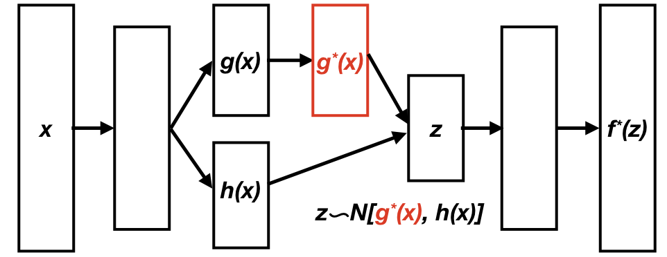
Figure 1: Illustration of network architecture of projection-VAE. It only takes a simple linear projection (red) on the canonical VAE, but ensures the variational distribution has marginal $\mathrm{Cov}(z_{i,k},z_{i,k^{\prime}})=0$ exactly for $k\neq k^{\prime}$, benefiting disentanglement in $f^{*}(z)$ via Stein’s covariance identity.

2.3 Guarantee of Maximal Disentanglement

We now justify why exactly zero correlation is vital for maximal amount of disentanglement.

In order to do so, we need to first formalize the idea of “disentanglement”, by rephrasing maximal disentanglement as “zero entanglement” — specifically, one latent sub-coordinate uniquely controlling one observed facet, is equivalent to the other observed facets not depending on this sub-coordinate. Denoting latent variable as a random vector $\vec{Z}=(Z_{1},\ldots,Z_{d})$, we consider another vector by fixing the $k$th sub-coordinate to constant $c_{k}$

$$\vec{Z}^{\setminus k}:=(Z_{1},\ldots,Z_{k-1},c_{k},Z_{k+1},\ldots,Z_{d}),$$

we can now quantify the dependence via the cross-covariance between $Z_{k}$ and $f^{*}(\vec{Z}^{\setminus k})$.

$$\text{Cross-Cov}[Z_{k},f^{*}(\vec{Z}^{\setminus k})]=\mathbb{E}[Z_{k}-\mathbb{E}Z_{k}][f^{*}(\vec{Z}^{\setminus k})-\mathbb{E}f^{*}(\vec{Z}^{\setminus k})].$$ (3)

Therefore, the closer (3) is to zero, the larger the disentanglement is.

Despite the complexity of the decoder $f^{*}$, we can analytically compute the cross-covariance using Stein’s covariance identity (Stein 1981). We first start with the Gaussian assumption, and quantifiy the mathematical source of entanglement; then we show removing latent correlation leads to zero entanglement, which can be extended to a broad class of continuous distributions.

Theorem 1 (Entanglement under Gaussian encoder).

Let $\vec{Z}=(Z_{1},\dots,Z_{d})^{\prime}$ be a Gaussian random vector. Suppose $f^{*}$ is a neural network such that $\partial f^{*}/\partial z_{k}$ is continuous almost everywhere and $\mathbb{E}|\partial f_{q}^{*}(\vec{Z})/\partial z_{k}|<\infty$ for $q=1,\ldots,p$, then

$$\textup{Cross-Cov}[Z_{k},f^{*}_{q}(\vec{Z}^{\setminus k})]=\sum_{l=1:l\neq k}^{d}\mathrm{Cov}(Z_{k},Z_{l})\mathbb{E}[\frac{\partial f^{*}_{q}(\vec{Z}^{\setminus k})}{\partial Z_{l}}].$$ (4)

Proof.

The proof is a minor extension based on Lemma 1 from Liu (1994), consider $\vec{Z}=\mu+L\vec{Y}$ with $\vec{Y}\sim\text{No}[0,I]$, $LL^{\prime}=\Sigma_{z}$. Using Stein’s lemma,

$$\mathrm{Cov}[Y_{l},g_{1}(\vec{Y})] =\mathbb{E}[\frac{\partial g_{1}(\vec{Y})}{\partial y_{l}}].$$

for $l=1,\ldots,d$ and almost everywhere differentiable function $g_{1}:\mathbb{R}^{p}\to\mathbb{R}$ such that the right hand side is finite. Taking $g_{1}(\vec{Y})=g_{2}[(\mu+L\vec{Y})]$, we have the $d\times 1$ covariance matrix $\mathrm{Cov}[\vec{Z},g_{2}(\vec{Z})]=\Sigma_{z}\nabla g_{2}(\vec{Z})$. Using $g_{2}(\vec{Z})=f^{*}_{q}(\vec{Z}^{\setminus k})$, we have $\partial g_{2}/\partial z_{k}=0$; calculating the matrix product yields the result. ∎

Remark.

the linear form of (4) shows an intuitive decomposition of entanglement: each latent $Z_{l}$ has some influence on the decoder output (quantified as the partial derivative), and the latent covariance acts as the weight coefficient to pass the influence from $Z_{l}$ and intertwine with $Z_{k}$. Clearly, zero covariances among $Z_{k}$’s completely remove the cross-covariance.

Corollary 1.

When the condition in Theorem 1 is satisfied and $\textup{Cov}(Z_{k},Z_{l})=0$ for any $k\neq l$, then $\textup{Cross-Cov}[Z_{k},f^{*}_{q}(\vec{Z}^{\setminus k})]=0$ for all $k=1,\ldots,d$ and $q=1,\ldots,p$.

Thus far, we use the Gaussian assumption on $\vec{Z}$ to illustrate the source of entanglement. One may argue the marginal of $\vec{Z}$ could deviate from Gaussian-ness — indeed, when including the randomness of its mean, we can expect potential longer tail than Gaussian. Therefore, we now relax this to general elliptical distribution — a large distribution class including Laplace, $t$-distribution, etc.

Theorem 2 (Maximal disentanglement under uncorrelated elliptical encoder).

Let $\vec{Z}=(Z_{1},\dots,Z_{d})^{\prime}$ be a continuous random vector from an elliptical distribution with density $h(Z)\propto\mathcal{K}(\vec{Z}^{\prime}\Omega\vec{Z})$ with $\Omega$ positive definite matrix, mean $\mathbb{E}Z_{k}=\mu_{k}$ and variance $\mathrm{Cov}(Z_{k})=\sigma^{2}_{k}<\infty$ for each element. Suppose $f^{*}$ is a neural network such that $\partial f^{*}/\partial z_{k}$ is continuous almost everywhere. If $\mathrm{Cov}(Z_{k},Z_{k^{\prime}})=0$ for $k\neq k^{\prime}$, then $\textup{Cross-Cov}[Z_{k},f^{*}_{q}(\vec{Z}^{\setminus k})]=0$ for all $k=1,\ldots,d$ and $q=1,\ldots,p$.

Proof.

Consider univariate $Y_{k}$ with density $h$, mean $0$ and variance $1$, Goldstein & Reinert (1997) showed that there always exists another random variable $W_{k}$ with density

$$h(w_{k})=\int_{w_{k}}^{\infty}th(t)dt,$$

which is often referred to as the “$Y_{k}$-zero biased” distribution. It has the property:

$$\mathbb{E}_{Y_{k}}Y_{k}g_{1}(Y_{k})=\mathbb{E}_{W_{k}}[\frac{\partial g_{1}(W_{k})}{\partial w_{k}}],$$

which holds for any almost everywhere differentiable $g_{1}:\mathbb{R}\to\mathbb{R}$, such that the right hand side is finite. Naturally, this holds for $g_{1}(Y_{k})=g_{1}(Y_{k};\vec{y}^{\setminus k})$ with any parameter $\vec{y}^{\setminus k}$. Consider

$$g_{1}(Y_{k};\vec{y}^{\setminus k})=f^{*}_{q}(\sigma_{1}y_{1}+\mu_{1},\ldots,c_{k},\ldots,\sigma_{d}y_{d}+\mu_{d})$$ (5)

hence ${\partial g_{1}(W_{k})}/{\partial w_{k}}=0$ almost everywhere. Denoting $m_{k\mid(k)}=\mathbb{E}(Y_{k}\mid\vec{Y}^{\setminus k})$,

$$\mathbb{E}_{\vec{Y}}Y_{k}g_{1}(Y_{k};\vec{Y}\setminus Y_{k}) =\int\int[y_{k}-m_{k\mid(k)}+m_{k\mid(k)}]g_{1}(y_{k};\vec{y}^{\setminus k})h(y_{k}\mid\vec{y}^{\setminus k})h(\vec{y}^{\setminus k})\textup{d}y_{k}\textup{d}\vec{y}^{\setminus k}$$

$$=\int\mathbb{E}_{W_{k}\mid\vec{Y}^{\setminus k}}[\frac{\partial g_{1}(W_{k};\vec{y}^{\setminus k})}{\partial w_{k}}]h(\vec{y}^{\setminus k})\textup{d}y_{k}\textup{d}\vec{y}^{\setminus k}$$

$$+\int\int m_{k\mid(k)}g_{1}(y_{k};\vec{y}^{\setminus k})h(y_{k}\mid\vec{y}^{\setminus k})h(\vec{y}^{\setminus k})\textup{d}y_{k}\textup{d}\vec{y}^{\setminus k}.$$

The first term on the right hand side is zero as proved above. The second term is also zero due to $m_{k\mid(k)}=m_{k}=0$, as the property of elliptical distribution (Owen & Rabinovitch 1983).

Notice the above left hand side is equal to

$$\mathbb{E}_{\vec{Y}}[Y_{k}g_{1}(Y_{k};\vec{Y}\setminus Y_{k})]-(\mathbb{E}_{Y_{k}}Y_{k})[\mathbb{E}_{\vec{Y}}g_{1}(Y_{k};\vec{Y}\setminus Y_{k})]=\mathrm{Cov}[Y_{k},g_{1}(Y_{k};\vec{Y}\setminus Y_{k})]$$

taking $Z_{k}=\sigma_{k}Y_{k}+\mu_{k}$ and (5), we have $\mathrm{Cov}[Z_{k},f^{*}_{q}(\vec{Z}^{\setminus k})]=0$. ∎

Remark.

As we have generalized beyond Gaussian class, this means we do not need independence among $\vec{Z}$ to induce disentanglement.

2.4 Preserving Information

Intuitively, rotation and scaling do not change the amount of information stored in the encoder mean $\{g(x_{1}),\ldots,g(x_{n})\}$. One can quantify the ‘expressiveness’ via entropy, i.e. the information diversity. We now show this is preserved under bijective transform.

Theorem 3 (Invariance of Entropy under Bijective Function).

For discrete random variable $X$ and an bijective function $m$,

$$\mathrm{H}\big{\{}m[g(X)]\big{\}}=\mathrm{H}\big{[}g(X)\big{]}.$$

Proof.

Consider the joint entropy, decomposed as the sum of marginal and conditional entropies

$$\mathrm{H}\{m[g(X)],g(X)\}=\mathrm{H}[g(X)]+\mathrm{H}\{m[g(X)]|g(X)\}=\mathrm{H}\{m[g(X)]\}+\mathrm{H}\{g(X)|m[g(X)]\}.$$

Since $m$ is a deterministic function, $\mathrm{H}\{m[g(X)]|g(X)\}=0$ and thus $\mathrm{H}[g(X)]=\mathrm{H}\{m[g(X)]\}+\mathrm{H}\{g(X)|m[g(X)]\},$ so $\mathrm{H}[g(X)]\geq\mathrm{H}\big{\{}m[g(X)]\big{\}}.$

Since $m$ is bijective, then there exits an inverse function $m^{-1}$ such that $g(X)=m^{-1}\{m[g(X)]\}$, then applying the previous result yields $\mathrm{H}[g(X)]\leq\mathrm{H}\big{\{}m[g(X)]\big{\}}$. Combining two pieces yields the result. ∎

Remark.

In our case, $m[g(x_{i})]=L^{\prime}[g(x_{i})-\mu_{g}]+\mu_{g}$, where $L$ is a $d\times d$ invertible matrix; hence this is an bijective function.

Since zero correlation constraint is directly accommodated when projecting $g$ into $g^{*}$, all the previous layers in $g$ remain fully flexible. This is fundamentally different from correlation-based regularization that applies on the whole encoder; the practical difference in performance will also be illustrated in the data experiments.

3 Data Experiments

We now use common benchmark datasets to demonstrate good performance of Proj-VAE — to clarify, we do not claim always superior performance than competitors — as the evaluation of disentanglement can be quite subjective. Rather, we want to emphasize on the tuning-free property of Proj-VAE, with good reconstruction accuracy. This makes it an appealing tool for almost automatic dimension reduction.

3.1 Reconstruction Accuracy

To illustrate that projection has almost no impact on expressiveness, we use the images of Frey Face. Since this is a small dataset with $n=1,900$, it is easy to train most models to their minimal loss — this is important for a fair comparison on the reconstruction accuracy. For simplicity, we run four models with $d=3$ latent dimension, and only one hidden layer in encoder and decoder with $256$ units.

Figure 2 shows that the reconstructions from Proj-VAE are almost indistinguishable to the canonical VAE. On the other hand, the correlation-based regularization with penalty $\gamma\|\Sigma_{g}-I_{d}\|_{1}$ and $\gamma=100$, severely impacts the reconstruction. This demonstrates the sharp distinction between projection and regularization.

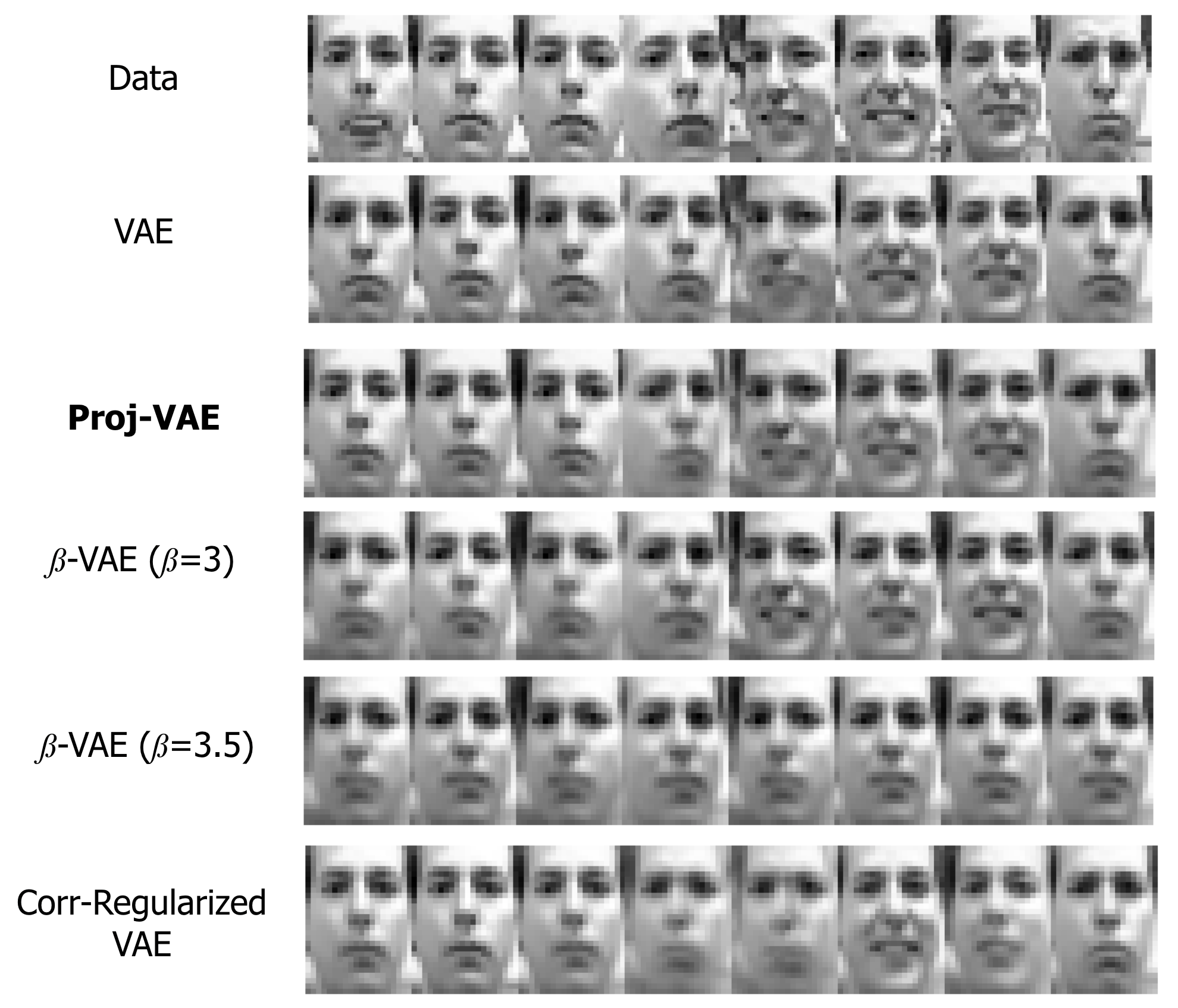
Figure 2: Comparison of the reconstructed images to the original data (first row), using canonical VAE, Proj-VAE, $\beta$-VAE and Correlation-regularized VAE. Proj-VAE shows almost identical reconstruction to the canonical VAE (with average binary cross-entropy errors $346.2$ and $344.0$, respectively); correlation-based regularization (last row) severely impacts the expressiveness (with error $350.1$); $\beta$-VAE requires a careful tuning as slightly increased $\beta$ can result in loss of feature (mouth).

To show the effectiveness of removing correlation via projection, Figure 3 plots the correlation matrices $\text{Corr}[g^{*}_{k}(x_{i}),g^{*}_{k^{\prime}}(x_{i})]$ on the scale of $\log_{10}$ of absolute value. The results are compared against the $\text{Corr}[g_{k}(x_{i}),g_{k^{\prime}}(x_{i})]$ in correlation-regularized VAE. The projection achieves precision around $10^{-7}$, which is the float precision in typical GPU-based program; whereas penalty with $\gamma=100$ on the correlation can only yield $10^{-2}$. Further increasing $\gamma$ in regularization is not practical as it incurs more reconstruction error.

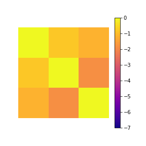
(a) Correlation-based Regularization

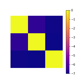
(b) Projection

Figure 3: Comparing the numeric values of correlation matrices ( on the scale of $\log_{10}|\text{Corr|}$) in the Gaussian means for latent $z$.

3.2 Disentanglement Performance

To demonstrate the disentanglement performance in a relatively large dataset, we use the chairs dataset (Aubry et al. 2014), which contains $n=86,366$ images of chair CAD models. We use $d=16$ and the same architecture of convolutional network as described in Higgins et al. (2017).

We select three factors and present them in Figure 4. In Proj-VAE, the azimuth rotation and backrest height of the chairs are clearly separated (panel a). In comparison, the canonical VAE (panel b) and $\beta$-VAE (panel c, $\beta=5$) have those two factors mixed together, although we expect $\beta$-VAE can disentangle them with larger $\beta$.

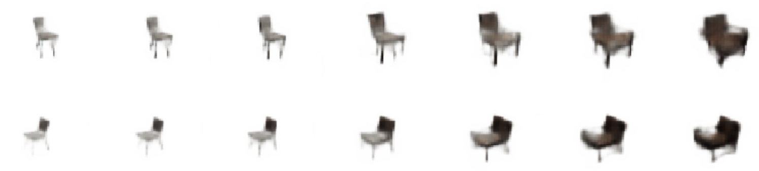
i. Scale

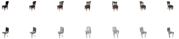
ii. Rotation

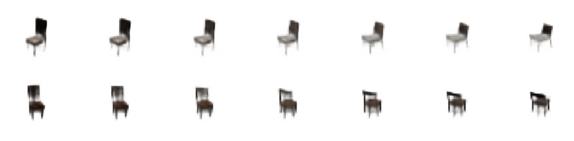
iii. Backrest height

(a) Disentangled representation learned by Proj-VAE.

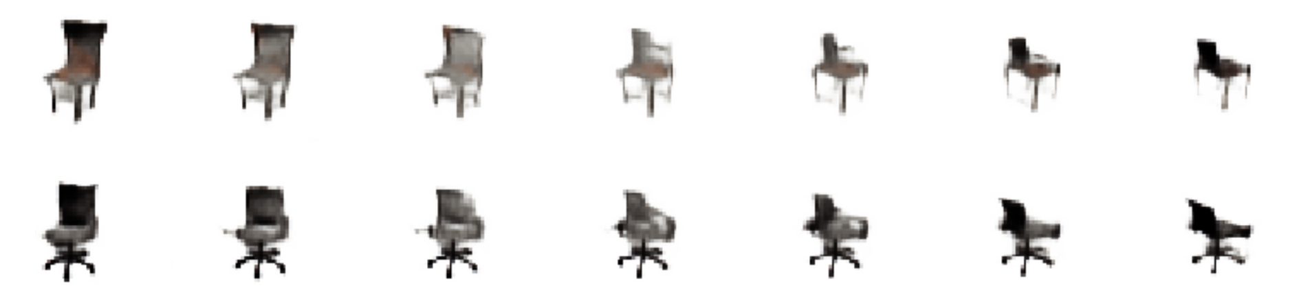
Rotation and Backrest height

(b) Two factors are entangled in the canonical VAE.

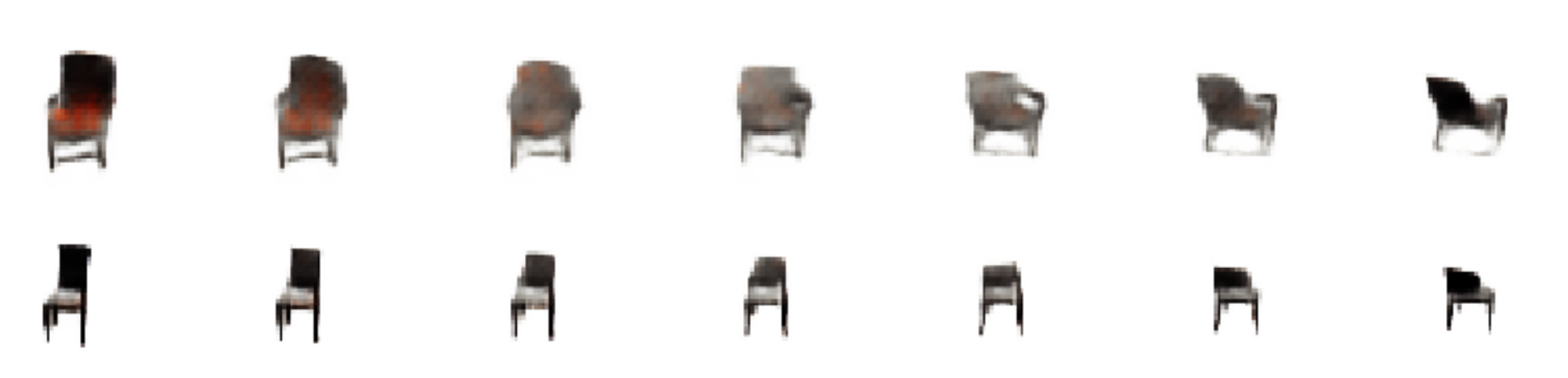
Rotation and Backrest height

(c) Two factors are still entangled in the $\beta$-VAE when $\beta=5$.

Figure 4: Generated chair images using different VAEs: each row of the data are simulated with one $z_{.,k}$ traversing from $-3$ to $3$ (the approximate learned range), while keeping the other factors fixed. Proj-VAE learns disentangled representation of rotation and backrest height, compared to canonical VAE (panel b) and $\beta$-VAE with $\beta=5$.

We also apply Proj-VAE on a large data CelebA (Liu et al. 2015), which includes $n=202,599$ celebrity images over 3 color channels. We choose $d=32$ as selected by $\beta$-VAE (Higgins et al. 2017) and FactorVAE (Kim & Mnih 2018). Our approach learns all the factors previously reported, such as skin color, image saturation, age, gender, rotation, emotion and fringe (discovered in $\beta$-VAE with $\beta=250$ and FactorVAE with $\gamma=6.4$). Interestingly, It also discovers several new factors, such as the presence of sunglasses, background brightness and color tint. Again, existing approaches can find the same factors under appropriate tuning — for example, sunglasses factor can be recovered in $\beta$-VAE with much smaller $\beta=10$ (this seems coherent with the fact that those variations are on a finer scale); our advantage is that there is no tuning required, hence it takes only one time of training.

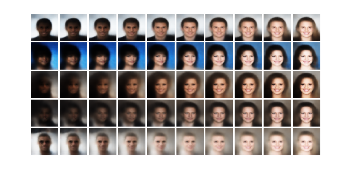
(a) Skin Color

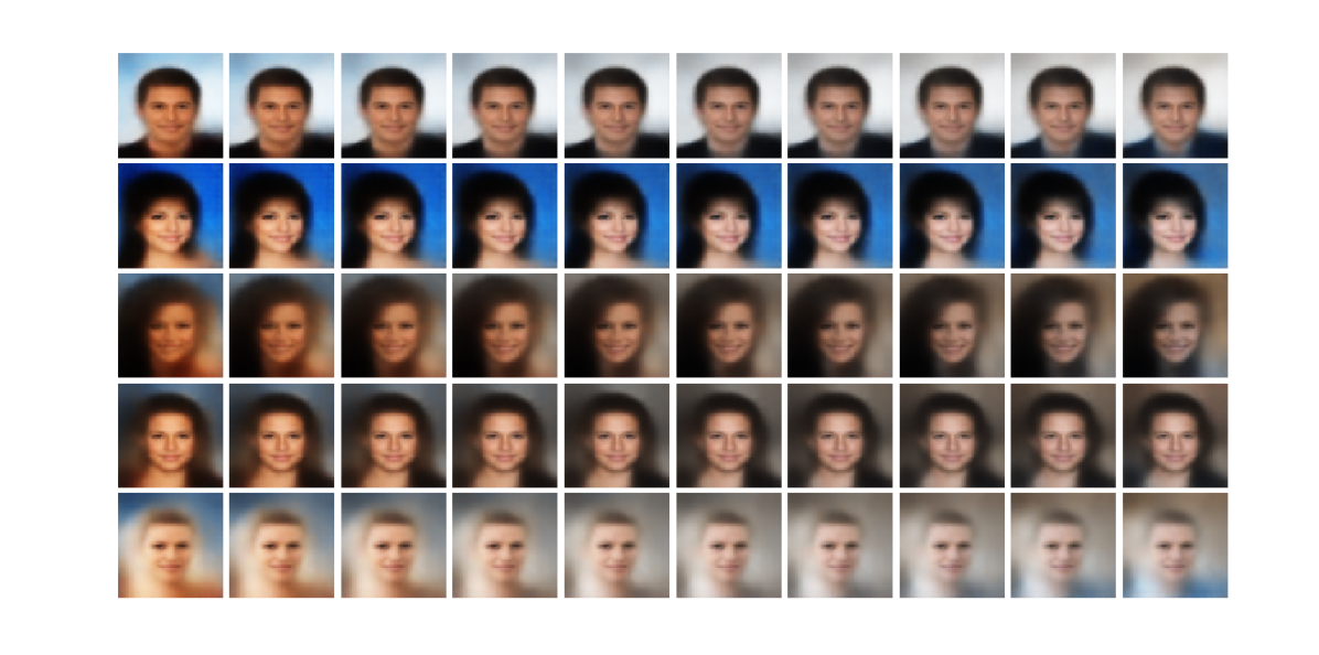
(b) Image Saturation

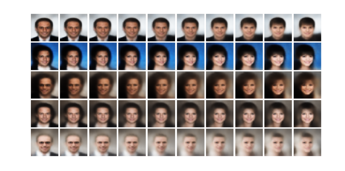
(c) Gender

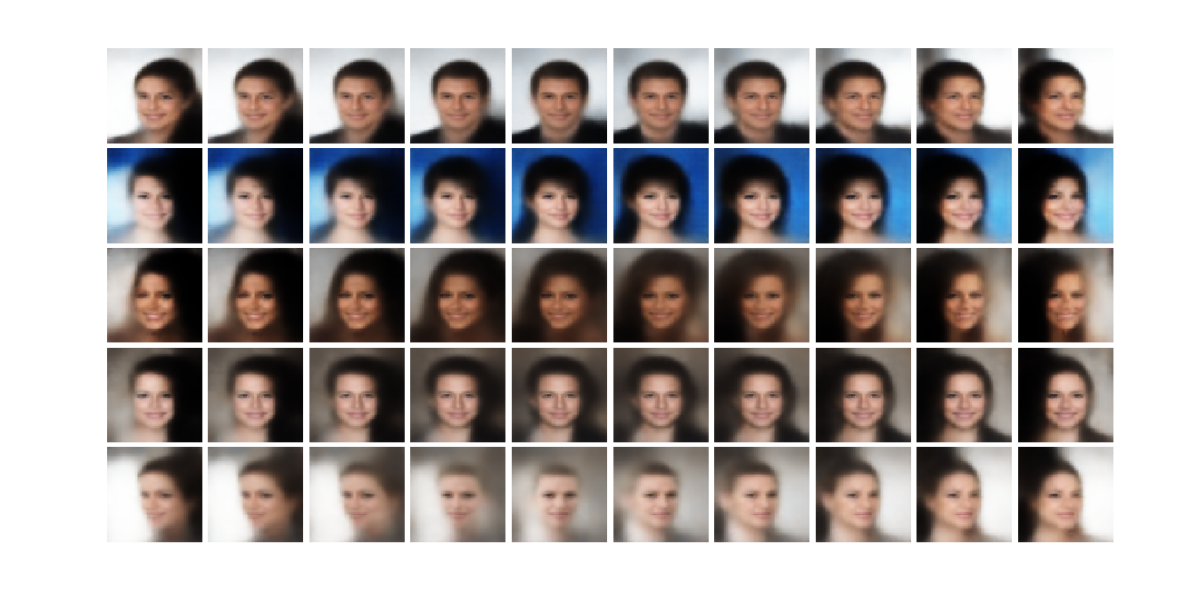
(d) Rotation

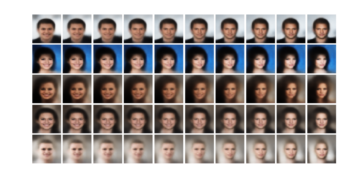
(e) Emotion(Smile-Neutral)

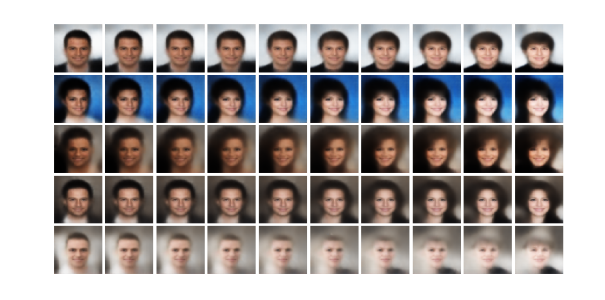
(f) Hair(Fringe)

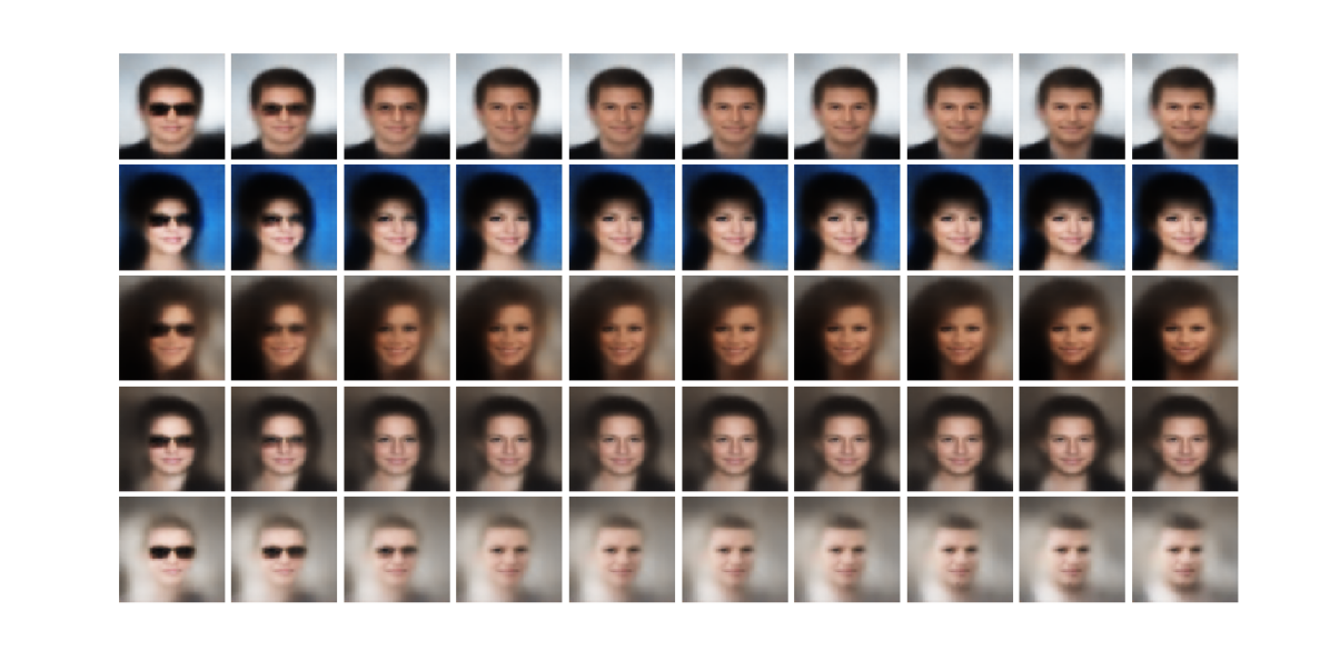
(g) Sunglasses

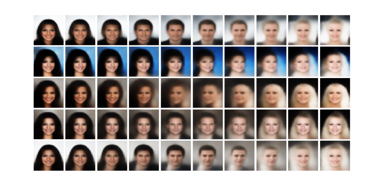
(h) Hair Color(Black-White)

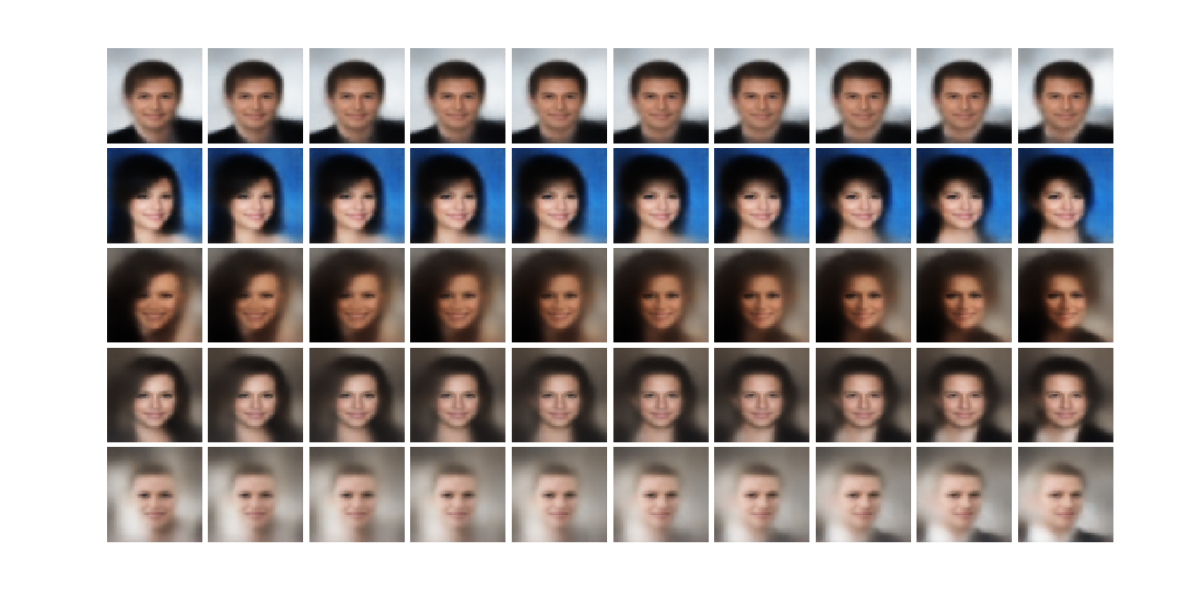
(i) Hair (Side Part)

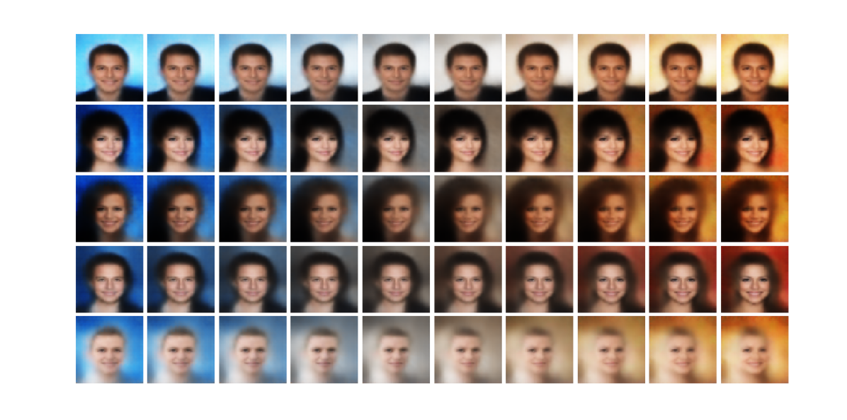
(j) Background Tint (Red-Blue)

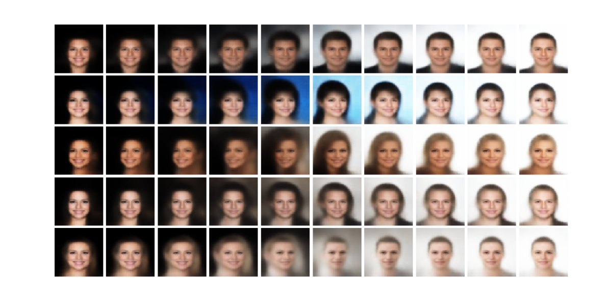
(k) Background Brightness

Figure 5: Disentangled factors found by Proj-VAE in CelebA dataset.

4 Discussion

We demonstrate a simple projection in Proj-VAE can lead to surprisingly good disentangling performance, bypassing the need of heuristic tuning. This idea has an interesting support from the classic statistical theory. For concise exposition, we leave out several interesting extensions — for example, what is the ideal number of latent dimensions $d$? This problem has recently been considered by Kim et al. (2019) via a prior shrinkage on $d$. In this article, we choose a conservatively small $d$, such that most of the factors can be interpretable. On the other hand, we did experiment with much larger $d$ (e.g. $d=5$ in Frey Face data, $d=32$ in chairs data) and the model seems to further capture variations in a smaller subset of data. To accommodate this, it appears intuitive to consider a mixture of Gaussians with an alternative projection scheme to remove correlation, for example, the Factor-VAE(Kim & Mnih 2018) takes the marginal distribution $q(z)$ into account which involves mixtures with a large number of components rather than the Gaussian, leading the model to learn more informative disentangled latent representations; Furthermore, it remains to see if the disentanglement theory holds for mixture, and how to derive a solution as simple as Gaussian Proj-VAE.

References

- (1)
- Achille & Soatto (2018) Achille, A. & Soatto, S. (2018), ‘Emergence of invariance and disentanglement in deep representations’, The Journal of Machine Learning Research 19(1), 1947–1980.
- Aubry et al. (2014) Aubry, M., Maturana, D., Efros, A. A., Russell, B. C. & Sivic, J. (2014), Seeing 3d chairs: exemplar part-based 2d-3d alignment using a large dataset of cad models, in ‘Proceedings of the IEEE conference on Computer Vision and Pattern Recognition’, pp. 3762–3769.
- Chen et al. (2016) Chen, X., Duan, Y., Houthooft, R., Schulman, J., Sutskever, I. & Abbeel, P. (2016), InfoGAN: Interpretable representation learning by information maximizing generative adversarial nets, in ‘Advances in Neural Information Processing Systems’, pp. 2172–2180.
- Cheung et al. (2014) Cheung, B., Livezey, J. A., Bansal, A. K. & Olshausen, B. A. (2014), ‘Discovering hidden factors of variation in deep networks’, arXiv preprint arXiv:1412.6583 .
- Cogswell et al. (2015) Cogswell, M., Ahmed, F., Girshick, R., Zitnick, L. & Batra, D. (2015), ‘Reducing overfitting in deep networks by decorrelating representations’, arXiv preprint arXiv:1511.06068 .
- Goldstein & Reinert (1997) Goldstein, L. & Reinert, G. (1997), ‘Stein’s method and the zero bias transformation with application to simple random sampling’, The Annals of Applied Probability 7(4), 935–952.
- Götze & Tikhomirov (2010) Götze, F. & Tikhomirov, A. N. (2010), ‘The rate of convergence of spectra of sample covariance matrices’, Theory of Probability & Its Applications 54(1), 129–140.
- Higgins et al. (2017) Higgins, I., Matthey, L., Pal, A., Burgess, C., Glorot, X., Botvinick, M., Mohamed, S. & Lerchner, A. (2017), -VAE: learning basic visual concepts with a constrained variational framework, in ‘International Conference on Learning Representations’, Vol. 3.
- Hjelm et al. (2018) Hjelm, R. D., Fedorov, A., Lavoie-Marchildon, S., Grewal, K., Trischler, A. & Bengio, Y. (2018), ‘Learning deep representations by mutual information estimation and maximization’, arXiv preprint arXiv:1808.06670 .
- Kim & Mnih (2018) Kim, H. & Mnih, A. (2018), ‘Disentangling by factorising’, arXiv preprint arXiv:1802.05983 .
- Kim et al. (2019) Kim, M., Wang, Y., Sahu, P. & Pavlovic, V. (2019), ‘Relevance factor VAE: Learning and identifying disentangled factors’, arXiv preprint arXiv:1902.01568 .
- Kingma & Welling (2013) Kingma, D. P. & Welling, M. (2013), ‘Auto-encoding variational Bayes’, arXiv preprint arXiv:1312.6114 .
- Kumar et al. (2017) Kumar, A., Sattigeri, P. & Balakrishnan, A. (2017), ‘Variational inference of disentangled latent concepts from unlabeled observations’, arXiv preprint arXiv:1711.00848 .
- Liu (1994) Liu, J. S. (1994), ‘Siegel’s formula via Stein’s identities’, Statistics & Probability Letters 21(3), 247–251.
- Liu et al. (2015) Liu, Z., Luo, P., Wang, X. & Tang, X. (2015), Deep learning face attributes in the wild, in ‘Proceedings of the IEEE International Conference on Computer Vision’, pp. 3730–3738.
- Owen & Rabinovitch (1983) Owen, J. & Rabinovitch, R. (1983), ‘On the class of elliptical distributions and their applications to the theory of portfolio choice’, The Journal of Finance 38(3), 745–752.
- Stein (1981) Stein, C. M. (1981), ‘Estimation of the mean of a multivariate normal distribution’, Annals of Statistics pp. 1135–1151.