GASP, a generalized framework for agglomerative clustering of signed graphs and its application to Instance Segmentation

Abstract

We propose a theoretical framework that generalizes simple and fast algorithms for hierarchical agglomerative clustering to weighted graphs with both attractive and repulsive interactions between the nodes. This framework defines GASP, a Generalized Algorithm for Signed graph Partitioning, and allows us to explore many combinations of different linkage criteria and cannot-link constraints. We prove the equivalence of existing clustering methods to some of those combinations and introduce new algorithms for combinations that have not been studied before. We study both theoretical and empirical properties of these combinations and prove that some of these define an ultrametric on the graph. We conduct a systematic comparison of various instantiations of GASP on a large variety of both synthetic and existing signed clustering problems, in terms of accuracy but also efficiency and robustness to noise. Lastly, we show that some of the algorithms included in our framework, when combined with the predictions from a CNN model, result in a simple bottom-up instance segmentation pipeline. Going all the way from pixels to final segments with a simple procedure, we achieve state-of-the-art accuracy on the CREMI 2016 EM segmentation benchmark without requiring domain-specific superpixels.

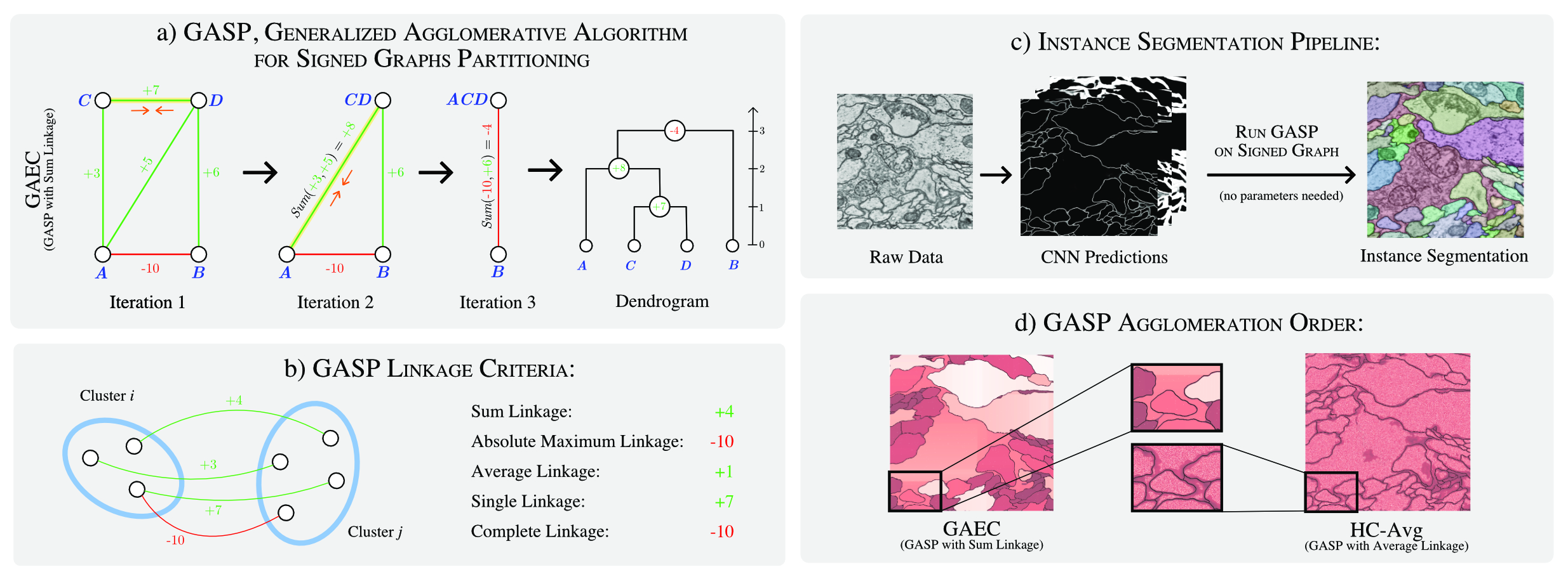
Figure 1: (a) Some iterations of GASP on a graph with attractive (green) and repulsive (red) interactions. At each iteration, the yellow edge with highest weight is contracted (example with sum linkage criterion is shown). (b) Linkage criteria used in this paper demonstrated on two small clusters (see definitions in Table 1 below). (c) Application of GASP to instance segmentation: we show raw data from the CREMI neuron-segmentation challenge and some predictions of our CNN model, where white pixels represent boundary evidence. (d) Seemingly similar linkage criteria can result in very different clustering dynamics, as shown in this example: color coded sequence of merges from early (white) via late (brown) to never (black).

GASP	Sum Linkage	Absolute Maximum Linkage	Average Linkage	Single Linkage	Complete Linkage
	$\displaystyle\sum_{e\in E_{ij}}w_{e}$	$\displaystyle w_{e}$ with $\displaystyle e=\operatorname*{arg\,max}_{t\in E_{ij}}|w_{t}|$	$\displaystyle\sum_{e\in E_{ij}}w_{e}\bigg{/}\big{|}E_{ij}\big{|}$	$\displaystyle\max_{e\in E_{ij}}w_{e}$	$\displaystyle\min_{e\in E_{ij}}w_{e}$
Unsigned graphs	-	HC-Single	HC-Avg	HC-Single	HC-Complete
Signed graphs	GAEC [39]	Mutex Watershed [75]	HC-Avg	HC-Single	HC-Complete
Signed graphs + cannot-link constraints	HCC-Sum	Mutex Watershed [75]	HCC-Avg	HCC-Single	HC-Complete

Table 1: Conceptual contribution: Properties of clustering algorithms included in the proposed GASP framework, given a linkage criterion, a type of graph (signed or unsigned) and the optional use of cannot-link constraints. New constrained hierarchical clustering algorithms (HCC) proposed in this paper are highlighted in yellow. For algorithms typeset in bold font we prove that they define an ultrametric on the graph (Eq. 3). For algorithms in the green box we show that they are weight-shift invariant (Prop. 3.2). Notation: $E_{ij}$ denotes the set of edges connecting two clusters $S_{i},S_{j}\subseteq V$.

1 Introduction

In computer vision, the partitioning of weighted graphs has been successfully applied to tasks as diverse as image segmentation, object tracking and pose estimation. Most graph clustering methods work with positive edge weights only, which can be interpreted as similarities or distances between the nodes. These methods require users to specify the desired numbers of clusters (as in spectral clustering) or a termination criterion (e.g. in iterated normalized cuts) or even to add a seed for each object (e.g. seeded watershed or random walker).

Other graph clustering methods work with so-called signed graphs, which feature both positive and negative edge weights corresponding to attraction and repulsion between nodes. The advantage of signed graphs over unsigned graphs is that balancing attraction and repulsion allows us to obtain a clustering without defining additional parameters. A canonical formulation of the signed graph partitioning problem is the multicut or correlation clustering problem [35, 15]. This problem is NP-hard, though many approximate solvers have been proposed [47, 62, 8, 77] together with greedy agglomerative clustering algorithms [39, 51, 75, 36]. Agglomerative clustering algorithms for signed graphs have clear advantages: they are parameter-free and efficient. Despite the fact that a variety of these algorithms exist, no overarching study has so far been conducted to compare their robustness and efficiency or to provide guidelines for matching an algorithm to the partitioning problem at hand.

Our first contribution is a simple theoretical framework that generalizes over agglomerative algorithms for signed graphs by linking them to hierarchical clustering (HC) on unsigned graphs (Section 3.2). This framework defines an underlying basic algorithm and allows us to explore its combinations with different linkage criteria and cannot-link constraints (see Fig. 1a, 1b, and Table 1). As second contribution, in Section 3.3, we formally prove that some of the combinations correspond to existing clustering algorithms, and introduce new algorithms for combinations which have not been explored before. By analyzing their theoretical properties, we also show that some of them define an ultrametric on the graph (see Table 1).

Third, we evaluate the algorithms on a large variety of both existing and synthetically generated signed graph clustering problems (Section 4). Fourth and finally, we also test the algorithms on instance segmentation – a computer vision task consisting of assigning each pixel of an image to an object instance – by partitioning graphs whose edge weights are estimated by a CNN (see Fig. 1c and Section 4.2). Our experiments show that the choice of linkage criterion markedly influences how clusters are grown by the agglomerative algorithms (Fig. 1d), making some linkage methods more suited for certain types of clustering problems. We benchmark the clustering algorithms by focusing on their efficiency, robustness and tendency to over- or under-cluster. On instance segmentation, we show that the agglomerative algorithms outperform recently proposed spectral clustering methods, and that average-linkage based agglomerative algorithms achieve state of the art results on the CREMI 2016 challenge for neuron segmentation of 3D electron microscopy image volumes of brain tissue.

2 Related work

Proposal-free instance segmentation methods adopt a bottom-up approach by directly grouping pixels into instances. In the last years, there has been a growing interest in such methods that do not involve object detection because, in certain types of data, object instances cannot be approximated by bounding boxes [41, 5]. Some use metric learning to predict high-dimensional associative pixel embeddings that map pixels of the same instance close to each other [49, 23, 60, 21] and then retrieve final instances by applying a clustering algorithm [44]. Other recent methods let the model predict the relative coordinates of the instance center [59, 13] or, given a pixel $(x,y)$, they train a model to generate the mask of the instance located at $(x,y)$ [70].

Edge detection also experienced recent progress thanks to deep learning, both on natural images [29, 55, 76, 43] and biological data [50, 69, 57, 18]. In neuron segmentation for connectomics, a field of neuroscience we also address in our experiments, boundaries are converted to final instances with subsequent postprocessing and superpixel-merging: some use a combinatorial framework [10], others use loopy graphs [37, 45] or trees [57, 54, 52, 26, 72] to represent the region merging hierarchy. Flood-filling networks [32] and MaskExtend [57] used a CNN to iteratively grow one region/neuron at the time. A structured learning approach was also proposed in [28, 71].

Agglomerative graph clustering has often been applied to instance segmentation [3, 66, 53, 68] because of its efficiency as compared to other divisive approaches like graph cuts. Novel termination criteria and merging strategies have often been proposed: the agglomeration in [56] deploys fixed sets of merge constraints; the popular graph-based method [24] stops the agglomeration when the merge costs exceed a measure of quality for the current clusters. The optimization approach in [40] performs greedy merge decisions that minimize a certain energy, while other pipelines use classical linkage criteria, e.g. average linkage [55, 50], median [28] or a linkage learned by a random forest classifier [61, 42].

Clustering of signed graphs has the goal of partitioning a graph with both attractive and repulsive cues. Finding an optimally balanced partitioning has a long history in combinatorial optimization [30, 31, 16]. NP-hardness of the correlation clustering problem was shown in [7], while the connection with graph multicuts was made by [22]. Modern integer linear programming solvers can tackle problems of considerable size [2], but accurate approximations [62, 8, 77], greedy agglomerative algorithms [51, 74, 39, 36] and persistence criteria [48, 47] have been proposed for even larger graphs. Another line of research is given by spectral clustering methods that, on the other hand, require the user to specify the number of clusters in advance. Recently, some of these methods have been generalized to graphs with signed weights [19, 14, 46], whereas others let the user specify must-link and cannot-link constraints between clusters [65, 73, 20].

This work reformulates the clustering algorithms of [51, 75, 39] in a generalized framework and adopts ideas from the proposal-free instance segmentation methods [55, 75, 50] to predict edge weights of a graph.

3 Generalized framework for agglomerative clustering of signed graphs

3.1 Notation

Graph formalism – We consider an undirected simple edge-weighted graph $\mathcal{G}(V,E,w^{+},w^{-})$ with both attractive and repulsive edge attributes. The weight function $w^{+}:E\rightarrow\mathbb{R}^{+}$ associates to every edge a positive scalar attribute $w_{e}^{+}\in\mathbb{R}^{+}$ representing a merge affinity or a similarity measure. On the other hand, $w^{-}:E\rightarrow\mathbb{R}^{+}$ associates to each edge a split tendency $w_{e}^{-}\in\mathbb{R}^{+}$. Graphs of the type $\mathcal{G}(V,E,w^{+},w^{-})$ are often defined as signed graphs $\mathcal{G}(V,E,w)$, featuring positive and negative edge weights $w_{e}\in\mathbb{R}$. Following the theoretical considerations in [48], we define signed weights as ${w_{e}=w_{e}^{+}-w_{e}^{-}}$.

Multicut objective – We call the set $\Pi=\{S_{1},\ldots,S_{K}\}$ a clustering or partitioning if $V=\cup_{S\in\Pi}S$, $\,S\cap S^{\prime}=\emptyset$ for different clusters $S,S^{\prime}$ and every cluster $S\in\Pi$ induces a connected subgraph of $\mathcal{G}$. For any clustering $\Pi$ of $\mathcal{G}$, we denote as $E^{0}_{\Pi}=\{e_{uv}\in E\,|\,\exists S\in\Pi:u,v\in S\}$ the set of edges linking nodes in the same cluster. Its complementary set $E_{\Pi}^{1}=E\setminus E^{0}_{\Pi}$ of edges linking nodes belonging to distinct clusters, is known as the multicut of $\mathcal{G}$ associated to clustering $\Pi$. The instance of the NP-hard minimum cost multicut problem w.r.t. $\mathcal{G}(V,E,w_{e})$ is the task of finding a clustering that optimally balances the attraction and repulsion in the graph and is given by the following binary integer program:

$$\min_{\Pi}\sum_{e\in E}w_{e}x_{e}^{\Pi},\qquad\text{where}\quad x^{\Pi}_{e}=\begin{cases}1&\text{if }e\in E^{1}_{\Pi}\\ 0&\text{otherwise}.\end{cases}$$ (1)

Linkage criteria and hierarchical trees – Let the interaction $\mathcal{W}(S\cup S^{\prime})\in\mathbb{R}$ between two clusters $S,S^{\prime}$ be defined as a function, named linkage criterion, depending on the weights of all edges connecting clusters $S$ and $S^{\prime}$. The linkage criteria tested in this article are listed and defined in Table 1. A dendrogram $T$ is a rooted binary tree representing the merging order of an agglomerative algorithm, such that the leaves of the tree are in one-to-one correspondence with $V$ and each node of the tree represents a merge between two clusters. Let $T_{\mathrm{R}},T_{\mathrm{L}}\subset T$ denote the subtrees rooted at the two children of the root node in $T$. For any two leaves $u,v\in V$, let $T[u\vee v]$ be the subtree rooted at the least common ancestor $(u\vee v)\in T$ of nodes $u$ and $v$ (furthest from the root), and let leaves$(T[u\vee v])\subseteq V$ be the set of leaves of this subtree. Given an agglomerative algorithm with merging tree $T$, let $h_{T}:V\times V\rightarrow\mathbb{N}$ denote the dendrogram-height of each $(u\vee v)\in T$, which is defined as the iteration number at which nodes $u,v\in V$ were merged by the algorithm (see example in Fig. 1a). We also define $\mathcal{W}{}_{T}(u,v)$ as the signed interaction $\mathcal{W}{}(S\cup S^{\prime})$ between the two clusters $S,S^{\prime}$ that were merged at iteration $h_{T}(u,v)$:

$$\mathcal{W}{}_{T}(u,v)\equiv\mathcal{W}{}\big{(}\text{{leaves}}(T_{\mathrm{R}}[u\vee v])\cup\text{{leaves}}(T_{\mathrm{L}}[u\vee v])\big{)}$$ (2)

3.2 The GASP algorithm

Our main contribution is a generalized agglomerative algorithm for signed graph partitioning (GASP) that generalizes hierarchical clustering (HC) to signed graphs. The framework, defined in the following, encompasses several known and new agglomerative algorithms on display in Table 1, which are differentiated by the linkage criterion employed, similarly to HC.

In Algorithm 1, we provide simplified pseudo-code for the proposed GASP algorithm. GASP implements a bottom-up approach that starts by assigning each node to its own cluster and then iteratively merges pairs of adjacent clusters. The algorithm proceeds in three phases.

In phase one, GASP selects the pair of clusters with the highest absolute interaction $|\mathcal{W}(S\cup S^{\prime})|$, so that the most attractive and the most repulsive pairs are analyzed first. If the interaction is repulsive and the algorithm option addCannotLinkConstraints is True, then the two clusters are constrained so that their members can never merge in subsequent steps of phase one. If the interaction is attractive, then the clusters are merged, provided that they were not previously constrained. After each merge, the interaction between the merged cluster and its neighbors is updated according to one of the linkage criteria $\mathcal{W}(S\cup S^{\prime})$ listed in Table 1. Phase one terminates when all the remaining clusters are either constrained or share repulsive interactions. Note that, on unsigned graphs, in phase one all nodes are merged into a single cluster and GASP is then equivalent to a standard hierarchical clustering algorithm.

Phase two: Now that the clusters have grown in size, the algorithm removes the constraints previously introduced in phase one and merges all the clusters that still share an attractive interaction, merging the most attractive one first. The final clustering $\Pi^{*}$ returned by GASP is found at the end of phase two and it is then composed of clusters sharing only mutual repulsive interactions.

Finally, in phase three, the algorithm keeps merging all clusters until only a single one is left and then returns the hierarchical tree $T^{*}$ representing the full sequence of merging steps. The algorithm was implemented using a standard HC implementation with computational complexity $\mathcal{O}(N^{2}\log N)$ (details left in Appendix A6.1).

Algorithm 1 GASP

Input: Graph $\mathcal{G}(V,E,w^{+},w^{-})$; linkage criterion $\mathcal{W}{}$;

boolean addCannotLinkConstraints

Output: Final clustering $\Pi^{*}$, rooted binary hierarchical tree $T^{*}$

1:Initial clustering: $\Pi=\{\{v_{1}\},\ldots,\{v_{|V|}\}\}$

2:Initialize hierarchical tree $T^{*}$ with leaf nodes $V=\{v_{1},\ldots,v_{|V|}\}$

3:Initialize cluster interactions with $w_{e}=w^{+}_{e}-w^{-}_{e}$, $\forall e\in E$

4:// Phase 1: Merge positive interactions (possibly using constraints)

5:Push incident nodes of every edge $e\in E$ to priority queue (PQ) with priority $|w_{e}|$

6:repeat

7:  Pop $S,S^{\prime}\in\Pi$ with highest interaction $|\mathcal{W}{}(S\cup S^{\prime})|$ from PQ

8:  if [$\mathcal{W}{}(S\cup S^{\prime})>0$] and [$S,S^{\prime}$ not constrained] then

9:    Merge clusters $S$, $S^{\prime}$ and update hierarchical tree $T^{*}$

10:    Update interactions & constraints with neighboring clusters

11:  else if addCannotLinkConstr and [$\mathcal{W}{}(S\cup S^{\prime})\leq 0$] then

12:    Add CannotLink Constraint between $S$ and $S^{\prime}$   

13:until [$PQ$ is empty]

14:// Phase 2: Remove constraints & merge all positive interactions

15:Push signed interactions $\mathcal{W}{}(S\cup S^{\prime})$ to PQ, $\forall S,S^{\prime}\in\Pi$

16:repeat

17:  Pop $S,S^{\prime}\in\Pi$ with highest interaction $\mathcal{W}{}(S\cup S^{\prime})$ from PQ

18:  if [$\mathcal{W}{}(S\cup S^{\prime})>0$] then

19:    Merge clusters $S$, $S^{\prime}$ and update hierarchical tree $T^{*}$

20:    Update interactions with neighboring clusters   

21:until [$\mathcal{W}{}(S\cup S^{\prime})\leq 0$]

22:Save the final clustering $\Pi^{*}\leftarrow\Pi$

23:// Phase 3: Merge negative interactions until one single cluster is left

24:repeat

25:  Pop $S,S^{\prime}\in\Pi$ with highest interaction $\mathcal{W}{}(S\cup S^{\prime})$ from PQ

26:  Merge clusters $S$, $S^{\prime}$ and update hierarchical tree $T^{*}$

27:  Update interactions with neighboring clusters

28:until [Only one cluster is left in $\Pi$]

29:return $\Pi^{*}$, $T^{*}$

3.3 GASP: New and existing algorithms

In this paper we focus on five linkage methods (see columns of Table 1). Many more linkage criteria have been applied to unsigned graphs [61, 24, 28], involving median-based or size-regularized methods, but we decided to focus this paper on those five criteria because they represent the most popular choices.

Sum Linkage

– On signed graphs, the sum of two attractive (or repulsive) interactions is still attractive (repulsive). On the other hand, on unsigned graphs, a strong attractive interaction could be obtained by summing many weak interactions, which depending on the application could be undesirable. This explains why, to our knowledge, an agglomerative algorithm with sum linkage has never been used on unsigned graphs. On signed graphs, such an algorithm was pioneered in [51, 39] and was named Greedy Agglomerative Edge Contraction (GAEC). GAEC always makes the greedy choice that most decreases the multicut objective defined in Eq. 1 each time two clusters with positive interaction are merged. The authors of [51] propose an algorithm named GreedyFixation, which is equivalent to phase one of GASP using cannot-link-constraints and a sum linkage. However, running both phase one and two of GASP with sum linkage (algorithm named HCC-Sum in this paper) performed better than GreedyFixation in our experiments.

AbsMax Linkage

– This linkage method is also specific to signed graphs, since on unsigned graphs it would be equivalent to single linkage. Here, we prove that the Mutex Watershed Algorithm [75] can be seen as an agglomerative algorithm with AbsMax linkage (proofs of the following three propositions are given in Appendix A6.3):

Proposition 3.1.

The GASP Algorithm 1 with AbsMax linkage, with or without cannot link constraints, returns the same final clustering $\Pi^{*}_{\mathrm{AbsMax}}$ also returned by the Mutex Watershed Algorithm (MWS) [75], which has empirical complexity $\mathcal{O}(N\log N)$.

Average, Single, and Complete Linkage

– These three linkage criteria have been thoroughly studied on unsigned graphs, but never - until very recently - on signed graphs. In concurrent independent related work [12], the authors prove that applying these three linkage methods to a signed graph is equivalent to applying them to the unsigned graph obtained by shifting all edge weights by a constant. Here, we prove which of the algorithms studied here are “intrinsically signed” and do not have this invariance-property:

Proposition 3.2.

We call an agglomerative algorithm “weight-shift invariant” if the dendrogram $T$ returned by the algorithm is invariant w.r.t. a shift of all edge weights $w_{e}$ by a constant $\alpha\in\mathbb{R}$. Among the variations of GASP, only hierarchical clustering with Average (HC-Avg), Single (HC-Single), and Complete linkage (HC-Complete) are weight-shift-invariant (see green box in Table 1).

Although average and single linkage methods have been largely studied on unsigned graphs, to our knowledge, they have never been combined with cannot-link constraints on signed graphs, so we name these algorithms HCC-Avg and HCC-Single.

Algorithms defining an ultrametric

– The connection between agglomerative algorithms and ultrametrics is well known. Usually, ultrametrics are associated to strictly positive similarity or dissimilarity measures on a graph. In our framework, a trivial ultrametric is always given by the height $h_{T}$ of the dendrogram. However, for some of the GASP variations, we now define an ultrametric based on the edge weights and the signed interactions between clusters, generalizing what has been done for HC on unsigned graphs [33, 58]. To define this measure and prove its ultrametric property, we first map the signed interaction $\mathcal{W}{}_{T}{}$ defined in Eq. 2 to positive “pseudo-distances” $d_{T}:V\times V\rightarrow\mathbb{R}^{+}$:

$$d_{T}(u,v)\equiv \begin{cases}0&\text{if}\,\,u=v\\ M-\mathcal{W}{}_{T}(u,v)&\text{if}\,\,u\neq v\end{cases}\quad\forall u,v\in V$$ (3)

$$\mathrm{where} \quad M\equiv\epsilon+\max_{u^{\prime},v^{\prime}\in V,\,u^{\prime}\neq v^{\prime}}\mathcal{W}{}_{T}(u^{\prime},v^{\prime})$$ (4)

and where $\epsilon>0$. We then prove the following proposition:

Proposition 3.3.

Among the algorithms included in the GASP framework (see Table 1), only Mutex Watershed and hierarchical clustering with Average (HC-Avg), Single (HC-Single) and Complete linkage (HC-Complete) define an ultrametric $(V,d_{T^{*}})$, where $d_{T^{*}}$ is defined in Eq. 3 and $T^{*}$ is the tree returned by the GASP Algorithm 1.

In summary, in this section we have extended the family of HC algorithms [33, 58] with “weight-based ultrametrics” to signed graphs. Next, we move to their empirical evaluation.

					Multicut objective values (average across instances, lower is better)
Clustering problem	Graph Type	$\#I$	$|V|$	$|E|$	GAEC [39]	HCC-Sum	MWS [75]	HC-Avg	HCC-Avg
Modularity Clustering [11]	complete	6	34-115	561-6555	-0.457	-0.453	-0.073	-0.467	-0.467
Image Segmentation [1]	RAG	100	156-3764	439-10970	-2,955	-2,953	-2,901	-2,903	-2,896
Knott-3D (150-300-450) [2]	3D-RAG	24	572-17k	3381-107k	-36,667	-36,652	-35,200	-35,957	-35,631
CREMI-3D-RAG (OurCNN)	3D-RAG	3	134k-157k	928k-1065k	-1,112,287	-1,112,286	-1,109,731	-1,112,177	-1,112,100
Fruit-Fly Level 1-4 [62]	3D-RAG	4	5m-11m	28m-72m	-151,022	-151,017	-150,879	-150,909	-150,876
CREMI-gridGraph (OurCNN)	gridGraph	15	39m	140m	-73,317,601	-73,328,867	-73,330,568	-73,502,947	-73,474,856
Fruit-Fly Level Global [62]	3D-RAG	1	90m	650m	-151,688	-151,596	-146,315	-150,466	-150,171

Table 2: List of compared signed graph clustering problems: for each, we specify the number of instances $\#I$, number of nodes $|V|$, and number of edges $|E|$ per instance. We compare algorithms in the GASP framework by their value of the multicut objective defined in Eq. 1 (lower is better).

4 Experiments

4.1 Signed graph clustering problems

We evaluate the agglomerative clustering algorithms included in our framework on a large collection of both synthetic and real-world graphs with very different structures. The size of the graphs ranges from a few hundred to hundreds of millions of edges. In this way, we will highlight the strengths and limitations of the different linkage criteria introduced in the last section.

Synthetic SSBM graphs – We first consider synthetic graphs generated by a signed stochastic block model (SSBM). We use an Erdős-Rényi random graph model $\mathcal{G}(N,p)$ with $N$ vertices and edge probability $p$. Following the approach in [19], we partitioned the graph into $k$ ground-truth clusters, such that edges connecting vertices belonging to the same cluster (different clusters, respectively) have Gaussian distributed edge weights centered at $\mu=1$ ($\mu=-1$, respectively) and with standard deviation $\sigma=0.1$. To model noise, the sign of the edge weights is flipped independently with probability $\eta$.

Existing signed graphs – We use clustering instances from the OpenGM benchmark [34] as well as biomedical segmentation instances [62]. The dataset Image Segmentation contains planar region-adjacency-graphs (RAG) that are constructed from superpixel adjacencies of photographs. The Knott-3D datasets contains 3D-RAGs arising from volume images acquired by electron microscopy (EM). The set Modularity Clustering contains complete graphs constructed from clustering problems on small social networks. The Fruit-Fly 3D-RAG instances were generated from volume image scans of fruit fly brain matter. Instances Level 1-4 are progressively simplified versions of the global problem obtained via block-wise domain decomposition [62].

Grid-graphs from CNN predictions – We also evaluate the clustering methods on the task of neuron segmentation in EM image volumes using training data from the CREMI 2016 EM Segmentation Challenge [27]. We train a 3D U-Net [67, 17] using the same architecture as [28] and predict long-and-short range affinities as described in [50]. The predicted affinities $a_{e}\in[0,1]$, which represent how likely it is for a pair of pixels to belong to the same neuron segment, are then mapped to signed edge weights $w_{e}=a_{e}-0.5$, resulting in a 3D grid-graph having a node for each pixel/voxel of the image. We divided the three CREMI training samples, consisting of $\sim$196 million voxels each, into five sub-blocks for a total of 15 clustering problems (named CREMI-gridGraph in Table 2). See Appendix A6.5 for extended details about training, data augmentation, and how we remove tiny clusters left after running GASP on the CREMI-gridGraph clustering problems.

3D-RAG from CNN-predictions – Lastly, we use the predictions of our CNN model to generate three graph instances (one for each CREMI training sample, named CREMI-3D-RAG in Table 2), which have very similar structure to the Knott-3D and Fruit-Fly instances. We obtain these problems by using a pipeline that is very common in neuron segmentation: a watershed algorithm generates superpixels and from those a 3D region-adjacency graph is built, where edge weights are given by the CNN predictions averaged over the boundaries of adjacent superpixels (details in Appendix A6.5).

	ARAND	VOI	VOI	Runtime
	Error	split	merge	(s)
HC-Avg	0.0487	0.387	0.258	2344
HCC-Avg	0.0492	0.389	0.259	2892
MWS [75]	0.0554	0.440	0.249	688
GAEC [39]	0.0856	0.356	0.338	4717
HCC-Sum	0.0872	0.365	0.337	4970
HC-Complete	0.9211	4.536	0.211	1020
HC-Single	0.9264	0.060	4.887	312
HCC-Single	0.9264	0.060	4.887	6440

a) CREMI-gridGraph (OurCNN)

	ARAND	VOI	VOI	Runtime
	Error	split	merge	(s)
HC-Avg	0.0896	0.603	0.323	86
HCC-Avg	0.0898	0.600	0.325	87
GAEC [39]	0.0905	0.606	0.323	89
HCC-Sum	0.0910	0.608	0.323	85
MWS [75]	0.1145	0.825	0.295	86
HCC-Single	0.5282	0.437	1.367	88
HC-Single	0.5282	0.437	1.367	85
HC-Complete	0.5654	2.253	0.249	86

b) CREMI-3D-RAG (OurCNN)

	Needs	CREMI	ARAND	VOI	VOI
	superpixels?	Score	Error	split	merge
OurCNN: 3D-RAG + LiftedMulticut	☒	0.221	0.108	0.339	0.115
GASP: OurCNN + gridGraph + HCC-Avg	☐	0.224	0.113	0.361	0.085
GASP: OurCNN + gridGraph + HC-Avg	☐	0.224	0.114	0.364	0.083
PNI CNN [50]	☒	0.228	0.116	0.345	0.106
LSI-Masks [6]	☐	0.246	0.125	0.383	0.107
GASP: OurCNN + 3D-RAG + HCC-Avg	☒	0.257	0.132	0.438	0.063
GASP: OurCNN + 3D-RAG + HC-Avg	☒	0.262	0.135	0.448	0.063
MALA CNN + MC [28]	☒	0.276	0.132	0.490	0.089
CRU-Net [78]	☒	0.566	0.229	1.081	0.389

c) CREMI Challenge leader-board

Table 3: Tables (a-b): Scores and run times of algorithms in the GASP framework on the CREMI-gridGraph and CREMI-3D-RAG clustering problems: average linkage methods achieved the best accuracy. Measures shown are: Adapted-Rand error (ARAND, lower is better); Variation of Information (VOI) [4] (VOI-merge for under-clustering error and VOI-split for over-clustering error, lower values are better). Table (c): Current leading entries in the CREMI challenge leaderboard (November 2021). CREMI-score is given by the geometric mean of (VOI-split + VOI-merge) and ARAND error (lower is better).

4.2 Comparison of results and discussion

Multicut objective values – In Table 2, we report the values of the multicut objective obtained for clustering with different GASP algorithms. Although many heuristics were proposed to better optimize this objective [8, 9, 38], these methods are out of the scope of this paper, since they do not scale to the largest graph instances considered here. By looking at results in Table 2, we observe that GAEC almost always achieves the lowest objective values, expect in the CREMI-gridGraph instances. Despite this, on graphs where a ground truth clustering is known, GAEC does not achieve the lowest ARAND errors (see Tables 3a) and 3b)).

Size of growing clusters: Sum vs Avg linkage – In all the studied clustering problems, we empirically observe that sum-linkage algorithms like GAEC grow clusters one after the other, as shown in Fig. 1d and Fig. 3 by the agglomeration order of GAEC. This is intuitively explained by the following: initially, many of the most attractive edge weights have very similar values; when the two nodes $u,v$ with the highest attraction are merged, there is a high chance that they will have a common neighboring node $t$ belonging to the same cluster; thus, the interaction between the merged nodes $uv$ and $t$ is likely assigned to the highest priority, because it is given by the sum of two highly attractive edge weights. This will then start a “chain reaction” where only a single cluster is agglomerated at the time. In the following, we will show how this unique flooding strategy of the sum-linkage methods can be both an advantage or a disadvantage, depending on the type of clustering problem.

Comparison to spectral clustering – The spectral clustering methods for signed graphs SPONGE_sym and SPONGE proposed by [19] achieved state of the art performances on SSBM synthetic graphs. Their competitive performances are also confirmed by our experiments in Fig. 2. However, these methods do not scale up to the large graph instances considered here and they also require the user to specify the true number of clusters in advance, which is not known for other graph instances tested in this paper. In Appendix, Table A6, we report the scores achieved by these methods on a much smaller sub-instance of the CREMI-gridGraph problem: even when the true number of clusters is specified in advance for the spectral methods, they perform much worse than other GASP algorithms, with an accuracy penalty of almost 50%. For these reasons, we exclude them from our other comparison experiments.

GASP on synthetic SSBM graphs – GASP algorithms using cannotLinkConstraints are not expected to perform well on these graphs, because of the type of employed sign noise, so we focus our comparison only on the GAEC, HC-Avg and MWS algorithms (using Sum, Average, and AbsMax linkage methods, respectively). Empirically, we observe that GAEC is the agglomerative algorithm performing best on SSBM graphs, on par with spectral method SPONGE_sym (see Fig. 2). Given the simple properties of SSBM graphs, we can now give a detailed explanation of these empirical results. In SSBM graphs, the number of edges $E_{ij}$ connecting two clusters $S_{i},S_{j}$ is proportional to the product $|S_{i}|\cdot|S_{j}|$ of cluster sizes. With Sum or Avg linkage methods, due to the law of large numbers, the flipping noise is “averaged out” as soon as the set $E_{ij}$ becomes larger and clusters grow in size. On the other hand, when clusters are small, it can happen that, for few clusters, several of their edges in $E_{ij}$ are flipped and the algorithm makes a mistake by merging two clusters belonging to different ground truth communities. From this observation, it follows that the flooding strategy of the sum-linkage algorithm GAEC is a very good strategy on these types of graphs, because clusters are immediately grown in size (see dendrograms in Fig. 3). Average linkage method HC-Avg instead performs much worse on these graphs because it grows small equally-sized clusters and makes several wrong merge-decisions at the beginning. Lastly, the MWS algorithm is not expected to perform well on these graphs because of the high sensitivity of the AbsMax linkage to flipping noise. In Proposition A6.2 (see Appendix), we prove that, at every iteration, the MWS algorithm makes a mistake with at least probability $\eta$, independently on the sizes of the two clusters that are popped from priority queue. In summary, for the SSBM, we can obtain a deep understanding of the dynamics induced by various linkage criteria, and find that GAEC gives highest accuracy by a large margin.

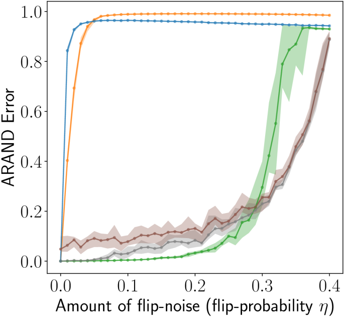
a) $k=20$, $p=0.1$

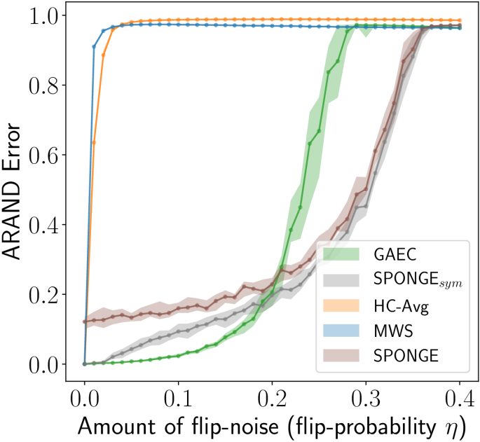
b) $k=50$, $p=0.2$

Figure 2: ARAND errors (median values over 20 experiments, lower is better) on synthetic graphs generated with SSBM. We consider $k$ ground truth communities of random size. Graphs have $N=10000$ nodes; edges are randomly added with probability $p$.

Scores on CREMI instance-segmentation – SSBM graphs are non-planar, and every edge has the same probability to be present in the graph. On the other hand, the gridGraph and 3D-RAG graphs of Table 2 are sparse and have a very regular structure: regardless of whether a node represents a pixel or a superpixel, it will only have edge connections with its neighbors in the image (up to a certain hop distance). Tables 3a)-3b) show that average linkage methods (HC-Avg, HCC-Avg) strongly outperform other methods on CREMI-gridGraph instances and also achieve the best scores on CREMI-3D-rag graphs. Sum-based linkage methods (GAEC, HCC-Sum) have a two times higher ARAND error on grid-graphs and often return under-clustered segments (see failure cases in Fig. 4). This suggests that the flooding strategy observed previously in the sum-linkage methods does not work on grid-graphs, because in this setup edge weights are predicted by a CNN and noise is strongly spatially-correlated . To fully test this hypothesis, we conduct a set of experiments where the CNN predictions are perturbed by adding structured noise and simulating additional artifacts like “holes” in the boundary evidence. The plot in Fig. 5 confirms that HC-Avg and HCC-Avg are very robust algorihtms on this data, followed by Sum-linkage algorithms and the Mutex Watershed algorithm (MWS). It is not a surprise that the AbsMax linkage used by MWS is not robust to this type of structured noise. However, the scores and runtimes in Table 3a) prove how MWS can achieve high accuracy with 70% lower runtime compared to HC-Avg.

Complete and Single Linkage – We use these two linkage methods as baselines to highlight the difficulty of the studied graph clustering problems listed in Table 2. Scores in Tables 3a)-3b) show their poor performance: Single linkage hierarchical clustering (HC-Single), which here is equivalent to thresholding the edge weights at $w_{e}=0$ and computing connected components in the graph, often returned few big under-segmented clusters. HC-Complete returned instead a lot of over-segmented clusters.

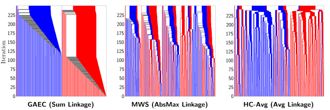
Figure 3: Clustering dynamics and accuracy of GASP variations on stochastic block models. The dendrograms result from three versions of GASP on a synthetic graph generated with SSBM ($250$ nodes, edge probability $p=0.05$, flipping probability $\eta=0.1$). Red and blue colors show which of the two equal-sized ground-truth communities each node belongs to. At the top, dendrograms are truncated at the level of the final clustering $\Pi^{*}$ returned by GASP.

Results on CREMI challenge – Table 3c) shows that the HCC-Avg and HC-Avg clustering algorithms achieve state-of-the-art accuracy on the CREMI challenge, when combined with predictions of our CNN. Most of the other entries (apart from LSI-Masks [6]) employ super-pixels based post-processing pipelines and cluster 3D-region-adjacency graphs. As we show in Table  3b), using superpixels considerably reduces the size of the clustering problem and, consequently, the post-processing time. However, our method operating directly on pixels (gridGraph + HCC-Avg) achieves better performances than superpixel-based methods (3D-RAG + HCC-Avg) and does not require the parameter tuning necessary to obtain good super-pixels, which is usually highly dataset dependent. To scale up our method operating on pixels, we divided each test-volume into four sub-blocks, and then combined the resulting clusterings by running the algorithms again on the combined graph. The method 3D-RAG + LiftedMulticut based on the lifted multicut approximation of [10] achieves the best scores overall, but it takes into account different information through the lifted edge weights that also depend on additional raw-data and shape information from highly engineered super-pixels.

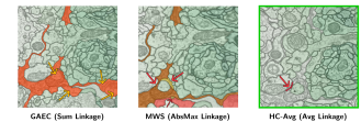
Figure 4: Failure cases of three versions of GASP applied to neuron segmentation. Only wrongly segmented regions are highlighted in different warm colors. Red arrows point to wrongly split regions; yellow arrows point to false merge errors. HC-Avg returned the best segmentation. Data is 3D, hence the same color could be assigned to parts of segments that appear disconnected in 2D.

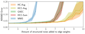
Figure 5: ARAND errors (median values over 20 experiments, lower is better) on CREMI-gridGraph clustering problems perturbed with structured noise. Average-linkage algorithms proved to be the most robust.

5 Conclusion

We have presented a unifying framework for agglomerative clustering of graphs with both positive and negative edge weights. This framework allowed us to explore new combinations of constraints and linkage criteria and to perform a consistent evaluation of all algorithms in it. We have then analyzed several theoretical and empirical properties of these algorithms. On instance segmentation, algorithms based on an average linkage criterion outperformed all the others: they proved to be simple and robust approaches to process short- and long-range predictions of a CNN. On biological images, these simple average agglomeration algorithms achieve state-of-the-art results without requiring the user to spend much time tuning complex task-dependent pipelines based on super-pixels.

A6 Appendix

A6.1 Implementation and complexity of GASP

Update rules

During the agglomerative process, the interaction between adjacent clusters has to be properly updated and recomputed, as shown in Algorithm 1. An efficient way of implementing these updates can be achieved by representing the agglomeration as a sequence of edge contractions in the graph. Given a graph $\mathcal{G}(V,E,w)$ and a clustering $\Pi$, we define the associated contracted graph $\tilde{\mathcal{G}}_{\Pi}(\tilde{V},\tilde{E},\tilde{w})$, such that there exists exactly one representative node $|\tilde{V}\cap S|=1$ for every cluster $S\in\Pi$ . Edges in $\tilde{E}$ represent adjacency-relationships between clusters and the signed edge weights $\tilde{w}_{e}$ are given by inter-cluster interactions $\tilde{w}(e_{uv})=\mathcal{W}_{S_{u}\cup S_{v}}$, where $S_{u}$ denotes the clustering including node $u$. For the linkage criteria tested in this article, when two clusters $S_{u}$ and $S_{v}$ are merged, the interactions between the new cluster $S_{u}\cup S_{v}$ and each of its neighbors depend only on the previous interactions involving $S_{u}$ and $S_{v}$. Thus, we can recompute these interactions by using an update rule $f$ that does not involve any loop over the edges of the original graph $\mathcal{G}$:

$$\mathcal{W}(S_{u}\cup S_{v}\cup S_{t})= f\Big{[}\mathcal{W}(S_{u}\cup S_{t}),\mathcal{W}(S_{v}\cup S_{t})\Big{]}$$ (5)

$$= f(\tilde{w}(e_{ut}),\tilde{w}(e_{vt}))$$ (6)

In Fig. A6 we show an example of edge contraction and in Table A4 we list the update rules associated to the linkage criteria we introduced in Table 1.

Implementation

Our implementation of GASP is based on an union-find data structure and a heap allowing deletion of its elements. In Phases 2 and 3, GASP is equivalent to a standard hierarchical agglomerative clustering algorithm with complexity $\mathcal{O}(N^{2}\log N)$. In Algorithm LABEL:detailed_alg, we show our implementation of phase 1, involving cannot-link constraints. In phase 1, the algorithm starts with each node assigned to its own cluster and sorts all edges $e\in E$ in a heap/priority queue (PQ) by their absolute weight $|w_{e}|=|w_{e}^{+}-w_{e}^{-}|$ in descending order, so that the most attractive and the most repulsive interactions are processed first. It then iteratively pops one edge $e_{uv}$ from PQ and, depending on the priority $\tilde{w}_{uv}$, does the following: in case of attractive interaction $\tilde{w}_{uv}>0$, provided that $e_{uv}$ was not flagged as a cannot-link constraint, merge the connected clusters, perform an edge contraction of $e_{uv}$ in $\tilde{\mathcal{G}}_{\Pi}$ and update the priorities of new double edges as explained in Fig. A6. If, on the other hand, the interaction is repulsive ($\tilde{w}_{uv}\leq 0$) and the option addCannotLinkContraints of Alg. LABEL:detailed_alg is True, then the edge $e_{uv}$ is flagged as cannot-link constraint.

Linkage criteria	Update rule $f$
Sum:	$f(\tilde{w}_{1},\tilde{w}_{2})=\tilde{w}_{1}+\tilde{w}_{2}$
Absolute Maximum:	$f(\tilde{w}_{1},\tilde{w}_{2})=\begin{cases}\tilde{w}_{1}&\text{if}\,\,|\tilde{w}_{1}|>|\tilde{w}_{2}|\\ \tilde{w}_{2}&\text{otherwise}\end{cases}$
Average:	$f(\tilde{w}_{1},\tilde{w}_{2})=\mathrm{weightAvg}\{\tilde{w}_{1},\tilde{w}_{2}\}$
Single:	$f(\tilde{w}_{1},\tilde{w}_{2})=\max\{\tilde{w}_{1},\tilde{w}_{2}\}$
Complete:	$f(\tilde{w}_{1},\tilde{w}_{2})=\min\{\tilde{w}_{1},\tilde{w}_{2}\}$

Table A4: The table lists the update rules $f(\tilde{w}_{1},\tilde{w}_{2})$ associated to the linkage criteria of Table 1 and that are used to efficiently update the interactions between clusters.

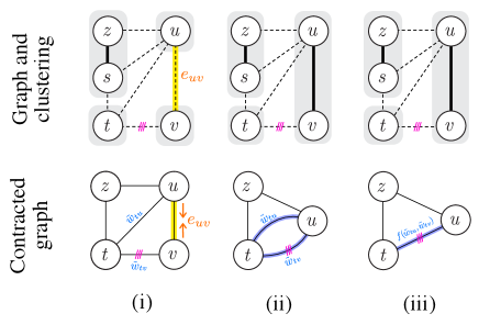
Figure A6: Example of edge contraction. First row: original graph $\mathcal{G}$; clustering $\Pi$ (gray shaded areas) with dashed edges on cut; cannot-link constraints (violet bars). Second row: contracted graph $\tilde{\mathcal{G}}_{\Pi}$. In step ii), edge $e_{uv}$ is contracted and node $v$ deleted from $\tilde{\mathcal{G}}_{\Pi}$. In step iii), double edges $e_{tu}$ and $e_{tv}$ resulting from the edge contraction are replaced by a single edge with updated interaction.

Complexity

In the main loop of Phase 1, the algorithm iterates over all edges, but the only iterations presenting a complexity different from $\mathcal{O}(1)$ are the ones involving a merge of two clusters, which are at most $N-1$. By using a union-find data structure (with path compression and union by rank) the time complexity of merge$(u,v)$ and find($u$) operations is $\mathcal{O}(\alpha(N))$, where $\alpha$ is the slowly growing inverse Ackerman function. The algorithm then iterates over the neighbors of the merged cluster (at most $N$) and updates/deletes values in the priority queue ($\mathcal{O}(\log|E|)$). Therefore, similarly to a heap-based implementation of hierarchical agglomerative clustering, our implementation of GASP - Phase 1 has a complexity of $\mathcal{O}(N^{2}\log N)$. In the worst case, when the graph is dense and $|E|=N^{2}$, the algorithm requires $\mathcal{O}(N^{2})$ memory. Nevertheless, in our practical applications the graph is much sparser, so $\mathcal{O}(|E|)=\mathcal{O}(N)$. With a single-linkage, corresponding to the choice of the Maximum update rule in our framework, the algorithm can be implemented by using the more efficient Kruskal’s Minimum Spanning Tree algorithm with complexity $\mathcal{O}(N\log N)$, but only when cannotLinkConstraints are not used. Moreover, GASP with Absolute Maximum linkage can be implemented more efficiently (see next section).

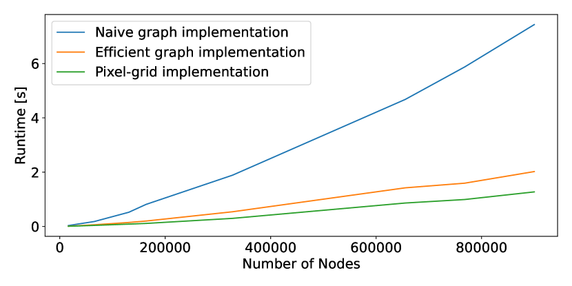
Figure A7: Runtimes for different implementation of GASP with AbsMax linkage criterion. Runtimes are averaged over 5 runs.

Efficiency of different GASP implementations with AbsMax linkage criteria

In Fig. A7, we compare the runtimes of three implementations of the AbsMax criteria: the implementation from [74] for pixel graphs (Pixel-grid implementation) and for general graphs (Efficient graph implementation) as well as the HC implementation with AbsMax linkage (Naive graph implementation). The specialized implementations can exploit the properties of the underlying graph and are faster. But our generalization does not carry a large computational penalty and only requires a few extra seconds for partitioning graphs of a million nodes. Note that we have always used the most efficient implementation for the results reported in the paper. We will clarify this fact.

Median linkage

We implemented median linkage in our library from the beginning but did not report on it in the main paper for two reasons: we consider the other criteria to span the range of interesting behavior well; and it performs no better than some of the other criteria (like average linkage) which are faster to evaluate.

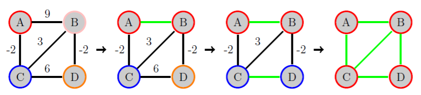
Figure A8: GASP agglomeration with the Abs Max criterion: contracted edges are marked green. The last contraction increases the MC objective from -1 to 0.

A6.2 GASP relation to the multicut objective

For some of the linkage criteria, e.g. sum and average, GASP can be understood as a local search to the objective of the multicut optimization problem 1, see [51]. But this does not hold in general: the Abs Max linkage for example does not always decrease the MC objective (see counter example in Fig. A8). Moreover, GASP cannot be seen as a k-approximation, because it is a polynomial algorithm and Chawla, et al. Computational complexity, 2006 has shown that approximating the multicut objective with any constant factor is in itself NP-hard.

A6.3 Proofs of Propositions 3.1, 3.2, A6.1, and 3.3

Lemma A6.1.

If GASP Algorithm 1 with Complete linkage criteria enforces a constraint between two clusters in Phase 1, then the interaction between the clusters will never become positive over the course of the following agglomeration steps.

Proof.

Two clusters are constrained in Phase 1 only if their interaction is repulsive and, with complete linkage, the signed interaction between two clusters can only decrease over the course of the agglomeration. Thus, if two clusters are constrained by the algorithm, their negative interaction cannot increase and become positive later on in the agglomeration process. ∎

Lemma A6.2.

If GASP Algorithm 1 with AbsMax linkage criteria enforces a constraint between two clusters in Phase 1, then the interaction between the clusters will never become positive over the course of the following agglomeration steps.

Proof.

During the agglomeration the interaction between two clusters can only increase in absolute value. Thus, the negative interaction $\mathcal{W}{}(S_{i}\cup S_{j})<0$ between two constrained clusters can possibly become positive over the course of next agglomeration steps only if there is at least another pair of clusters in the graph that has a positive interaction $\mathcal{W}{}(S_{l}\cup S_{t})>0$ higher in absolute value: $|\mathcal{W}{}(S_{l}\cup S_{t})|>|\mathcal{W}{}(S_{i}\cup S_{j})|$. If such clusters $S_{l},S_{t}$ with positive interaction exist, we note that they must also be constrained (in the opposite case, the algorithm would have already merged them before to constrain $S_{i}$ and $S_{j}$, because their priority is higher). In other words, a constrained negative interaction can become positive only if there is already another positive constrained interaction: but this can never be the case because initially all constrained interactions are negative. ∎

Lemma A6.3.

In the GASP Algorithm 1 with AbsMax or Complete linkage criteria (see linkage definition in Table 1), the same final clustering is returned whether or not cannot-link constraints are enforced.

Proof.

In phase 1 of Algorithm LABEL:detailed_alg, two clusters are merged only if the condition at line 9 is satisfied (i.e. when an interaction is both positive and not constrained). From Lemma A6.2 and Lemma A6.2 follows that with Complete and AbsMax linkage an interaction can never be both positive and constrained at the same time, so we directly conclude that the constrained and unconstrained versions of the algorithm will perform precisely the same agglomeration steps in phase 1. In phase 2 (after constraints have been removed) no clusters are merged because all interactions are already negative (whether they previously constrained or not). Thus, both constrained and unconstrained versions of GASP return the same clustering $\Pi^{*}$. ∎

See 3.1

Proof.

From Lemma A6.3 it directly follows that GASP with AbsMax linkage criterion returns the same final clustering whether or not cannot-link constraints are enforced. In the following, we prove that MWS (see pseudocode LABEL:alg:mutex_watershed) and the constrained AbsMax version of GASP also return the same clustering. Both algorithms sort edges in descending order of the absolute interactions $|w_{e}|$ and then iterate over all of them. The only difference is that MWS, after merging two clusters, does not update the interactions between the new cluster and its neighbors. However, since with an Abs. Max. linkage the interaction between clusters is simply given by the edge with highest absolute weight $|w_{e}|$, the order by which edges are iterated over in GASP is never updated. Thus, both algorithms perform precisely the same steps and return the same clustering. ∎

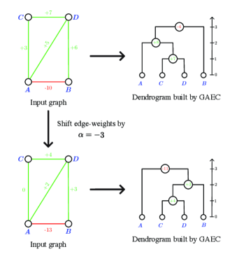
Figure A9: Counter-example showing that GAEC is not weight-shift invariant.

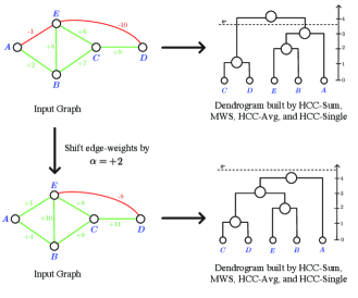
Figure A10: Counter-example showing that HCC-Sum, MWS, HCC-Avg, and HCC-Single are not weight-shift invariant.

See 3.2

Proof.

Theorem 1 in [12] proves that hierarchical clustering with Average (HC-Avg), Single (HC-Single), and Complete linkage (HC-Complete) are weight-shift invariant.

The same is not true for GASP with Sum linkage criteria (GAEC and HCC-Sum), because by adding a constant $\alpha$ to all edge weights $w_{e}$, the interaction between two clusters $S_{i}$ and $S_{j}$ is increased by a factor $\alpha|E_{ij}|$, which depends on the number of edges $|E_{ij}|$ connecting the two clusters. Thus, when all edge weighs of the graph are shifted, the agglomeration order may change. For a simple example of this, it is enough to consider the toy graph in Fig. 1a and shift the weights of the graph by $\alpha=-3$ (see Fig. A9).

The constrained versions of GASP (HCC-Avg and HCC-Single) are also not weight-shift invariant: here, the algorithm merges or constrains clusters in a given order, depending on the absolute interactions $|\mathcal{W}{}(S_{i}\cup S_{j})|$ between clusters; so, when edge weights are shifted by a constant $\alpha$, the sorting by absolute value can change arbitrarily together with the agglomeration order, as we show in the counter-example of Fig. A10. Similarly, the Mutex Watershed algorithm is not weight-shift invariant because it uses a linkage criterion that compares weights by their absolute values (see again counter-example in Fig. A10. ∎

Proposition A6.1.

Consider a graph $\mathcal{G}(V,E,w_{e})$, a linkage criterion $\mathcal{W}{}$, and an agglomerative algorithm returning a binary rooted tree $T$ with height $h_{T}$. Then, $(V,d_{T})$ defined in Eq. 3 is an ultrametric if and only if the following is true:

$$\forall u,v,t\in V$$

$$h_{T}(u,v)<h_{T}(u,t)\Rightarrow\mathcal{W}{}_{T}(u,v)\geq\mathcal{W}{}_{T}(u,t)$$ (7)

In words, condition 7 means: if the algorithm merges nodes $u,v$ before to merge nodes $u,t$, then the signed interaction $\mathcal{W}{}_{T}(u,v)$ between $u$ and $v$ has to be higher or equal than $\mathcal{W}{}_{T}(u,t)$.

Proof.

From the definition of $d_{T}$, it follows that:

$$d_{T}(u,u) =0\qquad \forall u\in V$$ (8)

$$d_{T}(u,v) \geq 0\qquad \forall u,v\in V$$ (9)

$$d_{T}(u,v) =d_{T}(v,u)\qquad \forall u,v\in V.$$ (10)

In order to show that $(V,d_{T})$ is an ultrametric, we only need to prove the ultrametric property:

$$d_{T}(u,v)\leq\max\{d_{T}(u,t),d_{T}(v,t)\}\quad\forall u,v,t\in V.$$ (11)

When at least two of the three nodes $u,v,t\in V$ are the same, this property follows from Eq. 8 and Eq. 9. When nodes $u,v,t\in V$ are distinct, from the definition of $d_{T}$ it follows that Eq. 11 is equivalent to:

$$\mathcal{W}{}_{T}(u,v)\geq\min\{\mathcal{W}{}_{T}(u,t),\mathcal{W}{}_{T}(v,t)\}.$$ (12)

In the following, we prove both sides of the if and only if statement in the proposition. First, we prove the $(\Leftarrow)$ side, i.e. that if assumption 7 holds, then $(V,d_{T})$ is an ultrametric and 12 holds.

Case 1: in Eq. 12, $t\in V$ is part of the sub-tree ${T[u\vee v]}$. In other words, the algorithm first merges node $t$ with either node $u$ or $v$, and then $u$ and $v$ are merged together. Let us assume that $t$ is first merged with $u$ (the following proof also holds for the opposite case in which $t$ is first merged with $v$):

$$h_{T}(u,t)<h_{T}(u,v)=h_{T}(v,t).$$ (13)

Thus, by combining the last equation with assumption (7), it follows that

$$\mathcal{W}{}_{T}(u,t)\geq\mathcal{W}{}_{T}(v,t)\quad\text{and}\quad\mathcal{W}{}_{T}(u,v)=\mathcal{W}{}_{T}(v,t)$$ (14)

and Eq. 12 follows (becoming an equality in this case).

Case 2: in Eq. 12, $t\in V$ is not part of the sub-tree ${T[u\vee v]}$. Thus, the algorithm first merges nodes $u$ and $v$, and then it merges node $t$ together with the cluster containing $u$ and $v$:

$$h_{T}(u,v)<h_{T}(u,t)=h_{T}(v,t).$$ (15)

Thus, from assumption 7 we have that

$$\mathcal{W}{}_{T}(u,v)\geq\mathcal{W}{}_{T}(u,t)\quad\text{and}\quad\mathcal{W}{}_{T}(u,v)\geq\mathcal{W}{}_{T}(v,t),$$ (16)

so also in this case Eq. 12 follows.

Next, we are left to prove the $(\Rightarrow)$ side of the if and only if statement: if $(V,d_{T})$ is an ultrametric, then assumption 7 holds. To prove this statement, we first rephrase it in the following equivalent form: if assumption 7 does not hold, then $(V,d_{T})$ is not an ultrametric and 12 does not hold. If we negate assumption 7, there must be at least three $u,v,t\in V$ such that:

$$h_{T}(u,v)<h_{T}(u,t)\quad\text{and}\quad\mathcal{W}{}_{T}(u,v)<\mathcal{W}{}_{T}(u,t).$$ (17)

The first condition, in words, is again assuming that the algorithm first merges nodes $u$ and $v$, and later it also merges node $t$ with the cluster containing $u$ and $v$. Thus, we can rephrase this assumption as:

$$\mathcal{W}{}_{T}(u,v)<\mathcal{W}{}_{T}(u,t)=\mathcal{W}{}_{T}(v,t).$$ (18)

From this, it follows that

$$\mathcal{W}{}_{T}(u,v)<\min\{\mathcal{W}{}_{T}(u,t),\mathcal{W}{}_{T}(v,t)\},$$ (19)

which is exactly the negation of the ultrametric property 12. ∎

See 3.3

Proof.

Thanks to Prop. A6.1, we know that $(V,d_{T^{*}})$ is an ultrametric if and only if assumption 7 holds. Thus, in the following, we will prove which variations of the GASP Algorithm 1 satisfy assumption 7. In other words, we need to prove in which cases GASP merges clusters according to a monotonously decreasing order of signed interactions $\mathcal{W}{}$.

GASP puts clusters in a priority queue (Algorithm 1, lines 5 and 15) and merges them starting from those with the highest interaction (lines 9, 19, and 26). However, the priority queue is updated each time two clusters are merged (lines 10, 20, and 27). Thus, to ensure a monotonously decreasing merging order, updated interactions involving a merged cluster should always be lower or equal than previously existing interactions (condition 1):

$$\forall S_{i}\in\Pi\setminus\{S_{1},S_{2}\},$$

$$\mathcal{W}{}(S_{1}\cup S_{2}\cup S_{i}) \leq\max\{\mathcal{W}{}(S_{1}\cup S_{i}),\mathcal{W}{}(S_{2}\cup S_{i})\}$$ (20)

where $\Pi$ is a clustering, $\mathcal{W}{}$ is a linkage criteria, and $S_{1},S_{2}\in\Pi$ are two clusters merged by the algorithm at a given iteration. If this condition is true then, in the following iterations, GASP can only merge clusters with lower (or equal) interaction values.

We also note that, in phase 1, the algorithm skips interactions that are both positive and constraint (condition at line 8 in Algorithm 1) and merges them only later in phase 2 (line 19), when constraints are removed. Clearly, whenever this happens, a decreasing merging order is no longer ensured. Thus, on top of condition 1, we also have that no merging decisions should be “delayed” from phase 1 to phase 2 (condition 2).

Condition 1 always holds for Average, Single, Complete, and AbsMax linkage criteria, but not for a Sum linkage criteria, because the sum of two positive numbers $a,b$ is always higher than $\max\{a,b\}$. This is also demonstrated in the toy example of Fig. 1a, proving that, in general, Sum-linkage algorithms like GAEC or HCC-Sum do not define an ultrametric on the graph.

Thanks to Lemma A6.3, we have that condition 2 always holds for algorithms based on AbsMax and Complete linkage, proving that the Mutex Watershed and HC-Complete algorithms define an ultra-metric (whether or not cannot-link-constraints are enforced). On the other hand, condition 2 does not hold for other variations of GASP involving cannot-link-constraints (HCC-Sum, HCC-Avg, and HCC-Single), which do not then define an ultrametric.

Finally, the remaining not constrained versions of GASP (HC-Avg, HC-Single, and HC-Complete) satisfy both conditions, so they define an ultrametric, confirming the well-known results of related work in hierarchical clustering on unsigned graphs [33, 58].

∎

A6.4 Mutex Watershed on SSBM graphs

Proposition A6.2.

Consider a graph generated by an Erdős-Rényi signed stochastic block model (SSBM) as described in Section 4.1, with $N$ nodes, edges added with probability $p$, sign-flip probability $\eta<0.5$, $k$ ground-truth clusters, and edge weights Gaussian-distributed with standard deviation $\sigma$. Then, at every iteration, GASP with Absolute Maximum linkage (or, in other words, the Mutex Watershed algorithm) always makes a mistake with at least probability $\eta$.

Proof.

Thanks to Lemma A6.3 we know that GASP with Absolute Maximum linkage returns the same clustering whether or not cannot-link-constraints are used. Thus, in the following, we prove the proposition considering the version enforcing constraints. Let us consider a generic iteration of the algorithm, where two clusters $S_{\alpha}$ and $S_{\beta}$ have the highest priority and are popped from priority queue. Then, the MWS algorithm will either merge or constrain them depending on the fact that their interaction $\mathcal{W}_{\mathrm{AbsMax}}(S_{\alpha}\cup S_{\beta})$ is positive or negative (note that, with AbsMax linkage, an interaction can never be positive and constrained, as shown in Lemma A6.3). By construction of the SSBM, every edge $e\in E$ in the graph has a absolute weight distributed as $|w_{e}|\sim\mathcal{N}(1,\sigma^{2})$. Thus, every edge $e^{\prime}\in(S_{\alpha}\times S_{\beta})\cap E$ connecting the two clusters has the same probability to have the highest absolute weight, and the sign of the interaction $\mathcal{W}_{\mathrm{AbsMax}}(S_{\alpha}\cup S_{\beta})$ will only depend on the sign of this highest edge. Therefore, the probability that the MWS merges two clusters is simply given by the fraction of positive weighted edges connecting them.

Let $\tilde{\Pi}=\{\tilde{S}_{1},\ldots,\tilde{S}_{k}\}$ denote the ground truth clustering, and $\tilde{S}_{\alpha i}=S_{\alpha}\cap\tilde{S}_{i}$ denote the intersection between cluster $S_{\alpha}$ and a ground-truth cluster $\tilde{S}_{i}$. If the generated graph is dense, i.e. $p=1$, then the total number of edges connecting clusters $S_{\alpha}$ and $S_{\beta}$ that have a true attractive or repulsive weight is (according to the ground truth labels)

$$\Gamma^{+}=\sum_{i=1}^{k}|\tilde{S}_{\alpha i}||\tilde{S}_{\beta i}|,\quad\Gamma^{-}=\sum_{i=1}^{k}\sum_{j=1,j\neq i}^{k}|\tilde{S}_{\alpha i}||\tilde{S}_{\beta j}|.$$ (21)

When the edges in the graph are randomly added with a probability $p$, then the actual number of true attractive and repulsive interactions connecting the two clusters is (according to the ground truth labels):

$$\gamma^{+}\sim\mathcal{B}(\Gamma^{+},p),\qquad\gamma^{-}\sim\mathcal{B}(\Gamma^{-},p),$$ (22)

where $\mathcal{B}(\Gamma,p)$ is the binomial distribution:

$$\mathcal{B}(\gamma;\Gamma,p)=\frac{\Gamma!}{\gamma!(\Gamma-\gamma)!}p^{\gamma}(1-p)^{\Gamma-\gamma}.$$ (23)

Here, we only assume that $\gamma^{+}+\gamma^{-}>0$, i.e. there is at least one edge connecting the two clusters (otherwise their interaction would be zero and the MWS would not have popped them from priority queue).

So far we have been talking about attractive and repulsive connections according to the ground truth labels. In our SSBM however every edge has a uniform probability $\eta$ to have its sign flip, so the actual number of attractive interactions connecting the two clusters will be instead given by the sum of the true attractive interactions $\gamma^{+}_{\mathrm{nf}}\sim\mathcal{B}(\gamma^{+},1-\eta)$ that have not been flipped, plus the true negative interactions $\gamma^{-}_{\mathrm{f}}\sim\mathcal{B}(\gamma^{-},\eta)$ that have been flipped. Putting everything together, given two clusters with $\gamma^{+}$ true attractive interactions and $\gamma^{-}$ true negative ones, the highest-absolute-weight edge connecting them has the following probability to be positive:

$$\mathbb{P}[\mathcal{W}_{\mathrm{AbsMax}} (S_{\alpha}\cup S_{\beta})>0;\gamma^{+},\gamma^{-}]=$$

$$= \sum_{\gamma^{+}_{\mathrm{nf}}=0}^{\gamma^{+}}\sum_{\gamma^{-}_{\mathrm{f}}=0}^{\gamma^{-}}\mathcal{B}(\gamma^{-}_{\mathrm{f}};\gamma^{-},\eta)\mathcal{B}(\gamma^{+}_{\mathrm{nf}};\gamma^{+},1-\eta)\cdot$$

$$\qquad\qquad\cdot\left(\frac{\gamma^{+}_{\mathrm{nf}}+\gamma^{-}_{\mathrm{f}}}{\gamma^{+}+\gamma^{-}}\right)$$

$$\stackrel{{\scriptstyle(*)}}{{=}} \frac{\gamma^{+}(1-\eta)+\gamma^{-}\eta}{\gamma^{+}+\gamma^{-}}$$ (24)

where in $(*)$ we used the fact that the expected value of a binomial distribution $\mathcal{B}(\gamma,\eta)$ is $\gamma\eta$.

Now we note that this probability is bounded in the interval $[\eta,1-\eta]$. So, regardless of whether the two clusters $S_{\alpha}$ and $S_{\beta}$ should be merged or constraint according to ground truth labels, the probability not to make the correct decision is always at least $\eta$. Remarkably, while the exact probability in Eq. A6.4 depends on the number of edges connecting the two clusters $\gamma^{+}+\gamma^{-}$ and thus on the cluster sizes, the bounds do not. Thus, this result shows that, unlike Sum or Avg linkage methods, the MWS algorithm is unable to reliably correct for the sign flip noise even for big clusters linked by many edges. ∎

A6.5 Application to neuron segmentation

Training and data augmentation

The data from the CREMI challenge is highly anisotropic and contains artifacts like missing sections, staining precipitations and support film folds. To alleviate difficulties stemming from misalignment, we use a version of the data that was elastically realigned by the challenge organizers with the method of S. Saalfeld, et al. Nature methods, 2012. In addition to the standard data augmentation techniques of random rotations, random flips and elastic deformations, we simulate data artifacts. We randomly zero-out slices, decrease the contrast of slices, simulate tears, introduce alignment jitter and paste artifacts extracted from the training data. Both [28] and [50] have shown that these kinds of augmentations can help to alleviate issues caused by EM-imaging artifacts. We use L2 loss and Adam optimizer to train the network. The model was trained on all three samples with available ground truth labels.

CREMI-gridRag instances

Our 3D UNet model predicts the same set of 12 long-and-short range affinities as described in [50]. When building the pixel-grid graph, we add both direct neighbors connections and the long-range connections predicted by our model (every voxel is connected to other six voxels via direct connections and other 18 voxels via long-range edges). Empirically, when long-range predictions of the CNN are added as long-range connections in the graph, GASP achieves better scores as compared to when only direct-neighbors predictions are used. Our intuitive explanation of this is that, where there is a clear boundary evidence between two segments, the long-range predictions of the CNN model are more certain than the direct-neighbor ones, because it is often impossible to estimate the exact ground-truth label transition for pixels that are very close to a boundary evidence. However, empirically, we also find that GASP achieves the best scores when only 10% of the long-range connections are randomly sampled and added to the grid-graph. When all the long-range connections predicted by the CNN are added to the graph (18 connections for every voxel), all versions of GASP tend to perform more over-clustering errors. In practice, we explain this by observing that many challenging parts of the studied neuron segmentation data involve thin and elongated segments, and our model sometimes fails to connect distant pairs of pixels that, according to the ground-truth labels, should belong to the same segment (even though, in this case, the direct neighboring predictions are correct). To sum up, the scores we report in Tables 3a) are obtained by using only 10% of the long-range predictions, since this was the setup that performed the best. After running GASP, we use a simple post-processing step to delete small segments on the boundaries, most of which are given by single-voxel clusters. On the neuron segmentation predictions, we deleted all regions with less than 200 voxels and used a seeded watershed algorithm to expand the bigger segments.

CREMI-3D-rag instances

We build these clustering problems by generating superpixels and then building a 3D region adjacency graph. Due to the anisotropy of the data, we generate 2D superpixels by considering each 2D image in the stack singularly. First, we generate a boundary-evidence map by taking an average over the two direct-neighbor predictions of the CNN model (one for each direction in the 2D image of the stack) and applying some additional smoothing. Then, we threshold the boundary map, compute a distance transform, and run a watershed algorithm seeded at the maxima of the distance transform (WSDT). The degree of smoothing was optimized such that each region receives as few seeds as possible, without however causing severe under-segmentation. The computed 2D superpixels are then used to build a 3D region-adjacency graph (3D-rag). The weights of the edges are given by averaging the CNN affinities over the boundaries of adjacent superpixels.

Clustering problem	GAEC [39]	HCC-Sum	MWS [75]	HC-Avg	HCC-Avg	HC-Single	HCC-Single	HC-Complete
Modularity Clustering	-0.457	-0.453	-0.073	-0.467	-0.467	0.000	0.000	-0.201
Image Segmentation	-2,955	-2,953	-2,901	-2,903	-2,896	-1,384	-1,384	-2,102
Knott-3D (150-300-450)	-36,667	-36,652	-35,200	-35,957	-35,631	-2,522	-2,522	30,629
CREMI-3D-rag	-1,112,287	-1,112,286	-1,109,731	-1,112,177	-1,112,100	-1,038,709	-1,038,709	-748,734,869
Fruit-Fly Level 1-4	-151,022	-151,017	-150,879	-150,909	-150,876	-71,477	-71,997	-128,733
CREMI-gridGraph	-73,317,601	-73,328,867	-73,330,568	-73,502,947	-73,474,856	-45,194,180	-45,194,443	311,598,700
Fruit-Fly Level Global	-151,688	-151,596	-146,315	-150,466	-150,171	-4,422	-	6,876

Table A5: We compare algorithms in the GASP framework by evaluating which of the obtained clusterings is associated to the lowest value of the multicut objective defined in Eq. 1 (lower is better). Single and complete linkage methods performed much worse than the others. Note that HCC-Single is the algorithm with the highest runtime (see Table 3a)) and it did not scale up to the very large clustering problem Fruit-Fly Level Global.

A6.6 Adding structured noise to CNN predictions

Additionally to the comparison on the full training dataset, we performed more experiments on a crop of the more challenging CREMI training sample B, where we perturbed the predictions of the CNN with noise and we introduced additional artifacts like missing boundary evidences.

In the field of image processing there are several ways of adding noise to an image, among which the most common are Gaussian noise or Poisson shot noise. In these cases, the noise of one pixel does not correlate with its neighboring noise values. On the other hand, predictions of a CNN are known to be spatially correlated. Thus, we used Perlin noise, one of the most common gradient noises used in procedural pattern generation. This type of noise $n(x)\in[0,1]$ generates spatial random patterns that are locally smooth but have large and diverse variations on bigger scales. We then combined it with the CNN predictions $p(x)$ in the following way:

$$\tilde{F}(x;\mathcal{K})=F(x)+\mathcal{K}\cdot\max\left(N(x),0\right),$$ (25)

where $N(x)=\mathrm{Logit}[n(x)]$; $F(x)=\mathrm{Logit}[p(x)]$ and $\mathcal{K}\in\mathbb{R}^{+}$ is a positive factor representing the amount of added noise. The resulting perturbed predictions $\tilde{F}(x;\mathcal{K})$ are then under-clustering biased, such that the probability for two pixels to be in the same cluster is increased only if $N(x)>0$ (see Fig. A11b and A11c). Note that in these experiments we focused only on predictions perturbed with under-clustering biased noise (and not over-clustering biased noise). The reason is that generating realistic over-clustering biased CNN predictions is more complex and cannot be simply done by adding Perlin noise: as we show in Fig. A11c, by adding Perlin noise we can easily “remove” parts of a boundary evidence, but it is not possible to generate random new realistic boundary evidence.

In our experiments, each pixel is represented by a node in the grid-graph and it is linked to $n_{\mathrm{nb}}$ other nodes by short- and long-range edges. Thus, the output volume of our CNN model is a four-dimensional tensor with $n_{\mathrm{nb}}$ channels: for each pixel / voxel, the model outputs $n_{\mathrm{nb}}$ values representing affinities of different edge connections. We then generated a 4-dimensional Perlin noise tensor that matches the dimension of the CNN output. The data is highly anisotropic, i.e. it has a lower resolution in one of the dimensions. Due to this fact, we chose different smoothing parameters to generate the noise in different directions.

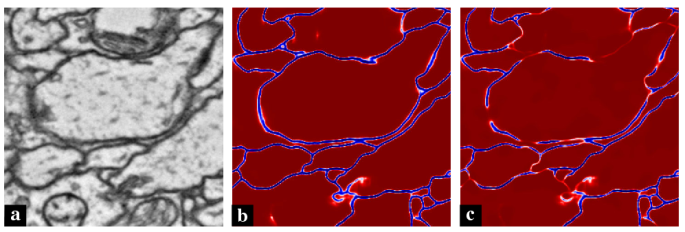
Figure A11: CNN predictions on a slice of the CREMI neuron segmentation challenge with and without additional spatially-correlated noise. (a) Raw data (b) Original CNN predictions $F(x)$, where blue pixels represent boundary evidence (c) Strongly perturbed version $\tilde{F}(x;\mathcal{K})$ of the predictions defined in Eq. 25 with $\mathcal{K}=8$. Long-range predictions are not shown.

Method	ARAND Error
HC-Avg (GASP with Avg Linkage)	0.1034
GAEC [39] (GASP with Sum Linkage)	0.1035
MWS [75] (GASP with AbsMax linkage)	0.1068
SPONGEsym [19]	0.4161
$L_{sym}$ [46]	0.8069
SPONGE [19]	0.9211
BNC [14]	0.9926

Table A6: GASP compared to spectral clustering methods on a small crop of the CREMI neuron segmentation dataset. Since spectral methods cannot scale to the full CREMI dataset, we evaluated them on a smaller $10\times 100\times 100$ sub-volume of CREMI training sample B. Despite the fact that the true number of ground truth clusters was given as an input to the spectral methods, GASP significantly outperformed them.

References

- [1] Bjoern Andres, Jörg H Kappes, Thorsten Beier, Ullrich Köthe, and Fred A Hamprecht. Probabilistic image segmentation with closedness constraints. In 2011 International Conference on Computer Vision, pages 2611–2618. IEEE, 2011.
- [2] Bjoern Andres, Thorben Kroeger, Kevin L Briggman, Winfried Denk, Natalya Korogod, Graham Knott, Ullrich Koethe, and Fred A Hamprecht. Globally optimal closed-surface segmentation for connectomics. In European Conference on Computer Vision, pages 778–791. Springer, 2012.
- [3] Pablo Arbelaez, Michael Maire, Charless Fowlkes, and Jitendra Malik. Contour detection and hierarchical image segmentation. IEEE transactions on pattern analysis and machine intelligence, 33(5):898–916, 2011.
- [4] Ignacio Arganda-Carreras, Srinivas C Turaga, Daniel R Berger, Dan Cireşan, Alessandro Giusti, Luca M Gambardella, Jürgen Schmidhuber, Dmitry Laptev, Sarvesh Dwivedi, Joachim M Buhmann, et al. Crowdsourcing the creation of image segmentation algorithms for connectomics. Frontiers in neuroanatomy, 9:142, 2015.
- [5] Min Bai and Raquel Urtasun. Deep watershed transform for instance segmentation. In Proceedings of the IEEE Conference on Computer Vision and Pattern Recognition, pages 5221–5229, 2017.
- [6] Alberto Bailoni, Constantin Pape, Steffen Wolf, Anna Kreshuk, and Fred A Hamprecht. Proposal-free volumetric instance segmentation from latent single-instance masks. arXiv preprint arXiv:2009.04998, 2020.
- [7] Nikhil Bansal, Avrim Blum, and Shuchi Chawla. Correlation clustering. Machine learning, 56(1-3):89–113, 2004.
- [8] Thorsten Beier, Björn Andres, Ullrich Köthe, and Fred A Hamprecht. An efficient fusion move algorithm for the minimum cost lifted multicut problem. In European Conference on Computer Vision, pages 715–730. Springer, 2016.
- [9] Thorsten Beier, Thorben Kroeger, Jorg H Kappes, Ullrich Kothe, and Fred A Hamprecht. Cut, glue & cut: A fast, approximate solver for multicut partitioning. In Proceedings of the IEEE Conference on Computer Vision and Pattern Recognition, pages 73–80, 2014.
- [10] Thorsten Beier, Constantin Pape, Nasim Rahaman, Timo Prange, Stuart Berg, Davi D Bock, Albert Cardona, Graham W Knott, Stephen M Plaza, Louis K Scheffer, et al. Multicut brings automated neurite segmentation closer to human performance. Nature Methods, 14(2):101, 2017.
- [11] Ulrik Brandes, Daniel Delling, Marco Gaertler, Robert Gorke, Martin Hoefer, Zoran Nikoloski, and Dorothea Wagner. On modularity clustering. IEEE transactions on knowledge and data engineering, 20(2):172–188, 2007.
- [12] Morteza Haghir Chehreghani. Hierarchical correlation clustering and tree preserving embedding. arXiv preprint arXiv:2002.07756, 2020.
- [13] Bowen Cheng, Maxwell D. Collins, Yukun Zhu, Ting Liu, Thomas S. Huang, Hartwig Adam, and Liang-Chieh Chen. Panoptic-DeepLab. arXiv preprint arXiv:1910.04751, 2019.
- [14] Kai-Yang Chiang, Joyce Jiyoung Whang, and Inderjit S Dhillon. Scalable clustering of signed networks using balance normalized cut. In Proceedings of the 21st ACM international conference on Information and knowledge management, pages 615–624. ACM, 2012.
- [15] Sunil Chopra and Mendu R Rao. On the multiway cut polyhedron. Networks, 21(1):51–89, 1991.
- [16] Sunil Chopra and Mendu R Rao. The partition problem. Mathematical Programming, 59(1-3):87–115, 1993.
- [17] Özgün Çiçek, Ahmed Abdulkadir, Soeren S Lienkamp, Thomas Brox, and Olaf Ronneberger. 3D U-Net: learning dense volumetric segmentation from sparse annotation. In International conference on medical image computing and computer-assisted intervention, pages 424–432. Springer, 2016.
- [18] Dan Ciresan, Alessandro Giusti, Luca M Gambardella, and Jürgen Schmidhuber. Deep neural networks segment neuronal membranes in electron microscopy images. In Advances in neural information processing systems, pages 2843–2851, 2012.
- [19] Mihai Cucuringu, Peter Davies, Aldo Glielmo, and Hemant Tyagi. SPONGE: A generalized eigenproblem for clustering signed networks. In AISTATS, 2019.
- [20] Mihai Cucuringu, Ioannis Koutis, Sanjay Chawla, Gary Miller, and Richard Peng. Simple and scalable constrained clustering: a generalized spectral method. In Artificial Intelligence and Statistics, pages 445–454, 2016.
- [21] Bert De Brabandere, Davy Neven, and Luc Van Gool. Semantic instance segmentation with a discriminative loss function. arXiv preprint arXiv:1708.02551, 2017.
- [22] Erik D Demaine, Dotan Emanuel, Amos Fiat, and Nicole Immorlica. Correlation clustering in general weighted graphs. Theoretical Computer Science, 361(2-3):172–187, 2006.
- [23] Alireza Fathi, Zbigniew Wojna, Vivek Rathod, Peng Wang, Hyun Oh Song, Sergio Guadarrama, and Kevin P Murphy. Semantic instance segmentation via deep metric learning. arXiv preprint arXiv:1703.10277, 2017.
- [24] Pedro F Felzenszwalb and Daniel P Huttenlocher. Efficient graph-based image segmentation. International journal of computer vision, 59(2):167–181, 2004.
- [25] Jenny Rose Finkel and Christopher D Manning. Enforcing transitivity in coreference resolution. In Proceedings of the 46th Annual Meeting of the Association for Computational Linguistics on Human Language Technologies: Short Papers, pages 45–48. Association for Computational Linguistics, 2008.
- [26] Jan Funke, Fred A Hamprecht, and Chong Zhang. Learning to segment: training hierarchical segmentation under a topological loss. In International Conference on Medical Image Computing and Computer-Assisted Intervention, pages 268–275. Springer, 2015.
- [27] Jan Funke, Stephan Saalfeld, Davi Bock, Srini Turaga, and Eric Perlman. Cremi challenge. https://cremi.org., 2016. Accessed: 2019-11-15.
- [28] Jan Funke, Fabian David Tschopp, William Grisaitis, Arlo Sheridan, Chandan Singh, Stephan Saalfeld, and Srinivas C Turaga. Large scale image segmentation with structured loss based deep learning for connectome reconstruction. IEEE transactions on pattern analysis and machine intelligence, 2018.
- [29] Naiyu Gao, Yanhu Shan, Yupei Wang, Xin Zhao, Yinan Yu, Ming Yang, and Kaiqi Huang. SSAP: Single-shot instance segmentation with affinity pyramid. In The IEEE International Conference on Computer Vision (ICCV), October 2019.
- [30] Martin Grötschel and Yoshiko Wakabayashi. A cutting plane algorithm for a clustering problem. Mathematical Programming, 45(1-3):59–96, 1989.
- [31] Martin Grötschel and Yoshiko Wakabayashi. Facets of the clique partitioning polytope. Mathematical Programming, 47(1-3):367–387, 1990.
- [32] Michał Januszewski, Jörgen Kornfeld, Peter H Li, Art Pope, Tim Blakely, Larry Lindsey, Jeremy Maitin-Shepard, Mike Tyka, Winfried Denk, and Viren Jain. High-precision automated reconstruction of neurons with flood-filling networks. Nature methods, 15(8):605, 2018.
- [33] Stephen C Johnson. Hierarchical clustering schemes. Psychometrika, 32(3):241–254, 1967.
- [34] Joerg Kappes, Bjoern Andres, Fred Hamprecht, Christoph Schnorr, Sebastian Nowozin, Dhruv Batra, Sungwoong Kim, Bernhard Kausler, Jan Lellmann, Nikos Komodakis, et al. A comparative study of modern inference techniques for discrete energy minimization problems. In Proceedings of the IEEE conference on computer vision and pattern recognition, pages 1328–1335, 2013.
- [35] Jörg Hendrik Kappes, Markus Speth, Björn Andres, Gerhard Reinelt, and Christoph Schnörr. Globally optimal image partitioning by multicuts. In International Workshop on Energy Minimization Methods in Computer Vision and Pattern Recognition, pages 31–44. Springer, 2011.
- [36] Amirhossein Kardoost and Margret Keuper. Solving minimum cost lifted multicut problems by node agglomeration. In ACCV 2018, 14th Asian Conference on Computer Vision, Perth, Australia, 2018.
- [37] Verena Kaynig, Amelio Vazquez-Reina, Seymour Knowles-Barley, Mike Roberts, Thouis R Jones, Narayanan Kasthuri, Eric Miller, Jeff Lichtman, and Hanspeter Pfister. Large-scale automatic reconstruction of neuronal processes from electron microscopy images. Medical image analysis, 22(1):77–88, 2015.
- [38] Brian W Kernighan and Shen Lin. An efficient heuristic procedure for partitioning graphs. Bell system technical journal, 49(2):291–307, 1970.
- [39] Margret Keuper, Evgeny Levinkov, Nicolas Bonneel, Guillaume Lavoué, Thomas Brox, and Bjorn Andres. Efficient decomposition of image and mesh graphs by lifted multicuts. In Proceedings of the IEEE International Conference on Computer Vision, pages 1751–1759, 2015.
- [40] B Ravi Kiran and Jean Serra. Global–local optimizations by hierarchical cuts and climbing energies. Pattern Recognition, 47(1):12–24, 2014.
- [41] Alexander Kirillov, Evgeny Levinkov, Bjoern Andres, Bogdan Savchynskyy, and Carsten Rother. Instancecut: from edges to instances with multicut. In Proceedings of the IEEE Conference on Computer Vision and Pattern Recognition, pages 5008–5017, 2017.
- [42] Seymour Knowles-Barley, Verena Kaynig, Thouis Ray Jones, Alyssa Wilson, Joshua Morgan, Dongil Lee, Daniel Berger, Narayanan Kasthuri, Jeff W Lichtman, and Hanspeter Pfister. RhoanaNet pipeline: Dense automatic neural annotation. arXiv preprint arXiv:1611.06973, 2016.
- [43] Iasonas Kokkinos. Pushing the boundaries of boundary detection using deep learning. arXiv preprint arXiv:1511.07386, 2015.
- [44] Shu Kong and Charless C Fowlkes. Recurrent pixel embedding for instance grouping. In Proceedings of the IEEE Conference on Computer Vision and Pattern Recognition, pages 9018–9028, 2018.
- [45] Nikola Krasowski, Thorsten Beier, Graham W Knott, Ullrich Koethe, Fred A Hamprecht, and Anna Kreshuk. Improving 3D EM data segmentation by joint optimization over boundary evidence and biological priors. In 2015 IEEE 12th International Symposium on Biomedical Imaging (ISBI), pages 536–539. IEEE, 2015.
- [46] Jérôme Kunegis, Stephan Schmidt, Andreas Lommatzsch, Jürgen Lerner, Ernesto W De Luca, and Sahin Albayrak. Spectral analysis of signed graphs for clustering, prediction and visualization. SIAM, 2010.
- [47] Jan-Hendrik Lange, Bjoern Andres, and Paul Swoboda. Combinatorial persistency criteria for multicut and max-cut. In Proceedings of the IEEE Conference on Computer Vision and Pattern Recognition, pages 6093–6102, 2019.
- [48] Jan-Hendrik Lange, Andreas Karrenbauer, and Bjoern Andres. Partial optimality and fast lower bounds for weighted correlation clustering. In International Conference on Machine Learning, pages 2898–2907, 2018.
- [49] Kisuk Lee, Ran Lu, Kyle Luther, and H Sebastian Seung. Learning dense voxel embeddings for 3D neuron reconstruction. arXiv preprint arXiv:1909.09872, 2019.
- [50] Kisuk Lee, Jonathan Zung, Peter Li, Viren Jain, and H Sebastian Seung. Superhuman accuracy on the SNEMI3D connectomics challenge. arXiv preprint arXiv:1706.00120, 2017.
- [51] Evgeny Levinkov, Alexander Kirillov, and Bjoern Andres. A comparative study of local search algorithms for correlation clustering. In German Conference on Pattern Recognition, pages 103–114. Springer, 2017.
- [52] Ting Liu, Cory Jones, Mojtaba Seyedhosseini, and Tolga Tasdizen. A modular hierarchical approach to 3D electron microscopy image segmentation. Journal of neuroscience methods, 226:88–102, 2014.
- [53] Ting Liu, Mojtaba Seyedhosseini, and Tolga Tasdizen. Image segmentation using hierarchical merge tree. IEEE transactions on image processing, 25(10):4596–4607, 2016.
- [54] Ting Liu, Miaomiao Zhang, Mehran Javanmardi, Nisha Ramesh, and Tolga Tasdizen. SSHMT: Semi-supervised hierarchical merge tree for electron microscopy image segmentation. In European Conference on Computer Vision, pages 144–159. Springer, 2016.
- [55] Yiding Liu, Siyu Yang, Bin Li, Wengang Zhou, Jizheng Xu, Houqiang Li, and Yan Lu. Affinity derivation and graph merge for instance segmentation. In Proceedings of the European Conference on Computer Vision (ECCV), pages 686–703, 2018.
- [56] Filip Malmberg, Robin Strand, and Ingela Nyström. Generalized hard constraints for graph segmentation. In Scandinavian Conference on Image Analysis, pages 36–47. Springer, 2011.
- [57] Yaron Meirovitch, Alexander Matveev, Hayk Saribekyan, David Budden, David Rolnick, Gergely Odor, Seymour Knowles-Barley, Thouis Raymond Jones, Hanspeter Pfister, Jeff William Lichtman, et al. A multi-pass approach to large-scale connectomics. arXiv preprint arXiv:1612.02120, 2016.
- [58] Glenn W Milligan. Ultrametric hierarchical clustering algorithms. Psychometrika, 44(3):343–346, 1979.
- [59] Davy Neven, Bert De Brabandere, Marc Proesmans, and Luc Van Gool. Instance segmentation by jointly optimizing spatial embeddings and clustering bandwidth. In Proceedings of the IEEE Conference on Computer Vision and Pattern Recognition, pages 8837–8845, 2019.
- [60] Alejandro Newell, Zhiao Huang, and Jia Deng. Associative embedding: End-to-end learning for joint detection and grouping. In Advances in Neural Information Processing Systems, pages 2277–2287, 2017.
- [61] Juan Nunez-Iglesias, Ryan Kennedy, Toufiq Parag, Jianbo Shi, and Dmitri B Chklovskii. Machine learning of hierarchical clustering to segment 2D and 3D images. PloS one, 8(8):e71715, 2013.
- [62] Constantin Pape, Thorsten Beier, Peter Li, Viren Jain, Davi D Bock, and Anna Kreshuk. Solving large multicut problems for connectomics via domain decomposition. In Proceedings of the IEEE International Conference on Computer Vision, pages 1–10, 2017.
- [63] Ken Perlin. An image synthesizer. ACM Siggraph Computer Graphics, 19(3):287–296, 1985.
- [64] Ken Perlin. Noise hardware. Real-Time Shading SIGGRAPH Course Notes, 2001.
- [65] Syama Sundar Rangapuram and Matthias Hein. Constrained 1-spectral clustering. In AISTATS, volume 30, page 90, 2012.
- [66] Zhile Ren and Gregory Shakhnarovich. Image segmentation by cascaded region agglomeration. In Proceedings of the IEEE Conference on Computer Vision and Pattern Recognition, pages 2011–2018, 2013.
- [67] Olaf Ronneberger, Philipp Fischer, and Thomas Brox. U-net: Convolutional networks for biomedical image segmentation. In International Conference on Medical image computing and computer-assisted intervention, pages 234–241. Springer, 2015.
- [68] Philippe Salembier and Luis Garrido. Binary partition tree as an efficient representation for image processing, segmentation, and information retrieval. IEEE transactions on Image Processing, 9(4):561–576, 2000.
- [69] Uwe Schmidt, Martin Weigert, Coleman Broaddus, and Gene Myers. Cell detection with star-convex polygons. In International Conference on Medical Image Computing and Computer-Assisted Intervention, pages 265–273. Springer, 2018.
- [70] Konstantin Sofiiuk, Olga Barinova, and Anton Konushin. AdaptIS: Adaptive instance selection network. In Proceedings of the IEEE International Conference on Computer Vision, pages 7355–7363, 2019.
- [71] Srinivas C Turaga, Kevin L Briggman, Moritz Helmstaedter, Winfried Denk, and H Sebastian Seung. Maximin affinity learning of image segmentation. pages 1865–1873, 2009.
- [72] Mustafa Gokhan Uzunbas, Chao Chen, and Dimitris Metaxas. An efficient conditional random field approach for automatic and interactive neuron segmentation. Medical image analysis, 27:31–44, 2016.
- [73] Xiang Wang, Buyue Qian, and Ian Davidson. On constrained spectral clustering and its applications. Data Mining and Knowledge Discovery, 28(1):1–30, 2014.
- [74] Steffen Wolf, Alberto Bailoni, Constantin Pape, Nasim Rahaman, Anna Kreshuk, Ullrich Köthe, and Fred A Hamprecht. The mutex watershed and its objective: Efficient, parameter-free graph partitioning. IEEE transactions on pattern analysis and machine intelligence, 43(10):3724–3738, 2020.
- [75] Steffen Wolf, Constantin Pape, Alberto Bailoni, Nasim Rahaman, Anna Kreshuk, Ullrich Kothe, and FredA Hamprecht. The mutex watershed: Efficient, parameter-free image partitioning. In Proceedings of the European Conference on Computer Vision (ECCV), pages 546–562, 2018.
- [76] Saining Xie and Zhuowen Tu. Holistically-nested edge detection. In Proc. ICCV’15, pages 1395–1403, 2015.
- [77] Julian Yarkony, Alexander Ihler, and Charless C Fowlkes. Fast planar correlation clustering for image segmentation. In European Conference on Computer Vision, pages 568–581. Springer, 2012.
- [78] Tao Zeng, Bian Wu, and Shuiwang Ji. DeepEM3D: approaching human-level performance on 3D anisotropic EM image segmentation. Bioinformatics, 33(16):2555–2562, 2017.