A Comprehensive Examination of the Optical Morphologies of 719 Isolated Galaxies in the AMIGA Sample

Abstract

Using images from Sloan Digital Sky Survey Data Release 8, we have re-examined the morphology of 719 galaxies from the Analysis of the interstellar Medium in Isolated GAlaxies (AMIGA) project, a sample consisting of the most isolated galaxies that have yet been identified. The goal is to further improve the classifications of these galaxies by examining them in the context of the Comprehensive de Vaucouleurs revised Hubble-Sandage (CVRHS) system, which includes recognition of features that go beyond the original de Vaucouleurs point of view. Our results confirm previous findings that isolated galaxies are found across the complete revised Hubble sequence, with intermediate to late-type (Sb-Sc) spirals being relatively more common. Elmegreen Arm Classifications are also presented, and show that more than 50% of the 514 spirals in the sample for which an arm class could be judged are grand design (AC 8,9,12). The visual bar fraction for the sample is $\approx$50%, but only 16% are classified as strongly-barred (SB). The dominant family classification is SA (nonbarred), the dominant inner variety classification is (s) (pure spiral), and the dominant outer variety classification is no outer ring, pseudoring, or lens. The Kolmogorov-Smirnov test is used to check for potential biases in the morphological interpretations, and for any possible relation between rings, bars, and arm classes with local environment and far-infrared excess. The connection between morphology and stellar mass is also examined for a subset of the sample.

1 Introduction

From a morphological point of view, isolated galaxies are more important than galaxies where environmental effects play a strong role in galactic evolution. If the process of baryonic matter collecting into a seed cold dark matter halo can form an individual galaxy (e.g., Firmani & Avila-Reese 2003), then if that galaxy is sufficiently isolated, its morphology would evolve according to the characteristics it was endowed with at birth. If internal perturbations like bars and spirals can spontaneously develop from an initially featureless disk, then the evolution of an isolated galaxy will be strongly influenced by how effectively these perturbations can drive the migrations of gas clouds and stars over time. Isolated galaxies let us see the products of “nature" in galaxy structure. After the rapid formation process is largely completed, a slow secular evolution would take over to modify a galaxy’s morphology (e.g., Kormendy 2012, 2014).

Because galaxies tend to be gregarious, compiling a truly isolated galaxy sample is challenging. The best catalogue to date, and the one studied in the most detail over a wide range of wavelengths, is the Catalogue of Isolated Galaxies (CIG; Karachentseva 1973). The CIG was based on inspection of Palomar Sky Survey charts, and includes 1050 entries selected using an isolation criterion that attempts to exclude galaxies with similar-sized companions. Specifically, to get into the CIG, a galaxy of angular diameter $D$ had to have no companion of angular diameter $d$ between 1/4$D$ and 4$D$ that lies within an angular separation of 20$d$. Small companions are not necessarily ruled out, but the criterion assumes that, if a companion is small, it is probably a background object.

A logical followup to Karachentseva’s work is to re-examine the CIG sample with better image material than the catalogue was based upon, and to collect objective, wide-ranging information on the observed properties of the galaxies. This inspired the Analysis of the interstellar Medium of Isolated GAlaxies (AMIGA) project begun by Verdes-Montenegro et al. (2005), who also augmented the original isolation criterion to make an isolated galaxy one which has not experienced a major encounter in at least the last $\approx$3 Gyr. This assumes a typical value of $D$ is 25 kpc and a typical field velocity of 150 km s^-1. With such a criterion, we cannot say what the average merger activity over the lifetime of the AMIGA sample galaxies has been, only that there has been no activity for at least 3 Gyr.

AMIGA has refined the CIG and given it a multiwavelength characterization. The AMIGA CIG can be described as a vetted or value-added catalogue, based upon the original CIG. The degree of isolation was re-evaluated and quantified for each galaxy in terms of both the local number density of neighbours and tidal strength (Verley et al. 2007a,b; Argudo et al. 2011; Argudo-Fernández et al 2013). AMIGA has clearly established the parameters expected to be enhanced by interactions, such as level of optical asymmetry, clumpiness and concentration (Durbala et al 2009), MIR/FIR luminosity (Lisenfeld et al. 2007), radio continuum emission (Leon et al. 2008), radio-excess above the radio-FIR correlation (0%; Sabater et al. 2008; Sabater et al. 2010), AGN rate (22%; Sabater et al 2012), HI asymmetry (Espada et al. 2011), and the molecular gas content (Lisenfeld et al. 2011). All of these physical characteristics are found at lower levels in isolated galaxies than in any other sample, even compared with field galaxies, while colours are redder and disks larger (Fernández-Lorenzo et al 2012, 2013).

Sulentic et al. (2006) used the deeper and finer grained prints of the Palomar II sky survey to improve upon the classifications for CIG galaxies using the system of the Third Reference Catalogue of Bright Galaxies (RC3, de Vaucouleurs et al. 1991). This showed that the most common types of galaxies in the CIG are Sb-Sc spirals, and that early-type galaxies (ellipticals and S0s) are a non-negligible fraction of the sample. Because of the limitations of these charts (small image scale, frequent overexposure of the central regions; nonlinear intensity scale), statistics of other morphological features (such as bars, rings, lenses, ovals, etc.) were more difficult to quantify reliably.

Digital imaging can provide the best information on isolated galaxy morphologies. Revised classifications of 843 CIG galaxies based mainly on Sloan Digital Survey (SDSS; Gunn et al. 1998; York et al. 2000) images were presented by Fernández-Lorenzo et al (2012) for 843 CIG galaxies with heliocentric radial velocity $V_{hel}$ $>$ 1000 km s^-1. Less certain types for 191 additional CIG galaxies were included. Uncertainties in the revised morphological types depend on image quality and angular resolution compared to galaxy size. A general shift of $\Delta(T)$ = 0.2 in the revised numerical stage indices of Fernández-Lorenzo et al (2012) was found with respect to Sulentic et al. (2006), likely due to the higher quality of the CCD images compared to sky survey images.

One of the most extensive quantitative analyses of SDSS images of isolated galaxies was made by Durbala et al. (2008, 2009). In addition to also judging morphological types, these authors used both parametric and non-parametric approaches to quantify the structure of about 100 AMIGA spirals of types Sb to Sc. In the parametric approach, two-dimensional decompositions were used to derive Sersic indices, disk radial scalelengths, and bulge-to-total luminosity ratios. Non-parametric quantities like those provided by the Concentration-Asymmetry-Clumpiness (CAS) system, relative Fourier intensity amplitudes, and bar and spiral torque strengths were also derived. Durbala et al. (2008, 2009) concluded that isolated galaxies are less clumpy, less concentrated, more symmetric, and may have larger bars than in samples of less isolated galaxies. In addition, these authors found that most AMIGA spirals host pseudobulges rather than classical bulges (see also Fernández-Lorenzo et al 2014). Other commonly-used non-parametric quantities are discussed by Andrae, Jahnke, and Melchior (2011).

In this paper, we use images from SDSS Data Release 8 (Aihara et al. 2011) to examine the morphology of 719 AMIGA galaxies in the Comprehensive de Vaucouleurs revised Hubble-Sandage (CVRHS) classification system (Buta et al. 2007, 2015). The reasons for doing this are: to improve upon our knowledge of likely nurture morphology; to evaluate previous studies of CIG galaxy morphology; and to examine statistics of bars, rings, lenses, and other features that have received only partial attention in previous studies of isolated galaxy morphology. Sections 2-4 describe the selection of the sample, the procedure used to classify the galaxies, and an analysis of the internal consistency of the classifications. Section 5 compares the new classifications with previously published types from other sources, while section 6 examines some of the basic morphological characteristics of of the sample. Section 7 examines correlations between morphology and stellar mass that are present in the isolated galaxy sample. Finally, in section 8, we look for possible correlations between the CVRHS morphologies of our 719 isolated galaxies and other parameters from the AMIGA database in order to explore potential mechanisms that give rise to the different morphological features (i.e., inner rings, outer rings, bars) classified in this sample. This study provides us with a tool to find tendencies that could arise from observational biases due to the limitations of the optical observations or from real dependencies of morphological aspects on the evolutionary stage of isolated galaxies.

2 Data and Sample

Images from SDSS DR8 are available for 843 CIG galaxies. Those with $V_{hel}$ $<$ 1500 km s^-1 were excluded from our analysis because they are too nearby for a proper determination of isolation; also, some of the 843 do not yet have a radial velocity available. This leaves $N$ = 719 CIG galaxies for our study. We show in Figure 1 the velocity distribution of the selected sample as compared to the full CIG sample. The images are comparatively deep, but seeing quality is variable in the dataset, adding some uncertainty to the classifications. Many of the galaxies are also distant enough to have not been included in RC3, and thus resolution is also an issue. The redshift range is $z$ = 0.005 to 0.080. The ranges of other parameters are given in Table 1.

Figure 2 shows the logarithmic distribution of stellar masses $M_{s}$ for 63% of our selected sample. Although the range of $log{M_{s}\over M_{\odot}}$ is 8.3 to 11.4, the median value is 10.57, meaning that dwarfs are not a major part of our sample. Assuming the 452 galaxies in Figure 2 are representative of the full sample, most of our sample galaxies are in the stellar mass range close to the “knee" in the stellar mass function, where the characteristic mass is $log{M^{*}\over M_{\odot}}$=10.65 (Baldry, Glazebrook, and Driver 2008). Also, the bulk of our sample galaxies lie near the higher mass part of the blue cloud (Kelvin et al. 2018). The correlation between stellar mass and specific aspects of morphology is described further in section 7.

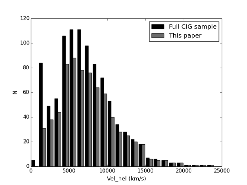
Figure 1: Distribution of radial velocities for the full CIG sample and our subset of 719 galaxies. This shows that both samples cover about the same redshift range (0.005 to 0.080), meaning that our capacity to separate details in the morphology of the galaxies will be roughly equivalent.

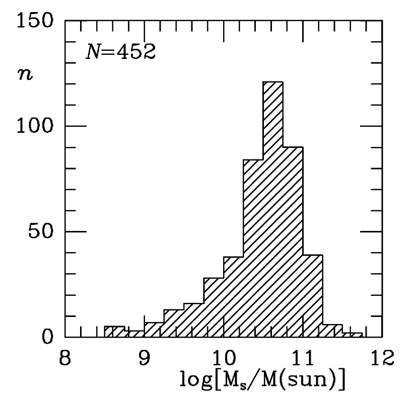
Figure 2: Distribution of stellar masses for 452 (63%) of our sample of 719 CIG galaxies. The mass estimates are from Fernández et al. (2013).

Table 1: Sample properties (Argudo-Hernández et al. 2013, 2015)

Parameter	Range
1	2
redshift	0.005 $<$ $z$ $<$ 0.080
$r$-band magnitude	11 $<$ $m_{r}$ $<$ 15.7
color index	0.2 $<$ $g-r$ $<$ 1.2
linear diameter	1.1 kpc $<$ $D$ $<$ 23.2 kpc
stellar mass	8.32 $<$ $log{M_{s}\over M_{\odot}}$ $<$ 11.42

3 CVRHS Morphology and Isolated Galaxies

In Buta et al. (2015), CVRHS morphology is described and applied to mid-infrared (3.6$\mu$m) images from the Spitzer Survey of Stellar Structure in Galaxies (S⁴G; Sheth et al. 2010). Although it was shown that the CVRHS system can be applied effectively in the mid-IR, the historical basis for the system is the $B$-band, the effective wavelength of which is only 0.44$\mu$m. Thus, to minimize systematic effects, it is best to use images obtained with a $B$-band filter or a filter close to the $B$-band. In the case of SDSS images, the filter closest to $B$ is the $g$-band at 0.477$\mu$m. We base our new classifications mainly on logarithmic, sky-subtracted $g$-band images in relative units of magnitudes per square arcsecond. This places the images in the “classification ready" mode of the de Vaucouleurs Atlas of Galaxies (Buta, Corwin, and Odewahn 2007=deVA). In principle, SDSS colour images can also be used for CVRHS classification, but these lack the dynamic range needed to see morphology in the bright centers of some galaxies and were not used for the classifications in this paper. Images in what the deVA refers to as “atlas units" have a broader dynamic range. The range used for the classifications from the AMIGA sample of images was approximately the same for all of the images. For calibrated SDSS $g$-band images, the range was 15.0-27.0 mag arcsec^-2.

The CVRHS system is a version of the de Vaucouleurs revised Hubble-Sandage (VRHS) system (de Vaucouleurs 1959) that takes into account more details of galaxy morphology that are of interest at the present time but at the same time preserves the main features of the original system. These details include lenses (Kormendy 1979), outer resonant subclass rings and pseudorings (Buta & Crocker 1991; Buta 1995, 2017b), ansae bars (Danby 1965; Martinez-Valpuesta et al. 2007; Buta 2012, 2013), nuclear rings (Burbidge & Burbidge 1960; Buta & Crocker 1993; Comerón et al. 2010), nuclear bars (de Vaucouleurs 1975; Buta & Crocker 1993; Erwin 2004), thick disks (Burstein 1979; Comeron et al. 2011), inclined (extraplanar) rings (Schweizer, Whitmore, and Rubin 1983), disky and boxy ellipticals (Kormendy & Bender 1996), spheroidal galaxies (Kormendy 2012), nuclear lenses (Buta & Combes 1996; Laurikainen et al. 2013), and barlenses (Laurikainen et al. 2013). Table 1 of Buta et al. (2015) summarizes all of the notation and features of CVRHS galaxy classification.

In addition to CVRHS classifications, we also present Arm Classes (ACs) for 514 of the 597 spiral galaxies in the sample, guided by Table 1 of Elmegreen & Elmegreen (1987). Arm Classes are based on symmetry and extent of the spiral arms in a galaxy, but can be uncertain or indeterminate when the inclination is high, as is the case for many of the 83 unclassified cases. Other reasons arm classes could only be estimated for 86% of the sample spiral galaxies are because either the stage is too early ($T\leq$ 0), the stage is too late ($T\geq$ 9), or the object is poorly resolved. Arm classes are useful in the context of the AMIGA sample because of the general view that spiral arms are a transient phenomenon requiring a “trigger," like a bar or a close companion (e.g., Kormendy & Norman 1979). Genuine examples of isolated grand design spirals would imply that strong spiral arms could nevertheless arise spontaneously within a disk without the presence of a major companion.

4 Procedure

Following Buta et al. (2015), the 719 AMIGA galaxies were classified from the prepared “classification ready" images by RB in two phases separated by more than 6 months. The main reason for this is to check the internal consistency of the full classifications. Table 2 includes the classifications from each phase, and Figure 3 shows comparisons of stage, family, and variety classifications between the two phases. In general, the agreement between the two phases is very good, and for the purposes of the remaining analysis, we take an unweighted average of the two phases using numerical indices listed in Table 3 of Buta et al. (2015). These unweighted average classifications are listed in Table 3.

Table 2: Phase 1 and 2 CVRHS Classifications for 719 AMIGA Galaxies. Col. 1: number in Karachentseva (1973) catalogue; col. 2: number in Principal Galaxy Catalogue (Paturel et al. 1989); col. 3: full phase 1 classification; col. 4: full phase 2 classification. (The full table will be made available online.)

Galaxy	PGC	Phase 1 type	Phase 2 type
1	2	3	4
$\rightarrow$ RA: 0h $\leftarrow$
CIG0001	205	SA(r$\underline{\rm s}$)bc	SA(rs)bc
CIG0002	223	SB(rs)cd	SB(rs)cd
CIG0004	279	SA(rs)c sp	SA(rs)c
CIG0005	602	SA(s)b:	SA(rs)b:
CIG0006	652	SAB(s)m/RG? pec	SB(s)m pec or Pec (merger)
CIG0007	793	SA$\underline{\rm B}$(rs)b	SAB(rs)ab
CIG0008	833	SA(s)cd	SA(s)cd
CIG0009	859	SA(s)d:	SAc pec
CIG0011	963	S$\underline{\rm A}$B(r$\underline{\rm s}$)d	SA(s)cd
CIG0012	1056	SAB(s)m sp pec	Sb: spw pec

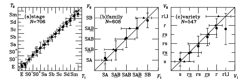
Figure 3: Comparison of Phase 1 and 2 classifications (Table 2) with respect to stage, family, and variety.

As in Buta et al. (2015), the averaging of two catalogues in this manner leads to extensive use of the de Vaucouleurs (1963) underline notation. This notation is meant to emphasize a particular part of a combined characteristic. For example, the family classification S$\underline{\rm A}$B implies a galaxy with only a trace of a bar; i.e., the galaxy is mostly nonbarred, while SA$\underline{\rm B}$ implies a galaxy with a clear but not strong bar, i. e., the galaxy is mostly barred. An inner variety of ($\underline{\rm r}$s) is a mostly closed inner pseudoring while an inner variety of (r$\underline{\rm s}$) is a mostly open inner pseudoring. The underline classifications for family and inner variety are well-enough defined to be applied directly, i.e., do not appear just because the final catalogue is an average of two phases. In principle, underline stages [like S$\underline{\rm a}$b (more Sa than Sb) or Sc$\underline{\rm d}$ (more Sd than Sc)] could also be applied directly. However, this is more difficult for stages, and underline stages only appear in average multi-phase classifications, mainly to preserve information.

Table 3: Mean CVRHS Classifications for 719 AMIGA Galaxies. Col. 1: number in Karachentseva (1973) catalogue; col. 2: number in Principal Galaxy Catalogue (Paturel et al. 1989); col. 3; mean numerical stage index; col. 4: Elmegreen arm class; col. 5: mean full classification; col. 6: notes (no abbreviations). (The full table will be made available online.)

Galaxy	PGC	$<T>$	AC	$<$Type$>$	notes
1	2	3	4	5	6
$\rightarrow$ RA: 0h $\leftarrow$
CIG0001	205	4.0	9	SA(rs)bc	UGC 5; excellent case
CIG0002	223	6.0	5	SB(rs)cd	UGC 12; excellent case
CIG0004	279	5.0	3	SA(rs)c sp	NGC 7817; excellent case;
NGC "	"00	"	"	00"	highly-inclined but not edge-on; like
NGC "	"00	"	"	00"	N0253; large (rs)
CIG0005	602	3.0	..	SA(r$\underline{\rm s}$)b:	CGCG 456-32; poorly resolved
CIG0006	652	9.0	4	SA$\underline{\rm B}$(s)m pec	NGC 9; resembles an RG, but no
NGC "	"00	"	"	00"	companion; $m$=1 spiral
CIG0007	793	2.5	9	SAB(rs)a$\underline{\rm b}$	CGCG 382-30; excellent face-on
NGC "	"00	"	"	00"	case; $m$=2 mainly
CIG0008	833	6.0	9	SA(s)cd	UGC 111; complex but regular
NGC "	"00	"	"	00"	spiral
CIG0009	859	6.0	1:	SA(s:)cd: pec	UGC 116; large blue associations
CIG0011	963	6.5	5	SA(s)c$\underline{\rm d}$	UGC 139; excellent, large
NGC "	"00	"	"	00"	late-type spiral
CIG0012	1056	6.0	..	SAB:(s:)cd: sp pec	UGC 149; pointy-ended; warping?

Table 4 shows that in general, the phase 1 and 2 classifications are very similar. Of the 719 galaxies, 112 (15.5%) received identical full classifications in the two phases, very similar to the 16% found by Buta et al. (2015). For stage, family, and variety, more than 50% of the subsets of the galaxies for which these aspects could be evaluated received identical classifications. However, for the outer variety, a significant fraction (36.8%) are in the category “$OV$ 1 no $OV$ 2, or $OV$ 2 no $OV$ 1," which includes all cases where an outer feature was recognized in one phase, but not in the other. It appears that more outer features were noticed in the first phase as compared with the second. Any recognition of an outer feature was included in the final adopted average classification.

Table 4: Comparison of Phase 1 and 2 classifications. Col. 1: “Type" = full letter classification [stage ($T$), family ($F$), inner variety ($IV$), and outer variety ($OV$)]. The categories “$IV$ 1 no $IV$ 2, or $IV$ 2 no $IV$ 1" and “$OV$ 1 no $OV$ 2, or $OV$ 2 no $OV$ 1" refer to those galaxies where a feature was recognized in one phase, but not in the other. Col. 2: numbers of galaxies in the categories listed in col. 1. Col. 3: percentages of these numbers out of the total numbers in the $T$, $F$, $IV$, and $OV$ subsamples.

Comparison	$n$	% of $N$
Type 1 = Type 2	112	15.5
$\Delta T$=0	429	60.5
$|\Delta T|$=1	224	31.6
$|\Delta T|$=2	35	4.9
$|\Delta T|>$2	21	3.0
$N$	709
$\Delta F$=0.00	448	73.4
$\Delta F$=0.25	116	19.0
$\Delta F$=0.50	43	7.1
$\Delta F$=0.75	1	0.2
$\Delta F$=1.00	2	0.3
$N$	610
$IV$ 1 = $IV$ 2	311	51.1
$IV$ 1 $\neq$ $IV$ 2	249	40.9
$IV$ 1 no $IV$ 2, or $IV$ 2 no $IV$ 1	49	8.0
$N$	609
$OV$ 1 = $OV$ 2	102	44.2
$OV$ 1 $\neq$ $OV$ 2	44	19.0
$OV$ 1 no $OV$ 2, or $OV$ 2 no $OV$ 1	85	36.8
$N$	231

The root mean square (rms) dispersion of classifications between phases 1 and 2 is calculated as

$$\sigma_{p1p2}(T)={1\over N}\Sigma(T_{p1}-T_{p2})^{2}$$

$$\sigma_{p1p2}(F)={1\over N}\Sigma(F_{p1}-F_{p2})^{2}$$

$$\sigma_{p1p2}(IV)={1\over N}\Sigma(IV_{p1}-IV_{p2})^{2}$$

where $N$ is the total number of galaxies in each comparison. From the comparisons shown in Figure 3, and using the numerical codes from Buta et al. (2015), we obtain $\sigma_{p1p2}(T)$ = 0.89 stage intervals, corresponding to $\sigma_{p1}(T)\approx\sigma_{p2}(T)$ = 0.63 stage intervals, based on 707 galaxies. Here 1 stage interval means a difference like Sbc to Sc, or S0/a to Sa, so the internal consistency is good to better than 1 stage interval. For family, we find $\sigma_{p1p2}(F)$ = 0.72 family intervals, where 1 family interval equals a difference like SA to S$\underline{\rm A}$B or SA$\underline{\rm B}$ to SB. This corresponds to $\sigma_{p1}(F)\approx\sigma_{p2}(F)$ = 0.51 family intervals, based on 608 galaxies.

For inner varieties, we obtain $\sigma_{p1p2}(IV)$ = 1.16 variety intervals, where 1 variety interval equals a difference like (r) to ($\underline{\rm r}$s) or (r$\underline{\rm s}$) to (s). This corresponds to $\sigma_{p1}(IV)\approx\sigma_{p2}(IV)$ = 0.82 variety intervals, based on 547 galaxies. The consistency is somewhat poorer for inner variety because of the many additional categories added by the recognition of inner ring-lenses (rl) and inner lenses (l), which are combined in Figure 3.

5 External Comparison of Classifications

Galaxy classification at the present time is often done by consensus and does not always involve estimation of standard types in the fashion Sa, SBb, SAB(rs)ab, etc. For example, Fukugita et al. (2007) classified 2253 SDSS galaxies in a modified Hubble system, based on the independent examination of all of the sample galaxies by three astronomers. In this study, only stages and families were judged; inner, outer, and nuclear varieties were not. Ann, Seo, and Ha (2015) estimated stages and families of 5836 galaxies having $z$ $<$ 0.01. Baillard et al. (2011) present classifications for 4458 galaxies in the EFIGI sample, based on the participation of 10 professional astronomers who each classified a 10% subset of the sample, including an overlap sample to examine and remove personal equations and potential biases. In this case, the classifications were carried out using numerical codings of 16 “attributes," or morphological characteristics.

Kartaltepe et al. (2016) used a similar procedure to classify 7634 galaxies that are part of the CANDELS survey, a dataset that includes deep images of galaxies in the redshift range 0 $<$ $z$ $<$ 4. In this case, 65 astronomers contributed to the final classifications, which were tailored for the higher redshift part of the sample (i.e., did not involve classifications like SB(rs)c, SA(s)a, etc.)

We have not used the multi-classifier approach in our examination of the AMIGA sample. To evaluate the external consistency of our classifications, we compare our $T$ and $F$ estimates with those from five other sources: Baillard et al. (2011); the Nair & Abraham (2010) sample (14034 SDSS galaxies); Fernàndez-Lorenzo et al. (2012; all CIG galaxies); Durbala et al. (2008; 101 AMIGA galaxies from SDSS); and RC3. Figures 4 and  5 show comparisons between our Table 3 mean phase 1 and 2 classifications and the galaxies in common with these other sources for stage and family, respectively. These show no serious scale differences between sources, but the large amount of scatter is consistent with previous findings. Similar to equations 1, we estimate the root mean square (rms) dispersion between observers $i$ and $j$ as

$$\sigma_{ij}^{2}={1\over N}\Sigma(T_{i}-T_{j})^{2}$$

where again $N$ is the total number of galaxies in the comparison. If we assume no systematic effects between different observers, then these rms dispersions are related to the individual dispersions through equations like

$$\sigma_{ij}^{2}=\sigma_{i}^{2}+\sigma_{j}^{2}$$

This will give 15 equations in 6 unknowns which we solve using linear least squares.

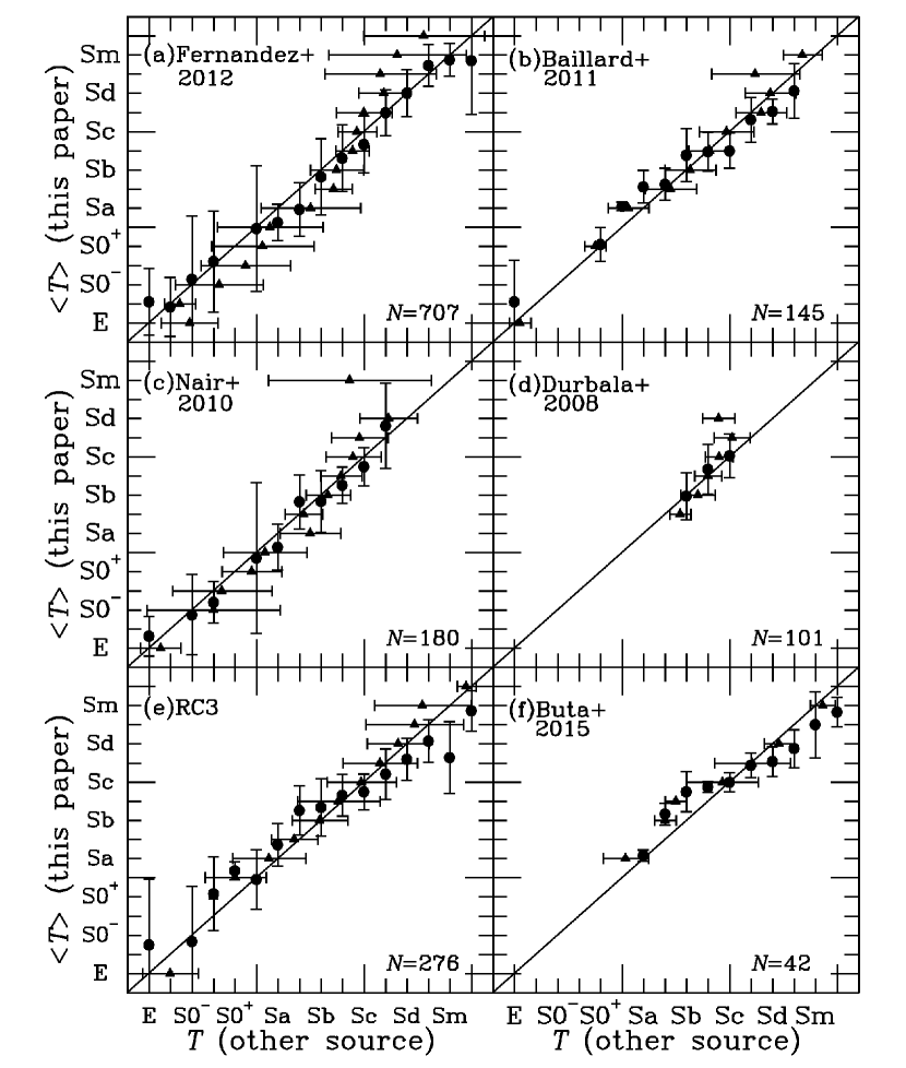
Figure 4: Comparison of Table 3 mean Phase 1 and 2 stages with similar data from six other sources: (a) Fernández-Lorenzo et al. (2012); (b) Baillard et al. (2011); (c) Nair & Abraham (2010); (d) Durbala et al. (2008); (e) RC3 (de Vaucouleurs et al. 1991); and (f) Buta et al. (2015).

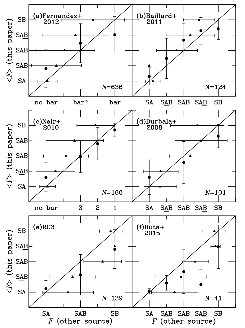
Figure 5: Comparison of Table 3 mean Phase 1 and 2 families with similar data from six other sources: (a) Fernández-Lorenzo et al. 2012; (b) Baillard et al. (2011); (c) Nair & Abraham (2010); (d) Durbala et al. (2008); (e) RC3 (de Vaucouleurs et al. 1991); and (f) Buta et al. (2015).

Table 5 summarizes the results of these comparisons. The $\sigma_{i}$ on stages range from 0.6 to 1.3 stage intervals and can only be considered approximate because each $\sigma_{ij}$ combination involves a different subset of the sample, with the number of galaxies ranging from $N$ = 39 to $N$ = 705. The same is also true for family classifications. The average external consistency on stages is $<\sigma(T)>$ $\approx$ 1.1 stage intervals, while the external consistency on family classifications is 0.24 or $\approx$1 family interval.

Table 5: External Agreement Between Classifications. Each column gives the rms dispersion between the two sources ($i$ and $j$) indicated. The number in parentheses next to each value is the number of galaxies in each comparison. The individual $\sigma_{i}$ are derived from a linear least squares analysis. Sources: EFIGI=Baillard et al. (2011); NA2010=Nair & Abraham (2010); Fern2012=Fernández-Lorenzo et al. (2012); Durb2008=Durbala et al. (2008); RC3=de Vaucouleurs et al. (1991).

Source	$j$	RB	EFIGI	NA2010	Sul2006	Durb2008	RC3
				(a) $\sigma_{ij}$ Stage
$i$		1	2	3	4	5	6
EFIGI	2	1.27(145)	……….	……….	……….	……….	……….
NA2010	3	1.61(180)	1.44( 57)	……….	……….	……….	……….
Fern2012	4	1.83(705)	1.38(147)	1.89(182)	……….	……….	……….
Durb2008	5	1.21(101)	1.31( 49)	1.52( 39)	1.10(101)	……….	……….
RC3	6	1.62(276)	1.84(147)	1.57( 60)	1.83(280)	1.39( 55)	……….
$\sigma_{i}(T)$		1.06	0.95	1.21	1.25	0.62	1.29
				(b) $\sigma_{ij}$ Family
EFIGI	2	0.24(124)	……….	……….	……….	……….	……….
NA2010	3	0.29(161)	0.20( 54)	……….	……….	……….	……….
Sul2006	4	0.36(637)	0.29(131)	0.31(176)	……….	……….	……….
Durb2008	5	0.32(101)	0.30( 49)	0.35( 39)	0.38(101)	……….	……….
RC3	6	0.39(149)	0.43( 82)	0.38( 32)	0.54(149)	0.44( 48)	……….
$\sigma_{i}(F)$		0.19	0.14	0.16	0.30	0.25	0.38

Naim et al. (1995) carried out an experiment to examine the external consistency in morphological classifications between different observers. Using paper copies of blue-light images (or monitor displays) of 831 galaxies, six observers classified the galaxies in modified Hubble systems. Although general consistency in stage classifications between observers was found, a non-negligible scatter was also found with an average $\sigma_{ij}$ $\approx$ 1.8 stage intervals. Our analysis in Table 5 has a $<\sigma_{ij}>$ =1.52, which may be a little better because of improved image quality.

In general, $\sigma(T)$ = 1.1 can be considered “good" for Hubble classifications from different sources. It means that a galaxy classified as type Sbc from one source could be classified as Sb or Sc by another source. This level of disagreement is relatively small compared to the 16-stage extent of the VRHS sequence.

6 Morphological Characteristics of the Sample

6.1 Stages

Table 6 lists our revised classification results, which are plotted as histograms in Figure 6. The distributions of stages, families, inner varieties, outer varieties and Elmegreen arm classes are compiled for two samples: the full set of AMIGA galaxies classified, and a subset restricted to more face-on disks (inclination $i$ $\leq$ 60^o). The latter restriction is important because features such as bars and rings can become harder to recognize when the inclination is high.

The distribution of stages confirms the finding of Sulentic et al. (2006; see also Fernández-Lorenzo et al. 2012) that the most abundant types among isolated galaxies are Sb-Sc spirals. However, while these constitute 63% of the Sulentic et al. (2006) sample and 68% of the Fernández-Lorenzo et al. (2012) sample, they make up 47%-50% of our current sample. We also find Sa-Sd spirals at the 75% level, compared to 82% for Sulentic et al. (2006). For E and S0 galaxies, we find 13.9% for the full sample and 16.3% for the inclination-restricted subset, both comparable to what was found by Sulentic et al. (2006). The higher value for the restricted subset is partly or perhaps wholly due to the rejection of spindle galaxies. In general, the results from the restricted subset are very similar to those from the full sample.

Sulentic et al. (2006) noted a low fraction of Sa galaxies in their sample. Including S0/a types, their classification has 3.2% early-type spirals compared to 10.3%-10.7% in our classification. In their sample also, Sdm-Im types make up 5.6% of the galaxies, while these make up 7.5%-2.5% of our sample. Considering the full range of types from S0/a to Sm, spirals represent 84.2%-82.3% of our AMIGA sample.

Of the 706 galaxies in the sample for which a stage could be judged, 18% have a CVRHS classification in Table 3 with the appendage “pec," implying something “peculiar" or unusual, most likely an asymmetry. For some objects, the classification is “Pec (merger)", meaning the object could be a merger of two galaxies. Although it is tempting to conclude that such cases must therefore not be truly isolated, the presence of peculiarities is not an automatic disqualifier from our catalogue. This is because isolation only depends on neighborhood, and we can ask if some peculiarities could arise in isolation. Objects classified as “Pec (merger)" are by default not included in Table 6 since they have no stage, family, inner variety, or outer variety as part of their classification.

Eleven sample objects (CIG 31, 424, 468, 532, 533, 678, 773, 893, 927, and 1038) have apparent close companions. Without redshift information for many of the galaxies, and without perturbations pointing straight to the potential companion, we cannot affirm that most of these cases involve real companions. An exception is CIG 533, for which redshift information is available for both the galaxy and the companion.

Table 6: Histogram Data for Morphological Analysis. The full sample includes all the galaxies in the AMIGA sample that were classifiable into the given categories. The restricted subset excludes galaxies having an inclination $i$ $>$ 60^o.

Stage	% ($n$)	Family	% ($n$)	Outer	% ($n$)	Arm	% ($n$)
		Variety		Feature		Class
Full sample
E	4.0 ( 28)	SA	51.6 (331)	(R′)	52.8 (121)	AC 1	2.5 ( 13)
E+	1.3 ( 9)	S$\underline{\rm A}$B	5.1 ( 33)	(R)	4.4 ( 10)	AC 2	2.5 ( 13)
S0-	2.7 ( 19)	SAB	23.2 (149)	(RL)	4.8 ( 11)	AC 3	7.6 ( 39)
S0o	2.0 ( 14)	SA$\underline{\rm B}$	4.2 ( 27)	(R′L)	8.3 ( 19)	AC 4	8.6 ( 44)
S0+	4.0 ( 28)	SB	15.9 (102)	(L)	4.4 ( 10)	AC 5	12.6 ( 65)
S0/a	3.4 ( 24)	S$\underline{\rm{A}}$B+SAB+SA$\underline{\rm{B}}$+SB	48.4 (311)	(R1)	1.7 ( 4)	AC 6	8.6 ( 44)
Sa	6.8 ( 48)	$N$	642	(R1L)	0.4 ( 1)	AC 7	3.9 ( 20)
Sab	6.1 ( 43)	…….	…….	(R${}_{1}^{\prime}$)	14.0 ( 32)	AC 8	15.4 ( 79)
Sb	14.2 (100)	(s)	41.6 (251)	(R${}_{2}^{\prime}$)	7.0 ( 16)	AC 9	28.0 (144)
Sbc	14.4 (102)	(r$\underline{\rm s}$)	8.6 ( 52)	(R1R${}_{2}^{\prime}$)	2.2 ( 5)	AC 12	10.3 ( 53)
Sc	18.7 (132)	(rs)	24.5 (148)	R1+R2	25.3 ( 58)	AC1-AC4	21.2 (109)
Scd	8.9 ( 63)	($\underline{\rm r}$s)+(r′l)	9.4 ( 57)	$N$	229	AC5-AC8	40.5 (208)
Sd	6.1 ( 43)	(r)	7.9 ( 48)	…….	…….	AC9,AC12	38.3 (197)
Sdm	3.0 ( 21)	($\underline{\rm r}$l)	1.8 ( 11)	…….	…….	$N$	514
Sm	2.5 ( 18)	(rl)	2.0 ( 12)	…….	…….	…….	…….
Im	2.0 ( 14)	(r$\underline{\rm l}$)	0.7 ( 4)	…….	…….	…….	…….
E-S0+	13.9 ( 98)	(l)	3.5 ( 21)	…….	…….	…….	…….
Sa-Sd	75.2 (531)	(r$\underline{\rm{s}}$)+(rs)+($\underline{\rm{r}}$s)+(r′l)+(r)	50.5 (305)	…….	…….	…….	…….
Sb-Sc	47.3 (334)	($\underline{\rm{r}}$l)+(rl)+(r$\underline{\rm{l}}$)+(l)	7.9 ( 48)	…….	…….	…….	…….
$N$	706	$N$	604	…….	…….	…….	…….
Restricted to $i\leq$60o
E	6.3 ( 28)	SA	50.1 (203)	(R′)	51.4 ( 75)	AC 1	2.3 ( 8)
E+	2.0 ( 9)	S$\underline{\rm A}$B	5.2 ( 21)	(R)	4.8 ( 7)	AC 2	1.2 ( 4)
S0-	2.7 ( 12)	SAB	24.7 (100)	(RL)	4.1 ( 6)	AC 3	5.3 ( 18)
S0o	1.6 ( 7)	SA$\underline{\rm B}$	3.0 ( 12)	(R′L)	8.2 ( 12)	AC 4	5.6 ( 19)
S0+	3.6 ( 16)	SB	17.0 ( 69)	(L)	4.8 ( 7)	AC 5	12.0 ( 41)
S0/a	3.4 ( 15)	S$\underline{\rm{A}}$B+SAB+SA$\underline{\rm{B}}$+SB	49.9 (202)	(R1)	2.7 ( 4)	AC 6	9.4 ( 32)
Sa	7.3 ( 32)	$N$	405	(R1L)	0.7 ( 1)	AC 7	2.9 ( 10)
Sab	6.6 ( 29)	…….	…….	(R${}_{1}^{\prime}$)	11.0 ( 16)	AC 8	16.1 ( 55)
Sb	13.8 ( 61)	(s)	35.3 (137)	(R${}_{2}^{\prime}$)	9.6 ( 14)	AC 9	32.6 (111)
Sbc	16.8 ( 74)	(r$\underline{\rm s}$)	9.0 ( 35)	(R1R${}_{2}^{\prime}$)	2.7 ( 4)	AC 12	12.6 ( 43)
Sc	19.7 ( 87)	(rs)	28.1 (109)	R1+R2	26.7 ( 39)	AC1-AC4	14.4 ( 49)
Scd	7.3 ( 32)	($\underline{\rm r}$s)+(r′l)	10.8 ( 42)	$N$	146	AC5-AC8	40.5 (138)
Sd	3.6 ( 16)	(r)	8.5 ( 33)	…….	…….	AC9,AC12	45.2 (154)
Sdm	2.7 ( 12)	($\underline{\rm r}$l)	2.1 ( 8)	…….	…….	$N$	341
Sm	1.1 ( 5)	(rl)	1.5 ( 6)	…….	…….	…….	…….
Im	1.4 ( 6)	(r$\underline{\rm l}$)	0.5 ( 2)	…….	…….	…….	…….
E-S0+	16.3 ( 72)	(l)	4.1 ( 16)	…….	…….	…….	…….
Sa-Sd	75.1 (331)	(r$\underline{\rm{s}}$)+(rs)+($\underline{\rm{r}}$s)+(r′l)+(r)	56.4 (219)	…….	…….	…….	…….
Sb-Sc	50.3 (222)	($\underline{\rm{r}}$l)+(rl)+(r$\underline{\rm{l}}$)+(l)	8.2 ( 32)	…….	…….	…….	…….
$N$	441	$N$	388	…….	…….	…….	…….

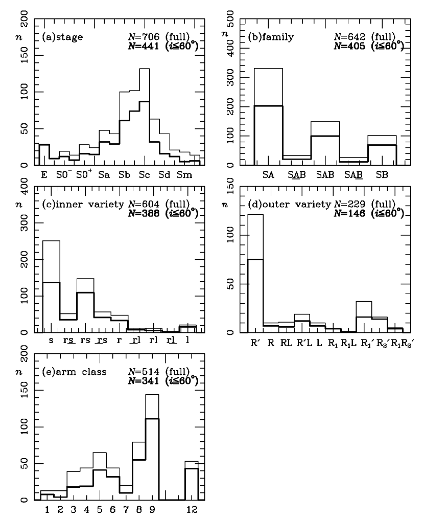
Figure 6: Histograms of morphological classifications from Table 6 for the full sample (light solid histogram) and a subsample restricted to inclinations $i$ less than or equal to 60^o (heavy solid histogram). The numbers of objects $N$ in each sample are indicated.

The distribution of stages for the AMIGA sample is very different from that for the S⁴G sample. Figure 5 of Buta et al. (2015) shows that the latter sample strongly emphasizes extreme late-type disk galaxies, i.e., galaxies in the stage range Sd-Im. These constitute 48.5%$\pm$1.4% of 1240 low inclination galaxies in the S⁴G sample, compared to 16.1%$\pm$1.8% for the restricted subset of AMIGA galaxies.

6.2 Bar Classifications and Fraction

The bar fraction for isolated galaxies is clearly of interest. Verley et al. (2007c) observed a sample of 45 well-resolved, low inclination CIG galaxies and found that 60% are barred and 33% are nonbarred. Here we define the bar fraction in two ways: (1) $f_{1bar}$ = $100*[N-n({\rm SA})-n({\rm S}\underline{\rm A}{\rm B})]/N$, where $N$ is the total number of galaxies classifiable as to family, $n$(SA) = number of SA galaxies, and $n$(S$\underline{\rm{A}}$B) = number of S$\underline{\rm{A}}$B galaxies. This is how the bar fraction was defined by Buta et al. (2015). (2) $f_{2bar}$ = $100*[N-n(SA)]/N$ - This definiton allows for a fairer comparison with $f_{bar}$ in the mid-IR. Bars tend to generally look stronger in IR light (the “stronger bar effect"), and this definition assumes that an S$\underline{\rm{A}}$B galaxy in the $g$-band might be classified as SAB in the mid-IR. This allows the bar fraction to include both the strongest and the weakest-looking bars. With these definitions and the data in Table 6, the bar fraction is $f_{1bar}$ = 45%$\pm$3% and $f_{2bar}$=50.0%$\pm$3%, both for the restricted (low inclination) subset. These values are lower than the 62%-71% found by Buta et al. (2015) for the S⁴G mid-infrared sample, and for the Ohio State University Bright Galaxy Survey (Eskridge et al. 2000). These percentages are over all types. As shown in Figure 7 of Buta et al. (2015), the bar fraction has a minimum of $\approx$40% in the stage range S$\underline{\rm b}$c-Sc, the same range where the bulk of isolated spirals are found. The equivalent version of Figure 7 of Buta et al. (2015) for the full AMIGA sample and its inclination-restricted subset is shown in Figures 7a and b, respectively. As for the S⁴G sample, our AMIGA sample shows a minimum bar fraction in the stage range Sbc-Sc, ranging from 37%$\pm$5% at stage Sbc to 26%$\pm$4% at stage Sc. These numbers change to 38%$\pm$6% and 29%$\pm$5% for the restricted subset. Only 16% of our AMIGA galaxies were classified as family “SB" in the full sample and 17% in the restricted subset.

Table 7 summarizes the bar fraction of AMIGA galaxies over the same ranges of type as in Table 7 of Buta et al. (2015). If we compare the restricted AMIGA sample to the equivalent S⁴G subset (infrared axis ratio $q_{25.5}$$\leq$0.5), for stages S0/a to Sc, the result is $f_{1bar}$ = 40%$\pm$3% for AMIGA galaxies versus 55%$\pm$2% for S⁴G galaxies. For stages Scd to Sm, the fractions are both higher: $f_{1bar}$ = 66%$\pm$6% for AMIGA versus 81%$\pm$2% for S⁴G. The bar fraction of AMIGA galaxies appears to be significantly lower than in S⁴G galaxies; however, especially for the S0/a-Sc stage range, the difference could be partly attributable to the “stronger bar" effect in mid-IR images. Thus, $f_{2bar}$ is probably a better definition for $g$-band classifications. Table 7 shows that $f_{2bar}$ = 46%$\pm$3% for S0/a to Sc and 72%$\pm$6% for Scd-Sm. Even allowing for the different definitions of $f_{bar}$, the AMIGA sample has a slightly lower bar fraction than does the S⁴G sample.

Over the full type range of S0/a to Sm, a more significant difference emerges: $f_{2bar}$ = 50%$\pm$3% for AMIGA galaxies versus $f_{1bar}$ = 66%$\pm$2% for S⁴G galaxies. Much of this difference is attributable to the emphasis of the AMIGA sample on Sb-Sc galaxies, as compared to Scd-Im galaxies in S⁴G. The latter range pulls up the bar fraction in the mid-IR substantially.

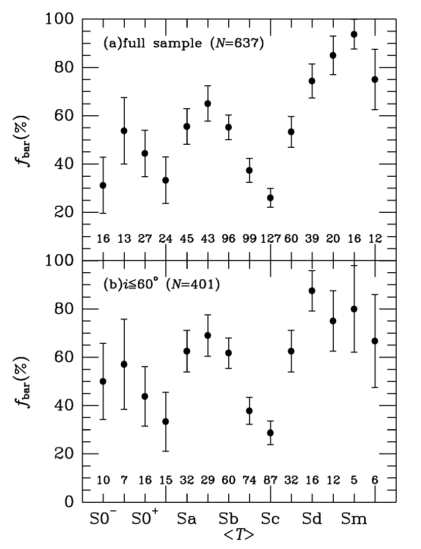
Figure 7: Graphs of the bar fraction $f_{bar}$ versus the mean phase 1 and 2 stage along the CVRHS Hubble sequence: (a) for the full sample unrestricted by inclination, and (b) for the restricted subset of galaxies having $i$ less than or equal to 60^o. The number of objects $n$ at each stage is indicated.

Figures 3– 5 show that, while our Phase 1 and 2 bar classifications are internally consistent, systematic disagreements with other sources of bar classifications are present. In comparison with RC3 classifications, there is a trend for weaker bar classifications in Table 3. Compared to Baillard et al. (2011) and Nair & Abraham (2010), however, there is a slight trend for stronger bar classifications in Table 3. Fernández-Lorenzo et al. (2012) were able to classify bars only as being “bar", “bar?", and “no bar", which we have treated as SB, SAB, and SA, respectively. For these we find reasonably good agreement (Figure 5a).

The graphs in Figures 4f and  5f show the comparisons between Table 3 types and those based on mid-IR images from Buta et al. (2015). Only 42 galaxies are in common between the S⁴G sample and our AMIGA sample. The comparisons show both an “earlier effect" and a “stronger bar effect" between the 3.6$\mu$m classifications and our Table 3 $g$-band classifications, which is not unexpected.

6.3 Inner and Outer Varieties

The results for inner variety ($IV$) classifications in Table 6 show that the dominant variety is (s), which is also characteristic of the S⁴G sample. Figure 8 shows the relative frequency of the non-(s) varieties versus the mean phase 1 and 2 stage. As in Figure 8 of Buta et al. (2015), this frequency is highest among early-type disk galaxies and lowest among the very latest types. Table 7 summarizes the frequencies for different ranges of stage and feature types. For the stage range S0/a to Sc, the restricted AMIGA subset has $f_{IV}$ = 54%$\pm$3% for (rs)+($\underline{\rm r}$s)+(r^′l)+(r) versus 51%$\pm$2% for the same types for S⁴G (Table 8 of Buta et al. 2015). For Scd-Sm, the numbers are $f_{IV}$ = 23%$\pm$5% versus 13%$\pm$2%, respectively. Thus, the AMIGA sample has a slightly higher percentage of rings and pseudorings compared to S⁴G. As for the bar fraction, the difference is more significant when the full type range (S0/a-Sm) is considered: 49%$\pm$3% for AMIGA versus 34%$\pm$2$ for S⁴G. Again, this is largely due to the strong emphasis of the S⁴G sample on later type galaxies as compared to the AMIGA sample.

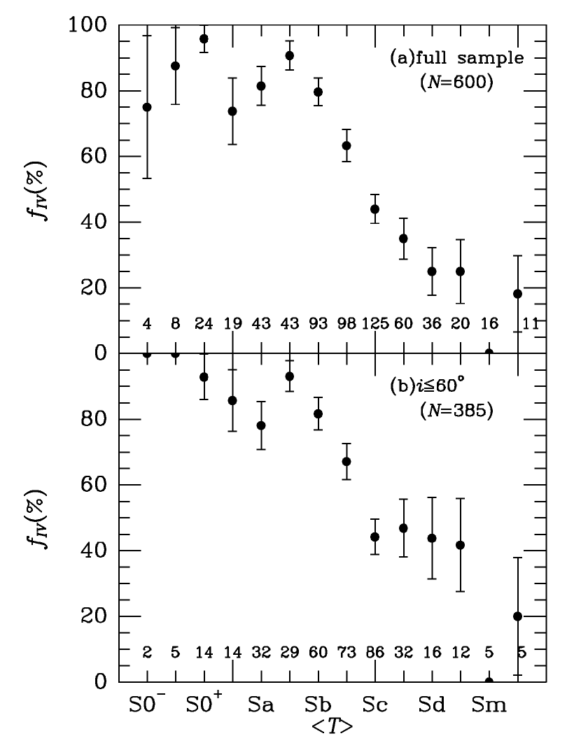
Figure 8: Graphs of the inner ring/pseudoring/lens fraction $f_{IV}$ versus the mean phase 1 and 2 stage along the CVRHS Hubble sequence: (a) for the full sample unrestricted by inclination, and (b) for the restricted subset of galaxies having $i$ less than or equal to 60^o. The number of objects $n$ at each stage is indicated.

Table 7: Relative frequencies of bars and inner rings in the AMIGA sample, in intervals of stage.

Parameter	Features	S0-–S0+	S0/a–Sc	Scd-Sm	S0/a-Sm
$f_{bar}$% (full)	SAB+SA$\underline{\rm{B}}$+SB	37.5$\pm$ 6.5( 21)	37.1$\pm$ 2.3(161)	64.4$\pm$ 4.1( 87)	43.6$\pm$ 2.1(248)
$f_{bar}$% (full)	S$\underline{\rm{A}}$B+SAB+SA$\underline{\rm{B}}$+SB	42.9$\pm$ 6.6( 24)	42.4$\pm$ 2.4(184)	68.9$\pm$ 4.0( 93)	48.7$\pm$ 2.1(277)
$N$		56	434	135	569
$f_{bar}$% ($i$$\leq$60o)	SAB+SA$\underline{\rm{B}}$+SB	47.1$\pm$ 8.6( 16)	39.7$\pm$ 2.8(118)	66.2$\pm$ 5.9( 43)	44.5$\pm$ 2.6(161)
$f_{bar}$% ($i$$\leq$60o)	S$\underline{\rm{A}}$B+SAB+SA$\underline{\rm{B}}$+SB	47.1$\pm$ 8.6( 16)	45.5$\pm$ 2.9(135)	72.3$\pm$ 5.6( 47)	50.3$\pm$ 2.6(182)
$N$		34	297	65	362
$f_{IV}$% (full)	rs+$\underline{\rm r}$s+r′l+r	38.9$\pm$ 8.1( 14)	51.8$\pm$ 2.4(218)	14.4$\pm$ 3.1( 19)	42.9$\pm$ 2.1(237)
$f_{IV}$% (full)	$\underline{\rm r}$l+rl+r$\underline{\rm l}$+l	52.8$\pm$ 8.3( 19)	5.9$\pm$ 1.2( 25)	0.8$\pm$ 0.8( 1)	4.7$\pm$ 0.9( 26)
$N$		36	421	132	553
$f_{IV}$% ($i$$\leq$60o)	rs+$\underline{\rm r}$s+r′l+r	42.9$\pm$10.8( 9)	54.1$\pm$ 2.9(159)	23.1$\pm$ 5.2( 15)	48.5$\pm$ 2.6(174)
$f_{IV}$% ($i$$\leq$60o)	$\underline{\rm r}$l+rl+r$\underline{\rm l}$+l	52.4$\pm$10.9( 11)	5.8$\pm$ 1.4( 17)	1.5$\pm$ 1.5( 1)	5.0$\pm$ 1.2( 18)
$N$		21	294	65	359

The most common outer variety classification in Table 3 is no outer feature recognized. Among those cases where an outer feature is recognized (229 in the full sample, and 146 in the restricted subset), the most common type of feature is an outer pseudoring, R^′. These are made of outer arms whose variable pitch angle leads to a ring-like pattern. Combined with outer pseudoring-lenses, R^′L, these features are found in 56%$\pm$4% of the restricted AMIGA subset as compared to 53%$\pm$3% for the same features in the S⁴G low inclination subset. In comparison, closed outer rings (R) are rare in our sample. This is easily explained by the distribution of stages: the emphasis of our sample on intermediate-to-late-type spirals favours outer pseudorings over closed outer rings (e.g., see also Buta & Combes 1996).

Other kinds of outer features are also seen in AMIGA galaxies, including what Buta & Crocker (1991) and Buta (1995) called the outer Lindblad resonance subclasses R₁, R${}_{1}^{\prime}$, R${}_{2}^{\prime}$, and R₁R${}_{2}^{\prime}$ (now called “outer resonant subclasses"; Buta 2017). In the full sample there are 58 cases, while in the restricted subset there are 39; these correspond to 25% and 27%, respectively, of those samples. In contrast, these features were found in 10%$\pm$2% of 283 S⁴G galaxies classified as having an outer feature. The closed outer ring (R), outer ring-lens (RL), outer pseudoring-lens (R^′L), and outer lens (L) galaxies constitute 14%$\pm$2% of the full sample and 14%$\pm$3% of the restricted subset. Pseudorings are still the most common features even among these categories: R${}_{1}^{\prime}$ for the outer resonant classes and R^′L for the outer ring-lens classes.

6.4 Arm Classes

The distribution of arm classes shows that grand design spirals (AC8, AC9, AC12) occur in 53.7% of the classifiable full sample cases and 61.3% of the classifiable restricted subset cases. In contrast, flocculent spirals (AC1-4) occur in 20.2% of the full sample cases, and 14.4% of the restricted subset. Figure 9 shows six of the grand design cases. One case, CIG 86, has a strong bar that could drive its grand-design pattern (Kormendy and Norman 1979). The other five, however, are mostly nonbarred, and in fact 50% of the 276 AC 8, 9, and 12 galaxies in the full sample are nonbarred. While all six of the galaxies in Figure 9 have no significant companions, four do have small companions (not in the field covered by the images) ranging from $\approx$1 galaxy diameter away (CIG 304, 313, 630) to more than 5 diameters for CIG 333. CIG 281 has no similar small companions. Most if not all of the “knots" seen in these images are likely star forming regions or foreground stars rather than companion galaxies. The high abundance of grand design, nonbarred spirals in the AMIGA sample is an important observation, because it favours the possibility that such spirals have arisen purely from internal effects, rather than external interactions.

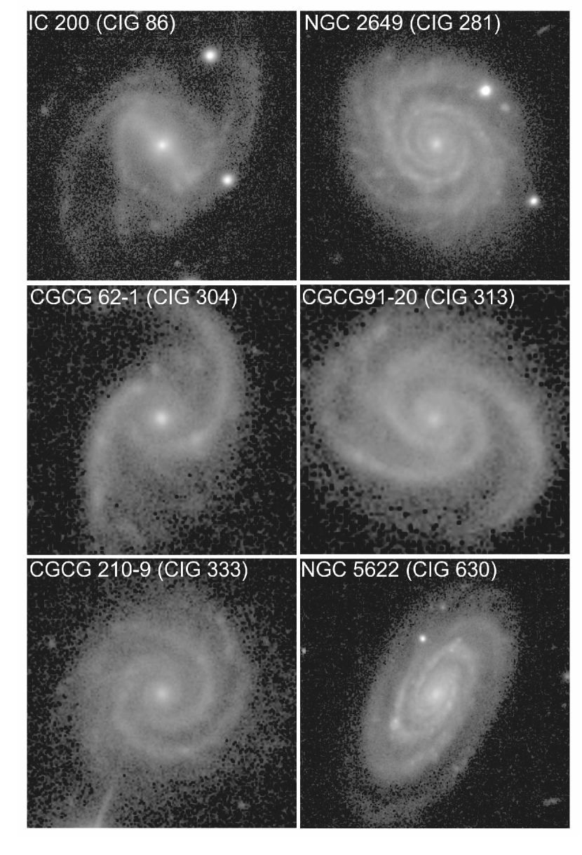
Figure 9: Six grand design spirals (CIG 86, 281, 304, 313, 333, 630) from the AMIGA sample.

Table 8: Morphology and stellar mass in isolated galaxies. Col. 1: range of specific morphological types or characteristics; col. 2: average log stellar mass in units of solar masses; col. 3: standard deviation of mean log stellar mass; col 4: mean stage of subset; col. 5: standard deviation of mean stage; col. 6: number of galaxies in subset.

Morphology range	$<log{M_{s}\over M_{\odot}}>$	$\sigma_{1}$	$<T>$	$\sigma_{1}$	$n$
1	2	3	4	5	6
Full sample
E–S0+	10.72	0.36	-3.0	1.5	54
S$\underline{\rm 0}$/a–Sab	10.72	0.30	1.1	0.7	81
Sa$\underline{\rm b}$–Sc	10.58	0.32	4.0	0.8	220
S$\underline{\rm c}$d–Im	9.80	0.55	7.1	1.4	89
SA	10.52	0.45	3.8	7.1	209
S$\underline{\rm{A}}$B,SAB,SA$\underline{\rm{B}}$	10.42	0.52	3.7	2.7	139
SB	10.31	0.65	4.2	3.2	61
s,r$\underline{\rm s}$	10.27	0.55	5.0	2.2	195
rs	10.57	0.38	3.6	1.6	94
$\underline{\rm r}$s,r	10.72	0.32	1.9	1.7	69
$\underline{\rm r}$l,rl,r$\underline{\rm l}$,l	10.75	0.30	0.1	2.5	28
(R′)	10.53	0.52	3.6	2.0	73
R,RL,R′L,L	10.67	0.44	1.0	2.6	35
R1,R1L,R${}_{1}^{\prime}$,R${}_{2}^{\prime}$,R1R${}_{2}^{\prime}$	10.74	0.18	1.8	1.2	35
AC 1–4	10.13	0.59	5.7	1.9	61
AC 5–7	10.40	0.40	4.6	1.4	84
AC 8,9,12	10.63	0.34	3.4	1.4	179
Restricted to $i$$\leq$60o
E–S0+	10.75	0.33	-3.0	1.5	31
S$\underline{\rm 0}$/a–Sab	10.75	0.30	1.1	0.7	48
Sa$\underline{\rm b}$–Sc	10.60	0.31	4.0	0.8	146
S$\underline{\rm c}$d–Im	9.84	0.50	6.9	1.4	37
SA	10.55	0.46	3.5	2.4	120
S$\underline{\rm{A}}$B,SAB,SA$\underline{\rm{B}}$	10.50	0.42	3.3	2.4	89
SB	10.50	0.46	3.4	3.0	40
s,r$\underline{\rm s}$	10.36	0.50	4.7	1.9	105
rs	10.55	0.38	3.5	1.6	72
$\underline{\rm r}$s,r	10.77	0.27	2.0	1.8	46
$\underline{\rm r}$l,rl,r$\underline{\rm l}$,l	10.73	0.33	0.3	2.7	19
(R′)	10.56	0.47	3.3	2.0	45
R,RL,R′L,L	10.74	0.37	1.1	2.1	22
R1,R1L,R${}_{1}^{\prime}$,R${}_{2}^{\prime}$,R1R${}_{2}^{\prime}$	10.76	0.19	1.9	1.3	22
AC 1–4	10.10	0.53	5.6	1.8	26
AC 5–7	10.42	0.33	4.6	1.3	51
AC 8,9,12	10.64	0.34	3.3	1.4	137

7 Morphology and Stellar Mass

Table 8 summarizes the average stellar masses of the isolated galaxies in our sample for which a mass estimate is available, for the full samples and for the subsets restricted to $i$ $\leq$ 60^o. Because we have mass estimates for only about 60% of our sample (Figure 2), the log masses are averaged over a range of types or morphological characteristics. The table highlights some definite but not unexpected trends which are shown in Figure 10. First, the early stages (E to Sab; Figure 10a) are considerably more massive than the later stages (S$\underline{\rm c}$d–Im), by a factor of nearly 8. The intermediate stages (Sa$\underline{\rm b}$–Sc) are intermediate in log mass but closer to the early types on average than the later types. Second, the average log mass of the nonbarred (SA) galaxies in the sample is slightly higher than that of the barred (SAB and SB) galaxies (Figure 10b), although the effect is smaller for the restricted subsets.

Among inner varieties, the isolated galaxies of types (s) and (r$\underline{\rm s}$) are less massive than those of types $\underline{\rm r}$s) and (r) by a factor of nearly 3, with (rs) galaxies intermediate (Figure 10c). Galaxies of types ($\underline{\rm r}$l), (rl), (r$\underline{\rm l}$), and (l) have stellar masses comparable to those of types ($\underline{\rm r}$s), and (r). Among outer varieties, isolated galaxies of types (R^′) are less massive on average than all of the other outer feature types, by a factor of 1.6 for both the full and restricted subsets (Figure 10d). The highest outer variety average mass is found for the outer resonant subclasses (R₁), (R${}_{1}^{\prime}$, R${}_{2}^{\prime}$, etc.).

Figure 10e shows a tendency for flocculent spirals (AC 1-4) to be less massive than grand design spirals (AC 8,9,12), by a factor of 3-3.5. This is not surprising since the sophistication of galactic structure is expected to be stronger for massive galaxies than for low mass galaxies.

All of the trends shown in Figure 10 can be ultimately traced to the fact that later types are less luminous than earlier types in general (e.g., de Vaucouleurs 1977; Buta. Corwin, and Odewahn 2007). SB galaxies are more common at later types, inner rings are more common at earlier types, outer pseudorings are more common at later types than other kinds of outer features, and flocculent spirals occur in later types as well.

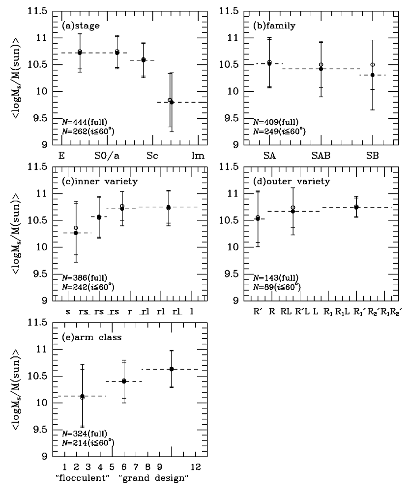
Figure 10: Graphs of the mean log stellar mass of subsets of our AMIGA sample versus morphological structure. Filled circles are for the full (unrestricted by inclination) samples, while open circles are for the subsets restricted to inclination $i$$\leq$60^o. The total numbers of objects in each subset are indicated in each frame. The error bars are 1$\sigma$ standard deviations about the means. The horizontal dashed lines indicate the ranges of morphological features used in the means.

8 Comparative Histogram Analysis

In this section, we use the Kolmogorov-Smirnov test to check for potential morphological biases in Table 3 due to inclination and distance, to look for physical correlations with the environment (Verley et al. 2007b), and to examine the distribution of far-infrared (FIR) excess for bars, rings, and arm classes (Figures 11- 16), In each correlation plot, we show the different morphological $T$-types, families, and inner and outer varieties covered by the histograms.

The p-value of the Kolmogorov-Smirnov test is at the top of each plot and was chosen for our analysis because it effectively quantifies how much two distributions are independent of each other. In the case of a three distribution comparison, we always show the KS test between the two distributions that have the minimum p-value. We consider that two distributions are significantly different when the p-value is lower than 5%. The $p$ values can be sensitive to the number of bins used and to the number of elements involved in the comparison, the result being more accurate when more elements are used.

8.1 Stage, Family, Varieties, and Arm Class

First we look further for bias in the CVRHS classifications by assessing whether the Table 3 classifications are significantly affected by either the source inclination or distance. For example, if bars are more readily recognized in nearby galaxies (potentially due to resolution limitations), then the distributions of barred and non-barred galaxies with distance should be different, with barred galaxies forming a distribution that favours smaller distances. Figure 11 compares the distributions of inner rings (r), outer rings (R), bars (B, AB), and stages with distance (using distances as calculated in Jones et al. 2018); Figure 12 shows similar plots versus galaxy inclination.

The KS test shows a difference between distributions (a p-value of 0.21%) only in the case of the distance distribution versus barred/non-barred galaxies (Figure 11, upper right panel). Due to the relatively small range in redshift across the sample, this difference is not likely due to evolution. In the case of inner (r) and outer (R) rings, a small dependency is found (a p-value of 5.46%). Both galaxies with outer and inner rings in the isolated sample are on average found at slightly larger distances than those without these features.

We repeated the tests above to look for bias due to galaxy inclination (Figure 12), but in all cases we found no apparent dependency, consistent with what we illustrated in Figures 6- 8. However, whether or not a spiral galaxy is identified as either grand design or flocculent is clearly dependent on both distance and inclination. This is illustrated in the top two panels of Figure 16. The sample grand design spirals seem to be more easily identified at lower inclinations and on average are more distant than the sample flocculent spirals. The dependence on inclination may not be unexpected because spiral arm contrast is lower the more inclined the disk galaxy. The dependence on distance could reflect the fact that grand design spirals tend to occur in more luminous systems than do flocculent spirals, and hence can be recognized to greater distances (section 7).

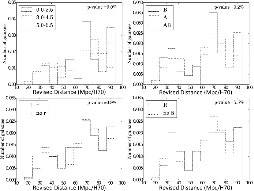
Figure 11: Comparison between the relative frequency of stages, families, inner varieties, and outer varieties in Table 3 as a function of distance $D$ in Mpc. The distances are derived from the observed radial velocities assuming a Hubble constant of $H_{0}$ = 70 km s^-1 Mpc^-1.

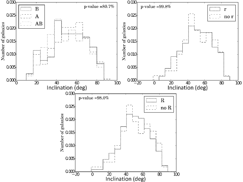
Figure 12: Comparison between the relative frequency of families, inner varieties, and outer varieties in Table 3 as a function of galaxy inclination.

8.2 Morphological features and isolation

Using the same approach as above, we analyzed whether the distributions of two environmental parameters: $\eta_{k}$ and $Q_{Kar,p}$ (Verley et al. 2007b), were altered by restricting to subsamples of specific morphological features. $\eta_{k}$ is the logarithm of the local volume density of neighbouring galaxies, based on the projected separation to the $k$th neighbour and the distance estimate of the galaxy in question (Verley et al. 2007b). Only neighbours that have diameters that are 0.25-4 times that of the target galaxy are considered, as larger (smaller) galaxies are assumed to be foreground (background) objects. However, this does leave open the possibility that some low-mass dwarf companions might be neglected. Typically $k$=5, but in some cases the available optical field is too small to identify 5 neighbours and a lower value of $k$ is used instead. $Q_{Kar,p}$ is a logarithmic and dimensionless measurement of the ratio of a galaxy’s internal gravitational binding force to external tidal forces, which assumes that galaxy diameter is a proxy for total mass (Verley et al. 2007b). For CIG galaxies the mean values of $\eta_{k}$ and $Q_{Kar,p}$ are 1.4 and $-$2.7, and their standard deviations are 0.6 and 0.7, respectively.

Figures 13- 14 show the comparative histograms for stage, family, and inner and outer varieties versus $\eta_{k}$ and $Q_{Kar,p}$; the comparisons for arm class are shown in the middle two panels of Figure 16. We find no dependency on the isolation parameters regarding the detection of inner or outer rings and bars, which could either be a sign of the minimal impact of the environment on the generation of these features, or could be indicating that the scatter in the measurement of the isolation parameters is too large to allow us to distinguish between subtly different environments which do and do not trigger bar/ring formation in isolated galaxies. Another possibility is that isolated galaxies which have bars/rings formed these features in past interactions, although they would probably need to sustain those features for several Gyr, as the AMIGA galaxies have been isolated on that timescale (see section 1).

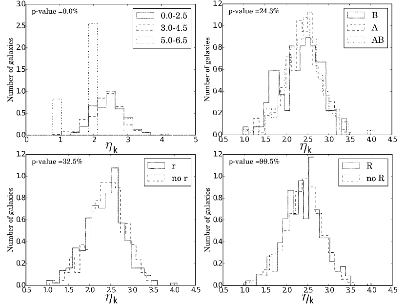
Figure 13: Relative frequencies of stages, families, and inner and outer varieties versus local density parameter $\eta_{k}$.

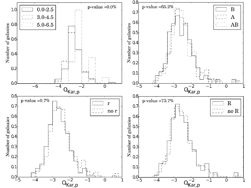
Figure 14: Relative frequencies of stages, families, and inner and outer varieties versus tidal strength parameter $Q_{Kar,p}$.

8.3 Excess of FIR Luminosity

The final parameter we examine is the correlation if any between the morphological features recognized in the Table 3 sample and the FIR excess luminosity. Lisenfeld et al. (2007) derived scaling relations for the AMIGA sample corresponding to $L_{FIR}$ versus $L_{B}$. This fit gives the reference for isolated galaxies, although there is some dispersion within the AMIGA sample itself which is likely due to different degrees of isolation and different formation histories. It is therefore worth checking if there is any correlation between some structural features and a potential excess with respect to the reference $L_{FIR}$, $L_{B}$ relation from that paper (that would correspond to a star formation excess).

Figure 15 shows the distributions for families and inner and outer varieties, while Figure 16 (bottom panel) shows the distribution for arm classes. This FIR deviation is measured according to the best-fit (Lisenfeld et al. 2007) which was estimated by comparing the FIR luminosity and the $B$-band luminosity of the AMIGA sample. Neither bars, rings, nor arm classes for our Table 3 sample show a significant p-value from the KS test.

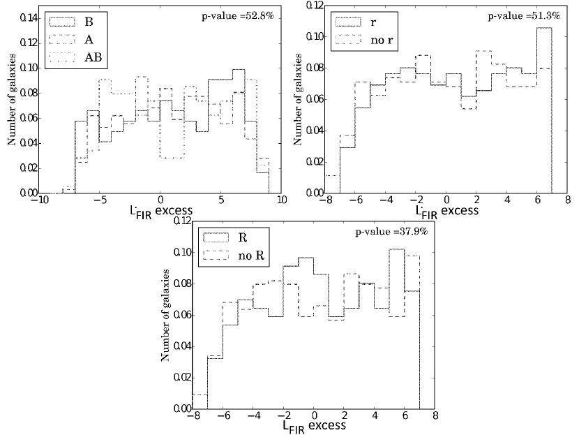
Figure 15: Relative frequencies of stages, families, and inner and outer varieties versus the FIR excess luminosity.

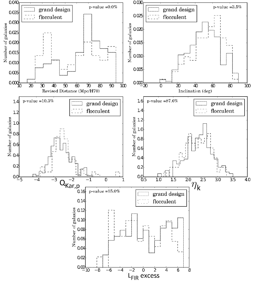
Figure 16: Relative frequencies of arm classes versus distance, inclination, local density parameter $\eta_{k}$, tidal strength parameter $Q_{Kar,p}$, and FIR excess luminosity.

9 Future Studies of Isolated Galaxies

The type of study outlined in this paper depends strongly on the quality of the images used for the classifications. SDSS images have been very useful for this purpose, but new surveys have not only improved on the SDSS, they also cover complementary parts of the sky. For example, the Dark Energy Survey (DES, Abbott et al. 2019) is based on the use of a specially designed wide field camera attached to the Blanco 4-m telescope in Chile and covers 5000 square degrees of mostly southern sky. The Kilo-Degree Survey (KiDS, de Jong et al. 2013) uses the VLT Survey Telescope to cover 1500 square degrees of sky. The Hyper Suprime-Cam Subaru Strategy Program (HSC-SSP, Aihara et al. 2018) and the Large Synoptic Survey Telescope (LSST, Ivezic̀ et al. 2017) are additional future sources of high quality imaging.

Although the goals of these new surveys are mainly cosmology-related (with focus on dark energy and dark matter), the public availability of these imaging databases will facilitate deeper, higher resolution studies of thousands of nearby galaxies. These should allow improved detection in some AMIGA galaxies of faint outer structures, like outer rings or previously unrecognized low surface brightness features, improved resolution of central structures, and also for the improved visibility of very faint and possible small companions in the vicinity of isolated galaxies. There must also be isolated galaxies in parts of the sky that are not covered by the CIG that new surveys will facilitate.

One of the values of the Table 3 classifications is as a training set for automatic classifications of faint galaxies that will be present in the hundreds of thousands to millions on the imaging of these new surveys. Deep machine learning techniques have been shown to be very effective for such a purpose (e.g., Domínguez Sánchez et al. 2018; Dieleman et al. 2015), and Table 3 provides an internally consistent set of classifications that could further facilitate such studies.

10 Summary

We haved carried out a revised classification of 719 AMIGA candidate isolated galaxies from the catalogue of Karachentseva (1973), based on a set of $g$-band digital images from SDSS DR8. The classifications are in the CVRHS system described by Buta et al. (2015). Our main findings are:

1. Consistent with previous studies, spirals are the dominant morphologies, constituting nearly 85% of the sample. Of these, the dominant subtypes are Sb to Sc spirals.

2. Visually strong bars have a low abundance in the AMIGA sample, occurring at the 16% level. Nonbarred galaxies, in contrast, make up $\approx$50% of the sample.

3. (s)-variety spirals (i.e., spirals lacking an inner ring or pseudoring) are the most abundant inner variety subtype, while no outer feature is the most abundant outer variety subtype. In those cases which do have an outer feature, outer pseudorings are the most abundant outer variety subtype. These are not unusual characteristics of a sample dominated by spirals.

4. Grand design spirals are much more abundant in our isolated sample than are flocculent spirals. However, as we have noted, this morphological characteristic could only be reliably judged for 514 of the 597 spiral galaxies recognized in the sample.

5. S$\underline{\rm c}$d and later type galaxies in our sample are less massive than E – Sab galaxies by a factor of nearly 8. This explains why (s)-variety spirals are less massive on average than (r)-variety spirals, SB galaxies are slightly less massive on average than SA galaxies, galaxies with outer rings, lenses, and resonant subclasses are on average more massive than galaxies with ordinary outer pseudorings R^′, and why “grand design" spirals are generally more massive than flocculent spirals.

6. A comparative analysis of the distributions of morphological features of isolated galaxies with distance, inclination, a local density parameter, a tidal strength parameter, and Elmegreen arm class reveals few significant correlations, based on the KS test. There may be a slight distance bias in the recognition of bars in the sample, and there may be both inclination and distance biases in the recognition of arm classes.

We thank an anonymous reviewer for many helpful suggestions which greatly improved this paper. We acknowledge support from grant AYA2015-65973-C3-1-R (MINECO/FEDER, UE). This work has also been supported by the Spanish Science Ministry “Centro de Excelencia Severo Ochoa" Program under grant SEV–2017-0709. M. Jones is supported by a Juan de la Cierva formación fellowship.

References

- (1) Abbott T., et al., 2019, arXiv 1801.03181
- (2) Aihara H., et al., 2011, ApJS, 193, 29
- (3) Aihara H., et al., 2018, PASJ, 70, 84
- (4) Andrae R., Jahnke K., Melchoir P., 2011. 411, 385
- (5) Ann H. B., Seo M., Ha D. K., 2015, ApJS, 217, 27
- (6) Argudo M., Verley S., Bergond G., Sulentic J., Espada D., Santander-Vela J. D., Ruiz J. E., Sabater J., Verdes-Montonegro L., Martínez-Badenes V., 2011, in Highlights of Spanish Physics, Vol. 6, p. 374
- (7) Argudo-Fernández M., Verley S., Bergond G.,Sulentic J.,Sabater J., Fernández-Lorenzo M., Leon S., Espada D., Verdes-Montenegro L., Santander-Vela J. D., Ruiz J. E., Sánchez-Expósito S., 2013, A & A, 560, 9
- (8) Argudo-Hernández M., et al., 2015, A&A, 578, 110
- (9) Baillard A. et al., 2011, A&A, 532, 74
- (10) Baldry I. K., Glazebrook K., Driver S. P., 2008, MNRAS, 388, 945
- (11) Burbidge E. M., Burbidge, G. R., 1960, ApJ, 132, 30
- (12) Burstein D., 1979, ApJ, 234, 829
- (13) Buta R., 1995, ApJS, 96, 39
- (14) Buta R., 2017a, MNRAS, 471, 4027
- (15) Buta R., 2017b, MNRAS, 470, 3819
- (16) Buta R., Combes F., 1996, Galactic Rings, Fund. of Cosmic Physics, 17, 95
- (17) Buta R., Crocker D. A., 1991, AJ, 102, 1715
- (18) Buta R., Crocker D. A., 1993, AJ, 106, 939
- (19) Buta R. J., Corwin H. G., Odewahn S. C., 2007, The de Vaucouleurs Atlas of Galaxies, Cambridge: Cambridge U. Press (dVA)
- (20) Buta R., 2012, Galaxy Morphology, in Secular Evolution of Galaxies, Falcón-Barroso J., Knapen J. H., eds., Cambridge, Cambridge University Press, p. 155
- (21) Buta R., 2013, Galaxy Morphology, in Planets, Stars, & Stellar Systems, Vol. 6, T. D. Oswalt, W. C. Keel, eds., Dordrecht, Springer, p. 1
- (22) Buta R. et al., 2015, ApJS, 217, 32
- (23) Comerón S., Knapen J. H., Beckman J. E., Laurikainen E., Salo H., Martí nez-Valpuesta I., Buta R. J., 2010, MNRAS, 402, 2462
- (24) Comerón S. et al., 2011, ApJ, 741, 28
- (25) Comerón S. et al., 2014, A & A, 562, 121
- (26) Danby, J. M. A., 1965, AJ, 70, 501
- (27) de Jong J. T. A., et al., 2013, The Messenger, 154, 44
- (28) de Vaucouleurs G., 1959, Handbuch der Physik, 53, 275
- (29) de Vaucouleurs G., 1963, ApJS, 8, 31
- (30) de Vaucouleurs G., 1975, ApJS, 29, 193
- (31) de Vaucouleurs G., 1977, in The Evolution of Galaxies and Stellar Populations, B. Tonsley and R. B. Larson, eds., New Haven, Yale University Observatory, p. 43
- (32) de Vaucouleurs G., de Vaucouleurs A., Corwin H. G., Buta R., Paturel G., Fouqué, P., 1991, Third Reference Catalogue of Bright Galaxies, New York, Springer (RC3)
- (33) Dieleman S., Willett K. W., Dambre J., 2015, MNRAS, 450, 1441
- (34) Domínguez Sánchez H., Huertas-Company M., Bernardi M., Tuccillo D., Fischer J., 2018, MNRAS, 476, 3661
- (35) Durbala, A., Buta R., Sulentic J., Verdes-Montenegro L., 2009, MNRAS, 397, 1756
- (36) Durbala, A., Sulentic J., Buta R., Verdes-Montenegro L., 2008, MNRAS, 390, 881
- (37) Elmegreen D., Elmegreen B., 1987, ApJ, 314, 3
- (38) Erwin P., 2004, A&A, 415, 941
- (39) Eskridge P., et al., 2000, AJ, 119, 536
- (40) Espada D., Verdes-Montenegro L., Huchtmeier W., Sulentic J., Verley S., Leon S., Sabater J., 2011, A&A, 532, 117
- (41) Firmani C., Avila-Reese V., 2003, Revista Mexicana de Astronomia y Astrifisica, 17, 107
- (42) Fernández-Lorenzo M., Sulentic J., Verdes-Montenegro L., Ruiz, J., Sabater J., Sánchez S., 2012, A&A, 540, 47
- (43) Fernández-Lorenzo M., Sulentic J., Verdes-Montenegro L., Argudo-Fernández M., 2013, MNRAS, 434, 325
- (44) Fernández-Lorenzo M., et al., 2014, ApJ, 788, 39
- (45) Fukugita M., et al. 2007, AJ, 134, 579
- (46) Gunn J.E., Carr M., Rockosi C. et al., 1998, AJ, 116, 3040
- (47) Ivezić Z., et al., 2019, ApJ, 873, 111
- (48) Jones M. G., Espada D., Verdes-Montenegro L., Huchtmeier W., Lisenfeld U., Leon S., Sulentic J., Sabater J., Jones D. E., Sanchez S., Garrido J., 2018, A & A, 609, 17
- (49) Karachentseva V. E., 1973, Comm. Spec. Ap. Obs., USSR 8, 1
- (50) Kartaltepe J. S., et al. 2016, ApJS, 221, 11
- (51) Kelvin L, et al., 2018, MNRAS, 477, 4116
- (52) Kormendy J., 1979, ApJ, 227, 714
- (53) Kormendy J., 2012, Secular Evolution in Disk Galaxies, in Secular Evolution of Galaxies, Falcón-Barroso J., Knapen J. H., eds., Cambridge, Cambridge University Press, p. 1
- (54) Kormendy J., 2014, in Highlights of Astronomy, T. Montmerle, ed., Cambridge, Cambridge University Press, p. 316
- (55) Kormendy J., Bender R., 1996, ApJ, 464, 119
- (56) Kormendy J., Norman C., 1979, ApJ, 233, 539
- (57) Laurikainen E., Salo H., Athanassoula E., Bosma A., Buta R., Janz J., 2013, MNRAS, 430, 3489
- (58) Leon S., Verdes-Montenegro L., Sabater J., Espada D., Lisenfeld U., Ballu A., Sulentic J., Verley S., Bergond G., García E., 2008, A&A 485, 475
- (59) Lisenfeld U., Verdes-Montenegro L., Sulentic J., Leon S., Espada D., Bergond G., García E., Sabater J., Santander-Vela J., Verley S., 2007, A&A, 462, 507
- (60) Lisenfeld U., Espada D., Verdes-Montenegro L., Kuno N., Leon S., Sabater J., Sato N., Sulentic J., Verley S., Min Y., 2011, A&A, 534, 102
- (61) Martinez-Valpuesta I., Knapen J. H., Buta R., 2007, AJ, 134, 1863
- (62) Naim A., Lahav O., Buta R. J., Corwin H. G., de Vaucouleurs G., Dressler A., Huchra J., van den Bergh S., Raychaudhury S., Sodre L., Storrie-Lombardi M. C., 1995, MNRAS, 274, 1107
- (63) Nair P. B., Abraham R. G., 2010, ApJS, 186, 427
- (64) Paturel G., Fouqué P., Bottinelli L., Gouguenheim L., 1989, A&AS, 80, 299
- (65) Sabater J., Leon S., Verdes-Montenegro L., Lisenfeld U., Sulentic J., Verley S., 2008, A&A, 486, 73
- (66) Sabater J., et al., 2010, ASSP, 14, 349
- (67) Sabater J, Verdes-Montenegro L., Leon S., Best P., Sulentic J., 2012, A&A, 545, 15
- (68) Schweizer F., Whitmore B. C., Rubin V. C., 1983, AJ, 88, 909
- (69) Sheth. K. et al., 2010, PASP, 122, 1397
- (70) Sulentic J., Verdes-Montenegro L., Bergond G., Lisenfeld U., Durbala, A., Espada D., García E., Leon S., Sabater J., Verley S., Casanova V., Sota A. 2006, A&A, 449, 937
- (71) Verdes-Montenegro L., Sulentic J., Lisenfeld U., Leon S., Espada D., García E., Sabater J., Verley S., 2005, A&A, 436, 443
- (72) Verley S., Odewahn S., Verdes-Montenegro L., Leon S., Combes F., Sulentic J., Bergond G., Espada D., García E., Lisenfeld U., Sabater J., 2007a, A&A, 470, 505
- (73) Verley S., Leon S., Verdes-Montenegro L., Combes F., Sabater J., Sulentic J., Bergond G., Espada D., García E., Lisenfeld U., Odewahn S., 2007b, A&A, 472, 121
- (74) Verley S., Combes F., Verdes-Montenegro L., Bergond G., Leon S., 2007c, A&A, 474, 43
- (75) York D. G., Adelman J., Anderson J. E. et al., 2000, AJ, 120, 1579