Reduced-Order Quasilinear Model of Ocean Boundary-Layer Turbulence

Abstract

The combined effectiveness of model reduction and the quasilinear approximation for the reproduction of the low-order statistics of oceanic surface boundary-layer turbulence is investigated. Idealized horizontally homogeneous problems of surface-forced thermal convection and Langmuir turbulence are studied in detail. Model reduction is achieved with a Galerkin projection of the governing equations onto an subset of modes determined by proper orthogonal decomposition. For less than 0.2% of the modes retained, the reduced quasilinear model is able to reproduce vertical profiles of horizontal mean fields as well as certain energetically important second-order turbulent transport statistics and energies to within 30% error. For intermediate sizes of the basis truncation some statistics approach those found in the fully nonlinear simulations. Thus basis reduction can actually improve upon the accuracy of quasilinear dynamics. A test model with a small total number of modes demonstrates the non-monotonic convergence toward the correct statistics as the size of the basis is increased.

1 Introduction

Reliable weather and climate modeling requires the accurate simulation of two turbulent components of the Earth system that have thus far only seen incremental improvements: the oceanic and atmospheric boundary layers (BLs). Given that long duration turbulence-resolving simulation is centuries beyond the reach of present-day computers (Fox-Kemper et al. 2014; Stocker et al. 2013; Hamlington et al. 2014), large-scale numerical simulations of the Earth’s oceans and atmospheres employ the hydrostatic primitive equations, in which vertical accelerations of fluid parcels are presumed negligible, enabling significant computational savings. Unfortunately, predictions of vertical transport and mixing are generally unreliable as these depend crucially on smaller-scale, non-hydrostatic 3D processes – particularly turbulence within the planetary BL (McWilliams and Sullivan 2000) – that are neglected or phenomenologically parameterized. Errors in the simulation of low clouds, for example, are believed to be the single most important source of uncertainty in climate models and have stymied effort at improvement (Bony et al. 2015; Stephens 2005). Similarly, wind- and surface-wave-driven Langmuir turbulence in the ocean surface BL should be incorporated into climate models for improved accuracy and robustness (Belcher et al. 2012), yet a recent ocean BL simulation with horizontal grid spacing near 4 meters required millions of supercomputer hours for only weeks of simulated time to capture a region only 20km $\times$ 20km (Hamlington et al. 2014).

Given that convective turbulence mediates vertical exchanges both within and between the atmospheric and oceanic BLs, it is perhaps not surprising that general circulation models are very sensitive to the chosen parameterizations of vertical transport (Large et al. 1997; Doney et al. 2004; Fox-Kemper and Ferrari 2008; Li et al. 2019). The present unsatisfactory state-of-affairs is summarized in a review of numerical weather prediction, which asserts “the uncertainties inherent to physical parameterization, either from incomplete process understanding or the dilemma of representing the impact of unresolved processes on the resolved scales, may require a fundamentally different approach. Elements of parameterizations or entire schemes are likely to require components that appear statistical to the large scales. Examples are stochastic sampling of parameter probability distribution functions, stochastically driven sub-cell models, or super-parameterizations through embedding entire convection-resolving simulations at sub-grid scale $\ldots$ How radical this approach needs to be is currently not clear” (Bauer et al. 2015).

The systematic development of Direct Statistical Simulation (DSS) approaches to the oceanic boundary layer is our central objective here. As a first step in that direction we employ the quasi-linear (QL) approximation (Malkus 1954; Vedenov et al. 1961; Spiegel 1962; Herring 1963; Marston et al. 2019) for which a non-local second-order closure (described below) is exact. Chaalal et al. (2016) investigated the QL approximation in a related model of the dry convective atmospheric boundary layer, demonstrating that QL can capture BL deepening and, with less accuracy, the turbulent transport of kinetic energy. Two ocean-surface boundary layer models will be used for case studies: Surface-forced thermal convection and Langmuir turbulence (Leibovich 1983; Thorpe 2004). Both problems are statistically homogeneous in the horizontal, while Langmuir and, if subjected to wind shear, convective turbulence additionally are anisotropic in the horizontal (Van Roekel et al. 2012). We emphasize that, owing to horizontal isotropy, this configuration constitutes a particularly challenging application for DSS, yet one of fundamental geoscientific importance.

Eschewing the traditional route of accumulating statistics from numerical simulation time series, DSS is a set of approaches for directly obtaining the statistics of dynamical systems rather than by their accumulation from numerical simulation (Allawala and Marston 2016). One form of DSS focuses on the equations of motion (EOM) for the equal-time cumulants, which are truncated at low order. Consider modeling the evolution of a state vector ${\bf q}(\vec{{r}},t)$ specified by a system of master partial differential equations (PDEs). For simplicity, further consider the case where the nonlinearities are quadratic so that the system can be written as

$${\bf q}_{t}={\cal L}[{\bf q}]+{\cal Q}[{\bf q},{\bf q}],$$ (1)

where ${\cal L}$ is a linear vector differential operator and ${\cal Q}$ is the operator that includes the nonlinear (quadratic) interactions such as those arising in the material derivative. Specializing to models that are translationally invariant in one direction, henceforth denoted the zonal (or streamwise) direction, a standard Reynolds decomposition of the state vector into its zonal mean and fluctuation (denoted with an overbar and prime, respectively) is made by setting ${\bf q}=\overline{{\bf q}}+{{\bf q}^{\prime}}$. The average here is chosen to satisfy the Reynolds rules of averaging so that $\overline{\overline{\bf q}}=\overline{\bf q}\ \ {\rm and}\ \ \overline{{\bf q}^{\prime}}=0$. Averaging Eqn. (1), using the linearity of ${\cal L}$ and assuming the averaging operator commutes with ${\cal L}$, yields

$$\overline{{\bf q}}_{t} = \overline{{\cal L}[{{\bf q}}]}+\overline{{\cal Q}[{\bf q},~{}{\bf q}]}\;=\;{\cal L}[\overline{{\bf q}}]+\overline{{\cal Q}[{\bf q},~{}{\bf q}]}.$$ (2)

Of course, the difficulty now is to describe the average of the nonlinear term in the equation for the mean (the first cumulant). At this point local closure schemes are often adopted (Krause and Raedler 1980; Rüdiger 1989). For example, in large-eddy simulations (LES) of turbulent flows, the average of this nonlinear term is generally parameterized using Fickian diffusive schemes in which fluctuation correlations are taken to be proportional to the (local) gradient of mean variables (Canuto and Minotti 2001). Not only are such closures inaccurate and not mathematically justifiable for inhomogeneous and anisotropic flows, but in LES the ad hoc proportionality coefficients must be trained for particular flow regimes. Standard LES schemes are particularly ineffective near walls (when additional ad hoc, e.g. Van Driest, wall models are required) and for strongly anisotropic flows, including strongly stratified turbulence.

A more sophisticated approach is to derive an equation for the evolution of the mean of the non-local fluctuation–fluctuation (or eddy–eddy) interactions (Bartello and Holloway 1991; Maltrud and Vallis 1991). Unwarranted assumptions about homogeneity or isotropy are avoided, and non-local correlations of the form $\overline{{\bf q}^{\prime}(\vec{r}_{1}){\bf q}^{\prime}(\vec{r}_{2})}$ are tracked, where $\vec{r}_{1}$ and $\vec{r}_{2}$ are two position vectors within the domain of interest (Marston et al. 2008). The equation governing the evolution of this quantity (the second cumulant) is obtained by multiplying the EOM for the system (defined at the point $\vec{r}_{1}$) by ${\bf q}(\vec{r}_{2})$, averaging and symmetrizing. In addition to introducing non-local quadratic terms from the $\overline{{\bf q}\,{\cal L}[{\bf q]}}$ terms, this procedure requires the evaluation of non-local cubic terms (the third cumulant) that arise from the $\overline{{\bf q}\,{\cal Q}[{\bf q},{\bf q}]}$ terms in Eqn. (1). The simplest and most computationally efficient approach is to truncate the hierarchy at second order by dropping the contribution of the third cumulant, $\overline{{\bf q}^{\prime}(\vec{r}_{1}){\bf q}^{\prime}(\vec{r}_{2}){\bf q}^{\prime}(\vec{r}_{3})}$, to the EOM for the second. Termed CE2 in Marston et al. (2008); Marston (2010) and S3T in Farrell and Ioannou (2007), this truncation of the cumulant expansion (CE) at second order is both a conservative and realizable approximation (Salmon 1998). Furthermore, CE2 is quasilinear in the sense that it includes interactions of mean quantities with eddies to give eddies and interactions of eddies with eddies to give mean flows, but neglects eddy-eddy scattering. Equivalently, it is readily shown that by invoking a QL approximation of the instantaneous dynamics, the same closed equations for the first two cumulants are obtained (Farrell and Ioannou 2007; Marston et al. 2008; Srinivasan and Young 2012b).

While ineffective for homogeneous isotropic turbulence, the quasilinear approximation has been shown to qualitatively (and in some cases, quantitatively) reproduce mean flows and two-point correlation functions for model problems describing a wide range of anisotropic and heterogeneous flows. Specifically, QL has been successfully utilized to describe the driving of mean flows in plasmas and on giant planets (Tobias et al. 2011), the sustenance of wall-bounded shear-flow turbulence (Thomas et al. 2015), the growth of a dry atmospheric convective boundary layer (Chaalal et al. 2016), and even the development of the magnetorotational instability in accretion discs (Squire and Bhattacharjee 2015). The QL approximation is thought to be suitable to planetary flows because of the relative importance of interactions between small-scale eddies and mean-field flow features (O’Gorman and Schneider 2007). Recently, the suitability of this approximation for planetary boundary-layer applications has been supported by demonstrations of the emergence of zonal jets on a randomly or stochastically forced $\beta$-plane (Srinivasan and Young 2012a; Tobias and Marston 2013) and the statistics of thermal instabilities in the atmospheric boundary layer (Chaalal et al. 2016) under QL dynamics or statistically equivalent frameworks. Furthermore, the QL approximation has substantial capacity for improvement through variations on the exact statistical closure of the cumulant expansion of QL systems (such as CE2.5 and CE3 (Marston et al. 2019)) and extensions such as the generalized quasilinear approximation (GQL) (Marston et al. 2016).

The quasilinear approximation has a number of mathematically attractive attributes.

• QL can be shown to be exact in appropriate asymptotic limits (e.g. for strong mean flows or for an extreme separation of time scales) (Bouchet et al. 2013) and, in regimes away from the strict asymptotic limit, errors can be controlled and reduced by methodically retaining higher-order cumulants.

• QL retains the quadratic conservation properties of the underlying master PDEs and is realizable, implying a non-negative probability distribution.

• The low-order statistics found with QL vary more smoothly than do instantaneous flow-field realizations, suggesting the possibility of dimension reduction in numerical simulations (Allawala et al. 2017).

• The attractor for the low-order statistical dynamical evolution may be much simpler (e.g. an equilibrium point or limit cycle) than that characterizing the instantaneous (generally turbulent) dynamics, and the temporal evolution of the low-order statistics is comparably stiff, implying that these simple attractors should be mored readily accessible.

For all its virtues, the quasilinear approximation nevertheless suffers from two primary deficiencies.

• Insufficient accuracy: QL is deficient as the system is driven harder, reducing time-scale separation between the strict mean flow and the faster dynamics. This limitation was demonstrated in Tobias and Marston (2013), which compared the statistics derived from DNS for the problem of driving $\beta$-plane jets. QL reproduced both the number and strength of jets for large time-scale separation but failed as the system was driven further away from equilibrium. In practice, attempts to correct this deficiency by retaining higher-order cumulants are fraught with difficulty (e.g. the non-realizability of CE3). More generally, higher-order cumulant expansions rapidly become analytically and computationally unwieldy.

• Computational expense: Although infrequently discussed in the research literature, naive implementations of QL/CE2 schemes actually can be as or even more expensive than full DNS because the second cumulant may have higher dimensionality than the underlying fields (depending upon the symmetries of the problem and the choice of averaging operation). Extending the level of truncation by one order requires the calculation of correlations with an extra point in space, increasing the degrees of freedom of the system by $D$ where $D$ is the dimensionality of the system. Consequently, in practice, attempts to increase the accuracy of CE2 by retaining higher-order cumulants are computationally prohibitive.

We show below that both of these deficiencies can be addressed simultaneously by dimensional reduction of the boundary-layer models using Proper Orthogonal Decomposition (POD). POD, a method closely related to Empirical Orthogonal Functions (EOF) and Principal Component Analysis (PCA), is a common means to generate a reduced basis for applications in computational fluid dynamics in which the representation of a flow is decomposed into a set of modes based on the amount of variation in the flow that they describe in terms of energy (Holmes et al. 2012). Often, POD reduced models will retain only the most energetic of these modes. When the QL approximation is defined with respect to a spatial average over statistically homogeneous dimensions, it eliminates the direct flow of energy between scales in those dimensions; as a result, energy tends to populate fewer modes than with fully nonlinear (NL) dynamics. The use of energy optimization is a particularly suitable pairing for the QL approximation then because fewer modes must be retained to capture a similar portion of the variation in the flow than with NL dynamics.

Another motivation for combining POD with QL when defined with a spatial average over a homogeneous dimension is that the statistics are invariant under a phase shift of individual Fourier modes in that dimension, implying that the phases of different Fourier modes are uncorrelated and localized structures cannot be captured in the flow solutions (see section 2 of this paper, also Skitka (2019)). Because POD modes must be horizontal Fourier modes due to translational symmetry in the ensemble of flow realizations (see appendix A), POD washes away localized coherent structures that could otherwise be represented with very few coherent modes. (Sirovich (1989) notes a $\mathcal{O}\left(10^{3}\right)$ - $\mathcal{O}\left(10^{4}\right)$ reduction in the POD dimensionality of Rayleigh-Bénard convection when rigid walls break the symmetry of an otherwise periodic case.) The resulting bases have no encoded phase correlations, making the application of POD to homogeneous dimensions suited to the application of quasilinear approximation to spatial averages.

Recently, Allawala et al. (2017) have demonstrated that accurate statistics for 2D rotating geostrophic flow on a sphere (a zonally-homogeneous, anisotropic, stationary problem) can be retained at massive dimensional reduction with a POD reduced model of CE2, an exact statistical closure of QL. Additionally, NL POD reduced models often suffer from a buildup of energy because energy pathways to the myriad small scales must be omitted, similar to an LES-simulation near the cutoff length (Wang et al. 2012). In QL POD reduced models, small scales only exchange energy with with the mean flow along statistically homogeneous dimensions, thus there can only be an indirect buildup of energy at cutoff scales through the modification of the mean flow rather than a direct local buildup between scales. In light of this, it might be expected that QL POD reduced models would have better stability properties than NL POD reduced models.

The particular problems used as test cases here, surface-driven convection into stratification and Langmuir turbulence, are classic problems in planetary boundary layers (Foken 2006; Large et al. 1994; McWilliams et al. 1997). They are of immediate importance to global climate modeling in both the ocean (Belcher et al. 2012) and atmosphere (Kang et al. 2009). From the oceanographic perspective, other problems such as submesoscale mixed layer eddy restratification (Fox-Kemper and Ferrari 2008) or mixing by symmetric instability (Bachman et al. 2017) are seemingly similar: inhabiting the boundary layer and affecting the balance between mixing and restratification. However, from the generalized symmetry perspective submesoscale turbulence differs fundamentally, as it only exists in the presence of horizontal density gradients, thus these problems have horizontal homogeneity in only one direction. The general approach here applies to boundary layer turbulence that oceanographers call “vertical mixing” and atmospheric modelers call “pencil models”, both of which are horizontally homogeneous in both directions and heterogeneous in the vertical.

In one important way, the approach taken here resembles that of Mellor and Yamada (1974): it relies on a structured sequence of approximations of increasingly higher moments. However, Mellor-Yamada SGS models (and relatives for Langmuir turbulence, e.g., Harcourt 2013) tend to emphasize moments that are co-located in vertical position. Doing so reduces the dimensionality of the problem, but it prevents non-local effects from playing a leading role in the scheme dynamics. Non-local effects and relative motions are fundamental to the statistics of turbulence, as frequently demonstrated using structure functions and two-point correlations (Kolmogorov 1941; Batchelor 1952). However, allowing a SGS scheme to depend on non-local statistics means that the dimensionality of the analysis increases. For example, for a horizontally-homogeneous, stationary problem, one-point statistics will depend only on vertical position, while two-point, equal-time statistics depend on two independent vertical positions and their horizontal separation vector. Thus, a non-local approach is potentially more powerful, but not obviously efficient.

This article first describes the theory underpinning the proposed model framework in section 2, including that of POD Reduced Modeling, the QL approximation, and how basic assumptions appropriate for ocean surface boundary layers, specifically horizontal homogeneity, can be used to make simplifications. Section 3 covers the numerical implementation of the this framework, including an introduction to a custom-built reduced-model solver. Section 4 defines the two examples of ocean surface boundary-layer turbulence that are used to test this technique. The results of the QL reduced-model runs are presented in section 5 while discussion of the implications of these results as well as promising areas of future research are reserved for section 6.

2 Theoretical Framework

In POD, the flow is decomposed using the eigenvectors of the uncentered, equal-time covariance matrix, $\mathsf{R}$. Let the flow variables be written $\mathbf{q}=\left(q_{1}\left(t\right)\;,\;\;\;\dots\;\;\;q_{N}\left(t\right)\right)^{\top}$, where the index runs over discretized spatial coordinates as well as fields (e.g. velocity, temperature), $t$ is the undiscretized time, and $N$ is the total number of flow variables. Returning to the Reynolds decomposition introduced in section 1), $\mathbf{q}=\overline{\mathbf{q}}+\mathbf{q}^{\prime}$ where $\overline{\mathbf{q}}$ indicates the mean fields under a generic averaging procedure and $\mathbf{q}^{\prime}$ indicates the fluctuating component of the fields, then

$$\mathsf{R}_{ij}=\overline{q_{i}q_{j}}\;\textrm{;}\;\mathsf{R}=\frac{1}{M}\sum_{1\leq s\leq M}\bm{q_{s}}\bm{q_{s}}^{\top}$$ (3)

where the indices $i$ and $j$ indicate both field and position. $s$ indicates the field snapshot, of which there are $M$; these are sampled from different times and/or ensemble members. The eigendecomposition of $\mathsf{R}$ is:

$$\mathsf{R}\bm{\Phi}^{\alpha}=\lambda^{\alpha}\bm{\Phi}^{\alpha}$$ (4)

A truncated basis retains the most energetic modes, $\bm{\Phi}^{\alpha}$, as indicated by the associated eigenvalues, $\lambda^{\alpha}$. The naked $\phi^{\alpha}$ will be reserved for the amplitudes of a flow field in the POD representation, whereas $\bm{\Phi}^{\alpha}$ can be thought of as the unit vector of a basis for flow states,

$$q_{i}=\sum_{1\leq\alpha\leq N}\phi^{\alpha}\bm{\Phi}_{i}^{\alpha},$$

for some coefficients $\phi^{\alpha}$, where $N\leq M$ is the number of independent modes spanned by the $M$ snapshots.

Because the cases of SGS turbulence are intended to be small in horizontal extent, ignoring horizontal inhomogeneities in the flow forcing is a reasonable approximation that will be important for allowing the POD reduced model to be performed efficiently on a large, three-dimensional problem. For horizontally homogeneous cases, which will be used exclusively in this work, covariances may be constrained to depend on only the separation vector between two flow variables, and it follows that POD modes are constrained to be horizontal Fourier modes (see appendix A for a derivation of this.) This allows for the POD eigendecomposition (equation 4) to be performed individually for each horizontal Fourier mode. To apply this to discrete flow fields as they are represented in a solver, the fields are written in terms of their horizontal Fourier wavenumber vector index, $\mathbf{m}_{i}=\left\{m_{i},l_{i}\right\}$ and their vertical position and field index, $z_{i}$. Here $m_{i}$ and $l_{i}$ are the horizontal, $x$ and $y$ directed wavenumber indices. Individual POD modes from equation 4 now need only be labeled with their horizontal wavenumber and an additional index, $k_{\alpha}$, corresponding to the degrees of freedom associated with the vertical direction and the different fields: $\bm{\Phi}^{\alpha}=\bm{\Phi}_{\mathbf{m}_{\alpha},k_{\alpha}}$ and may be defined by a discrete vertical profile:

$$\bm{\Phi^{\alpha}}=\left(\Phi_{\mathbf{m}_{\alpha},k_{\alpha},z_{1}}\;,\;\;\;\dots\;\;\;,\;\;\;\Phi_{\mathbf{m}_{\alpha},k_{\alpha},z_{N_{z}}}\right)^{\top}$$ (5)

Let the evolution of field variables, $q$, be written in terms of generic constant, $\mathsf{C}$, linear, $\mathsf{L}$, and quadratic, $\mathsf{Q}$, operators in the horizontal Fourier basis and vertical position basis.

$$\partial_{t}q_{\mathbf{m}_{i},z_{i}}\left(t\right) =\mathsf{Q}_{\mathbf{m}_{i},z_{i};\mathbf{m}_{j},z_{j};\mathbf{m}_{l},z_{l}}q_{\mathbf{m}_{j},z_{j}}\left(t\right)q_{\mathbf{m}_{l},z_{l}}\left(t\right)$$

$$\quad+\mathsf{L}_{\mathbf{m}_{i},z_{i};\mathbf{m}_{j},z_{j}}q_{\mathbf{m}_{j},z_{j}}\left(t\right)+\mathsf{C}_{\mathbf{m}_{i},z_{i}}$$ (6)

where $t$ is the undiscretized time and repeated indices imply a sum. Hereafter, $t$ will be dropped and all field variables will be assumed to have an implicit time coordinate and for the remainder of this section, $z$ will run over vertical positions and fields. Note that many elements in the implied summations will be exactly zero, allowing for the equations to be constrained in terms of the allowable horizontal wavenumbers in subsequent equations.

As an example of the generic operator decomposition in equation 6, consider a basic temperature advection equation, $\partial_{t}T+\left(\mathbf{u}\cdot\bm{\nabla}\right)T=F_{T}+\kappa\nabla^{2}T$, where $T$ is the temperature, $\mathbf{u}$ is the 3-dimensional velocity field, $F_{T}$ accounts for external forcing, and $\kappa$ is the thermal diffusivity of a fluid. Here, $\mathsf{Q}$ would be a tensor strictly defined by the discretized advective term, $\mathsf{L}$ would be defined by the diffusive term, and $\mathsf{C}$ would be defined by the external forcing. In fluids, the continuum equations that govern fully resolved flows do not have terms that are higher than second-order in the field variables, so this generalized notation is an accurate starting point for developing a SGS model.

The quasilinear approximation neglects the scattering of eddy fields, $q^{\prime}=q_{\mathbf{m}\neq\mathbf{0}}$, into other eddy fields, thereby eliminating the scale-by-scale transfer of energy between horizontal length scales; rather, all energy transfer to or from a given length-scale of turbulence must be with the mean field, $\overline{q}=q_{\mathbf{m}=\mathbf{0}}$. This omits the scale-by-scale cascade of turbulent energy and enstrophy. Assuming the evolution coefficients $\mathsf{Q}$, $\mathsf{L}$, and $\mathsf{C}$ are also horizontally homogeneous, the quadratic and linear operators are constrained to just the interacting “triads” of the quadratic term interactions within vertical water columns:

$$\mathsf{Q}_{\mathbf{m}_{i},z_{i};\mathbf{m}_{j},z_{j};\mathbf{m}_{l},z_{l}} =\tilde{\delta}_{\mathbf{m}_{i}-\mathbf{m}_{j}-\mathbf{m}_{l}}\mathsf{Q}_{\mathbf{m}_{i},z_{i};\mathbf{m}_{j},z_{j};\mathbf{m}_{l},z_{l}}$$ (7)

$$\mathsf{L}_{\mathbf{m}_{i},z_{i};\mathbf{m}_{j},z_{j}} =\tilde{\delta}_{\mathbf{m}_{i}-\mathbf{m}_{j}}\mathsf{L}_{\mathbf{m}_{i},z_{i};\mathbf{m}_{j},z_{j}}$$ (8)

where $\tilde{\delta}_{\mathbf{m}}$ is a modified Kronecker delta:

$$\tilde{\delta}_{\mathbf{m}}=\delta_{\textrm{MOD}\left[\mathbf{m}_{i}\right],\mathbf{0}}=\delta_{m\;mod\;N_{x},0}\delta_{l\;mod\;N_{y},0}$$ (9)

Then the subset of the coefficients not constrained to be zero within this context may be written

$$\mathsf{Q}_{\mathbf{m}_{i},\mathbf{m}_{j},z_{i},z_{j},z_{l}} =\mathsf{Q}_{\mathbf{m}_{i},z_{i};\mathbf{m}_{j},z_{j};\mathbf{m}_{i}-\mathbf{m}_{j},z_{l}}$$ (10)

$$\mathsf{L}_{\mathbf{m}_{i},z_{i},z_{j}} =\mathsf{L}_{\mathbf{m}_{i},z_{i};\mathbf{m}_{i},z_{j}}$$ (11)

Note that the wavenumber indices of the coefficients $\mathsf{Q}_{\mathbf{m}_{i},\mathbf{m}_{j},\dots}$ and $\mathsf{L}_{\mathbf{m}_{i},\dots}$ implicitly have a $\textrm{MOD}\left[\mathbf{m}_{i}\right]$ acting on them. Then, using the convention that sums over a basis index are implied when the associated vertical index is repeated (e.g. sum over $j$ for repeated $z_{j}$) and that all mean-field Fourier modes (including differences such as $\mathbf{m}_{i}-\mathbf{m}_{j}$) are explicitly written as $\mathbf{0}$, the full-basis quasilinear equations are:

$$\partial_{t}q\left(\mathbf{0},z_{i}\right)=$$

$$\quad\mathsf{Q}_{\mathbf{0},\mathbf{m}_{j},z_{i},z_{j},z_{l}}q\left(\mathbf{m}_{j},z_{j}\right)q\left(-\mathbf{m}_{j},z_{l}\right)$$

$$\quad+\mathsf{Q}_{\mathbf{0},\mathbf{0},z_{i},z_{j},z_{l}}q\left(\mathbf{0},z_{j}\right)q\left(\mathbf{0},z_{l}\right)$$

$$\quad+\mathsf{L}_{\mathbf{0},z_{i},z_{j}}q\left(\mathbf{0},z_{j}\right)+\mathsf{C}_{\mathbf{0},z_{i}}$$ (12)

$$\partial_{t}q\left(\mathbf{m}_{i},z_{i}\right)=$$

$$\quad\hbox to0.0pt{\raisebox{2.25002pt}{{\color[rgb]{.5,.5,.5}\rule{122.30429pt}{2.0pt}}}\hss}\mathsf{Q}_{\mathbf{m}_{i},\mathbf{m}_{j},z_{i},z_{j},z_{l}}q\left(\mathbf{m}_{j},z_{j}\right)q\left(\mathbf{m}_{i}-\mathbf{m}_{j},z_{l}\right)$$

$$\quad+\mathsf{Q}_{\mathbf{m}_{i},\mathbf{m}_{i},z_{i},z_{j},z_{l}}q\left(\mathbf{m}_{i},z_{j}\right)q\left(\mathbf{0},z_{l}\right)$$

$$\quad+\mathsf{Q}_{\mathbf{m}_{i},\mathbf{0},z_{i},z_{j},z_{l}}q\left(\mathbf{0},z_{j}\right)q\left(\mathbf{m}_{i},z_{l}\right)$$

$$\quad+\mathsf{L}_{\mathbf{m}_{i},z_{i},z_{j}}q\left(\mathbf{m}_{i},z_{j}\right)+\mathsf{C}_{\mathbf{m}_{i},z_{i}}$$ (13)

where the omitted nonlinear term is indicated by the strikethrough. This expression of the quasilinear approximation in terms of Fourier modes more readily reveals a key feature and, depending on the circumstance, shortcoming of using spatial averages to define QL. Assume that $\mathsf{C}_{\mathbf{m}_{i},z_{i}}=0$, as is true for all cases studied in this paper. Noting that all terms of the HQL eddy-field evolution (equation 13) are linear in $q^{\prime}\left(\mathbf{m}_{n}\right)$ and all terms in the HQL mean-field evolution (equation 12) are constant or bilinear in $q^{\prime}\left(\mathbf{m}_{n}\right)$, the HQL equations are seen to be invariant under an independent phase shift (Pausch et al. 2019) for each set of all eddy modes of a specific horizontal wavenumber, $\mathbf{m}_{n}$. It follows that the relative phases of horizontal Fourier modes in the eddy field must only depend on the initial conditions; if these initial conditions are randomly sampled, the phases of different Fourier modes, being blind to one another, will be uncorrelated, and it is unlikely that localized structures will appear; rather, flow features in the horizontal direction (or, by extension, any homogeneous dimension of averaging used for QL) will be strictly wavelike and nonlocal, something that will manifest visually distinctly in HQL flow fields observed in the results (section 5).

A reduced model may be derived by projecting the dynamical equations of motion (equation 6) onto a truncated reduced basis. Let the POD field amplitude be written:

$$\phi_{\alpha}=\phi_{\mathbf{m}_{\alpha},k_{\alpha}}=\sum_{j}q_{\mathbf{m}_{\alpha},z_{j}}\Phi_{\mathbf{m}_{\alpha},k_{\alpha},z_{j}}^{*}$$ (14)

then the Galerkin projection of the equations of motion onto this basis is

$$\partial_{t}\phi_{\mathbf{m}_{\alpha},k_{\alpha}} =$$

$$\bm{\Phi}_{\mathbf{m}_{\alpha},k_{\alpha},z_{i}}^{*}\mathsf{Q}_{\mathbf{m}_{\alpha},\mathbf{m}_{\sigma},z_{i},z_{j},z_{l}}\bm{\Phi}_{\mathbf{m}_{\sigma},k_{\sigma},z_{j}}$$

$$\qquad\qquad\qquad\bm{\Phi}_{\mathbf{m}_{\alpha}-\mathbf{m}_{\sigma},k_{\beta},z_{l}}\phi_{\mathbf{m}_{\sigma},k_{\sigma}}\phi_{\mathbf{m}_{\alpha}-\mathbf{m}_{\sigma},k_{\beta}}$$

$$+\bm{\Phi}_{\mathbf{m}_{\alpha},k_{\alpha},z_{i}}^{*}\mathsf{L}_{\mathbf{m}_{\alpha},z_{i},z_{j}}\bm{\Phi}_{\mathbf{m}_{\alpha},k_{\sigma},z_{j}}\phi_{\mathbf{m}_{\alpha},k_{\sigma}}$$

$$+\bm{\Phi}_{\mathbf{m}_{\alpha},k_{\alpha},z_{i}}^{*}\mathsf{C}_{\mathbf{m}_{\alpha},z_{i}}$$ (15)

where summations are now implied when either vertical index is repeated within a term (e.g., sum over $j$ for repeated $k_{j}$ or $z_{j}$). By defining the truncated evolution coefficients as

$$\tilde{\mathsf{Q}}_{\mathbf{m}_{\alpha},\mathbf{m}_{\sigma},k_{\alpha},k_{\sigma},k_{\beta}}=$$

$$\qquad\bm{\Phi}_{\mathbf{m}_{\alpha},k_{\alpha},z_{i}}^{*}\mathsf{Q}_{\mathbf{m}_{\alpha},\mathbf{m}_{\sigma},z_{i},z_{j},z_{l}}\bm{\Phi}_{\mathbf{m}_{\sigma},k_{\sigma},z_{j}}\bm{\Phi}_{\mathbf{m}_{\alpha}-\mathbf{m}_{\sigma},k_{\beta},z_{l}}$$ (16)

$$\tilde{\mathsf{L}}_{\mathbf{m}_{\alpha},k_{\alpha},k_{\sigma}}=\bm{\Phi}_{\mathbf{m}_{\alpha},k_{\alpha},z_{i}}^{*}\mathsf{L}_{\mathbf{m}_{\alpha},z_{i},z_{j}}\bm{\Phi}_{\mathbf{m}_{\alpha},k_{\sigma},z_{j}}$$ (17)

$$\tilde{\mathsf{C}}_{\mathbf{m}_{\alpha},k_{\alpha}}=\bm{\Phi}_{\mathbf{m}_{\alpha},k_{\alpha},z_{i}}^{*}\mathsf{C}_{\mathbf{m}_{\alpha},z_{i}}$$ (18)

the truncated evolution equations may be succinctly expressed as

$$\partial_{t}\phi_{\mathbf{0},k_{\alpha}}=$$

$$\quad\tilde{\mathsf{Q}}_{\mathbf{0},\mathbf{m}_{\beta},k_{\alpha},k_{\beta},k_{\gamma}}\phi_{\mathbf{m}_{\beta},k_{\beta}}\phi_{-\mathbf{m}_{\beta},k_{\gamma}}$$

$$\quad+\tilde{\mathsf{Q}}_{\mathbf{0},\mathbf{0},k_{\alpha},k_{\beta},k_{\gamma}}\phi_{\mathbf{0},k_{\beta}}\phi_{\mathbf{0},k_{\gamma}}$$

$$\quad+\tilde{\mathsf{L}}_{\mathbf{0},k_{\alpha},k_{\beta}}\phi_{\mathbf{0},k_{\beta}}+\tilde{\mathsf{C}}_{\mathbf{0},k_{\alpha}}$$ (19)

$$\partial_{t}\phi_{\mathbf{m}_{\alpha},k_{\alpha}}=$$

$$\quad\hbox to0.0pt{\raisebox{2.16669pt}{{\color[rgb]{.5,.5,.5}\rule{85.96854pt}{2.0pt}}}\hss}\tilde{\mathsf{Q}}_{\mathbf{m}_{\alpha},\mathbf{m}_{\beta},k_{\alpha},k_{\beta},k_{\gamma}}\phi_{\mathbf{m}_{\beta},k_{\beta}}\phi_{\mathbf{m}_{\alpha}-\mathbf{m}_{\beta},k_{\gamma}}$$

$$\quad+\tilde{\mathsf{Q}}_{\mathbf{m}_{\alpha},\mathbf{m}_{\alpha},k_{\alpha},k_{\beta},k_{\gamma}}\phi_{\mathbf{m}_{\alpha},k_{\beta}}\phi_{\mathbf{0},k_{\gamma}}$$

$$\quad+\tilde{\mathsf{Q}}_{\mathbf{m}_{\alpha},\mathbf{0},k_{\alpha},k_{\beta},k_{\gamma}}\phi_{\mathbf{0},k_{\beta}}\phi_{\mathbf{m}_{\alpha},k_{\gamma}}$$

$$\quad+\tilde{\mathsf{L}}_{\mathbf{m}_{\alpha},k_{\alpha},k_{\beta}}\phi_{\mathbf{m}_{\alpha},k_{\beta}}+\tilde{\mathsf{C}}_{\mathbf{m}_{\alpha},k_{\alpha}}$$ (20)

The horizontal strikethrough indicates the terms omitted in the reduced quasilinear approximation.

3 Numerical Implementation

In order to compute the reduced basis for a specific, developing flow case, an ensemble of 24 members was run using full-basis quasilinear (FQL) direct numerical simulations. Data spread evenly across all times in the flow evolution and ensemble members is used to compute the POD modes. Then, the energetically optimized truncated POD basis retaining specific numbers of modes is used in a quasilinear reduced-order model (RQL), a Galerkin Projection of the Boussinesq equations (BGP), as described in equations 19 and 20. For a sampling of truncated-basis sizes, an ensemble of 12 RQL members are then compared against a reference ensemble of 24 FQL members.

Because of the novelty of the modeling approach, this initial research seeks a minimal and simple solver framework. Harmonic diffusivity is used. Advection schemes are centered, second-order. This caps the maximum order of interactions at 2, simplifying quasilinearization in all simulations. Note that upwind advection schemes that use absolute values of flow variables cannot be quasilinearized.

3.1 Full-Basis Simulations

Full-basis nonlinear (FNL) and quasilinear (FQL) simulations were run on a modified version of the MITgcm (Adcroft et al. 2018), a finite-volume atmospheric and oceanic fluid dynamics solver. Flow variables are colocated in time and integrated using a second-order Adams-Bashforth scheme. The surface boundary condition is a rigid lid.

3.2 Reduced-Basis Determination

In order to compute the POD modes from flow data, the flow fields must be expressed in consistent units. This is accomplished by means of the available potential energy (APE) in the flow

$$PE= -\sum_{\mathbf{r}}g\alpha T\left(\mathbf{r}\right)z\;\Delta V$$ (21)

$$APE= PE-PE_{min}$$ (22)

where $g$ is the acceleration of gravity at Earth’s surface, $\alpha$ is the coefficient of linear thermal expansion of sea water, $\Delta V$ is the volume of each grid cell, $z<0$ is the fluid depth, and $PE_{min}$ is the potential energy of the temperatures sorted with lower temperatures at greater depths. This method performed as well or better than an alternative approach in which the temperature was converted to a velocity such that the variance of the scaled temperature was equal to the mean of the variances of the velocity components.

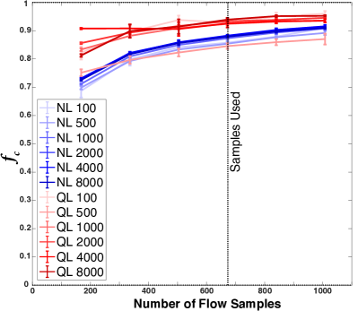
Figure 1: Basis convergence factor, $f_{c}$, for the thermal-convection case (defined in section 44.1) with a linear free surface as a function of the number of flow samples used. See (23) for the definition of $f_{c}$.

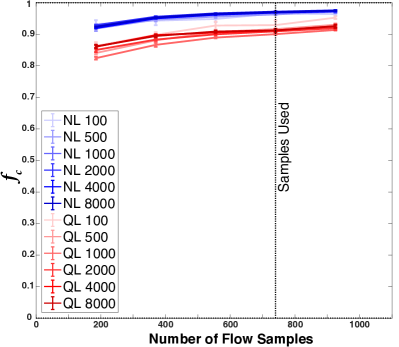
Figure 2: Basis convergence factore, $f_{c}$, for the Langmuir-turbulence case (defined in section 44.2) with a linear free surface as a function of the number of flow samples used. See (23) for the definition of $f_{c}$.

The POD modes are computed separately for each independent horizontal Fourier mode using the method of snapshots (MOS) (Holmes et al. 2012). Because the MITgcm’s pressure solver does not yield a divergenceless flow to numerical precision, flow snapshots are first projected onto a divergenceless basis to entirely eliminate the divergent modes from the decomposition. Enough flow samples are used to ensure at least 85% of the truncated basis subspace is statistically converged (see figures 1 and 2). Formally, the convergence is computed using a convergence factor, $f_{c}$, defined as the normalized inner product of the subspaces spanned by members of an ensemble of bases:

$$f_{c}=\frac{1}{N_{b}(N_{b}-1)N_{r}}\sum_{\alpha\neq\beta}\sum_{i,j}\left|\bm{\Phi}^{\alpha}_{i}\cdot\bm{\Phi}^{\beta}_{j}\right|^{2}$$ (23)

$$\bm{\Phi}^{\alpha}_{i}\cdot\bm{\Phi}^{\beta}_{j}=\tilde{\delta}_{\mathbf{m}_{i}-\mathbf{m}_{j}}\sum_{z}\Phi^{\alpha}_{i,z}\left(\Phi^{\beta}_{j,z}\right)^{*}$$ (24)

where $\bm{\Phi}^{\alpha}_{i}$ is the $i$th element of basis $\alpha$, $N_{r}$ is the number of elements in the reduced basis, and $N_{b}$ is the number of bases in the basis ensemble.

The cases studied here all involve developing turbulence and momentum as well as buoyancy entrainment in the oceanic mixed-layer. Because the statistics are not converged, samples of flow states at 21 or 37 (depending on the case) evenly spaced times are used to determine the bases. Because of this, the bases retain memory of the different states that the flow may manifest as it develops and excludes states that should not be part of the flow solution at any time. It is useful to think of the basis as encoding part of the dynamics.

3.3 Reduced-Model Implementation

This section serves as an introduction to the piece of software, Boussinesq Galerkin Projection (BGP), the reduced order model which is used in the present study and intended for use in subsequent publications. BGP is a PDE solver that discretizes symbolic equations of motion up to quadratic order, projects them onto a provided truncated basis, and integrates the resulting reduced equations explicitly forward in discrete time. The discretization is written in such a way that, when provided with a complete basis (on a necessarily very small problem), BGP will be in agreement with the MITgcm up to the precision of the latter’s pressure solver. The provided basis must be divergence-free, which allows for the reduced model to run without a pressure solver, and defined in Fourier space, which allows for easy quasilinearization of the quadratic term.

The computational complexity of BGP using a truncated basis with horizontal Fourier modes (POD) may be estimated for both the model execution and the coefficient computation (which must be computed for every unique basis and set of flow parameters) for the RNL and RQL solvers. Scaling parameters will be the number of retained modes, $N_{r}$, the number of vertical discretizations and 3D flow fields in the underlying full-basis model, $N_{zf}$, and the number of points in the stencil of the discretization of the quadratic term of the underlying full-basis model, $N_{s}$. A key assumption that will be utilized here is that the distribution function of the truncated flow representation scales linearly with $N_{r}$ such that the number of vertical modes for a given horizontal Fourier mode scales as $N_{r}^{\frac{1}{3}}$. If $N$ is the number of modes in the underlying full-basis model, then this assumption will break down as $N_{r}\rightarrow N$; however, this project is primarily concerned with model reductions of $N_{r}\ll N$. Even for $N_{r}\ll N$, the assumption may still break down if the distribution function of the truncated flow representation changes shape substantially with $N_{r}$ The following scalings are verified using runtimes from BGP in figure 3:

• the coefficient determination for RNL is $\mathcal{O}\left(N_{r}^{\frac{7}{3}}N_{zf}N_{s}^{2}\right)$

• the coefficient determination for RQL is $\mathcal{O}\left(N_{r}^{\frac{5}{3}}N_{zf}N_{s}^{2}\right)$

• the execution for RNL is $\mathcal{O}\left(N_{r}^{\frac{7}{3}}\right)$

• the execution for RQL is $\mathcal{O}\left(N_{r}^{\frac{5}{3}}\right)$

Figure 3: Runtime scalings of the reduced model (BGP) using the Langmuir-turbulence case for both the initial coefficient determination (as in equations 16 through 18) and the simulation execution. The solid and dash-dot black lines indicate the power law scalings that are predicted for the RQL and RNL.

4 Turbulence Examples

In order to investigate the feasibility and effectiveness of a quasilinear reduced model for the purpose of modeling SGS planetary turbulence, two submesoscale or smaller oceanographic flows are used as case studies: surface-forced thermal convection and Langmuir turbulence. The former case is horizontally isotropic, up to a grid-representation, while the latter is anisotropic. Crucially, both cases are formulated to be statistically horizontally homogeneous, which will permit easy computation of the mean fields and considerably simplify the POD computations and BGP execution.

The viscosity is $5000\times$ the seawater value, and the diffusivity is set equal to the viscosity (rather than less by about a factor of 7). Thus, the Kolmogorov dissipation scale is roughly $600\times$ larger for this simulation than it would be for seawater which permits representing the flows with a manageable grid and number of model, i.e., an “eddy” viscosity and diffusivity closure is used. Noting this, it should be acknowledged that the full-resolution simulations of these systems that are run on the MITgcm are not, strictly speaking, direct numerical simulations of seawater. Boundary layer problems at this resolution are more typically managed with Large-Eddy-Simulation (LES) closures (e.g., Sullivan et al. 1994), but such an approach introduces additional quadratic or higher order dependences and qualitatively similar behavior to the eddy viscosity. It is preferable, then, to maintain the linear nature of the dissipation when modeling SGS turbulent dissipation in QL dynamics.

The FNL simulation may be considered to be a type of LES despite the simple linear closure used here because the viscosity and diffusivity are much larger than the seawater values and the Prandtl number is one. LES closures generally attempt to dissipate small-scale energy while preserving the energy cascade and other dynamics present above the grid scale, when compared with a higher resolution simulation of the same flow. With QL dynamics, however, there is no energy cascade, so there can be no direct energy backscatter; rather, all energy flows through the mean field, and as long as the flow at the dissipation scales does not affect the mean-field substantially, there will not be a substantial impact at intermediate scales. Therefore, the QL flow solution is not sensitive to the relative amount of dissipation among different scales provided the net amount of dissipation is approximately preserved. There is also some flexibility in the total rate of turbulent energy dissipation because these cases are not in a steady state and the tendency of the horizontal mean-field is expected to balance much of the large-scale forcing. Roughly speaking, nonlinear LES closures tend to dissipate energy more weakly at a given scale or at smaller scales in comparison to harmonic viscosities and diffusivities, or to be flow-aware selective as to where and when large effects are needed. Here, in the FNL case, relatively weak coefficients of harmonic dissipation are used (gridscale Reynolds and Péclet numbers are $\mathcal{O}(8)$). It should be stressed, however, that the primary task here is not having an exhaustively accurate FNL simulation, but in comparing the much larger differences between the QL and NL runs and between the reduced-basis and full-basis runs–particularly with QL runs. At this level of precision, the differences between the modeling systems are much larger than differences that result from changing subgrid schemes or parameter values in the FNL run.

4.1 Thermal Convection

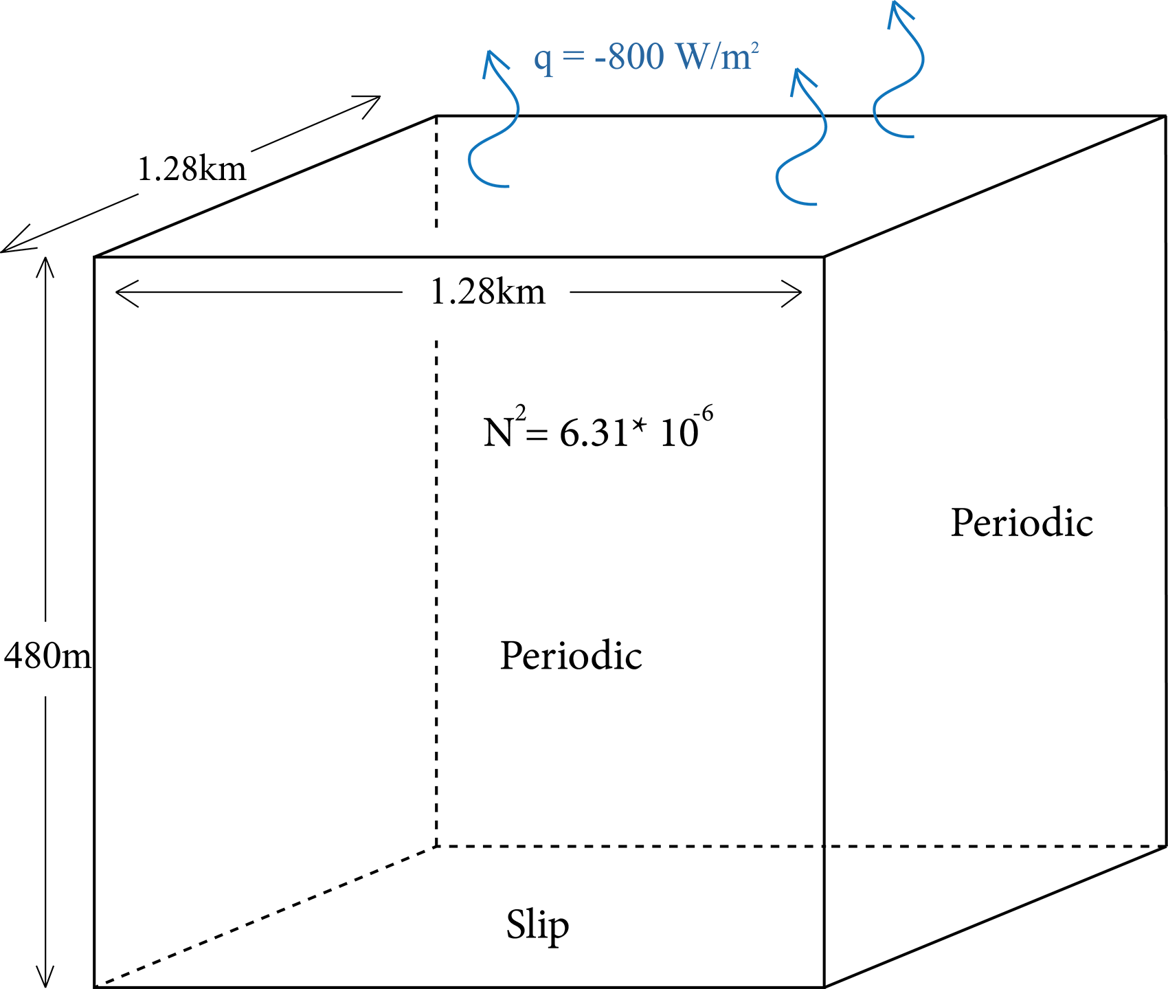
Figure 4: thermal-convection case

The surface-forced-thermal-convection case (figure 4) is formulated with an initial uniform stable stratification that is cooled from the surface (Chaalal et al. 2016). This causes the mixed layer to deepen. The nonhydrostatic Boussinesq equations that govern this case are

$$\bm{\nabla}\cdot\mathbf{u} =0$$ (25)

$$\partial_{t}\mathbf{u}+\left(\mathbf{u}\cdot\bm{\nabla}\right)\mathbf{u}+\mathbf{f}\times\mathbf{u} =-\frac{1}{\rho_{0}}\bm{\nabla}p+\mathbf{g}\alpha\left(T-T_{0}\right)$$

$$\qquad\qquad\qquad+\nu\nabla^{2}\mathbf{u}$$ (26)

$$\partial_{t}T+\left(\mathbf{u}\cdot\bm{\nabla}\right)T =\frac{Q}{c_{p}\rho_{0}}+\kappa\nabla^{2}T$$ (27)

where $\mathbf{u}=\left\{u,v,w\right\}$ is the 3-dimensional velocity vector, $T$ is the temperature field, $t$ is time, $\mathbf{f}=f\hat{\mathbf{z}}$ is the Coriolis parameter, $\rho_{0}$ is the background density, $p$ is the pressure, $\mathbf{g}=g\hat{\mathbf{z}}$ is the local acceleration of gravity, $\alpha$ is the coefficient of thermal expansion, $T_{0}$ is the background temperature, $\nu$ is the harmonic kinematic viscosity, $\kappa$ is the coefficient of thermal diffusivity, $Q$ is the volumetric heating, and $c_{p}$ is the specific heat of sea water at constant pressure. This case is defined on a regular, horizontally periodic Cartesian grid with the number of cells and grid spacing per dimension represented as $\left\{N_{x},N_{y},N_{z}\right\}$ and $\left\{\Delta_{x},\Delta_{y},\Delta_{z}\right\}$, respectively. The domain floor and surface have rigid, slip boundary conditions. In the discrete model, $Q=\delta_{k,0}\frac{q}{\Delta_{z}}$, where $k$ is the vertical layer index and $q$ is the surface heat flux.

Introducing the following non-dimensional parameters

$$Ra^{*} =\frac{g\alpha qL_{m}^{4}}{\nu\kappa^{2}\rho_{0}c_{p}}$$ (28)

$$Pr =\frac{\nu}{\kappa}$$ (29)

where $Ra^{*}$ is the modified Rayleigh Number, appropriate for a prescribed heat flux as opposed to a prescribed temperature at the boundaries, $Re$ is the Reynolds Number, $Pr$ is the Prandtl Number, and $L_{m}$ is the mixed-layer depth. Velocity and temperature scales may be introduced as in Schmidt and Schumann (1989), allowing for the definition of the Reynolds Number, a convective Froude Number, and the conventional Rayleigh Number based on a characteristic temperature difference, $T_{*}$:

$$w_{*} =\sqrt[\textrm{\small$3$}]{\frac{\alpha gqL_{m}}{c_{p}\rho_{0}}}$$ (30)

$$T_{*} =\sqrt[\textrm{\small$3$}]{\frac{q^{2}}{c_{p}^{2}\rho_{0}^{2}\alpha gL_{m}}}$$ (31)

$$Fr =\frac{w_{*}}{NL_{m}}$$ (32)

$$Ra =\frac{\alpha gT_{*}L_{m}^{3}}{\nu\kappa}$$ (33)

$$Re =\frac{w_{*}L_{m}}{\nu}$$ (34)

where $N=\sqrt{\alpha g\frac{\partial\overline{T}}{\partial z}}$ is the Brunt-Väisälä frequency, and $\overline{T}$ is the background temperature profile. Using these definitions, the case studied has the following parameters:

Figure 5: Langmuir-turbulence case

$$\left\{N_{x},N_{y},N_{z}\right\} =\left\{128,128,48\right\}$$

$$\left\{\Delta_{x},\Delta_{y},\Delta_{z}\right\} =\left\{10,10,10\right\}\textrm{m}$$

$$f =0$$

$$\rho_{0} =1035\;\textrm{kg m}^{-3}$$

$$g =9.81\;\textrm{m s}^{-2}$$

$$\alpha =2\times 10^{-4}\;\textrm{C}^{-1}$$

$$T_{0} =20\;\textrm{C}$$

$$\nu =5\times 10^{-2}\;\textrm{m}^{2}\textrm{s}^{-1}$$

$$\kappa =5\times 10^{-2}\;\textrm{m}^{2}\textrm{s}^{-1}$$

$$c_{p} =3994\;\textrm{J kg}^{-1}\textrm{C}^{-1}$$

$$q =-800\;\textrm{W m}^{-2}$$

$$N^{2} =5.45\times 10^{-7}\;\textrm{s}^{-2}$$

$$w_{*} =5.67\times 10^{-2}\;\textrm{m s}^{-1}$$

$$T_{*} =3.41\times 10^{-2}\;\textrm{C}$$

$$Ra^{*} =1.61\times 10^{8}$$

$$Ra =2.96\times 10^{5}$$

$$Pr =1$$

$$Fr =0.160$$

$$Re =544$$

Here, $N$ is the Brunt-Väisälä frequency. Using these parameters, the mixed layer depth, initially zero, will reach the bottom of the domain at approximately $t=40$ hours, at which point the execution is stopped.

4.2 Langmuir Turbulence

The Langmuir-turbulence forcing is based on McWilliams et al. (1997). The domain size and resolution have been reduced in this work, while most other case parameters are identical (see figure 5). Langmuir circulation is modeled using the phase-averaged Craik-Leibovich equations (Craik 1977). The nonhydrostatic equations governing this case are

$$\bm{\nabla}\cdot\mathbf{u}=0$$ (35)

$$\partial_{t}\mathbf{u}+\left(\mathbf{u}\cdot\bm{\nabla}\right)\mathbf{u}+\mathbf{f}\times\left(\mathbf{u}+\mathbf{{\color[rgb]{0,0,0}u_{s}}}\right)=$$

$$\qquad\qquad\qquad\qquad-\frac{1}{\rho_{0}}\bm{\nabla}\left(p+{\color[rgb]{0,0,0}\frac{\rho_{0}}{2}\left(\left|\mathbf{u}+\mathbf{u_{s}}\right|^{2}-\left|\mathbf{u}\right|^{2}\right)}\right)$$

$$\qquad\qquad\qquad\qquad+\nu_{h}\nabla_{h}^{2}\mathbf{u}+\nu_{z}\nabla_{z}^{2}\mathbf{u}$$

$$\qquad\qquad\qquad\qquad+{\color[rgb]{0,0,0}\mathbf{u_{s}}\times\bm{\nabla}\times\mathbf{u}}+{\color[rgb]{0,0,0}\frac{\bm{\tau}}{\rho_{0}}}$$

$$\qquad\qquad\qquad\qquad+\mathbf{g}\alpha\left(T-T_{0}\right)$$ (36)

$$\partial_{t}T+\left((\mathbf{u}+{\color[rgb]{0,0,0}\mathbf{u_{s}}})\cdot\bm{\nabla}\right)T=\frac{Q}{c_{p}\rho_{0}}+\kappa_{h}\nabla_{h}^{2}T+\kappa_{z}\nabla_{z}^{2}T$$ (37)

$${\color[rgb]{0,0,0}\mathbf{u_{s}}=u_{s}e^{2k_{s}z}\hat{\mathbf{x}}}$$ (38)

where $\mathbf{u}_{s}$ is the Stokes drift velocity, $\bm{\tau}=\tau\hat{\mathbf{x}}$ is the surface wind stress, $k_{s}$ is the Stokes wavenumber that sets the depth scale of the effect, $\nabla_{h}^{2}$ are the horizontal components of the vector Laplacian, $\nabla_{z}^{2}$ is the vertical component of the vector Laplacian, $\nu_{h}$ and $\nu_{z}$ are the horizontal and vertical kinematic viscosities, and $\kappa_{h}$ and $\kappa_{z}$ are the horizontal and vertical thermal diffusivities.

The parameters used for this case are

$$\left\{N_{x},N_{y},N_{z}\right\} =\left\{96,96,72\right\}$$

$$\left\{\Delta_{x},\Delta_{y},\Delta_{z}\right\} =\left\{3,3,0.9\right\}\;\textrm{m}$$

$$f =1\times 10^{-4}\;\textrm{s}^{-1}$$

$$\rho_{0} =1035\;\textrm{kg m}^{-3}$$

$$g =9.81\;\textrm{m s}^{-2}$$

$$\alpha =2\times 10^{-4}\;\textrm{C}^{-1}$$

$$T_{0} =20\;\textrm{C}$$

$$\nu_{h} =2\times 10^{-3}\;\textrm{m}^{2}\textrm{s}^{-1}$$

$$\kappa_{h} =2\times 10^{-3}\;\textrm{m}^{2}\textrm{s}^{-1}$$

$$\nu_{z} =1\times 10^{-3}\;\textrm{m}^{2}\textrm{s}^{-1}$$

$$\kappa_{z} =1\times 10^{-3}\;\textrm{m}^{2}\textrm{s}^{-1}$$

$$c_{p} =3994\;\textrm{J kg}^{-1}\textrm{C}^{-1}$$

$$q =-5\;\textrm{W m}^{-2}$$

$$N^{2} =1.936\times 10^{-5}\;\textrm{s}^{-2}$$

$$\tau =0.037\;\textrm{N m}^{-2}$$

$$u_{s} =0.068\;\textrm{m s}^{-1}$$

$$k_{s} =0.105\;\textrm{m}^{-1}$$

$$L_{m} =32.1\;\textrm{m}$$

$$u_{*} =6.0\times 10^{-3}\;\textrm{m}\textrm{s}^{-1}$$

$$Re_{*} =191.9$$

$$La =0.2965$$

Here, $L_{m}$ is the initial mixed-layer depth, above which the fluid temperature is initially uniform, $u_{*}=\tau^{\frac{1}{2}}\rho_{0}^{\frac{1}{2}}$ is the friction velocity, Re${}_{*}=\frac{u_{*}L_{m}}{\nu_{z}}$ and the Langmuir number is defined as

$$La=\sqrt{\frac{\tau^{\frac{1}{2}}}{\rho_{0}^{\frac{1}{2}}u_{s}}}$$ (39)

The surface cooling is included for consistency with McWilliams et al. (1997) where it is used to help destabilize the flow; it does not have a significant impact on the dynamics otherwise, so the Rayleigh and Prandtl number are not important. The simulation is stopped at 72 hours.

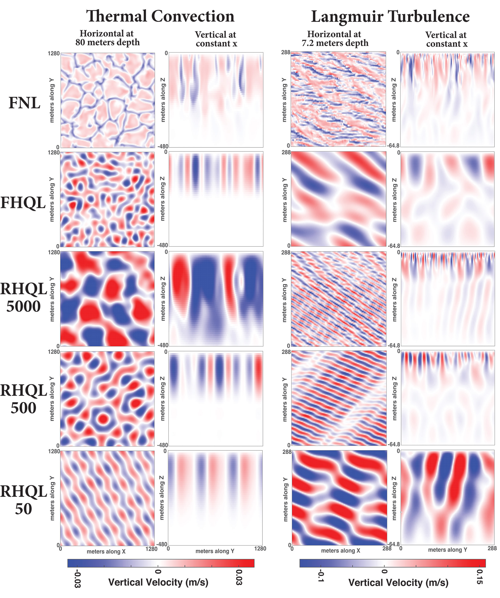
Figure 6: Cross-sections of vertical velocity fields from an ensemble member of the thermal-convection case at $t=10$ hours and from an ensemble member of the Langmuir-turbulence case at $t=54$ hours. Horizontal cross sections (top half of figure) are at 80 meters depth in the thermal convection case and 7.2 meters depth in the Langmuir case. By incompressibility, $\overline{w}=0$, so $w=w^{\prime}$.

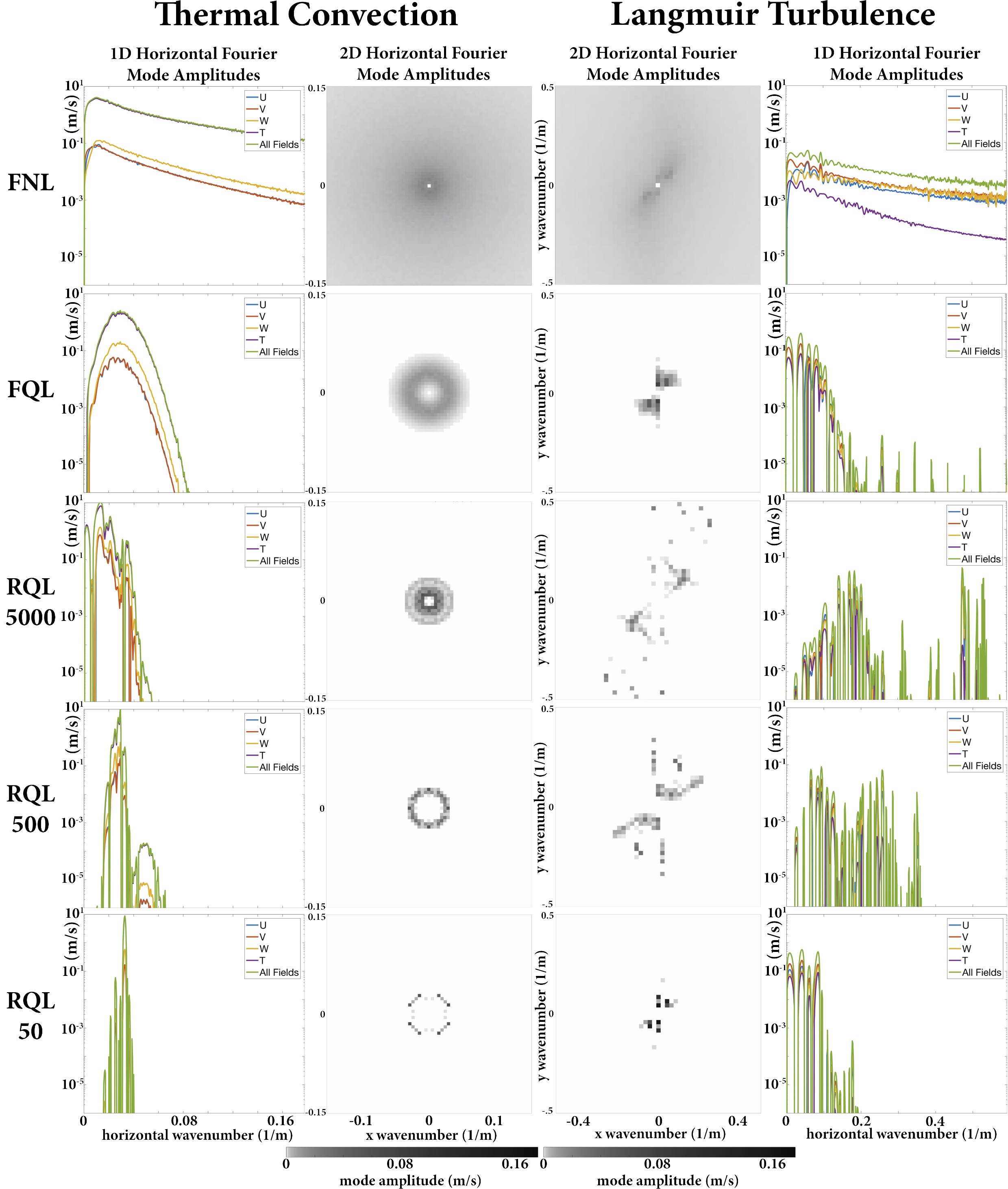
Figure 7: Center columns: The 2D horizontal mode amplitude of the thermal-convection fields at 20 hours and the Langmuir-turbulence fields at 54 hours for different types of dynamics and basis sizes. These are computed from an ensemble average of 12 reduced-model fields and 24 full-basis fields. The wavenumber axes show half of the modes accessible in the full-basis representation. Outer columns: The 1D horizontal mode amplitudes at the same times. Temperature is scaled as described in section 33.2.

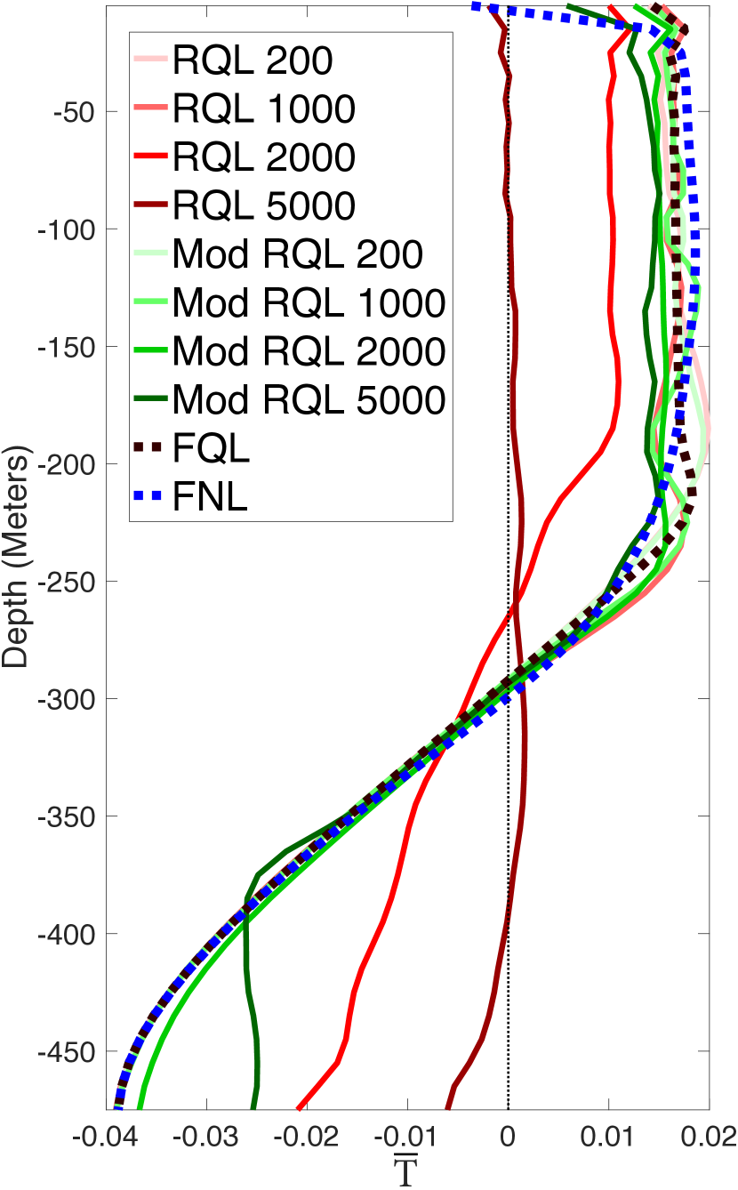
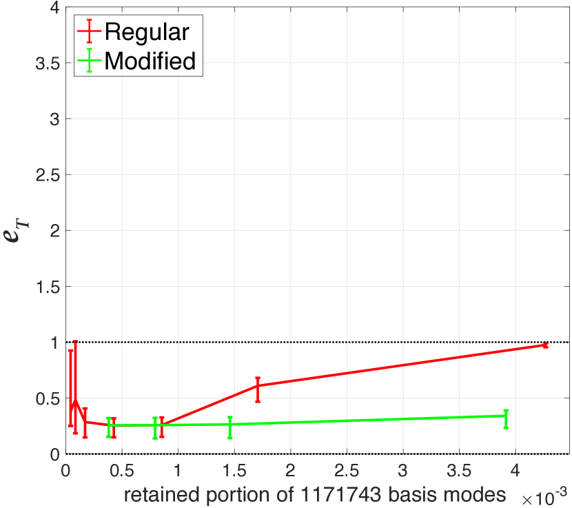
(a) Thermal Convection

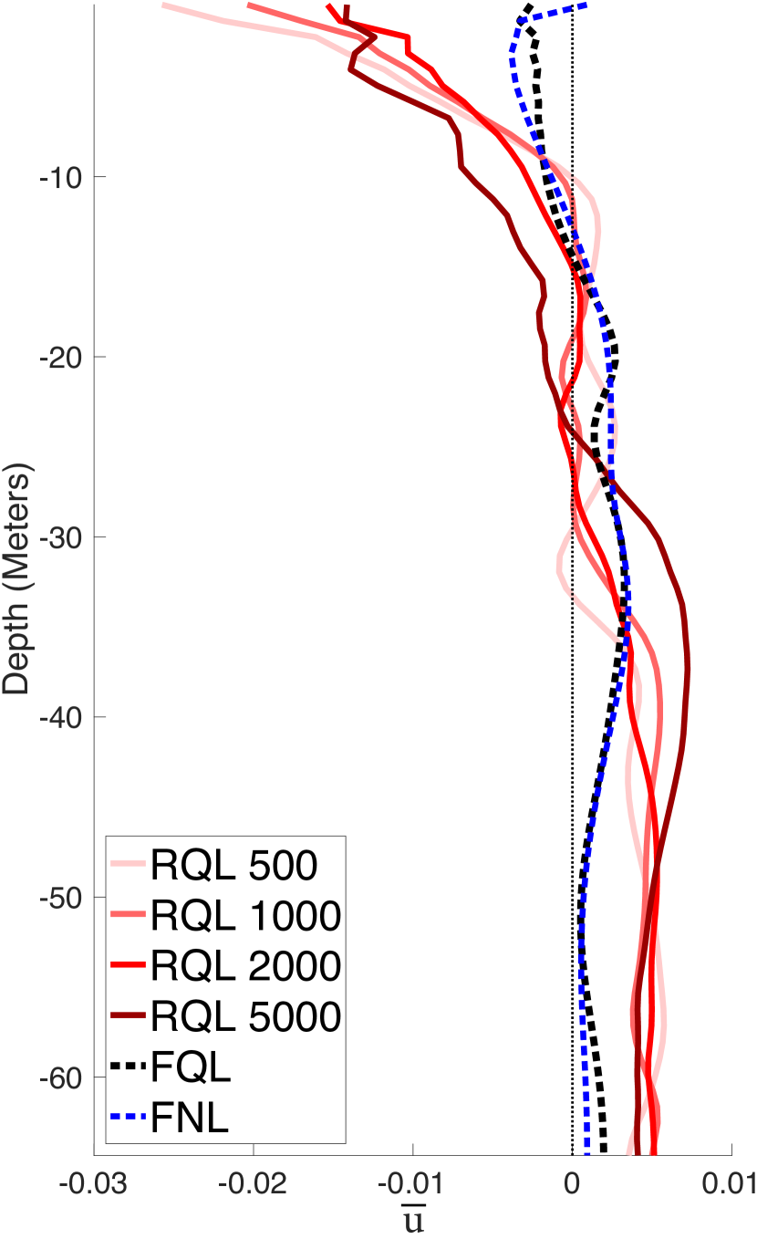
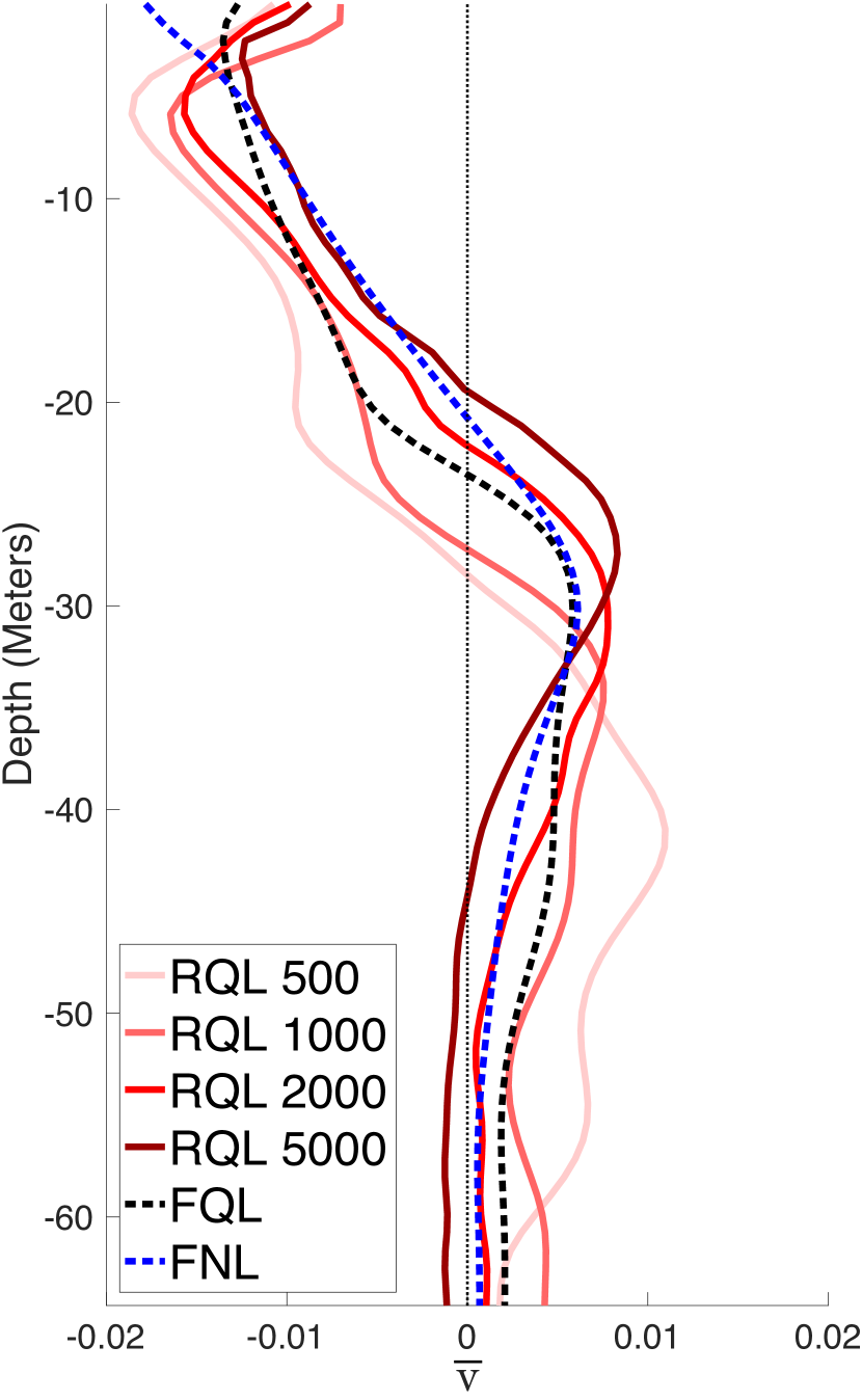
(b) Langmuir Turbulence

width 2pt

Figure 9: Top Row: Ensemble-averaged mean-field vertical profiles for the thermal-convection case at $t=10$ hours and for the Langmuir-turbulence case at $t=18$ hours. Bottom Row: error of ensemble averaged mean-field profiles as a function of truncated basis size, as defined in equation 40. For the thermal-convection profiles, both the regular 5000-mode truncated POD basis and a modified version omitting some large-scale horizontal modes (defined in section 55.4 and depicted in figure 13) are shown.

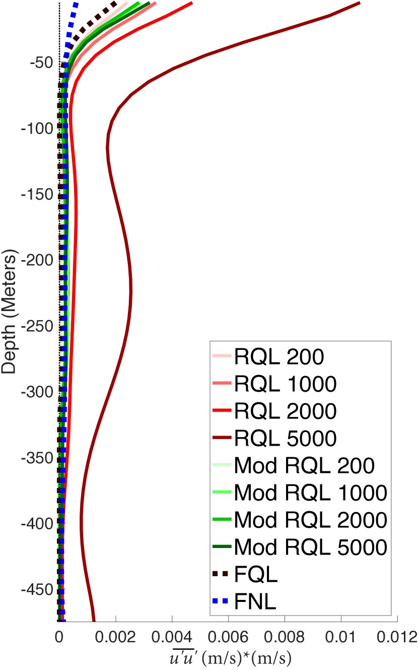
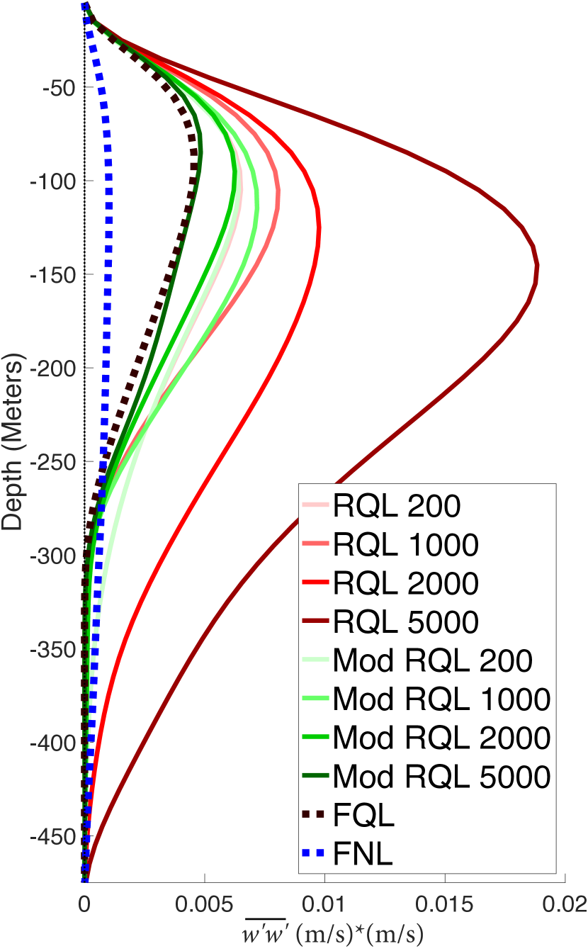
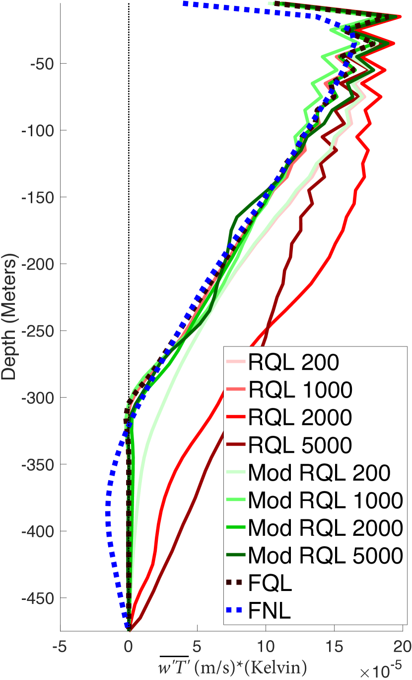
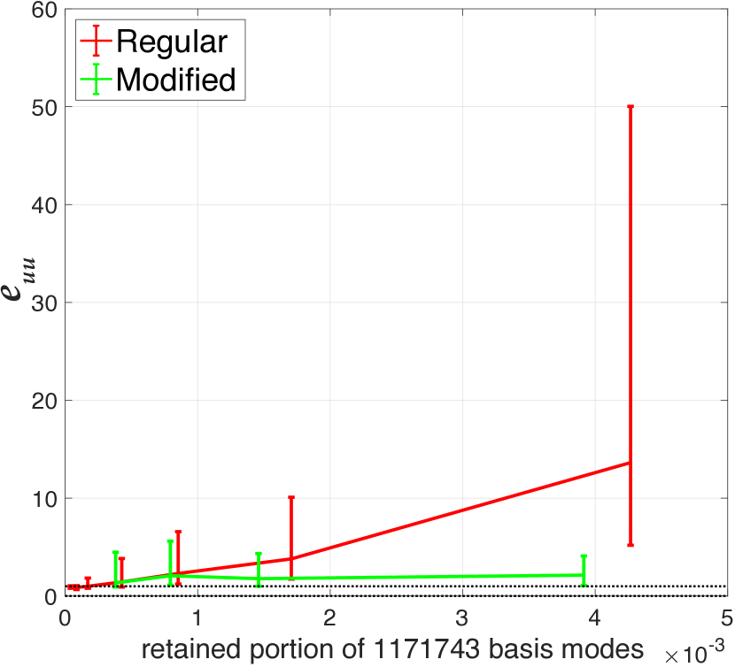
(a) $\overline{u^{\prime}u^{\prime}}$

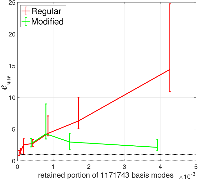
(b) $\overline{w^{\prime}w^{\prime}}$

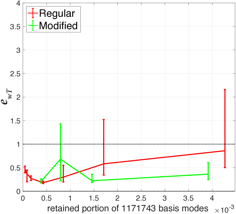
(c) $\overline{w^{\prime}T^{\prime}}$

Figure 10: Top Row: Vertical profiles of turbulent transports and energies of the thermal-convection cases at $t=20$ hours. Bottom Row: Vertical-profile error, $e_{ij}$, defined in equation 41, vs retained basis size for different statistical profiles of the thermal-convection cases. The modified version of the truncated bases is defined in section 55.4 and depicted in figure 13. Note that $e_{ij}$ accounts for the profiles that are evenly sampled throughout the flow evolution. Although there must be a general trend for the RQL statistical profiles to converge on the FQL profiles, this convergence will not generally be uniform, as is seen in the poor representation of the 5000-mode profiles in particular. Convergence properties will be explored more thoroughly in section 55.5.

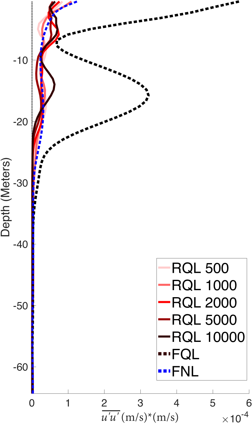
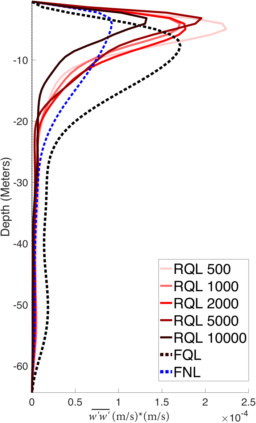
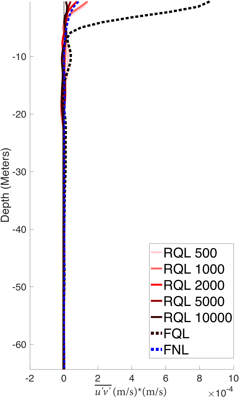
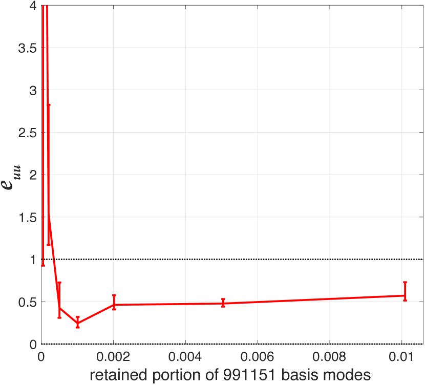
(a) $\overline{u^{\prime}u^{\prime}}$

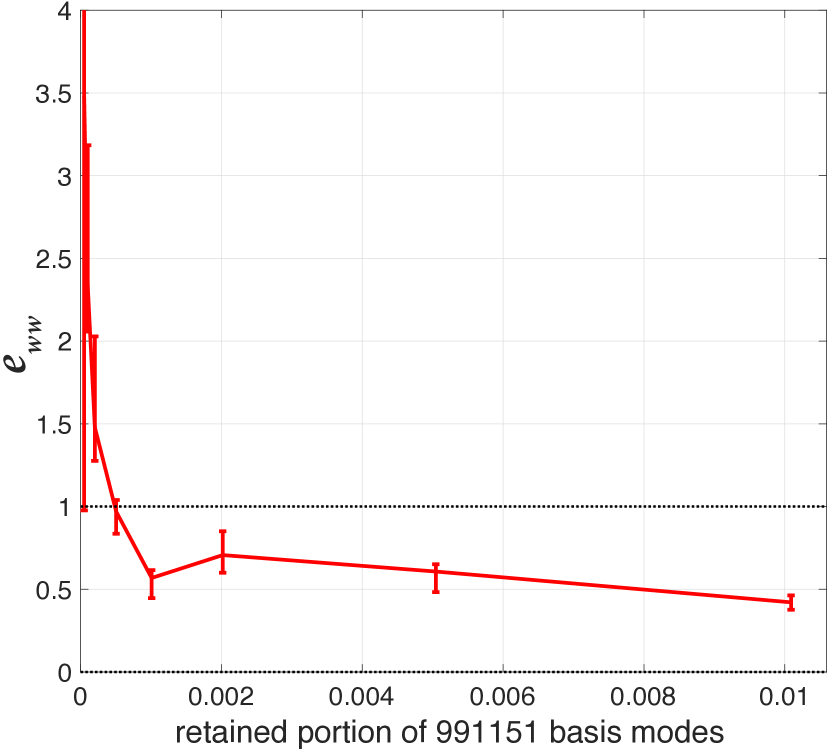
(b) $\overline{w^{\prime}w^{\prime}}$

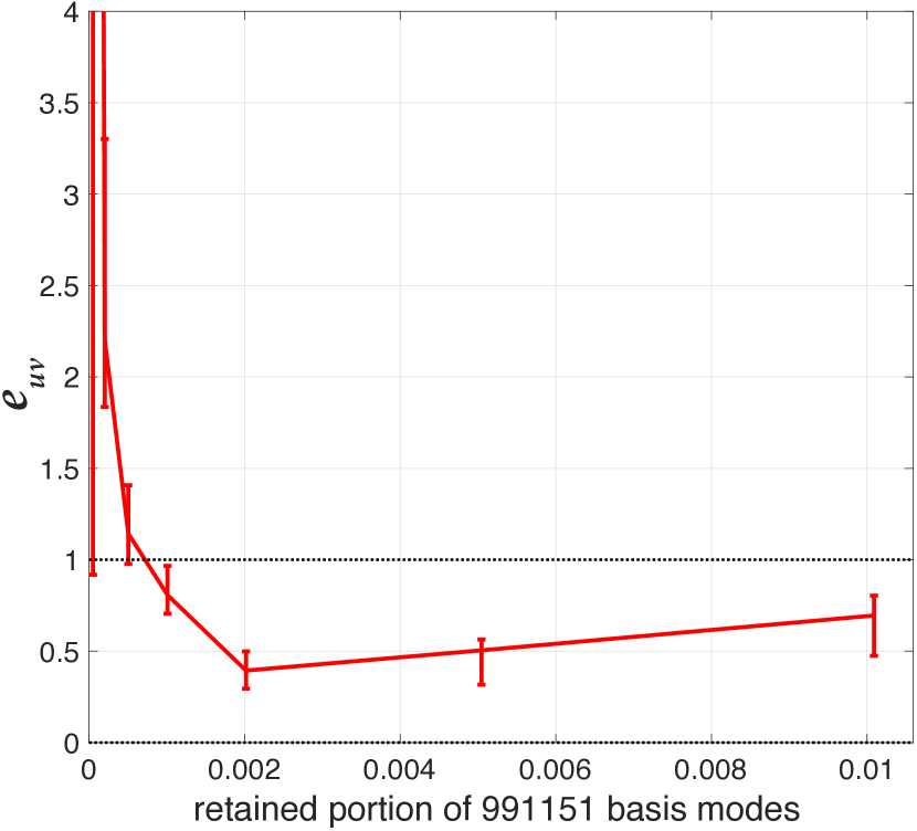
(c) $\overline{u^{\prime}v^{\prime}}$

Figure 11: Top Row: Vertical profiles of turbulent transports and energies of the Langmuir-turbulence cases at $t=36$ hours. Bottom Row: Vertical-profile error, $e_{ij}$, defined in equation 41, vs retained basis size for different statistical profiles of the Langmuir-turbulence cases. Note that $e_{ij}$ accounts for the profiles that are evenly sampled throughout the flow evolution.

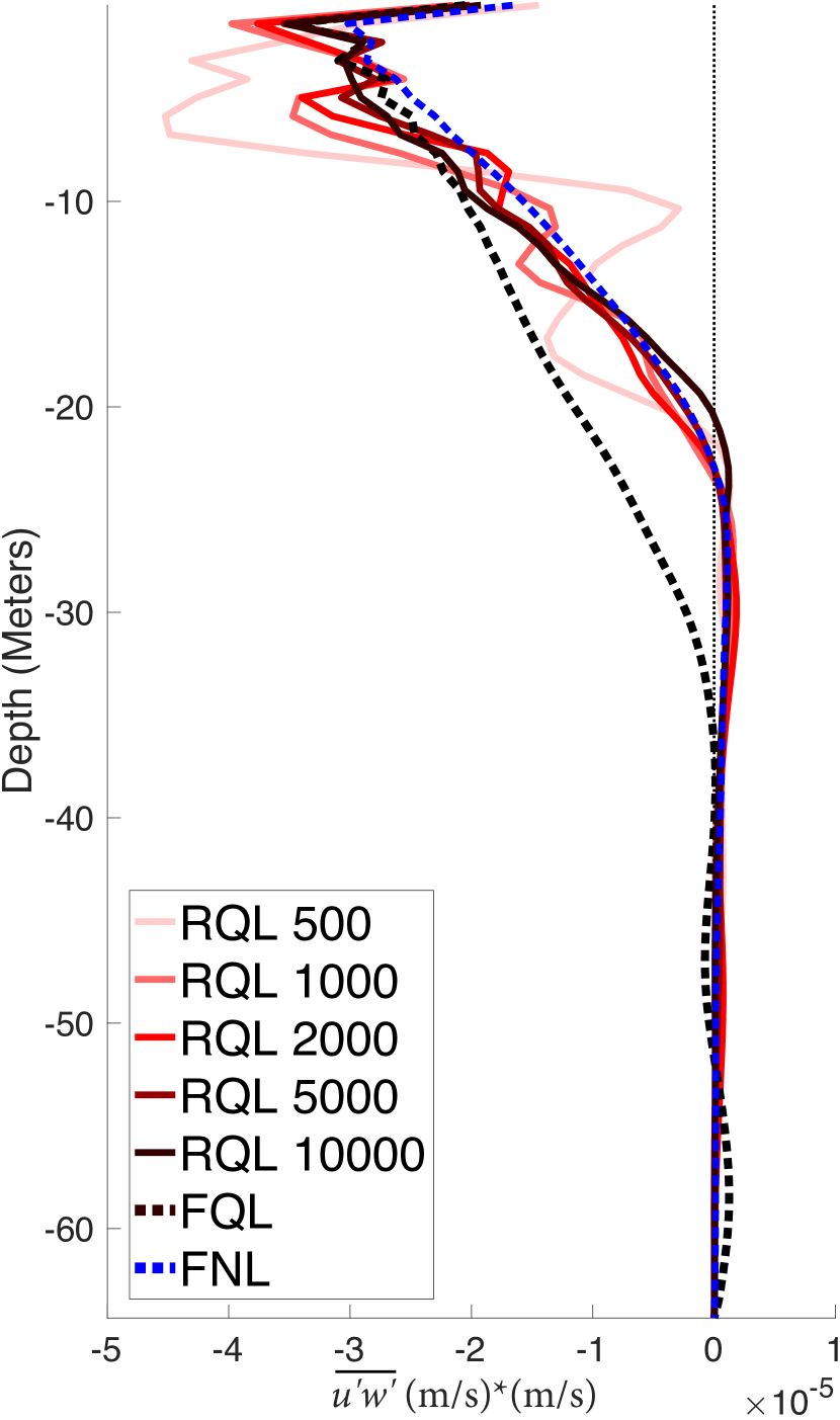
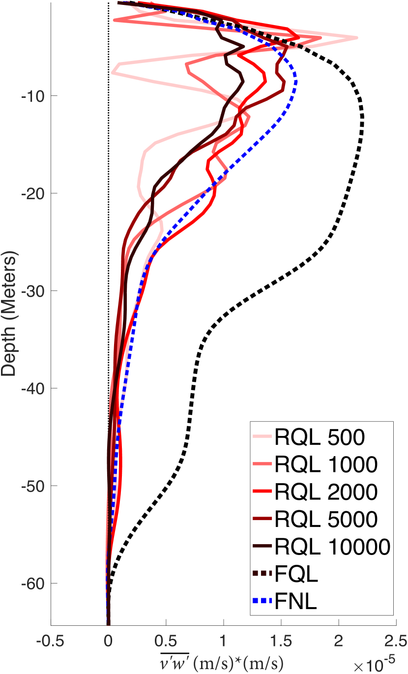
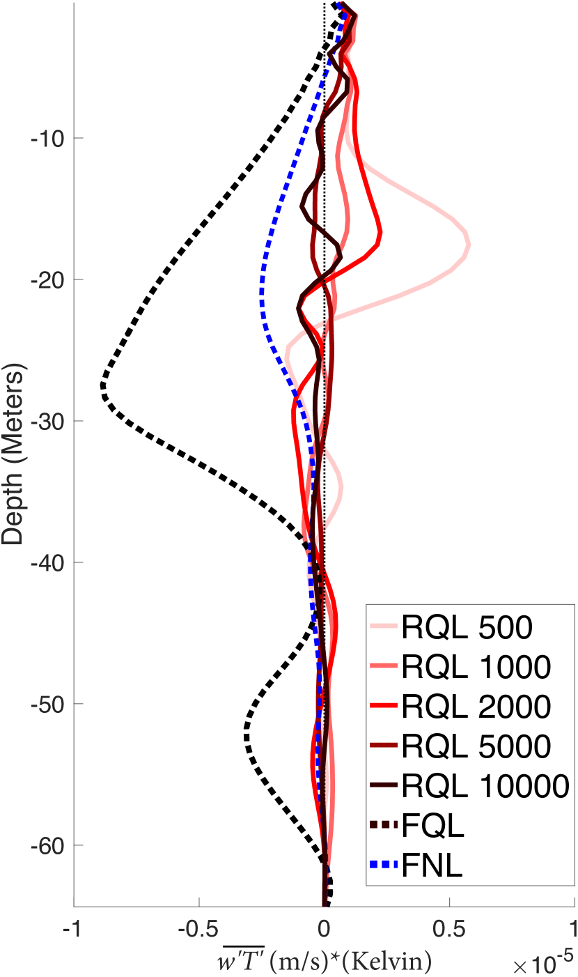
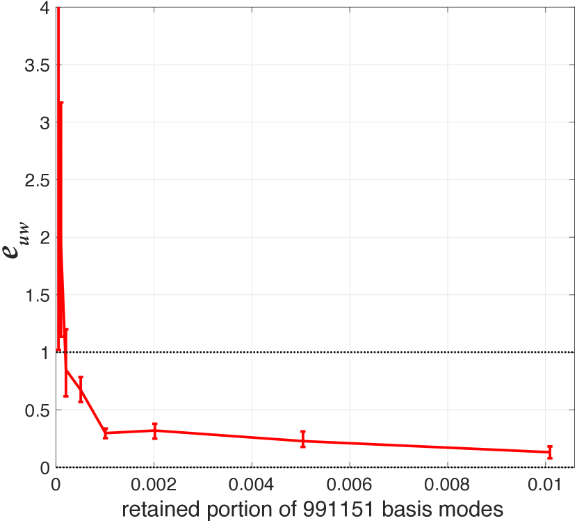
(a) $\overline{u^{\prime}w^{\prime}}$

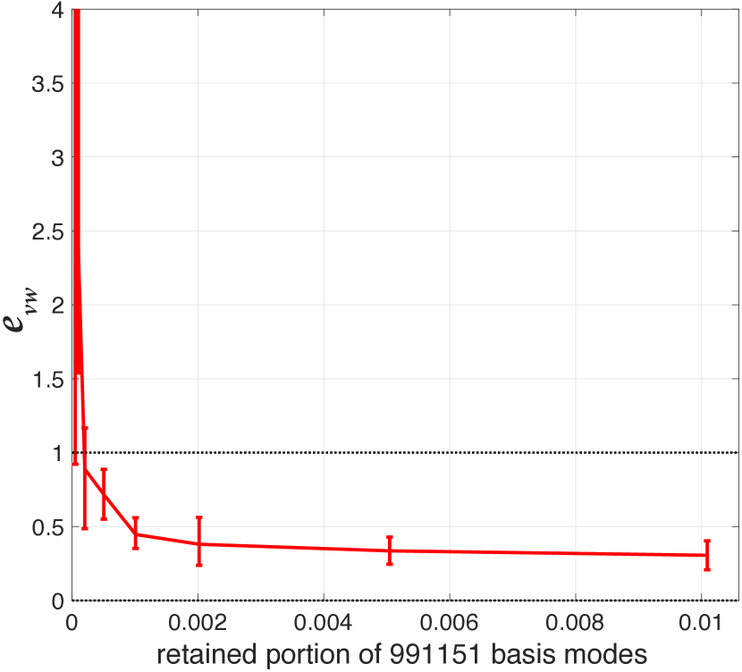
(b) $\overline{v^{\prime}w^{\prime}}$

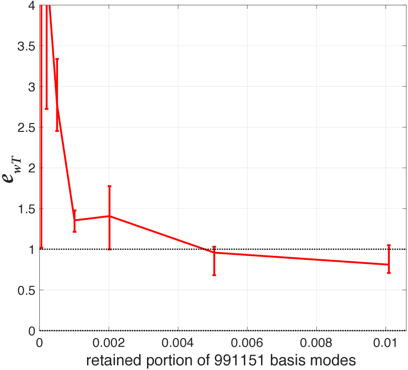
(c) $\overline{w^{\prime}T^{\prime}}$

Figure 12: Top Row: Vertical profiles of turbulent transports and energies of the Langmuir-turbulence cases at $t=36$ hours. Bottom Row: Vertical-profile error, $e_{ij}$, defined in equation 41, vs retained basis size for different statistical profiles of the Langmuir-turbulence cases. Note that $e_{ij}$ accounts for the profiles that are evenly sampled throughout the flow evolution.

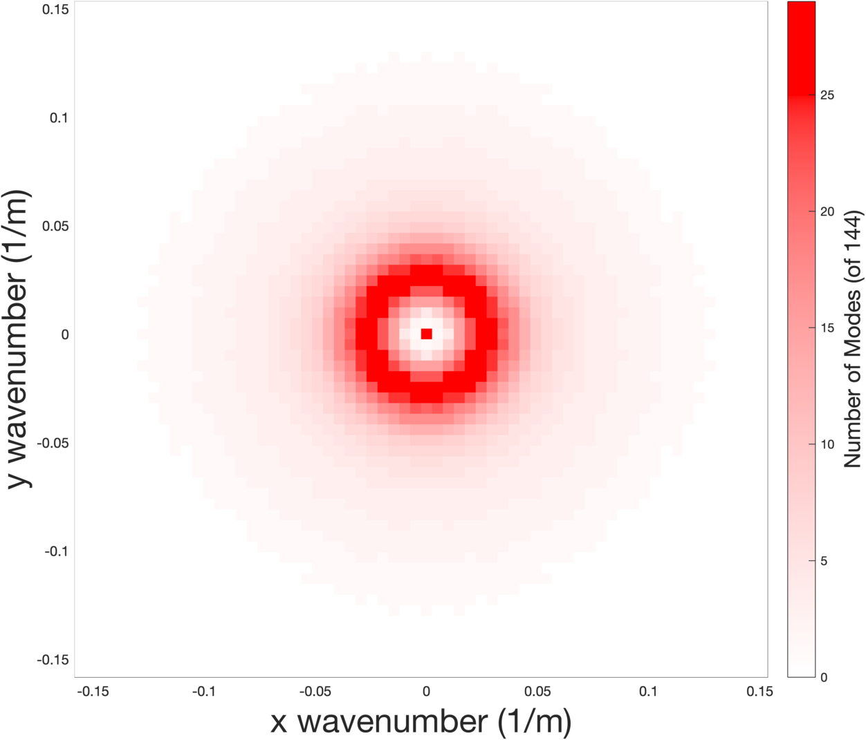
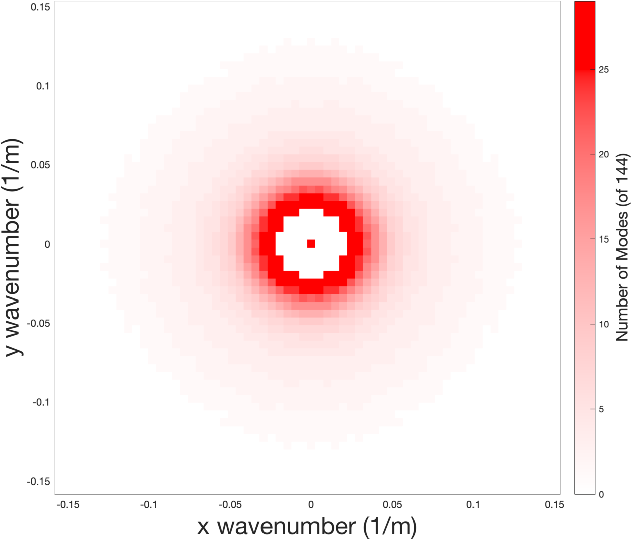
Figure 13: The horizontal Fourier mode density within the 5000-mode truncated basis: (left) the regular POD truncation (right) the "modified" version of this basis in which horizontal Fourier modes with less than 85% of the peak representation mode and with larger horizontal scales than that mode are omitted. The omitted large-scale modes are associated with plumes that extend beyond the mixed-layer early in the flow evolution.

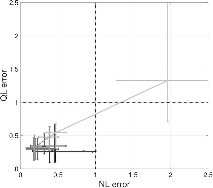
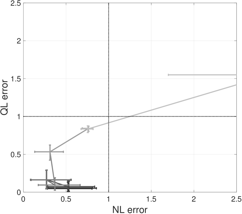
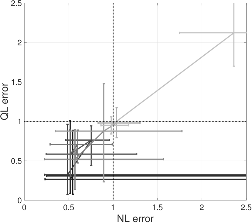
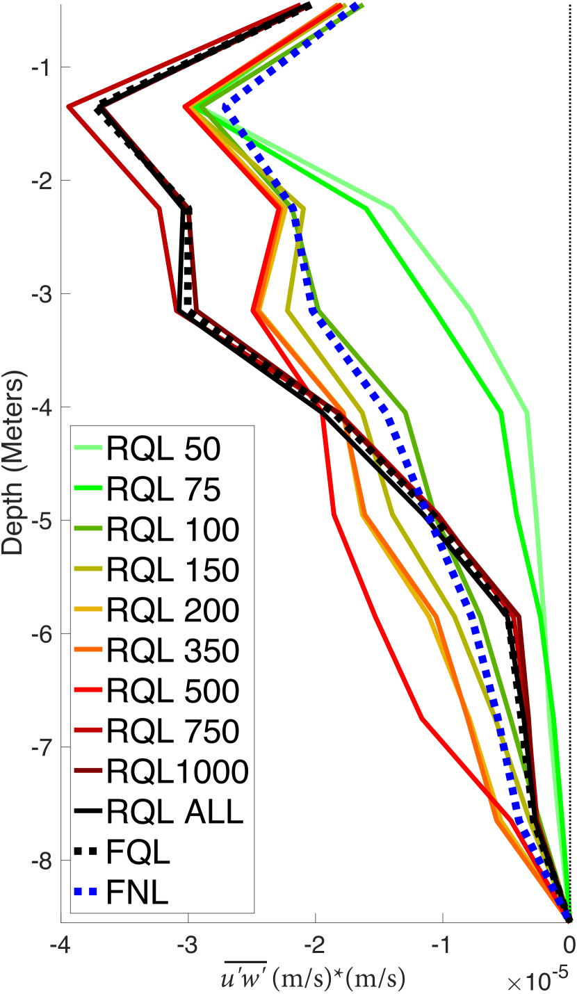
(a) $\overline{u^{\prime}w^{\prime}}$

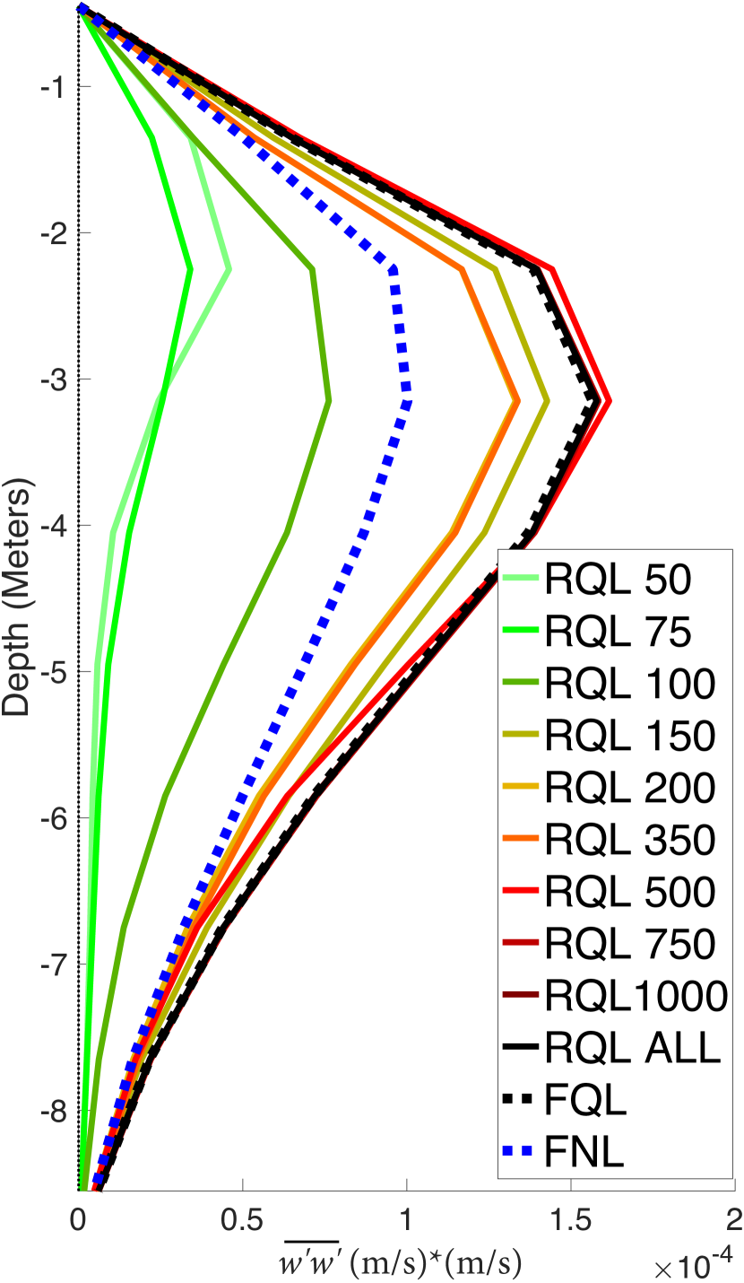
(b) $\overline{w^{\prime}w^{\prime}}$

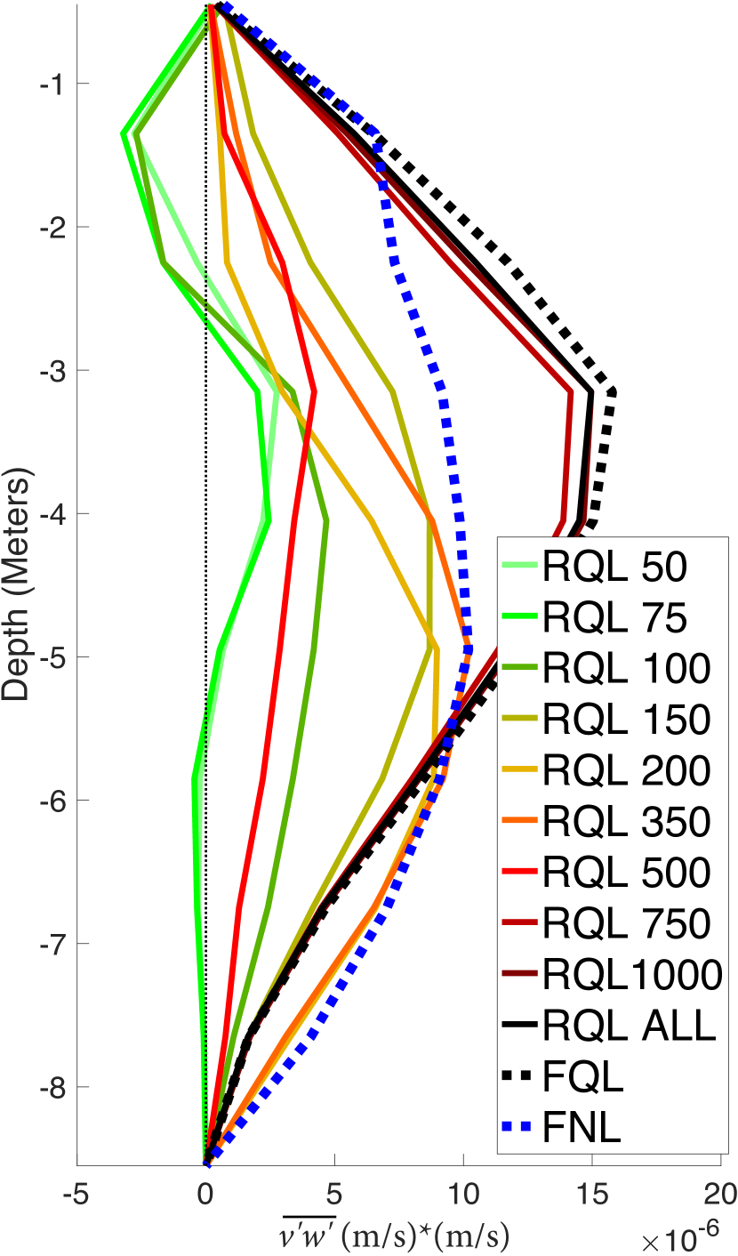
(c) $\overline{v^{\prime}w^{\prime}}$

Figure 14: For a 10 $\times$ 10 $\times$ 10 miniature version of the Langmuir-turbulence model. Top Row: error of RQL turbulent transport and energy vertical profiles in representing FNL vs FQL profiles. Darker lines indicate greater basis retention, with black being complete representation. Bottom Row: turbulent statistical profiles as a function of depth for different truncated basis sizes. Some of the RQL turbulent profiles, such as $\overline{u^{\prime}w^{\prime}}$ after 120 minutes of flow evolution, are more representative of FNL than FQL, something observed in the larger Langmuir-turbulence case at incomplete basis representation (see figures 11 and 12.) Other RQL turbulent transports and energies, such as $\overline{w^{\prime}w^{\prime}}$ at 90 minutes, sweep through the space of accessible profiles and appear to represent the FNL profiles well at certain retention rates seemingly by chance. Finally, other RQL statistical profiles, such as $\overline{v^{\prime}w^{\prime}}$ at 120 minutes, do not approximate the FNL profiles better than the FQL profiles at any basis size.

5 Results

5.1 Full-Basis Results

Figure 6 shows horizontal cross sections of specific instances of the vertical velocity field of both the thermal-convection case (TC) and the Langmuir-turbulence case (LT) for FNL, FQL, and various truncations of RQL. Figure 7 compliments this with ensemble-averaged horizontal Fourier spectra of the flow fields taken at the same times. The full-basis results in the top two rows of these figures will first be addressed.

For TC vertical-velocity fields (top-left of figure 6), FQL has different horizontal scales and shapes than FNL. FNL has geometric patterns of upwelling delineated by relatively intense, spoke-like plumes. FQL, on the other hand, has very regular, horizontally wave-like plumes that are almost homogeneous in the vertical direction within the mixed layer. The amplitude of the velocities is also observed to be substantially exaggerated in the FQL case. Additionally, there is an apparent sign-reversal symmetry within the vertical velocity field of FQL. This is because the Fourier modes have phases that are independent of one another, as described in section 2. For a given wavenumber amplitude, there are many such independent Fourier modes on or near an annulus in wavenumber space of that radius; these must be approximately equally excited due to horizontal isotropy, creating an apparent sign-inversion symmetry within a single snapshot of the flow.

For LT FNL vertical-velocity fields (top-right of figure 6), alternating bands of upwelling and downwelling are observed, broken up by small-scale turbulent features. Like with TC, although less noticeably, the downwelling part of the structures are narrower and more concentrated. The rolls have been rotated away from the direction of the wind and waves by the Coriolis force; the angle of rotation is dependent on depth. FQL looks a bit like it could be a filtered version of the FNL solution (unlike TC); however, again, there is an apparent sign-inversion symmetry that is not present in FNL. As with TC, the vertical velocity field is overly strong, likely due to a lack of small-scale turbulence acting on the primary instability.

The Fourier spectra in the top two rows of figure 7 reveal that in FQL, for both cases, the modes that are populated are near those which are the most energetic in FNL. Outside of this concentrated region of wavenumbers the energy falloff is steep. This reflects the lack of a cascade to spectrally local modes.

The top row of figure 9 shows vertical profiles of horizontal and ensemble-averaged mean fields for FNL and FQL, (as well as several truncations of RQL, to be discussed in section 55.3). FQL is able to reproduce the FNL fairly well. The horizontal mean fields are particularly important in the quasilinear approximation as they are the only way turbulent energy can move among horizontal Fourier modes, so it is expected that the rough agreement between FQL and FNL mean profiles is an important foundation for making further approximations in the form of model reduction.

In contrast to the mean-field profiles (figure 9), the second-order FQL profiles (figures 10, 11, and 12) generally do not exhibit good agreement with the FNL profiles. For the thermal-convection case, the only nonlinear profile that is well represented by FQL is the vertical turbulent temperature transport, $\overline{w^{\prime}T^{\prime}}$, figure 10(c). This is likely because the transport of temperature is what is driving the flow; a mean-field temperature anomaly builds at the surface due to the prescribed heat flux and is preferentially transported downwards due to the eddy field. This term dominates the turbulent-kinetic-energy production, which is also accurately represented although not depicted. Note that other off-diagonal Reynolds stresses are exactly zero in the limit of a large ensemble average because of the horizontal isotropy of this case, so there are relatively few non-trivial second-order vertical statistical profiles to observe in TC. For LT, none of the second-order FQL profiles are well-represented.

5.2 Reduced-Model Fields and Spectra

Reduced-basis fields and horizontal Fourier spectra for TC and LT are provided in figures 6 and 7, respectively, along with those of the full bases. At a glance, the behavior of TC and LT are substantially different under the model reduction. In the former case, modes are populated at slightly smaller wavenumbers than FQL while in LT at truncations larger than 50, energy tends to be in much larger wavenumbers than FQL. The RQL flow solution and statistics must eventually converge upon those of FQL as the basis size is further increased. The convergence of the Fourier energy footprint is therefore nonuniform, where smaller basis retentions can actually look more like FQL than the larger basis retentions. It will turn out to be the case that this nonuniform convergence can be advantageous in that it allows for better representation of the FNL statistical profiles. The nonuniform convergence of the RQL flow statistics on those of FQL is explored more thoroughly in a small test case in section 55.5.

In TC RQL 50, the observed rows of plumes are due to an insufficient number of retained eddy-modes on the dominant wavenumber (see bottom left of figure 7). The basis was selected in a manner that observes discrete horizontal isotropy exactly, so the non-zero modes show an eight-fold symmetry; however, with fifty modes, the truncation is so severe that the annulus is not complete and modes along the axes are omitted. Because so few modes are excitable near this wavenumber, their amplitudes do not average out to form smooth structures that reflect the symmetry of the problem, rather, one or two may randomly dominate at a given time, giving rise in some instances to rows, in others to regular triangular patterns. Despite the qualitative shortcomings, the vertical profile resembles the FQL solution, exaggerating the plume depth slightly. In LT RQL 50, the breaking of horizontal isotropy allows for 50 modes to better capture the essential shape of the windrows than with TC; however, the velocity field is too strong and penetrates through the stratified layer.

At 500 modes, both TC and LT show improvement in the vertical cross sections of the flow fields (figure 6), a reflection of the larger number of accessible modes, as seen in the 2D Fourier spectrum in figure 7. The horizontal cross sections of both cases reflect RQL’s shift to different horizontal scales compared with FQL; in TC RQL 500, the solution has similar horizontal structure as FQL except with slightly larger length scales, while in LT RQL 500, the windrows are much more narrow. This trend is more pronounced at 5000 modes. The displacement of the excitation of horizontal Fourier modes at intermediate basis truncations in RQL is explored more thoroughly in section 55.4.

5.3 Reduced-Model Statistical Profiles

The mean-field profiles are depicted in figure 9 along with their representation error:

$$e_{i}=\frac{\left(\left<\overline{q}_{i,FNL}\right>-\left<\overline{q}_{i,RQL}\right>\right)\cdot\left<\overline{q}_{i,FNL}\right>}{\left<\overline{q}_{i,FNL}\right>\cdot\left<\overline{q}_{i,FNL}\right>}$$ (40)

Here, the mean field is $\left<\overline{q}\left(z,t\right)\right>$, $\left<\right>$ indicates an ensemble average, the subscript runs over the fields $\left\{u,v,w,T\right\}$, $t$ runs over four evenly sampled times throughout the flow evolution, $z$ runs over the vertical position, and the dot product is defined over both $z$ and $t$. The top-rows of figures 10, 11, and 12 depict vertical profiles of horizontal and ensemble averaged turbulent transports and energy terms, while the bottom rows show the RQL model’s representation error, $e_{ij}$ of the FNL statistical profiles, computed as a normalized inner product of the Reynolds stresses $\left<\overline{q_{i}q_{j}}\right>=\bm{\tau}_{ij}=\tau_{ij}\left(z,t\right)$:

$$e_{ij}=\frac{\left(\bm{\tau}_{ij,FNL}-\bm{\tau}_{ij,RQL}\right)\cdot\bm{\tau}_{ij,FNL}}{\bm{\tau}_{ij,FNL}\cdot\bm{\tau}_{ij,FNL}}$$ (41)

Note that errors less than $0.3$ usually indicate a good qualitative representation of the vertical profile.

At small basis sizes (200 and 1000), the mean-field thermal-convection temperature profile, depicted on the left of figure 9(a), as well as the vertical temperature transport, $\overline{w^{\prime}T^{\prime}}$ (right of figure 10), are represented well by RQL. At 5000 modes, however, unrealistically strong and deep profiles of $\overline{w^{\prime}w^{\prime}}$ and $\overline{w^{\prime}T^{\prime}}$ in figures 10(b) and 10(c), respectively, have mixed the domain entirely by the time of 20 hours, demonstrating a deviation from uniform convergence towards the FQL statistics. An explanation and solution for this anomalous mixing using a modified POD basis is given in section 55.4.

Unlike the thermal-convection case, the Langmuir-case momentum mean field profiles in figure 9(b) do not exhibit a trend of worse representation at larger basis sizes. The FQL $v$-velocity profile appears qualitatively consistent with the FNL profiles; however, the $u$-velocity component exhibits errors on the order of the magnitude of the FNL mean field (meaning $e_{u}\approx 1$). Note that for none of the mean-field profiles does RQL outperform FQL at reproducing the FNL mean fields. This may be unsurprising given the degree of reduction of the model size; however, it will turn out that RQL will sometimes perform better than FQL for second-order profiles.

The Langmuir-turbulence case, on the other hand, exhibits good representation of several turbulent transport and energy profiles with RQL; however, it requires a larger portion of retained basis modes to do this, about $0.2\%$ of modes, or about a factor of 10 more than the thermal-convection case. Several of the RQL turbulent transport and energy profiles (specifically $\overline{u^{\prime}u^{\prime}}$, $\overline{w^{\prime}w^{\prime}}$, $\overline{u^{\prime}v^{\prime}}$ and $\overline{v^{\prime}w^{\prime}}$), appear to initially converge on the FNL profiles (as opposed to FQL), something which was not observed in the mean-field profiles in figure 9. The potential of RQL to reproduce second-order FNL statistics would be a huge boon to sub-grid-scale modeling within the ocean-surface boundary layer, so the mechanism for this convergence is scrutinized in section 55.4. It can also be noted that the relatively good performance of RQL at reproducing second-order FNL profiles compared with first-order mean profiles indicates the mean fields may not be as essential as would have been expected given their important role as an energy pathway in the quasilinear approximation.

5.4 Reduced Basis Excitation Displacement

In order to understand the convergence of RQL on FNL statistics in LT as well as the degradation of performance of RQL TC at intermediate basis truncations, it is helpful to first identify the cause and impact of the change in excited horizontal Fourier wavenumbers that occurs in RQL relative to FQL (see figure 7). Recall that relative to FQL, RQL 5000 prefers smaller wavenumbers in TC and quite a bit larger in LT. To probe the mechanism for this spectral excitation displacement, simulations were run to determine the growth rate of quasilinear instabilities around a fixed FQL mean field for different basis truncations. Based on these numerical experiments, the peak quasilinear instability is displaced to different horizontal scales because the truncation of these excited horizontal modes prevents the redistribution of energy to different vertical profiles within that horizontal mode. This then prevents the draining of energy that would otherwise occur in the full-basis solution. In the LT fixed-mean-field experiments, high-wavenumber modes are driven by the linear Stokes instability. In the full-basis flow solution, the vertical profile of this mode evolves through an interaction with the mean field, and backscatter and vertical viscosity both act to dissipate this energy such that the mode never becomes substantially energized. In the 5000-mode version, however, the representation of these horizontal Fourier modes is limited and energy is not able to vertically redistribute in order to drain through these mechanisms. Similarly, in TC the smaller-wavenumber modes are excited via scattering off of the mean field and efficiently dissipated via backscatter, viscosity, and thermal diffusion in the full-basis solution, with the truncated basis (1000+) suppressing this pathway.

Having identified the cause of these shifted peak excitations to be an insufficient representation of the associated horizontal Fourier modes, next consider their impact on the mean-field and vertical structure of the flow. Recall that the POD bases are computed using snapshots of FQL flow solutions. In FQL, boundary layer structures are simple, spectrally focused, and uniform throughout the mixed layer (relative to FNL). The horizontal dimension of these flow structures scales monotonically with the mixed-layer depth. When the basis truncation of a horizontal Fourier mode is very limited, such as at the horizontal wavenumbers of the displaced peak excitations in LT and TC, the included vertical modes will allow for only a small variation of mixed-layer depths around the preferred depth of the original FQL solution. Because of this, in LT the displaced peak-excitation Fourier modes of a high-wavenumber create structures of a shallower profile than the overall MLD (which is controlled by some of the less energetic and smaller wavenumber modes). The interior of the mixed layer becomes structurally less homogeneous, and therefore more FNL-like (bottom-right of figure 6). For TC, the displaced peak-excitation horizontal Fourier modes artificially push the mixed-layer beyond its correct size, causing the RQL profiles to be a much worse representation of the FQL results (Fig. 10).

The reason that TC and not LT exhibits displaced mode excitation at larger scales is because in TC the representation of small-wavenumber modes gradually trails off at small wavenumbers in the FQL solution while for LT they are continuously represented up to a sharp cutoff, missing only a single discrete wavenumber next to the mean field (see figure 7.) A means of addressing the inaccuracies associated with large-scale displaced RQL mode excitation while preserving the benefits of the small-scale modes is to allow the reduced-basis solver to use only those partially represented modes that are approximately of equal or larger horizontal wavenumber than the peak excitations. This basis modification could be efficient to implement because it can take effect at runtime, which stands in contrast to modifications to the POD formulation, such as different energy scalings of the temperature, which must be configured in advance of basis determination.

To test this idea, the reduced basis was further truncated at poorly represented wavenumbers that are smaller than the modes of peak representation (see figure 13). Poorly represented is taken as 85% or less of the peak represented mode. This was done with the understanding that a dynamically adaptive solver would perform as well or better than this test with similar computational expense. The results of this test, shown in figures 9 and 10, show that the technique can avoid the most severe inaccuracies of the truncated large-scale horizontal modes and also preserve the approximately accurate evolution of the deepening mixed layer.

5.5 Miniature Langmuir-Case Convergence Study

In order to examine more closely the convergence properties of RQL on FQL, a miniature test system containing 10 $\times$ 10 $\times$ 10 grid cells was simulated that could be run using the Galerkin Projection of the equations of motion all the way up to complete resolution of the underlying basis. The system parameters are exactly the same as the Langmuir turbulence case (see section 4.2), with the exception of the mixed-layer depth, which is initialized at 5 meters. The grid spacing is the same in both cases, meaning the domain only extends to 9 meters depth instead of 72 meters depth for the larger case. The resulting flow field is far from realistic and the mixed layer quickly reaches the bottom of the domain; however, the nonlinear and quasilinear flow solutions do have substantially different vertical statistical profiles prior to that, during the first 3 hours of the flow evolution. 384 ensemble members were run of FNL, FQL, and RQL; the simulations were run until 10 hours into the flow evolution.

The miniature test system indicates that for some turbulent transport profiles, the RQL model trends towards the FNL profiles at intermediate basis sizes, for instance, the vertical turbulent x-component velocity transport $\overline{u^{\prime}w^{\prime}}$ (left side of figure 14). This quantity is responsible for transporting much of the turbulent energy in the flow introduced near the surface to greater depths and Monin-obukhov similarity theory constrains this quantity heavily in this case. Perhaps it is for these reasons that $\overline{u^{\prime}w^{\prime}}$ is represented relatively well in both the miniature test case and in the larger Langmuir-turbulence case.

Other RQL turbulent profiles are representative of the FNL profiles at intermediate basis retention because the former incidentally sweeps through the FNL profile as with $\overline{w^{\prime}w^{\prime}}$ in the center column of figure 14. Finally, some profiles do not exhibit agreement between the FNL and RQL at intermediate basis retention, as in $\overline{v^{\prime}w^{\prime}}$ in the right column where the RQL reproduces only part of the FNL profile at a given truncation size. The magnitude of this transport is considerably smaller than $\overline{u^{\prime}w^{\prime}}$, perhaps suggesting why it might not be accurately represented. Many of these turbulent profiles do not exhibit uniform convergence towards the FQL versions. This can be seen in $\overline{v^{\prime}w^{\prime}}$ in the right column of figure 14 most clearly among the three statistical quantities depicted.

Overall, the miniature Langmuir-turbulence test case demonstrates that the intermediate convergence exhibited by many of the statistical profiles in the larger Langmuir case towards the FNL profile (see figures 11 and 12) as well as the nonuniform convergence found in all statistical profiles in the thermal-convection case in figure 10 occurs in other cases and is not an unusual feature or error.

6 Discussion

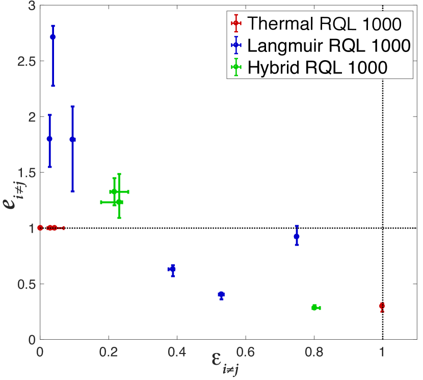
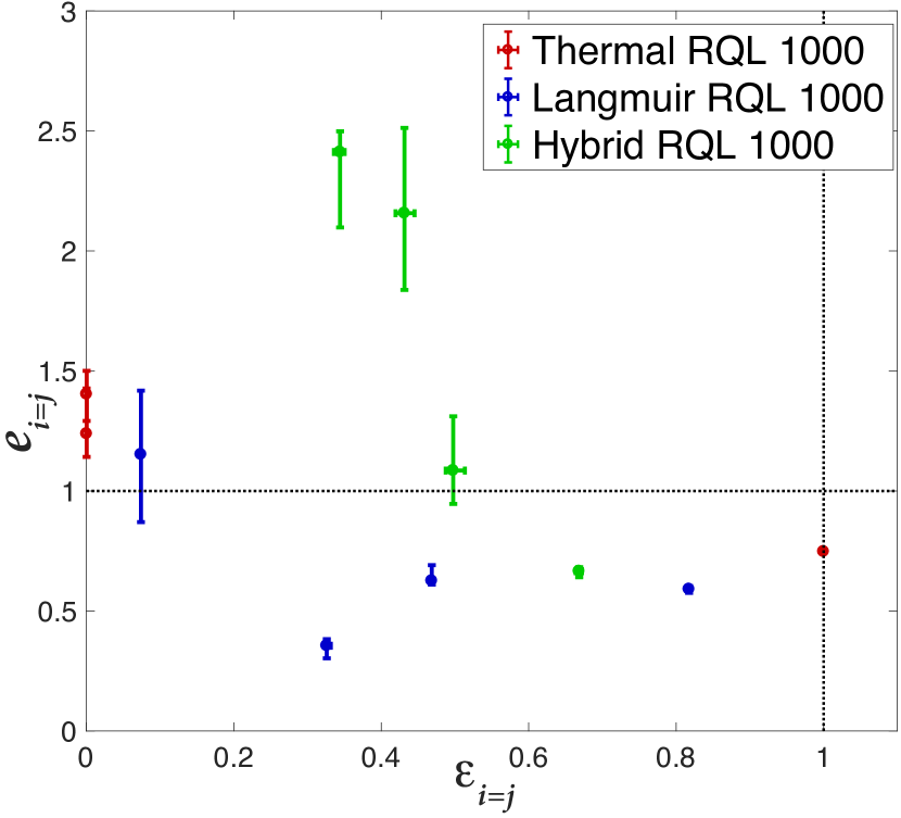
Figure 15: Comparison of second-order turbulent statistical profile representation errors (equation 41) with their variance-normalized amplitudes (equation 42) from the FNL solutions. This is done after temperatures have been scaled to have units of velocities using the available-potential energy technique described in section 3.2. The “Hybrid”- case is a mixture of the thermal-convection case and the Langmuir-turbulence case formulated so that the scaled turbulent temperature fluxes and turbulent velocity fluxes are similar in magnitude. When the turbulent energies (diagonal terms in the Reynolds-stress tensor, bottom) and transports (off-diagonal terms, top) are treated separately, variance-normalized amplitudes of these statistics are correlated with their representation error.

One takeaway from this work is that some turbulent-transport and energy profiles are well represented in the reduced models, while others are not. The ones that are well represented seem to be those which are most important for transporting energy from externally forced boundary conditions into the flow interior. It would be useful to be able to predict which of these transports would be most accurately represented without necessarily referring back to an ensemble of full-basis simulations. Monin-Obukhov similarity theory or (Kraus and Turner 1967) budgets might be revealing, but more simulations with both convective and stress forcing are needed to evaluate the robustness of this hypothesis.

As an idea for what might indicate the importance of second-order statistical transports, a 4-dimensional Reynolds-stress tensor was computed using the temperature scaling described in section 33.2 as well as the APE definition in equation 22 and normalized using the variances of all the elements at different depths and times:

$$\epsilon_{ij}=\frac{\sum_{z,t}\overline{q_{i}^{\prime}q_{j}^{\prime}\left(z,t\right)}^{2}}{\sum_{\left\{ij\right\}}\sum_{z,t}\overline{q_{i}^{\prime}q_{j}^{\prime}\left(z,t\right)}^{2}}$$ (42)

where $\left\{ij\right\}$ is the set of pairs of velocity-temperature components in consideration (energy and transport elements are treated separately for best results, so this will be either $i=j$ or $i\neq j$). This was then plotted against the representation error, $e_{ij}$ (see equation 41), for a variety of different cases. The results, shown in figure 15, indicate a weakly negative correlation between the error and the scaled Reynolds stress amplitude. Perhaps a more reasoned approach to determining the “importance” of these statistics might reveal a stronger correlation.

7 Conclusion

Two cases of developing ocean-surface boundary-layer turbulence were used to study the quasilinear reduced-model representation of flow statistics. In concrete terms, the reduced quasilinear model represented certain second-order turbulent transport and energy profiles in these cases qualitatively well (less than 30% error from the full-basis nonlinear profiles) using $\mathcal{O}\left(10^{-3}\right)$ retained POD modes. The profiles that were represented well appear to be correlated with their role driving the flow dynamics.

The case of surface-forced thermal convection in a deepening boundary layer exhibited nonuniform convergence of the statistical profiles towards complete representation, causing substantial inaccuracies in flow statistics. This was corrected for by restricting basis representation at large scales in a way that can be done dynamically at runtime. The reduced-basis quasilinear vertical statistics profiles in the Langmuir-turbulence case, of which there are many more than in the thermal-convection case that are non-trivial, exhibited intermediate convergence towards the full-basis nonlinear profiles before converging on the full-basis quasilinear profiles. Both of these properties were observed more thoroughly in an unrealistic miniature test case of the Langmuir turbulence.

What this means in broad terms is that a QL POD reduced model performs better than would be expected based naively on the isolated performances of the QL approximation and POD-based reduced-modeling: not only does QL allow for a smaller problem size and better runtime scalings than nonlinear POD reduced model; truncation of the QL approximation can add multi-scale structure missing from the full-basis QL solution, often producing flow features that resemble those of full-basis NL more so than full-basis QL. By better understanding these synergistic effects, it may be possible to craft QL POD reduced models into a cost-effective SGS model.

In addition to the performance of the cases studied, the potential for generalizing this framework can be acknowledged. Although only two examples of turbulence were tested of the many that must be modeled in an ESM, it should be noted that these were the only examples studied. Because there were no assumptions made that are specific to these cases in developing this QL POD reduced-model framework, it is reasonable to expect the framework to work similarly well with other types of boundary-layer turbulence in general, potentially addressing the drawbacks of the current approach of modeling different turbulent phenomena separately.

8 Acknowledgements

We thank Altan Allawala, Greg Chini, and Steve Tobias for helpful conversations. The authors are grateful to the Kavli Institute for Theoretical Physics for supporting the Program “Planetary Boundary Layers in Atmospheres, Oceans, and Ice on Earth and Moons” in Spring 2018 where some of this work was carried out. The research was supported in part by the National Science Foundation under Grant No. NSF PHY-1748958, NSF ONR N00014-17-1-2963, NSF OCE-1350795 as well as by the Institute at Brown for Environment and Society.

Appendix A Proper Orthogonal Decomposition in Homogeneous Dimensions

Begin with a field, $\psi\left(\mathbf{x}\right)$, defined over $n$ continuous and statistically homogeneous periodic dimensions that span $0$ to $L_{i}$ and define the volume $V={\displaystyle\prod_{i}^{n}L_{i}}$. For simplicity, inhomogeneous dimensions are not written explicitly but all variables can be a defined over any number of inhomogeneous dimensions without loss of generality. Because the statistics are homogeneous in $\mathbf{x}$, the covariance, $c_{2}$, indicating the second cumulant, must depend only on the field spacing:

$$c_{2}\left(\mathbf{x}_{1}-\mathbf{x}_{2}\right)=\overline{\psi(\mathbf{x}_{1})\psi(\mathbf{x}_{2})}$$ (43)

where the overline now specifically refers to a spatial average over the $n$ homogeneous dimensions. Introducing $\bar{\mathbf{x}}=\frac{1}{2}\left(\mathbf{x}_{1}+\mathbf{x}_{2}\right)$ and $\delta\mathbf{x}=\mathbf{x}_{1}-\mathbf{x}_{2}$, then this average can be written

$$c_{2}\left(\mathbf{x}_{1}-\mathbf{x}_{2}\right)=\frac{1}{V}\int_{\mathcal{V}_{\bar{x}}}d\bar{\mathbf{x}}\psi\left(\bar{\mathbf{x}}+\frac{\delta\mathbf{x}}{2}\right)\psi\left(\bar{\mathbf{x}}-\frac{\delta\mathbf{x}}{2}\right)$$ (44)

Where $\mathcal{V}_{\bar{x}}$ spans the entire domain in position space, $\left[0,L_{i}\right)$ for the $i$th homogeneous dimension. Then, writing the fields as a sum of their Fourier modes

$$\psi(\mathbf{x}_{1}) =\int_{\mathcal{V}_{k_{1}}}\frac{d\mathbf{k}_{1}}{\left(2\pi\right)^{n}}e^{i\mathbf{k}_{1}\cdot\mathbf{x}_{1}}\psi\left(\mathbf{k}_{1}\right)$$ (45)

$$\psi(\mathbf{x}_{2}) =\int_{\mathcal{V}_{k_{2}}}\frac{d\mathbf{k}_{2}}{\left(2\pi\right)^{n}}e^{i\mathbf{k}_{2}\cdot\mathbf{x}_{2}}\psi\left(\mathbf{k}_{2}\right)$$ (46)

where $\mathcal{V}_{k}$ spans the entire volume of wavenumber space, $\left(-\infty,+\infty\right)$ in each homogeneous dimension. Plugging this into the spatial average

$$c_{2}\left(\mathbf{x}_{1}-\mathbf{x}_{2}\right)=$$

$$\qquad\frac{1}{V}\int_{\mathcal{V}_{k_{1}},\mathcal{V}_{k_{2}}}\frac{d\mathbf{k}_{1}}{\left(2\pi\right)^{n}}\frac{d\mathbf{k}_{2}}{\left(2\pi\right)^{n}}\int_{\mathcal{V}_{\bar{x}}}d\bar{\mathbf{x}}$$

$$\qquad\qquad e^{i\mathbf{k}_{1}\cdot\left(\bar{\mathbf{x}}+\frac{\delta\mathbf{x}}{2}\right)}e^{i\mathbf{k}_{2}\cdot\left(\bar{\mathbf{x}}-\frac{\delta\mathbf{x}}{2}\right)}\psi(\mathbf{k}_{1})\psi(\mathbf{k}_{2})$$ (47)

$$c_{2}\left(\mathbf{x}_{1}-\mathbf{x}_{2}\right)=$$

$$\qquad\int_{\mathcal{V}_{k}}\frac{d\mathbf{k}_{1}d\mathbf{k}_{2}}{\left(2\pi\right)^{n}}\delta\left(\mathbf{k}_{1}+\mathbf{k}_{2}\right)$$

$$\qquad\qquad e^{i\mathbf{k}_{1}\cdot\frac{\delta\mathbf{x}}{2}}e^{-i\mathbf{k}_{2}\cdot\frac{\delta\mathbf{x}}{2}}\psi(\mathbf{k}_{1})\psi(\mathbf{k}_{2})$$ (48)

$$c_{2}\left(\mathbf{x}_{1}-\mathbf{x}_{2}\right)=$$

$$\qquad\int_{\mathcal{V}_{k}}\frac{d\mathbf{k}_{2}}{\left(2\pi\right)^{n}}e^{i\mathbf{k}_{1}\cdot\delta\mathbf{x}}\psi(\mathbf{k}_{1})\psi(\mathbf{k}_{1})^{*}$$ (49)

so the covariance matrix is diagonal in Fourier space, and therefore the POD modes are also Fourier modes in homogeneous dimensions.

References

- Adcroft et al. (2018) Adcroft, A., and Coauthors, 2018: Mitgcm user manual. MIT department of EAPS, URL http://mitgcm.org/download/manual/manual_20180114.pdf.
- Allawala and Marston (2016) Allawala, A., and J. B. Marston, 2016: Statistics of the stochastically-forced Lorenz attractor by the Fokker-Planck equation and cumulant expansions. Physical review. E, Statistical physics, plasmas, fluids, and related interdisciplinary topics, 94 (5), 052 218.
- Allawala et al. (2017) Allawala, A., S. M. Tobias, and J. B. Marston, 2017: Dimensional reduction of direct statistical simulation. arXiv preprint arXiv:1708.07805.
- Bachman et al. (2017) Bachman, S., B. Fox-Kemper, J. Taylor, and L. Thomas, 2017: Parameterization of frontal symmetric instabilities. i: Theory for resolved fronts. Ocean Modelling, 109, 72–95.
- Bartello and Holloway (1991) Bartello, P., and G. Holloway, 1991: Passive scalar transport in -plane turbulence. Journal of Fluid Mechanics, 223, 521–536, 10.1017/S0022112091001532, URL http://journals.cambridge.org/article_S0022112091001532.
- Batchelor (1952) Batchelor, G., 1952: Diffusion in a field of homogeneous turbulence: Ii. the relative motion of particles. Mathematical Proceedings of the Cambridge Philosophical Society, Cambridge University Press, Vol. 48, 345–362.
- Bauer et al. (2015) Bauer, P., A. Thorpe, and G. Brunet, 2015: The quiet revolution of numerical weather prediction. Nature, 525 (7567), 47–55, 10.1038/nature14956, URL http://dx.doi.org/10.1038/nature14956.
- Belcher et al. (2012) Belcher, S. E., and Coauthors, 2012: A global perspective on langmuir turbulence in the ocean surface boundary layer. Geophysical Research Letters, 39 (18).
- Bony et al. (2015) Bony, S., and Coauthors, 2015: Clouds, circulation and climate sensitivity. Nature Geoscience, 8 (4), 261–268.
- Bouchet et al. (2013) Bouchet, F., C. Nardini, and T. Tangarife, 2013: Kinetic Theory of Jet Dynamics in the Stochastic Barotropic and 2D Navier-Stokes Equations. Journal of Statistical Physics, 153 (4), 572–625, 10.1007/s10955-013-0828-3, URL http://dx.doi.org/10.1007/s10955-013-0828-3.
- Canuto and Minotti (2001) Canuto, V. M., and F. Minotti, 2001: Mixing and transport in stars - I. Formalism: momentum, heat and mean molecular weight. Mon. Not. Roy. Ast. Soc., 328, 829–838.
- Chaalal et al. (2016) Chaalal, F. A., T. Schneider, B. Meyer, and B. Marston, 2016: Cumulant expansions for atmospheric flows. New Journal of Physics, 18 (2), 1–24.
- Craik (1977) Craik, A. D. D., 1977: The generation of langmuir circulations by an instability mechanism. Journal of Fluid Mechanics, 81 (2), 209–223.
- Doney et al. (2004) Doney, S. C., and Coauthors, 2004: Evaluating global ocean carbon models: The importance of realistic physics. Global Biogeochem. Cycles, 18 (3), n/a–n/a, 10.1029/2003gb002150, URL http://dx.doi.org/10.1029/2003gb002150.
- Farrell and Ioannou (2007) Farrell, B. F., and P. J. Ioannou, 2007: Structure and spacing of jets in barotropic turbulence. Journal of the Atmospheric Sciences, 64 (10), 3652–3665.
- Foken (2006) Foken, T., 2006: 50 years of the monin–obukhov similarity theory. Boundary-Layer Meteorology, 119 (3), 431–447.
- Fox-Kemper et al. (2014) Fox-Kemper, B., S. D. Backman, B. Pearson, and S. Reckinger, 2014: Principles and advances in subgrid modelling for eddy-rich simulations. Clivar Exchanges, 19 (2), 42–46.
- Fox-Kemper and Ferrari (2008) Fox-Kemper, B., and R. Ferrari, 2008: Parameterization of mixed layer eddies. part i: Theory and diagnosis. Journal of Physical Oceanography, 38 (6), 1145–1165.
- Hamlington et al. (2014) Hamlington, P. E., L. P. V. Roekel, B. Fox-Kemper, K. Julien, and G. P. Chini, 2014: Langmuir–Submesoscale Interactions: Descriptive Analysis of Multiscale Frontal Spindown Simulations. J. Phys. Oceanogr., 44 (9), 2249–2272, 10.1175/jpo-d-13-0139.1, URL http://dx.doi.org/10.1175/JPO-D-13-0139.1.
- Harcourt (2013) Harcourt, R. R., 2013: A second-moment closure model of langmuir turbulence. Journal of Physical Oceanography, 43 (4), 673–697.
- Herring (1963) Herring, J. R., 1963: Investigation of problems in thermal convection. Journal of Atmospheric Sciences, 20, 325–338.
- Holmes et al. (2012) Holmes, P., J. L. Lumley, G. Berkooz, and C. W. Rowley, 2012: Turbulence, Coherent Structures, Dynamical Systems and Symmetry. 2nd ed., Cambridge University Press, Cambridge.
- Kang et al. (2009) Kang, S. M., D. M. Frierson, and I. M. Held, 2009: The tropical response to extratropical thermal forcing in an idealized gcm: The importance of radiative feedbacks and convective parameterization. Journal of the atmospheric sciences, 66 (9), 2812–2827.
- Kolmogorov (1941) Kolmogorov, A. N., 1941: Dissipation of energy in locally isotropic turbulence. Dokl. Akad. Nauk SSSR, Vol. 32, 16–18.
- Kraus and Turner (1967) Kraus, E., and J. Turner, 1967: A one-dimensional model of the seasonal thermocline. II: The general theory and its consequences. Tellus, 19, 98–106.
- Krause and Raedler (1980) Krause, F., and K. H. Raedler, 1980: Mean-field magnetohydrodynamics and dynamo theory. Pergamon Press.
- Large et al. (1997) Large, W. G., G. Danabasoglu, S. C. Doney, and J. C. McWilliams, 1997: Sensitivity to Surface Forcing and Boundary Layer Mixing in a Global Ocean Model: Annual-Mean Climatology. J. Phys. Oceanogr., 27 (11), 2418–2447, 10.1175/1520-0485(1997)027<2418:stsfab>2.0.co;2, URL http://dx.doi.org/10.1175/1520-0485(1997)027<2418:stsfab>2.0.co;2.
- Large et al. (1994) Large, W. G., J. C. McWilliams, and S. C. Doney, 1994: Oceanic vertical mixing: A review and a model with a nonlocal boundary layer parameterization. Reviews of Geophysics, 32 (4), 363 – 403.
- Leibovich (1983) Leibovich, S., 1983: The form and Dynamics of Langmuir Circulations. Annu. Rev. Fluid Mech., 15 (1), 391–427, 10.1146/annurev.fl.15.010183.002135, URL http://dx.doi.org/10.1146/annurev.fl.15.010183.002135.
- Li et al. (2019) Li, Q., and Coauthors, 2019: Comparing ocean boundary vertical mixing schemes including Langmuir turbulence. Journal of Advances in Modeling Earth Systems (JAMES).
- Malkus (1954) Malkus, W., 1954: The Heat Transport and Spectrum of Thermal Turbulence. Proceedings of the Royal Society of London. Series A, Mathematical and Physical Sciences, 225 (1161), 196–212.
- Maltrud and Vallis (1991) Maltrud, M. E., and G. K. Vallis, 1991: Energy spectra and coherent structures in forced two-dimensional and beta-plane turbulence. Journal of Fluid Mechanics, 228, 321–342.
- Marston et al. (2016) Marston, J., G. Chini, and S. Tobias, 2016: Generalized quasilinear approximation: Application to zonal jets. Physical Review Letters, 116 (21), 214 501.
- Marston (2010) Marston, J. B., 2010: Statistics of the general circulation from cumulant expansions. Chaos, 20 (4), 041 107.
- Marston et al. (2008) Marston, J. B., E. Conover, and T. Schneider, 2008: Statistics of an Unstable Barotropic Jet from a Cumulant Expansion. Journal of Atmospheric Sciences, 65, 1955, 10.1175/2007JAS2510.1, 0705.0011.
- Marston et al. (2019) Marston, J. B., W. Qi, and S. M. Tobias, 2019: Direct Statistical Simulation of a Jet in Zonal Jets: Phenomenology, Genesis, and Physics (arXiv:1412.0381). Cambridge University Press.
- McWilliams and Sullivan (2000) McWilliams, J. C., and P. P. Sullivan, 2000: Vertical Mixing by Langmuir Circulations. Spill Science & Technology Bulletin, 6 (3-4), 225–237, 10.1016/s1353-2561(01)00041-x, URL http://dx.doi.org/10.1016/s1353-2561(01)00041-x.
- McWilliams et al. (1997) McWilliams, J. C., P. P. Sullivan, and C. Moeng, 1997: Langmuir turbulence in the ocean. Journal of Fluid Mechanics, 334, 1–30.
- Mellor and Yamada (1974) Mellor, G. L., and T. Yamada, 1974: A hierarchy of turbulence closure models for planetary boundary layers. Journal of the Atmospheric Sciences, 31, 1791–1806.
- O’Gorman and Schneider (2007) O’Gorman, P. A., and T. Schneider, 2007: Recovery of atmospheric flow statistics in a general circulation model. Geophysical Research Letters, 34, 524 – 535.
- Pausch et al. (2019) Pausch, M., Q. Yang, Y. Hwang, and B. Eckhardt, 2019: Quasilinear approximation for exact coherent states in parallel shear flows. Fluid Dynamics Research, 51, 1–15.
- Rüdiger (1989) Rüdiger, G., 1989: Differential rotation and stellar convection: Sun and solar-type stars, Vol. 5. Gordon & Breach, New York.
- Salmon (1998) Salmon, R., 1998: Lectures on Geophysical Fluid Dynamics. Oxford University Press, New York.
- Schmidt and Schumann (1989) Schmidt, H., and U. Schumann, 1989: Coherent structure of the convective boundary layer derived from large-eddy simulation. Journal of Fluid Mechanics, 200, 511–562.
- Sirovich (1989) Sirovich, L., 1989: Chaotic dynamics of coherent structures. Physica D: Nonlinear Phenomena, 37 (1-3), 126–145.
- Skitka (2019) Skitka, J., 2019: Quasilinear modeling of planetary boundary-layer turbulence [PhD Thesis]. Providence, RI: Brown University.
- Spiegel (1962) Spiegel, E. A., 1962: Thermal Turbulence at Very Small Prandtl Number. Journal of Geophysical Research, 67 (8), 3063–&.
- Squire and Bhattacharjee (2015) Squire, J., and A. Bhattacharjee, 2015: Statistical Simulation of the Magnetorotational Dynamo. Physical Review Letters, 114 (8), 085 002–5.
- Srinivasan and Young (2012a) Srinivasan, K., and W. Young, 2012a: Zonostrophic instability. Journal of the atmospheric sciences, 69 (5), 1633–1656.
- Srinivasan and Young (2012b) Srinivasan, K., and W. R. Young, 2012b: Zonostrophic instability. J. Atmos. Sci., 69, 1633–1656.
- Stephens (2005) Stephens, G. L., 2005: Cloud Feedbacks in the Climate System: A Critical Review. Journal of Climate, 18 (2), 237–273.
- Stocker et al. (2013) Stocker, T. F., and Coauthors, 2013: Climate change 2013: The physical science basis. Tech. rep. 1535 pp.
- Sullivan et al. (1994) Sullivan, P. P., J. C. McWilliams, and C.-H. Moeng, 1994: A subgrid-scale model for large-eddy simulation of planetary boundary-layer flows. Boundary-Layer Meteorology, 71 (3), 247–276.
- Thomas et al. (2015) Thomas, V. L., B. F. Farrell, P. J. Ioannou, and D. F. Gayme, 2015: A minimal model of self-sustaining turbulence. Physics of Fluids, 27 (10), 105 104, 10.1063/1.4931776.
- Thorpe (2004) Thorpe, S., 2004: Langmuir Circulation. Annual Review of Fluid Mechanics, 36 (1), 55–79, 10.1146/annurev.fluid.36.052203.071431, URL http://dx.doi.org/10.1146/annurev.fluid.36.052203.071431.
- Tobias et al. (2011) Tobias, S. M., K. Dagon, and J. B. Marston, 2011: Astrophysical fluid dynamics via direct statistical simulation. The Astrophysical Journal, 727, 127.
- Tobias and Marston (2013) Tobias, S. M., and J. B. Marston, 2013: Direct Statistical Simulation of Out-of-Equilibrium Jets. Physical Review Letters, 110 (10), 104 502.
- Van Roekel et al. (2012) Van Roekel, L., B. Fox-Kemper, P. Sullivan, P. Hamlington, and S. Haney, 2012: The form and orientation of langmuir cells for misaligned winds and waves. Journal of Geophysical Research: Oceans, 117 (C5).
- Vedenov et al. (1961) Vedenov, A. A., E. P. Velikhov, and R. Z. Sagdeev, 1961: Quasilinear theory of plasma oscillations. Proceedings of IAEA Conference on Plasma Physics and Controlled Nuclear Fusion Research, 465–475.
- Wang et al. (2012) Wang, Z., I. Akhtar, J. Borggaard, and T. Iliescu, 2012: Proper orthogonal decomposition closure models for turbulent flows: a numerical comparison. Computer Methods in Applied Mechanics and Engineering, 237, 10–26.