Gradient projection and conditional gradient methods for constrained nonconvex minimization

Abstract.

Minimization of a smooth function on a sphere or, more generally, on a smooth manifold, is the simplest non-convex optimization problem. It has a lot of applications. Our goal is to propose a version of the gradient projection algorithm for its solution and to obtain results that guarantee convergence of the algorithm under some minimal natural assumptions. We use the Ležanski-Polyak-Lojasiewicz condition on a manifold to prove the global linear convergence of the algorithm. Another method well fitted for the problem is the conditional gradient (Frank-Wolfe) algorithm. We examine some conditions which guarantee global convergence of full-step version of the method with linear rate.

1. Introduction

Consider minimization of a smooth function $f(x)$ on a closed set $Q$ in the Euclidean space $(\mathbb{R}^{n},\|\cdot\|)$

(1) $$\min_{x\in Q}f(x).$$

Traditionally the set $Q$ and the function $f$ are assumed to be convex; in such convex setting the problem is well studied and numerous algorithms are known, see e.g. [7, 8, 29, 30] for details. We plan to address the situation when the function or/and the set are nonconvex.

The function $f$ under consideration is smooth with the Lipschitz continuous gradient, but nonconvex. Regarding the set $Q$, we mostly suppose that it is proximally smooth [36, 10, 9]. In particular we consider the next important cases:
1) $Q=S_{R}=\{x\in\mathbb{R}^{n}\ |\ ||x||=R\}$ (minimization on the sphere),
2) $Q=\{x\in\mathbb{R}^{n}\ |\ g(x)=0\}$, $g:\mathbb{R}^{n}\to\mathbb{R}^{m}$ (equality type constraints),
3) $Q$ is the boundary of a strongly convex set $B\subset\mathbb{R}^{n}$.

Minimization on the sphere has numerous applications, for instance finding minimal eigenvalue of a symmetric matrix $A\in\mathbb{R}^{n\times n}$ (then $f(x)=(Ax,x)$, $Q=S_{1}$) or choosing step-size in trust-region methods [11]. The set $Q$ is obviously nonconvex thus (1) is an example of nonconvex optimization problems. The pioneering work in the field is [25]. Special case of problem (1) (for quadratic $f(x)$) has been studied by Hager [16]; the solution can be reduced to solving 1D equations. Later publications include [1, 28, 26, 35, 37], in most of them $Q$ is a smooth (Riemannian) manifold. But in general, research in nonconvex optimization is much less intensive than in convex case. The main approaches use generalized convexity on the set and/or consider geodesic-related steps. In contrast, we use neither of these. There are numerous methods for optimization with equality type constrains, see e.g [31, Chapter 7], [7]. However, most of them generate points which are not admissible ($x_{k}\notin Q$) while our purpose is to develop methods with admissible iterations.

The contribution of the present paper is triple:

1. We propose a new approach to the gradient projection algorithm for constrained optimization, based on the idea of upper approximation of the objective function. The resulting method is the gradient projection algorithm with constant step-size; it differs from versions proposed in [25]. Moreover we prove its convergence to a stationary point without any convexity-like assumptions.

2. We generalize well known in unconstrained optimization the Polyak-Lojasiewicz condition on the class of problems (1). Under this assumption we prove linear convergence of the gradient projection algorithm (with projection on the tangent subspace and a variant combined with the Newton method) to a global extremum under assumption of proximal smoothness of the manifold $Q$. As an example we consider a quadratic form on the unit sphere.

3. For approximately linear objective functions we propose a new version of the Frank-Wolfe (conditional gradient) method and establish its linear convergence to a global minimum in problem (1). We prove linear convergence of the method for a surface, which is the boundary of a strongly convex set. Note, that such surface is not necessary smooth.

In the paper [4] linear convergence of the gradient projection algorithm was proved for a proximally smooth set with constant $R$ and for a strongly convex function with constant of strong convexity $\varkappa$ and Lipschitz constant $L$ under assumption $\frac{L}{\varkappa}<R$. The last inequality is essential for linear convergence of the method. In subsection 3.1 we prove convergence of the standard gradient projection algorithm to a stationary point of the problem (1) for any function with the Lipschitz continuous gradient and for any proximally smooth set.

In subsection 3.2 we extend the Polyak-Lojasiewicz condition (well known in unconstrained minimization) [27, 33, 19] for the constrained case (1) with differentiable function and $C^{1}$ smooth manifold $Q$. We want to pay attention that this generalization is in fact some variant of the error bound condition for the case of smooth set $Q$.

On the base of the new definition from subsection 3.2 we prove in subsection 3.3 convergence of the gradient projection algorithm for $Q=S_{1}$. For the case of general $C^{1}$ smooth and proximally smooth manifold of codimension 1 we prove it in subsection 3.4. In contrast with other approaches our algorithms represent variants of the gradient projection algorithm with admissible points $x_{k}\in Q$ and linear rate of convergence.

In subsection 3.5 we consider the situation when the gradient projection algorithm can be finalized by use of the Newton method. This is standard practice, except that we are dealing with nonconvex problem.

Concluding section 3, we prove the Ležanski-Polyak-Lojasiewicz condition for the quadratic function on the sphere. Thus we extend the result [17] by clarifying constant $\mu$ in this condition. It is essential for estimate of the error for the gradient projection algorithm in the case $Q=S_{1}$.

In section 4 we consider application of the Frank-Wolfe method for solving the problem (1) in the case when $Q$ is the boundary of a strongly convex set of radius $R$. It is well known that if the set $Q$ is a convex compact and $f$ is a Lipschitz differentiable convex function then the method converges (with respect to the objective function) with sublinear rate. In [14] the authors discuss the choice of step-size in the method. In [26] the author proved that under certain assumptions in the case of convex compact set $Q$ and for a (nonconvex) function with the Lipschitz continuous gradient the Frank-Wolfe method converges to a stationary point in the problem (1) with sublinear rate.

We prove linear rate of convergence with respect to the point. In subsection 4.1 we proved it for so-called linear approximative function and in subsection 4.2 we proved it for a function with gradient domination. In fact in both subsections the general idea consists in the fact that radius of ”curvature” of the level sets for our function is larger than the radius of strong convexity. This leads to the results. We only want to point out that we take the notation of radius of ”curvature” in the sense of supporting principles for proximally smooth and strongly convex sets.

For completeness in Appendix we prove necessary condition of minimum in the problem (1) for a proximally smooth set $Q$ and a function with the Lipschitz continuous gradient.

All mentioned parts are gathered together by the possibility of certain “spherical” approximation (via the supporting principles) for the set/surface $Q$ in problem (1).

The most part of mentioned results takes place in the case of the real Hilbert space. Sometimes obvious patches should be applied in the infinite dimension case, for example compactness of the set $Q$ in Theorem 1.

2. Definitions and main notations

Let $B_{R}(a)=\{x\in\mathbb{R}^{n}\ |\ \|x-a\|\leq R\}$ be the ball with center $a\in\mathbb{R}^{n}$ and radius $R>0$. For a set $Q\subset\mathbb{R}^{n}$ the sets $\mbox{\rm cl}\,Q$, $\mbox{\rm int}\,Q$, $\partial Q$ are the closure, the interior and the boundary of $Q$, respectively. We also denote by $\partial Q$ the edge of the surface $Q$.

Let $P_{Q}$ be the operator of metric projection on the set $Q$, i.e. $P_{Q}(x)=\{y\in Q:||y-x||=\inf_{z\in Q}||x-z||\}$. In general, $P_{Q}$ can be set-valued for nonconvex sets, but for proximally smooth sets (see below) it is single-valued (provided $x$ is close enough to $Q$).

For a closed set $Q\subset\mathbb{R}^{n}$ the normal cone of proximal normals (or simply the normal cone) at a point $x\in Q$ is defined as follows [9]

$$N(Q,x)=\{p\in\mathbb{R}^{n}\ |\ \exists\delta>0\ P_{Q}(x+\delta p)=x\}.$$

If the set $Q$ is convex, then $N(Q,x)$ coincides with normal cone in the sense of convex analysis.

A closed set $Q\subset\mathbb{R}^{n}$ is called proximally smooth with constant $R>0$ [36, 10, 9] if the distance function $\varrho(x,Q)=\varrho_{Q}(x)=\inf\limits_{a\in Q}\|x-a\|$ is continuously Frechet differentiable on the set $U_{Q}(R)=\{x\in\mathbb{R}^{n}\ |\ 0<\varrho_{Q}(x)<R\}$. The equivalent properties for a proximally smooth set with constant $R$ are

1) $P_{Q}:U_{Q}(R)\to Q$ is a single-valued continuous function,

2) supporting principle: $p\!\in\!N(Q,x)$, $\|p\|\!=\!1$, if and only if $Q\cap\mbox{\rm int}\,B_{R}(x+Rp)=\emptyset$.

Note that the mapping $Q\ni x\to N(Q,x)$ is upper semicontinuous for a proximally smooth set $Q$ with constant $R$. For a point $x\in\mbox{\rm int}\,Q$ we have $N(Q,x)=0$ and it is sufficient to prove upper semicontinuity on the boundary $\partial Q$. Choose $x_{k}\in\partial Q$, $x_{k}\to x\in\partial Q$, and $p_{k}\in N(Q,x_{k})$, $\|p_{k}\|=1$, with $p_{k}\to p$. Suppose that $p\notin N(Q,x)$, the last means that $N(Q,\cdot)$ is not upper semicontinuous at the point $x$. By the supporting principle for proximally smooth sets

$$\exists\,\overline{x}\in Q\cap\mbox{\rm int}\,B_{R}(x+Rp).$$

The sets $\mbox{\rm int}\,B_{R}(x_{k}+Rp_{k})$ converge to the set $\mbox{\rm int}\,B_{R}(x+Rp)$ in the Hausdorff metric, thus $\overline{x}\in Q\cap\mbox{\rm int}\,B_{R}(x_{k}+Rp_{k})$ for sufficiently large $k$. A contradiction.

If we consider a continuously differentiable $(n-1)$-dimensional surface $Q$ without edge which is also proximally smooth with constant $R>0$, then for any point $x\in Q$ the normal cone $N(Q,x)$ is 1-dimensional subspace. If $\|p\|=1$ and $p\in N(Q,x)$ then the surface $Q$ is trapped between the supporting spheres (see supporting principle 2)):

(2) $$Q\subset\left(\mathbb{R}^{n}\backslash\mbox{\rm int}\,B_{R}(x-Rp)\right)\cap\left(\mathbb{R}^{n}\backslash\mbox{\rm int}\,B_{R}(x+Rp)\right).$$

A closed convex set $B\subset\mathbb{R}^{n}$ is called strongly convex of radius $r>0$ if it can be represented in the form $B=\bigcap\limits_{x\in X}B_{r}(x)$ [36, 5]. There are few equivalent properties for strong convexity:
1) A convex compact set $B\subset\mathbb{R}^{n}$ is strongly convex of radius $r$ if and only if for any pair of points $x,y\in B$ the ball with center $\frac{1}{2}(x+y)$ of radius $\frac{1}{8r}\|x-y\|^{2}$ belongs to $B$ [22, 34, 2].
2) Another equivalent property for strong convexity is supporting principle: for any $x\in\partial B$ and $p\in N(B,x)$, $\|p\|=1$, we have

$$B\subset B_{r}(x-rp).$$

3) The set $B\subset\mathbb{R}^{n}$ is strongly convex of radius $r$ if and only if for any unit vectors $p,q$ and for supporting elements $x_{p}=\arg\max\limits_{x\in B}(p,x)$, $x_{q}=\arg\max\limits_{x\in B}(q,x)$ we have the next inequality [36, Proposition 2.8]

$$\|x_{p}-x_{q}\|\leq r\|p-q\|.$$

If $Q$ is a smooth manifold, then the subspace $T_{x}$ is the tangent subspace to $Q$ at a point $x\in Q$, i.e.

$$T_{x}=\{v\in\mathbb{R}^{n}:\varrho(x+tv,Q)=o_{v}(t)\},$$

where $\lim\limits_{t\to+0}\frac{o_{v}(t)}{t}=0$ for all $v\in T_{x}$.

Define $\mathcal{L}_{f}(\beta)=\{x\in\mathbb{R}^{n}\ |\ f(x)\leq\beta\}$ the lower level set of the function $f$.

We say that the function $f$ has the Lipschitz continuous gradient with constant $L_{1}>0$ if

(3) $$\|f^{\prime}(x)-f^{\prime}(y)\|\leq L_{1}\|x-y\|,\quad\forall x,y.$$

It is well known that (3) implies the upper bound for $f$ [29, Lemma 1.2.3]:

(4) $$\left|f(y)-f(x)-(f^{\prime}(x),y-x)\right|\leq\frac{C}{2}||y-x||^{2},\quad\forall x,y,$$

for any $C\geq L_{1}$.

We write $f(t)\asymp g(t),t\in\mathbb{R}^{1}$, $t\to+0$, if there exist $0<C_{1}<C_{2}$ and $\delta>0$ such that $C_{1}f(t)\leq g(t)\leq C_{2}f(t)$ for all $t\in(0,\delta)$.

For a differentiable vector function $g(x)=(g_{1}(x),\dots,g_{m}(x))^{T}$ denote the Jacobi matrix as

$$g^{\prime}(x)=(g_{1}^{\prime}(x)\dots g_{m}^{\prime}(x))$$

and we treat $g_{i}^{\prime}(x)$ as columns.

The set $\Omega\subset Q$ is the set of stationary points of the differentiable function $f$ on the set $Q$ (which is associated with the problem (1)) if for any point $x\in\Omega$ we have $f^{\prime}(x)\in-N(Q,x)$. The last inclusion is necessary condition of optimality for a proximally smooth set $Q$ and a smooth function $f$. We prove it in Appendix for completeness.

3. The gradient projection algorithm

The gradient projection algorithm for (1) in convex case has been proposed in [18, 22]. The simplest version (with constant step-size) looks as follows: for an iteration $x_{k}\in Q$ it generates the new point $x_{k+1}$ as the minimizer of the upper bound on $Q$ (with $C_{1}\geq L_{1}$) or, equivalently, as projection of the gradient step on $Q$:

Gradient Projection Algorithm (GPA1)

Step 1. Choose a constant $C_{1}>0$, initial point $x_{0}\in Q$ and put $k=0$.

Step 2. Repeat

(5) $$\begin{array}[]{rl}x_{k+1}\!\!\!\!&=\displaystyle\arg\min_{x\in Q}\left\{f(x_{k})+(f^{\prime}(x_{k}),x-x_{k})+\frac{C_{1}}{2}||x-x_{k}||^{2}\right\}=\\[8.53581pt] &=\displaystyle P_{Q}\left(x_{k}-\frac{1}{C_{1}}f^{\prime}(x_{k})\right),\end{array}$$

The condition $C_{1}\geq L_{1}$ is equivalent to choice of the constant step-size $t\leq\frac{1}{L_{1}}$. Below we shall consider the extensions of the method for nonconvex set $Q$ and nonconvex function $f(x)$.

One of the possible ways for extension is gradient projection along geodesics proposed by Luenberger [25]. It is not hard to design geodesics on the sphere (arcs of big circles on the sphere), but the original algorithm in [25] requires one-dimensional minimization on each iteration. Another problem is that in the case of an arbitrary manifold $Q$ construction of geodesics is a hard procedure. Thus we avoid geodesics and try to deal with gradient projection method with constant step-size in the form (5).

3.1. The case of an arbitrary proximally smooth set $Q$. General algorithm

The next result shows that for any function $f:\mathbb{R}^{n}\to\mathbb{R}$ with the Lipschitz continuous gradient and for any proximally smooth set $Q\subset\mathbb{R}^{n}$ iterations of the standard gradient projection algorithm (5) are well-defined and converge to a stationary point of the function $f$ on the set $Q$ for the appropriate choice of the step-size.

Theorem 1.

Let $Q\subset\mathbb{R}^{n}$ be a bounded proximally smooth set with constant $R>0$. Suppose that the function $f:\mathbb{R}^{n}\to\mathbb{R}$ is the Lipschitz continuous with constant $L>0$ and its gradient $f^{\prime}$ is also the Lipschitz continuous with constant $L_{1}>0$. Take $C>0$ with $\frac{L}{C+L_{1}}<R$. Then for any $x_{0}\in Q$ GPA1 with $C_{1}=C+L_{1}$ converges to the set of stationary points $\Omega$: $\lim\limits_{k\to\infty}\varrho_{\Omega}(x_{k})=0$ and

$$f(x_{k+1})+\frac{C}{2}\|x_{k+1}-x_{k}\|^{2}\leq f(x_{k})$$

for all $k\geq 0$.

Proof. Define for each natural $k$ the function

$$\psi_{k}(x)=f(x_{k})+(f^{\prime}(x_{k}),x-x_{k})+\frac{C+L_{1}}{2}\|x-x_{k}\|^{2}.$$

It’s easy to see (due to the Lipschitz continuity of gradient $f^{\prime}$) that

$$\psi_{k}(x)\geq f(x)+\frac{C}{2}\|x-x_{k}\|^{2}$$

for all $x\in\mathbb{R}^{n}$ and

$$\varrho_{Q}\left(x_{k}-\frac{1}{C+L_{1}}f^{\prime}(x_{k})\right)\leq\left\|\frac{1}{C+L_{1}}f^{\prime}(x_{k})\right\|\leq\frac{L}{C+L_{1}}<R.$$

Hence the distance from the point $x_{k}-\frac{1}{C+L_{1}}f^{\prime}(x_{k})$ to the set $Q$ is less than $R$ and the metric projection $x_{k+1}$ is defined uniquely by the definition of proximally smooth set. We have

$$f(x_{k})=\psi_{k}(x_{k})\geq\psi_{k}(x_{k+1})\geq f(x_{k+1})+\frac{C}{2}\|x_{k+1}-x_{k}\|^{2}.$$

Assume that $\lim_{k\to\infty}\varrho_{\Omega}(x_{k})\neq 0$ for some sequence $\{x_{k}\}\subset Q$ which is generated by the gradient projection algorithm. Then there is a number $\varepsilon>0$ and a subsequence $\{x_{k_{m}}\}\subset\{x_{k}\}$ with $\varrho_{\Omega}(x_{k_{m}})\geq\varepsilon$ for all $m$. Consider a converging subsequence of the sequence $\{x_{k_{m}}\}$ (that again is denoted by $\{x_{k_{m}}\}$) and $x_{*}=\lim\limits_{m\to\infty}x_{k_{m}}$. Then from the necessary conditions of minimum of the function $\psi_{k_{m}}$ on the set $Q$ we get

$$\psi^{\prime}_{k}(x_{k_{m}+1})\in-N(Q,x_{k_{m}+1}),$$

in other words

$$f^{\prime}(x_{k_{m}})+(C+L_{1})(x_{k_{m}+1}-x_{k_{m}})\in-N(Q,x_{k_{m}+1}).$$

Passing to the limit as $m\to\infty$, using upper semicontinuity of the normal cone $N(Q,\cdot)$ and the property $\lim_{m\to\infty}(x_{k_{m}+1}-x_{k_{m}})=0$ we have

$$f^{\prime}(x_{*})\in-N(Q,x_{*}).$$

Thus $\lim\limits_{m\to\infty}\varrho_{\Omega}(x_{k_{m}})=0$, a contradiction. ∎

With the help of Theorem 1 we can find a stationary point with error $\varepsilon>0$, namely we can find a point $x\in Q$ with $\varrho(0,-f^{\prime}(x)-N(Q,x))<\varepsilon$.

Stationary-point Algorithm

Step 1. Choose $\varepsilon>0$ and $C>\max\{0,\frac{L}{R}-L_{1}\}$. Put $\Delta f=\sup_{Q}f-\inf_{Q}f$, $\delta=\frac{\varepsilon}{C+2L_{1}}$, and set $k=0$.

Step 2. Perform a Step 2 (5) of GPA1 with $C_{1}=C+L_{1}$.

Step 3. If $\|x_{k}-x_{k+1}\|\geq\delta$, increase $k$ and continue to the Step 2.

Otherwise stop the algorithm and return $x_{k+1}$ as the solution.

The algorithm do at most $N=\big{\lfloor}\frac{2\Delta f}{C\delta^{2}}\big{\rfloor}+1$ steps. Assume the contrary, that $\|x_{k+1}-x_{k}\|\geq\delta$ for $k=0,\dots,N-1$. Then assumptions of Theorem 1 holds, thus $\frac{C}{2}\delta^{2}\leq f(x_{k})-f(x_{k+1})$ and after $N$ steps we get

$$f(x_{0})-f(x_{N})\geq N\frac{C}{2}\delta^{2}>\Delta f,$$

i.e. a contradiction. When the algorithm stops with $\|x_{k}-x_{k+1}\|<\delta$, by the optimality condition for the function $\psi_{k}$ we get

$$f^{\prime}(x_{k})+(C+L_{1})(x_{k+1}-x_{k})\in-N(Q,x_{k+1}).$$

Using the Lipschitz continuity of $f^{\prime}$ we obtain

$$\varrho(f^{\prime}(x_{k+1}),-N(Q,x_{k+1}))\leq\delta(C+2L_{1})=\varepsilon.$$

Note that the parameter $C$ of the step $t=\frac{1}{C+L_{1}}$ depends on Lipschitz constant $L$ of the function $f$ because the point $x_{k}-tf^{\prime}(x_{k})$ should not go very far from the set $Q$. Moreover, conditions on constant $C$ mean that the step-size $t$ satisfies the inequality $t<\min\left\{\frac{R}{L},\frac{1}{L_{1}}\right\}$.

Example 1.

Sometimes projection can be found explicitly, for example for the unit sphere $Q=S_{1}$:

(6) $$x_{k+1}=\frac{x_{k}-tf^{\prime}(x_{k})}{\|x_{k}-tf^{\prime}(x_{k})\|},$$

thus the algorithm is the gradient-projection method with constant step-size.

By Proposition 1 the first-order optimality condition in (1) for $Q=S_{1}$ means $f^{\prime}(x)=\lambda x,\,\|x\|=1,\lambda\in\mathbb{R}$, and it can be immediately rewritten in the form

(7) $$\|(I-xx^{T})f^{\prime}(x)\|=0,$$

(here $I$ is the unit matrix) or as

(8) $$\|L_{1}x-f^{\prime}(x)\|=|(L_{1}x-f^{\prime}(x),x)|.$$

3.2. The Ležanski-Polyak-Lojasiewicz condition on a manifold.

Now the main task is to propose conditions which guarantee convergence of the method to the global minimum in the problem (1) and to estimate the rate of convergence.

In unconstrained minimization we have such powerful tool as convexity; gradient method for convex functions converges to global minima while for strongly convex functions one has linear rate of convergence. There are extensions of convexity for minimization on manifolds, see e.g. the monograph [35] and the paper [28]. Unfortunately there exist no (globally) convex functions on compact manifolds [28], thus we need some other tools.

However in the unconstrained case there are conditions which validate convergence for nonconvex functions. Probably the first one is due to T. Ležanski [23, 24]. He considered a problem of unconstrained minimization for a Lipschitz differentiable function $f$ such that there exists a positive continuous function $\varphi$ with

$$\|f^{\prime}(x)\|\geq\varphi(f(x)-f_{0}),\quad\forall x\in\mathbb{R}^{n},\qquad f_{0}=\min\limits_{x\in\mathbb{R}^{n}}f(x),\quad\int\limits_{0}^{f(x)-f_{0}}\frac{ds}{\varphi(s)}<\infty.$$

Under these assumptions he proved for $\varphi(s)=c\sqrt{s}$ the convergence of the gradient descent algorithm $x_{k+1}=x_{k}-t_{k}f^{\prime}(x_{k})$ with linear rate. The same assumption

$$\|f^{\prime}(x)\|^{2}\geq\mu(f(x)-f_{0})$$

(where $\mu>0,f_{0}=\min f(x)$) was considered in [27, 33]. Sometimes [19] this is referred as the Polyak-Lojasiewicz condition (works of Ležanski were not widely known). Thus it is fair to call the above condition as Ležanski-Polyak-Lojasiewicz (LPL) one.

Analogously we can propose the analog of LPL condition for the constrained minimization of a differentiable function $f:\mathbb{R}^{n}\to\mathbb{R}$ on a smooth manifold $Q\subset\mathbb{R}^{n}$. Define by $P_{T_{x}}$ the metric projection on the tangent subspace $T_{x}$ to the manifold $Q$ at the point $x\in Q$. Note that $N(Q,x)$ is the polar cone (subspace) for the tangent space $T_{x}$.

Definition 1.

Let $Q\subset\mathbb{R}^{n}$ be a $C^{1}$ manifold and $f:\mathbb{R}^{n}\to\mathbb{R}$ be a differentiable function. Let $\mu>0$, $\alpha\geq 1$, $\beta\in\mathbb{R}^{n}$, $f_{0}=\min_{Q}f$. We shall say that the Ležanski-Polyak-Lojasiewicz LPL condition with exponent $\alpha$ holds for the function $f$ on the set $Q$ if

(9) $$\|P_{T_{x}}f^{\prime}(x)\|^{\alpha}\geq\mu(f(x)-f_{0})$$

for all $x\in Q\cap\mathcal{L}_{f}(\beta)$.

If $\alpha=2$ then we shall call (9) simply the LPL condition for the function $f$ on the manifold $Q$.

We want to admit that we consider such manifold $Q$ that its edge $\partial Q$ has empty intersection with the set $\mathcal{L}_{f}(\beta)$. For example, $Q$ can be a manifold without edge.

Note that if $Q$ is given by the system $S=\{x\in\mathbb{R}^{n}\ |\ g(x)=0\}$ of full rank then $P_{T_{x}}=I-g^{\prime}(x)(g^{\prime}(x)^{T}g^{\prime}(x))^{-1}g^{\prime}(x)^{T}$ for all $x\in Q$. Here $I$ is the identity operator in $\mathbb{R}^{n}$.

Example 2.

In the case $Q=S_{1}$ LPL condition reads

(10) $$\|(I-xx^{T})f^{\prime}(x)\|^{2}\geq\mu(f(x)-f_{0}),$$

for all $x\in S_{1}\cap\mathcal{L}_{f}(\beta)$.

Later we shall consider quadratic case ($f(x)$ is a quadratic function) and confirm fulfillment of condition (10).

Now consider a special 2D example which exhibits possible situations.

Example 3.

Let $Q=\{(x,y)\in\mathbb{R}^{2}\ |\ x^{2}+(y-\frac{1}{2})^{2}=\frac{1}{4}\}$ (the set $Q$ is the circle with center $(0,\frac{1}{2})$ and radius $r=\frac{1}{2}$). Let $f(x,y)=y-px^{2}$, where $p\in(0,1]$ is a parameter. We have

$$(0,0)=\arg\min\limits_{(x,y)\in Q}f(x,y)$$

and $f_{0}=f(0,0)=0$.

3.1. Suppose that $p\in(0,1)$. Consider $t>0$ and $a_{0}=(x_{0},y_{0})\in Q$, $x_{0}>0$, with $f(x_{0},y_{0})=y_{0}-px_{0}^{2}=t$. Note that $x_{0}\to 0$ is equivalent to $t\to 0$. The angle between tangent lines to the circle $Q$ and curve $f(x,y)=y-px^{2}=t$ at the point $a_{0}$ asymptotically equals $2(1-p)x_{0}$ when $x_{0}\to 0$. Substituting $y_{0}=px_{0}^{2}+t$ to the equation $x_{0}^{2}+(y_{0}-\frac{1}{2})^{2}=\frac{1}{4}$ we obtain that $x_{0}^{2}\asymp t$, $x_{0}\to 0$. Hence $\|P_{T_{a_{0}}}f^{\prime}(a_{0})\|\asymp x_{0}$, $x_{0}\to 0$. From the other hand $f(a_{0})-f_{0}=t\asymp x_{0}^{2}$. Thus the exponent in the LPL condition equals $\alpha=2$.

3.2. Suppose that $p=1$. Consider $t>0$ and $a_{0}=(x_{0},y_{0})\in Q$, $x_{0}>0$, with $f(x_{0},y_{0})=y_{0}-x_{0}^{2}=t$. The angle between tangent lines to the circle $Q$ and curve $f(x,y)=y-x^{2}=t$ at the point $a_{0}$ asymptotically equals $x_{0}^{3}$ when $x_{0}\to 0$ and $x_{0}^{4}\asymp t$ when $x_{0}\to 0$. Hence $\|P_{T_{a_{0}}}f^{\prime}(a_{0})\|\asymp x^{3}_{0}$, $x_{0}\to 0$. From the other hand $f(a_{0})-f_{0}=t\asymp x_{0}^{4}$ when $x_{0}\to 0$. Thus the exponent in the LPL condition equals $\alpha=\frac{4}{3}$.

We conjecture that these two situations are the only possible ones for quadratic objects.

Conjecture 1.

Let $A_{i}\in\mathbb{R}^{n\times n}$ be a symmetric matrix, $b_{i}\in\mathbb{R}^{n}$, $i=1,2$ and $c\in\mathbb{R}$. Suppose that the set $Q$ is a quadric nonempty surface, i.e. $Q=\{x\in\mathbb{R}^{n}\ |\ (x,A_{1}x)+(b_{1},x)+c=0\}$, $f(x)=(x,A_{2}x)+(b_{2},x)$ and there exists a unique point of the global minimum for the problem $\min_{Q}f$. Then the exponent $\alpha$ in the LPL condition near the global minimum equals $2$ or $\frac{4}{3}$.

3.3. The gradient projection algorithm on the unit sphere

Next we consider a special case when $Q=S_{1}$. In this case all projections can be explicitly calculated.

Theorem 2.

Suppose that $f$ is the Lipschitz function with constant $L>0$, $f^{\prime}$ is the Lipschitz function with constant $L_{1}>0$ and $0<\mu<2(L_{1}+L)$. Under LPL condition (10) algorithm (6) with $t=\frac{1}{L_{1}}$ converges to a point of minimum $x_{*}$ with linear rate.

Proof. First, let’s describe quantitative connection between the term $\|(I-xx^{T})f^{\prime}(x)\|$ of optimality condition (7) and the residual $z=z(x)=\|L_{1}x-f^{\prime}(x)\|-(L_{1}x-f^{\prime}(x),x)\geq 0$.

After simple arithmetical calculations we get

$$z\cdot(\|L_{1}x-f^{\prime}(x)\|+(L_{1}x-f^{\prime}(x),x))=\|(I-xx^{T})f^{\prime}(x)\|^{2},$$

and

$$z=\frac{\|(I-xx^{T})f^{\prime}(x)\|^{2}}{\|L_{1}x-f^{\prime}(x)\|+(L_{1}x-f^{\prime}(x),x)}\geq\frac{\|(I-xx^{T})f^{\prime}(x)\|^{2}}{2\|L_{1}x-f^{\prime}(x)\|},$$

and calculations are well defined for any nonstationary point $x$, see conditions (7), (8).

Fix a point $x_{0}\in S_{1}\cap\mathcal{L}_{f}(\beta)$. We have $\|x_{k+1}-x_{k}\|^{2}=$

$$=\left\|\frac{L_{1}x_{k}-f^{\prime}(x_{k})}{\|L_{1}x_{k}-f^{\prime}(x_{k})\|}-x_{k}\right\|^{2}=2-2\frac{(L_{1}x_{k}-f^{\prime}(x_{k}),x_{k})}{\|L_{1}x_{k}-f^{\prime}(x_{k})\|}=2\frac{z_{k}}{\|L_{1}x_{k}-f^{\prime}(x_{k})\|}.$$

By the previous formula, (4) and definition of $x_{k+1}$ by (6) with $t=\frac{1}{L_{1}}$ the next estimate holds

$$f(x_{k+1})-f(x_{k})\leq(f^{\prime}(x_{k}),x_{k+1}-x_{k})+\frac{L_{1}}{2}\|x_{k+1}-x_{k}\|^{2}=-z(x_{k}).$$

Hence

$$f(x_{k+1})-f(x_{k})\leq-z(x_{k})\leq-\frac{\|(I-x_{k}x_{k}^{T})f^{\prime}(x_{k})\|^{2}}{2\|L_{1}x_{k}-f^{\prime}(x_{k})\|}$$

and thus $f(x_{k})\leq\beta$ implies $f(x_{k+1})\leq f(x_{k})\leq\beta$. Denoting $\varphi_{k}=f(x_{k})-f_{0}$ and using condition (10) we get

$$\varphi_{k+1}-\varphi_{k}\leq-\frac{\mu}{2\|L_{1}x_{k}-f^{\prime}(x_{k})\|}\varphi_{k},$$

or

(11) $$\varphi_{k+1}\leq\Big{(}1-\frac{\mu}{2\|L_{1}x_{k}-f^{\prime}(x_{k})\|}\Big{)}\varphi_{k},$$

From the latter inequality follows

$$\varphi_{k+1}\leq q^{k}\varphi_{0},$$

where $q=1-\frac{\mu}{2(L_{1}+\max_{x\in S_{1}}\|f^{\prime}(x)\|)}\leq 1-\frac{\mu}{2(L_{1}+L)}\in(0,1)$.

Now prove the convergence with respect to $x$. Note that obvious condition $q\geq 0$ implies $\|L_{1}x_{k}-f^{\prime}(x_{k})\|\geq\mu/2$. Thus for $\delta_{k}=x_{k+1}-x_{k}$ and $\|x_{k}\|=\|x_{k+1}\|=1$ we get

$$\|\delta_{k}\|^{2}=2\frac{z_{k}}{\|L_{1}x_{k}-f^{\prime}(x_{k})\|}\leq\frac{4}{\mu}z_{k}\leq\frac{4}{\mu}(f(x_{k})-f(x_{k+1}))\leq\frac{4}{\mu}\varphi_{k}\leq\frac{4\varphi_{0}}{\mu}q^{k}.$$

Hence $\|\delta_{k}\|\leq\sqrt{\frac{4\varphi_{0}}{\mu}}\,q^{\frac{k}{2}}$ and $\{x_{k}\}$ is the Cauchy sequence. This implies its convergence to a point $x_{*}$ with linear rate, while inequality $\varphi_{k+1}\leq q^{k}\varphi_{0}$ and continuity of $f(x)$ provides $f(x_{*})=f_{0}$. ∎

3.4. The gradient projection algorithm with the metric projection on the tangent plane

The next version of the gradient projection algorithm uses the metric projection of the point $x_{k}-tf^{\prime}(x_{k})$ on the tangent plane to the set $Q=\{x\in\mathbb{R}^{n}\ |\ g(x)=0\}$, $g:\mathbb{R}^{n}\to\mathbb{R}$ is a $C^{1}$ function, at the point $x_{k}$. After this step we localize the next point $x_{k+1}$ on some segment and finding it by dividing the segment in half.

For a point $x$, $g(x)=0$, denote $T_{x}=\{v\in\mathbb{R}^{n}\ |\ (g^{\prime}(x),v)=0\}$ i.e. the tangent subspace to the surface $Q$ at the point $x\in Q$.

Lemma 1.

Assume that the function $f:\mathbb{R}^{n}\to\mathbb{R}$ is the Lipschitz continuous with constant $L>0$ and its gradient $f^{\prime}$ is also the Lipschitz continuous with constant $L_{1}>0$. Let $g:\mathbb{R}^{n}\to\mathbb{R}$ be a continuously differentiable function and $Q=\{x\in\mathbb{R}^{n}\ |\ g(x)=0\}$ be a surface without edge and a proximally smooth set with constant $R>0$ with $g^{\prime}(x)\neq 0$ for all $x\in Q$. Put

$$t_{0}=\frac{1}{L_{1}+\frac{2L}{R}}$$

and fix $t\in(0,2t_{0})$. Let $g(x_{0})=0$, $z=x_{0}-tP_{T_{x_{0}}}f^{\prime}(x_{0})$, $p=\frac{g^{\prime}(x_{0})}{\|g^{\prime}(x_{0})\|}$,

$$\{x_{1}\}=\left[z-p\left(R-\sqrt{R^{2}-\|x_{0}-z\|^{2}}\right),z+p\left(R-\sqrt{R^{2}-\|x_{0}-z\|^{2}}\right)\right]\cap Q.$$

Then

(12) $$f(x_{1})-f(x_{0})\leq-\|P_{T_{x_{0}}}f^{\prime}(x_{0})\|^{2}\left[t-t^{2}\left(\frac{L_{1}}{2}+\frac{L}{R}\right)\right].$$

The maximal value of the function $q(t)=t-t^{2}\left(\frac{L_{1}}{2}+\frac{L}{R}\right)$ is $q_{0}=q(t_{0})=\frac{1}{2}t_{0}$, and $q(t)>0$ for all $t\in(0,2t_{0})$.

The Lemma implements following algorithm, preferably with $t=t_{0}$.

Gradient Projection on Tangent Hyperplane (GPA2)

Step 1. Let $Q$ satisfy Lemma 1 condition. Set $x_{0}\in Q$, $0<t<2t_{0}$, and $k=0$.

Step 2. Make a step and project onto tangent hyperplane:

$$z_{k}=x_{k}-tP_{T_{x_{k}}}f^{\prime}(x_{k})$$

,

Step 3. Find intersection of a segment and the surface (i.e. by iterative bisection of the segment)

$$\{x_{k+1}\}=\begin{array}[]{l}\left[z_{k}-\frac{g^{\prime}(x_{k})}{\|g^{\prime}(x_{k})\|}\left(R-\sqrt{R^{2}-\|x_{k}-z_{k}\|^{2}}\right)\right.,\\[8.53581pt] \left.z_{k}+\frac{g^{\prime}(x_{k})}{\|g^{\prime}(x_{k})\|}\left(R-\sqrt{R^{2}-\|x_{k}-z_{k}\|^{2}}\right)\right]\cap Q.\end{array}$$

Step 4. Increase $k$ and continue to the Step 2.

Proof. The maximality of $q_{0}$ is obvious. Let’s prove (12). By (2) the segment

$$[A,B]=\left[z-p\left(R-\sqrt{R^{2}-\|x_{0}-z\|^{2}}\right),z+p\left(R-\sqrt{R^{2}-\|x_{0}-z\|^{2}}\right)\right]$$

has (unique) intersection $x_{1}$ with the set $Q$. The point $x_{1}$ can be found by dividing the segment $[A,B]$ in half. See Figure 1 for details.

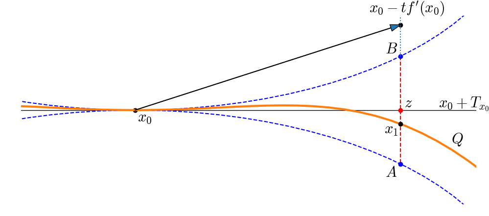
Figure 1. Lemma 1.

We have

(13) $$f(x_{1})-f(x_{0})=f(x_{1})-f(z)+f(z)-f(x_{0}),$$

$\|x_{0}-z\|=t\|P_{T_{x_{0}}}f^{\prime}(x_{0})\|$,

(14) $$\|x_{1}-z\|\leq R-\sqrt{R^{2}-\|x_{0}-z\|^{2}}\leq\frac{\|x_{0}-z\|^{2}}{R}=\frac{t^{2}\|P_{T_{x_{0}}}f^{\prime}(x_{0})\|^{2}}{R}.$$

(15) $$|f(x_{1})-f(z)|\leq L\|x_{1}-z\|\leq\frac{t^{2}L}{R}\|P_{T_{x_{0}}}f^{\prime}(x_{0})\|^{2},$$

and

$$f(z)-f(x_{0})\leq(f^{\prime}(x),z-x_{0})+\frac{L_{1}}{2}\|z-x_{0}\|^{2}=\|P_{T_{x_{0}}}f^{\prime}(x_{0})\|^{2}\left(-t+\frac{L_{1}}{2}t^{2}\right).$$

Substituting the last inequality and (15) in Formula (13) we get (12).∎

Note that if the function $g$ in Lemma 1 has the Lipschitz continuous gradient with Lipschitz constant $L_{1}$ and there exists $m>0$ with $\|g^{\prime}(x)\|\geq m$ for all $x$, $g(x)=0$, then the set $\{x\ |\ g(x)=0\}$ is proximally smooth with constant $R=m/L_{1}$ [36, Proposition 4.15].

Theorem 3.

Suppose that conditions of Lemma 1 hold, $t\in(0,2t_{0})$, and the function $f$ satisfies the LPL condition with constant $\mu>0$ on the set $Q\cap\mathcal{L}_{f}(\beta)$. Then the GPA2 with initial condition $x_{0}\in Q\cap\mathcal{L}_{f}(\beta)$, converges with linear rate to the minimum point.

Proof. Put $\varphi(x)=f(x)-f_{0}$, where $f_{0}=\min_{Q}f$. From the LPL condition for the function $f$ on the surface $Q$

$$\|P_{T_{x}}f^{\prime}(x)\|^{2}\geq\mu(f(x)-f_{0})$$

for all $x\in Q\cap\mathcal{L}_{f}(\beta)$ by Lemma 1 we have

$$f(x_{k+1})-f(x_{k})\leq-q(t)\mu(f(x_{k})-f_{0}),$$

$$\varphi(x_{k+1})\leq(1-q(t)\mu)\varphi(x_{k}).$$

Now consider the rate of convergence with respect to the point. By (14) we get

$$\|x_{k+1}-x_{k}\|^{2}=\|x_{k}-z_{k}\|^{2}+\|z_{k}-x_{k+1}\|^{2}\leq t^{2}\|P_{T_{x_{k}}}f^{\prime}(x_{k})\|^{2}\left(1+\frac{\|P_{T_{x_{k}}}f^{\prime}(x_{k})\|^{2}}{R^{2}}t^{2}\right).$$

Using (12) for $x_{0}=x_{k}$ and $x_{1}=x_{k+1}$ we obtain that

$$\|x_{k+1}-x_{k}\|^{2}\leq\left(1+\frac{L^{2}}{R^{2}}t^{2}\right)\frac{t^{2}}{q(t)}(f(x_{k})-f_{0}),$$

$$\|x_{k+1}-x_{k}\|^{2}\leq\left(1+\frac{L^{2}}{R^{2}}t^{2}\right)\frac{t^{2}}{q(t)}\varphi(x_{k})\leq\left(1+\frac{L^{2}}{R^{2}}t^{2}\right)\frac{t^{2}}{q(t)}(1-q(t)\mu)^{k}\varphi(x_{0}).$$

Due to inequalities for $t,q(t)$ this implies $\|x_{k+1}-x_{k}\|^{2}\leq cp^{k},p<1$. The end of the proof is standard (compare the proof of Theorem 2). ∎

Example 4.

Let $Q$ be a $C^{1}$ and proximally smooth with constant $R$ manifold without edge, $f:\mathbb{R}^{n}\to\mathbb{R}$ be a strongly convex function (with constant of strong convexity $\varkappa>0$) with the Lipschitz continuous gradient. Suppose that $f$ is the Lipschitz function with constant $L>0$ on the level set $\mathcal{L}_{f}(\beta)$ and $\frac{L}{\varkappa}<R$. Then the function $f$ satisfies the LPL condition on the set $Q\cap\mathcal{L}_{f}(\beta)$. We shall give a sketch of proof for this fact.

By [4, Lemma 2.1] the function $f$ has unique minimum $x_{*}\in Q\cap\mathcal{L}_{f}(\beta)$. Fix a point $x_{0}\in Q\cap\mathcal{L}_{f}(\beta)$ and put $z=x_{0}-\tau P_{T_{x_{0}}}f^{\prime}(x_{0})$. Choose a positive number $\tau$ from the conditions of Lemma 1, $\tau$ less than $t$ from [4, Formula (8)] and $\tau\leq\frac{R}{2L}$. Then by strong convexity of the function $f$ by [4] we have linear rate of convergence for the GPA1 with step $\tau$. From Theorem 2.3 [4] for $\overline{x}_{1}=P_{Q}(x_{0}-\tau f^{\prime}(x_{0}))$ we get

$$\|x_{0}-x_{*}\|\leq\sum\limits_{k=0}^{\infty}q^{k}\|x_{0}-\overline{x}_{1}\|\leq\frac{\|x_{0}-\overline{x}_{1}\|}{1-q}$$

where $q=q(\tau)\in(0,1)$ [4, Formula (8)] and $q$ does not depend upon $x_{0}$.

Let $w=P_{x_{0}+T_{x_{0}}}\overline{x}_{1}$, $y=x_{0}-\tau f^{\prime}(x_{0})$. Then from the definition of $\overline{x}_{1}$ we have $\|y-x_{0}\|\geq\|y-\overline{x}_{1}\|$, thus we get the inequality $\|w-z\|\leq\|x_{0}-z\|$. By Formula (14) we obtain that $\|\overline{x}_{1}-w\|\leq\frac{1}{R}\left(2\|x_{0}-z\|\right)^{2}$. Hence by the Pythagoras theorem

$$\|\overline{x}_{1}-z\|^{2}=\|z-w\|^{2}+\|w-\overline{x}_{1}\|^{2}\leq\qquad\qquad\qquad\qquad\qquad\qquad\qquad\qquad\qquad\qquad$$

$$\qquad\qquad\qquad\qquad\qquad\leq\|x_{0}-z\|^{2}+\frac{1}{R^{2}}\left(2\|x_{0}-z\|\right)^{4}\leq\|x_{0}-z\|^{2}\left(1+\frac{4\tau^{2}L^{2}}{R^{2}}\right),$$

(16) $$\|x_{0}-x_{*}\|\leq\frac{\|x_{0}-\overline{x}_{1}\|}{1-q}\leq\frac{\|x_{0}-z\|+\|z-\overline{x}_{1}\|}{1-q}\leq D\|x_{0}-z\|=D\tau\|P_{T_{x_{0}}}f^{\prime}(x_{0})\|,$$

where $D=\left(1+\sqrt{1+\frac{4\tau^{2}L^{2}}{R^{2}}}\right)/(1-q)$.

Suppose that $f^{\prime}(x_{*})\neq 0$. Put $p=\frac{f^{\prime}(x_{*})}{\|f^{\prime}(x_{*})\|}$. By the supporting principle for proximally smooth sets

$$\|x_{*}-x_{0}\pm Rp\|\geq R,$$

$$(p,x_{0}-x_{*})\leq\frac{1}{2R}\|x_{0}-x_{*}\|^{2},\quad(f^{\prime}(x_{*}),x_{0}-x_{*})\leq\frac{\|f^{\prime}(x_{*})\|}{2R}\|x_{0}-x_{*}\|^{2}.$$

In the case $f^{\prime}(x_{*})=0$ the last formula also takes place. From (4) and (16) we obtain that

$$f(x_{0})-f(x_{*})\leq(f^{\prime}(x_{*}),x_{0}-x_{*})+\frac{L_{1}}{2}\|x_{0}-x_{*}\|^{2}\leq\|x_{0}-x_{*}\|^{2}\left(\frac{\|f^{\prime}(x_{*})\|}{2R}+\frac{L_{1}}{2}\right)\leq$$

$$\leq\|x_{0}-x_{*}\|^{2}\left(\frac{L}{2R}+\frac{L_{1}}{2}\right)\leq D^{2}\tau^{2}\left(\frac{L}{2R}+\frac{L_{1}}{2}\right)\|P_{T_{x_{0}}}f^{\prime}(x_{0})\|^{2}.$$

3.5. The gradient method combined with the Newton method on the unit sphere

Describe some symbiosis of the gradient projection algorithm and the Newton method for finding a stationary point for the problem $\min_{Q}f$. We shall assume that $f\in C^{2}$.

Consider again the problem with $Q=S_{1}$. Define $S_{1}$ with the help of the function $g(x)=\frac{1}{2}(\|x\|^{2}-1)=0$. For any $\|x\|=1$ define the number $\lambda\in\mathbb{R}$ as a solution of the extremal problem

$$\|f^{\prime}(x)+\lambda g^{\prime}(x)\|^{2}\to\min\limits_{\lambda},$$

thus $\lambda=-(g^{\prime}(x)^{T}g^{\prime}(x))^{-1}g^{\prime}(x)^{T}f^{\prime}(x)=-(x,f^{\prime}(x))$. Denote by $z$ the variable $(x,\lambda)\in\mathbb{R}^{n+1}$,

$$F(z)=\left[\begin{array}[]{c}f^{\prime}(x)+\lambda x\\ g(x)\end{array}\right],\quad F^{\prime}(z)=\left[\begin{array}[]{cc}f^{\prime\prime}(x)+\lambda I&x\\ x^{T}&0\end{array}\right].$$

Fix $z=(x,\lambda)$, where $x\in S_{1}$, $\lambda=-(x,f^{\prime}(x))$. Define also

$$\sigma_{1}=\arg\min\limits_{\sigma\in\sigma(F^{\prime}(z))}|\sigma|$$

the minimal by absolute value element of spectrum for the matrix $F^{\prime}(z)$.

Suppose that $\sigma_{1}>0$ and $F^{\prime}$ is the Lipschitz continuous with Lipschitz constant $L_{1}>0$ on the set $B_{r}(z)$, where $r=\frac{2}{\sigma_{1}}\|F(z)\|$. Then in the case

(17) $$\frac{L_{1}}{\sigma_{1}^{2}}\sqrt{\|f^{\prime}(x)+\lambda x\|^{2}+g^{2}(x)}=\frac{L_{1}}{\sigma_{1}^{2}}\sqrt{\|f^{\prime}(x)-(x,f^{\prime}(x))x\|^{2}+g^{2}(x)}<\frac{1}{4}$$

the modified Newton method starting from the point $z=(x,-(x,f^{\prime}(x)))$ converges with super-linear rate [21, Chapter X, §4, Theorem 1].

Note that $\|P_{T_{x}}f^{\prime}(x)\|=\|f^{\prime}(x)-(x,f^{\prime}(x))x\|=\|(I-xx^{T})f^{\prime}(x)\|$.

Gradient Projection — Newton Method (GPA3)

Step 1. Take $x_{0}\in{S_{1}}$, and put $C=\frac{\sigma_{1}^{2}}{4L_{1}}$, $k=0$.

Step 2. (GPA2 phase) While $\|P_{T_{x_{k}}}f^{\prime}(x_{k})\|\geq C$, perform Steps 2-4 of GPA2, increasing $k$. If $\|P_{T_{x_{k}}}f^{\prime}(x_{k})\|<C$, proceed to Step 3.

Step 3. Put $x_{0}=x_{k}$, $\lambda_{0}=-(x_{k},f^{\prime}(x_{k}))$, $k=0$.

Step 4. (Newton phase) do Newton steps for equation $F(z)=0$, increasing $k$:

$$\begin{array}[]{rl}\begin{bmatrix}x_{k+1}\\ \lambda_{k+1}\end{bmatrix}&=\begin{bmatrix}x_{k}\\ \lambda_{k}\end{bmatrix}-F^{\prime}\Big{(}\begin{bmatrix}x_{0}\\ \lambda_{0}\end{bmatrix}\Big{)}^{-1}F\Big{(}\begin{bmatrix}x_{k}\\ \lambda_{k}\end{bmatrix}\Big{)}=\\ &=\begin{bmatrix}x_{k}\\ \lambda_{k}\end{bmatrix}-\begin{bmatrix}f^{\prime\prime}(x_{0})+\lambda_{0}I&x_{0}\\ x_{0}^{T}&0\end{bmatrix}^{-1}\begin{bmatrix}f^{\prime}(x_{k})+\lambda_{k}x_{k}\\ g(x_{k})\end{bmatrix}\end{array}$$

Conditions of Lemma 1 are satisfied at Step 2. Thus we can do steps (12) of the GPA2 and decrease the function:

$$f(x_{k+1})-f(x_{k})\leq-C^{2}q(t).$$

Put $\Delta f=\max_{S_{1}}f-\min_{S_{1}}f$. It’s easy to see that by the inequality $\|P_{T_{x_{k}}}f^{\prime}(x_{k})\|\geq C$ we’ll switch to the Newton method at Step 4 after no more than $\frac{\Delta f}{C^{2}q(t)}$ steps of the gradient projection algorithm. In the case when condition (17) is valid at the point $z=(x_{k},-(x_{k},f^{\prime}(x_{k})))$ the modified Newton method starting from $z$ converges with super-linear rate.

3.6. Quadratic form

Consider homogeneous quadratic function $f(x)=(Ax,x)$ with symmetric real $n\times n$ matrix $A$. Denote by $\lambda_{k}$ eigenvalues of $A$, $e_{k}$ — corresponding eigenvectors $Ae_{k}=\lambda_{k}e_{k}$ and suppose that $\lambda_{1}<\lambda_{2}\leq\dots\leq\lambda_{n}$. Then $f_{0}=\lambda_{1},L_{1}=2\lambda_{n}$ and two global minimizers are $\pm e_{1}$. All other eigenvectors are stationary points, but not local minimums. Thus the problem (1) is equivalent to the problem of finding the minimal eigenvalue and eigenvector, and algorithm (6) has the form

(18) $$x_{k+1}=\frac{x_{k}-(2/L_{1})Ax_{k}}{\|x_{k}-(2/L_{1})Ax_{k}\|}.$$

Probably, the first gradient-like algorithm for eigenvalue problem has been proposed by Kantorovich [20, Section 3.4]. He converted eigenvalue problem to unconstrained minimization of Rayleigh quotient $R(x)=\frac{(Ax,x)}{(x,x)}$ and obtained the algorithm $x_{k+1}=\frac{x_{k}-t_{k}Ax_{k}}{\|x_{k}-t_{k}Ax_{k}\|}$ where $t_{k}$ was taken from 1D minimization of $R(x_{k+1})$. One can see that this method has the same form as (18), but has more complicated step-size rule. Kantorovich proved linear convergence of the algorithm.

We analyse iterative process (18) by use of the above presented results. For $x_{0}=\sum_{i=1}^{n}\alpha_{i}e_{i}$ we shall prove convergence to $+e_{1}$ or $-e_{1}$ depending on the sign of $\alpha_{1}$. Suppose that $\alpha_{1}>0$ (if $\alpha_{1}=0$, there is no convergence to global minimum). It is obvious that if $\alpha_{1}>0$, the same is true for decompositions of all iterates $x_{k}$, thus all of them remain in the open half-sphere $H=\{x\ |\ (x,e_{1})>0,||x||=1\}$. We also introduce $H_{\tau}=\{x\ |\ (x,e_{1})\geq\tau,\;||x||=1\},$ for $0<\tau<1$.

Lemma 2.

Fix $\tau\in(0,1)$. Suppose that $\lambda_{1}<\lambda_{2}\leq...\leq\lambda_{n}$ are eigenvalues of $A$. Then the quadratic function $f(x)=(Ax,x)$ satisfies the LPL condition on the set $H_{\tau}$ with $\mu=4\tau^{2}(\lambda_{2}-\lambda_{1})$,

Proof. Express any point $x=\sum_{i=1}^{n}\alpha_{i}e_{i}\in H_{\tau}$ through the residual vector $\delta$: $\delta=x-e_{1}$. From $\tau\in(0,1)$ we have $0<\|\delta\|<\sqrt{2}$. Put $C=\|\delta\|^{2}-\frac{\|\delta\|^{4}}{4}>0$. Using notation $y$ for the unit vector $y=\frac{1}{\sqrt{C}}[\alpha_{2},\alpha_{3},...,\alpha_{n}]^{T}\in\mathbb{R}^{n-1}$ (see (19)), and $B$ for the diagonal matrix with strictly positive diagonal elements

$$B=\begin{bmatrix}\lambda_{2}-\lambda_{1}&0&\cdots&0\\ 0&\lambda_{3}-\lambda_{1}&\cdots&0\\ \vdots&\vdots&\ddots&\vdots\\ 0&0&\cdots&\lambda_{n}-\lambda_{1}\\ \end{bmatrix}$$

we have the next obvious equalities below

$$1=\|x\|^{2}=\sum_{i=1}^{n}\alpha_{i}^{2},\qquad\|\delta\|^{2}=(1-\alpha_{1})^{2}+\sum_{i=2}^{n}\alpha_{i}^{2}=2-2\alpha_{1},$$

(19) $$\sum_{i=2}^{n}\alpha_{i}^{2}=1-\alpha_{1}^{2}=\|\delta\|^{2}-\frac{\|\delta\|^{4}}{4}\doteq C,\qquad(A-\lambda_{1}I)\delta=\sum_{i=2}^{n}(\lambda_{i}-\lambda_{1})\alpha_{i}e_{i},$$

$$\|(A-\lambda_{1}I)\delta\|^{2}=\sum_{i=2}^{n}(\lambda_{i}-\lambda_{1})^{2}\alpha_{i}^{2}=C\|By\|^{2},$$

(20) $$((A-\lambda_{1}I)\delta,\delta)=\sum_{i=2}^{n}(\lambda_{i}-\lambda_{1})\alpha_{i}^{2}=C(By,y),$$

(21) $$f(x)-f_{0}=(Ax,x)-\lambda_{1}=\sum_{i=1}^{n}(\lambda_{i}-\lambda_{1})\alpha_{i}^{2}=\sum_{i=2}^{n}(\lambda_{i}-\lambda_{1})\alpha_{i}^{2}=C(By,y).$$

It is clear that $(By,y)\geq\lambda_{2}-\lambda_{1}>0$.

From the equality $f^{\prime}(x)=2Ax=2A(e_{1}+\delta)$ we get

$$\|(I-xx^{T})f^{\prime}(x)\|^{2}=\|(I-(e_{1}+\delta)(e_{1}+\delta)^{T})(2A(e_{1}+\delta))\|^{2}=$$

$$=4\Big{\|}(A-\lambda_{1}I)\delta+(e_{1}+\delta)(A\delta-\lambda_{1}\delta,\delta)\Big{\|}^{2}=$$

$$=4\|(A-\lambda_{1}I)\delta\|^{2}-4((A-\lambda_{1}I)\delta,\delta)^{2}=$$

$$=4C\|By\|^{2}-4C^{2}(By,y)^{2}=4C(\|By\|^{2}-C(By,y)^{2})=$$

$$=4C(\|By\|^{2}-(By,y)^{2})+4C(1-C)(By,y)^{2}\geq$$

$$\geq 4(1-C)(By,y)\big{[}C(By,y)\big{]}=4(1-C)(By,y)(f(x)-f_{0}).$$

By $4(1-C)=(2-\|\delta\|^{2})^{2}$ the latter expression has the form

$$\|(I-xx^{T})f^{\prime}(x)\|^{2}\geq(2-\|\delta\|^{2})^{2}(\lambda_{2}-\lambda_{1})(f(x)-f(x^{*})).$$

for all $x\in H_{\tau}$. The inequality $2-\|\delta\|^{2}=2-\|x-e_{1}\|^{2}=2(x,e_{1})\geq 2\tau$ holds for $x\in H_{\tau}$, and thus the LPL condition takes place with $\mu=4\tau^{2}(\lambda_{2}-\lambda_{1})$.∎

Thus for any $(x_{0},e_{1})\geq\tau$ we get $(Ax_{k},x_{k})-\lambda_{1}\leq((Ax_{0},x_{0})-\lambda_{1})q^{k},q=1-\tau^{2}\frac{\lambda_{2}-\lambda_{1}}{\lambda_{n}-\lambda_{1}}$ (denominator $\|Lx_{k}-f^{\prime}(x_{k})\|$ from (11) is bounded from above by $2(\lambda_{n}-\lambda_{1})$ for the quadratic function), while asymptotically $|(x_{k},e_{1})|\rightarrow 1$, and $(Ax_{k},x_{k})-\lambda_{1}=O(q_{1}^{k}),\;q_{1}=\frac{\lambda_{n}-\lambda_{2}}{\lambda_{n}-\lambda_{1}}$.

Condition $\lambda_{1}<\lambda_{2}\dots$ can be weakened. If $\lambda_{1}=\dots=\lambda_{k}<\lambda_{k+1}\leq\dots\leq\lambda_{n}$, then the function $f(x)=(Ax,x)$ also satisfies the LPL condition on the set $H_{\tau}=\{x\in S_{1}\ |\ \sum_{i=1}^{k}x_{i}^{2}\geq\tau^{2}\}$ of the unit sphere $S_{1}$ for any $\tau\in(0,1)$ in the basis from eigenvectors.

Indeed, put $z=(x_{1},\dots,x_{k})$, $\overline{x}=(x_{k+1},\dots,x_{n})$, $x=(z,\overline{x})$. Then

$$f(x)=\sum\limits_{i=1}^{n}\lambda_{i}x_{i}^{2}=\lambda_{1}\|z\|^{2}+\sum\limits_{i=k+1}^{n}\lambda_{i}x_{i}^{2}=h(\|z\|,\overline{x}).$$

For the function $h(\|z\|,\overline{x})$ we have the LPL condition on the set $\{\|z\|>\tau\}$ with constant $\mu=4\tau^{2}(\lambda_{k+1}-\lambda_{1})$, i.e.

$$4\left(\lambda_{1}^{2}\|z\|^{2}+\sum\limits_{i=k+1}^{n}\lambda_{i}x_{i}^{2}\right)\geq\mu(h(z,\overline{x})-f_{0}),$$

or equivalently

$$4\left(\sum\limits_{i=1}^{n}\lambda_{i}x_{i}^{2}\right)\geq\mu(f(x)-f_{0}).$$

4. The Frank-Wolfe method

The Frank-Wolfe method (also known as the conditional gradient method) has been proposed for minimization of a convex quadratic function on a convex set [15] and later was extended for general convex objectives, see e.g. [31] and recent survey [14]. The idea of the method for problem (1) is to solve (on each step) the auxiliary problem

$$z_{k}\in\mbox{\rm Arg}\min\limits_{z\in Q}(f^{\prime}(x_{k}),z),$$

find $t\in[0,1]$ that minimizes $f(x_{k}+t(z_{k}-x_{k}))$ and take the next point $x_{k+1}=x_{k}+t(z_{k}-x_{k})$. The method requires minimization of a linear function on the admissible set at each iteration. There are also some extensions of the method for nonconvex objective functions and for matrix optimization [26, 37].

4.1. Minimization of an approximately linear function

However our problem (1) deals with non-convex admissible set $Q$. We consider a special version of the FW method for our problem as a limiting version of the gradient projection method (6). Indeed suppose that the function $f(x)$ is approximately linear (see (23) below) on the set $Q=S_{1}$, i.e., informally, constant $L_{1}$ is small enough in comparison with other parameters. For this extreme case method (6) turns into the next iteration process

(22) $$x_{k+1}=-\frac{f^{\prime}(x_{k})}{\|f^{\prime}(x_{k})\|}.$$

This is exactly the FW method with $t=1$: we take linearized function $f(x_{k})+(f^{\prime}(x_{k}),x-x_{k})$, find its minimum on $Q$ and proceed to the minimum point. Notice that in standard versions of the FW method we make a step in the direction of the minimizer; this full-step version diverges in general case.

Full-step Frank-Wolfe method (FFW)

Step 1. Take $x_{0}$ and set $k=0$.

Step 2. Solve auxiliary problem

$$z_{k}\in\mbox{\rm Arg}\min\limits_{z\in Q}(f^{\prime}(x_{k}),z),$$

Step 3. Update $x_{k+1}=z_{k}.$

Step 4. Increase $k$ and go to Step 2.

To get the rigorous validation of method (22) we need specification of the above mentioned approach. A function $f(x)$ defined on the ball $B_{1}(0)$ with $L_{1}$-Lipschitz gradient (3) is called approximately linear on $S_{1}$ if

(23) $$||f^{\prime}(0)||>2L_{1}.$$

Theorem 4.

Suppose that (23) holds. There are just two stationary points in problem (1) $x_{*}=\arg\min_{S_{1}}f(x),$ $x^{*}=\arg\max_{S_{1}}f(x)$, and FFW method (22) converges to $x_{*}$ for arbitrary $x_{0}\in S_{1}$ with linear rate

(24) $$||x_{k}-x_{*}||\leq q^{k}||x_{0}-x_{*}||,\quad q=\frac{L_{1}}{\|f^{\prime}(0)\|-L_{1}}\in(0,1).$$

Theorem 4 is close enough to Theorem 4.3 from [32] where minimization on $B_{1}$ instead of $S_{1}$ has been considered. But indeed the solutions of these two problems coincide under condition (24). The proof of Theorem 4 follows from the following fact regarding strongly convex sets of radius $r$ and functions with the Lipschitz continuous gradient [3].

Suppose that $B\subset\mathbb{R}^{n}$ is a strongly convex set of radius $r$ and a function $f:\mathbb{R}^{n}\to\mathbb{R}$ has the Lipschitz continuous gradient with constant $L_{1}$, $m=\inf\limits_{x\in\partial Q}\|f^{\prime}(x)\|$ and $\frac{m}{L_{1}}>r$. Then the iteration process $x_{0}\in\partial B$,

$$x_{k+1}=\arg\min\limits_{x\in B}(f^{\prime}(x_{k}),x),\qquad k=0,1,\dots$$

converges to the unique solution $x_{*}\in\partial B$ of the problem $\min_{B}f$ with linear rate:

$$\|x_{k}-x_{*}\|\leq\left(\frac{rL_{1}}{m}\right)^{k}\|x_{0}-x_{*}\|.$$

We shall further consider a closed surface $Q$ in $\mathbb{R}^{n}$ which is the boundary of some strongly convex set of radius $r$, i.e. $Q=\partial B$. It is worth to admit that $Q$ is not necessary smooth.

4.2. Another gradient domination condition

We introduce a sort of the gradient domination condition, formulated at a stationary point $x_{*}$ of (1). Assume that the next inequality

(25) $$||f^{\prime}(x_{*})||>L_{1}$$

holds. This condition reminds sharp minimum condition [31].

Theorem 5.

Let $B\subset\mathbb{R}^{n}$ be a strongly convex set of radius $r$, $m>1$, $x_{*}\in\partial B$. Suppose that $f:\mathbb{R}^{n}\to\mathbb{R}$ is a function with the Lipschitz continuous gradient with constant $L_{1}$. If $f^{\prime}(x_{*})\in-N(B,x^{*})$ and $\|f^{\prime}(x_{*})\|\geq mrL_{1}$ then $x_{*}=\arg\min\limits_{a\in B}f(a)$, i.e. $x_{*}$ is the strict global minimum of the function $f$ on the set $B$, and hence on the boundary $Q=\partial B$.

Proof. Put $p=\frac{f^{\prime}(x_{*})}{\|f^{\prime}(x_{*})\|}$. Then by the supporting principle for strongly convex sets

(26) $$B\subset B_{r}(x_{*}+rp).$$

Fix a number $\varepsilon>0$ and a unit vector $q$ such that

(27) $$x=x_{*}+\varepsilon q\in B_{r}(x_{*}+rp).$$

We claim that $f(x)>f(x_{*})$.

By Formula (4)

(28) $$f(x)\geq f(x_{*})+(f^{\prime}(x_{*}),x-x_{*})-\frac{L_{1}}{2}\|x-x_{*}\|^{2}.$$

From (27) we get $\|rp-\varepsilon q\|\leq r$. Hence $-2r\varepsilon(p,q)+\varepsilon^{2}\leq 0$ or $\frac{\varepsilon}{2}\leq r(p,q)$. By inequality $m>1$ we obtain that

(29) $$\frac{\varepsilon}{2}\leq mr(p,q).$$

Further

$$(f^{\prime}(x_{*}),x-x_{*})=(f^{\prime}(x_{*}),\varepsilon q)\geq\varepsilon mrL_{1}(p,q)$$

and $\|x-x_{*}\|^{2}=\varepsilon^{2}$. The last two formulae and (28) gives the next estimate

$$f(x)\geq f(x_{*})+\varepsilon mrL_{1}(p,q)-\frac{L_{1}}{2}\varepsilon^{2}=f(x_{*})+\varepsilon L_{1}\left(mr(p,q)-\frac{\varepsilon}{2}\right),$$

and taking in mind (29) we have $f(x)>f(x_{*})$. By inclusions (26), (27) $x_{*}=\arg\min\limits_{a\in B}f(a)$.∎

Corollary 1.

If $m=1$ and other assumptions of Theorem 5 hold then $x^{*}$ is also a global minimum of $f$ on the set $B$, but this minimum is not necessary strict.

The particular example is given by the set $B=B_{1}(0)$ and the function $f(x)=-\frac{1}{2}\|x\|^{2}$.

Corollary 2.

If in Theorem 5 $m\in(0,1)$ and other assumptions of Theorem 5 hold then $x_{*}$ is a stationary point of the function $f$ on the set $B$ but not necessarily the minimum point.

Example 5.

Consider an example in $\mathbb{R}^{2}$. Fix $r>1$, let $B=\{(x,y)\in R^{2}\ |\ x^{2}+(y+r)^{2}\leq r^{2}\}=B_{r}((0,-r))$.

Define the function $\psi$

$$\psi(x)=\left\{\begin{array}[]{c}-\frac{1}{2}x^{2},\quad x\leq 0,\\ 0,\quad x>0,\\ \end{array}\right.\qquad\psi^{\prime}(x)=\left\{\begin{array}[]{c}-x,\quad x\leq 0,\\ 0,\quad x>0\\ \end{array}\right.$$

and $f(x,y)=\psi(x)-y$ for all $(x,y)\in\mathbb{R}^{2}$.

Consider the problem $\min_{B}f$. We have $f^{\prime}(x,y)=(\psi^{\prime}(x),-1)$ and thus $f^{\prime}$ is the Lipschitz continuous with constant $L_{1}=1$.

The point $a=(0,0)\in\partial B$ is a stationary point: $f^{\prime}(a)=(0,-1)\in-N(B,a)$, $\|f^{\prime}(a)\|=1=mrL_{1}=mr$, i.e. $m=\frac{1}{r}<1$ and $f(a)=0$. But $a$ is not a local minimum. The solution of the problem is $a_{0}=(-\sqrt{r^{2}-1},1-r)$ with $f(a_{0})=-\frac{(r-1)^{2}}{2}$.∎

Define the function $h(\theta)=2\sin\left(\frac{1}{2}\arcsin\theta\right)$ for $\theta\in[0,1]$. The function $h$ is convex, monotonically increasing and $\frac{1}{\theta}h(\theta)>1$ for $\theta>0$. By convexity of $h$ we have for any $t\in(0,\theta)$ that $h(t)\leq\frac{1}{\theta}h(\theta)t$. Note that $1\leq\frac{1}{\theta}h(\theta)\leq\sqrt{2}$ if $\theta\in[0,1]$.

For any real number $m>1$ define $\theta_{m}$ as follows

$$\theta_{m}=\left\{\begin{array}[]{lc}\theta,\quad\mbox{where}\ \frac{1}{\theta}h(\theta)=m\ \mbox{and}\ m\in(1,\sqrt{2}],\\ 1,\ m>\sqrt{2}.\end{array}\right.$$

Theorem 6.

Let $B\subset\mathbb{R}^{n}$ be a strongly convex set of radius $r$, $m>1$, $x_{*}\in\partial B$. Suppose that $f:\mathbb{R}^{n}\to\mathbb{R}$ is a function with the Lipschitz continuous gradient with constant $L_{1}$, $f^{\prime}(x_{*})\in-N(B,x_{*})$ and $\|f^{\prime}(x_{*})\|\geq mrL_{1}$. Fix a point $x_{0}\in\partial B$, $\|x_{0}-x_{*}\|<\theta mr$ and $\theta\in(0,\theta_{m})$. Then the iterations

$$x_{k+1}=\arg\max\limits_{x\in\partial B}(-f^{\prime}(x_{k}),x),\quad k=0,1,\dots$$

of FFW method converge to the point $x_{*}$ with linear rate:

$$\|x_{k+1}-x_{*}\|\leq\frac{1}{\theta}\frac{h(\theta)}{m}\|x_{k}-x_{*}\|$$

for all $k$.

Note that by Theorem 5 $x_{*}$ is the strict global minimum of $f$ on the set $B$. Also $\frac{1}{\theta}\frac{h(\theta)}{m}<1$ due to choice of $\theta$.

Proof. Put $t_{k}=\|x_{k}-x_{*}\|$.

From the inequality $L_{1}t_{k}<\|f^{\prime}(x_{*})\|$ (which follows by induction) and the inclusion $f^{\prime}(x_{k})\in B_{L_{1}t_{k}}(f^{\prime}(x_{*}))$ the sine of the angle $\varphi_{k}$ between $f^{\prime}(x_{*})$ and $f^{\prime}(x_{k})$ is estimated as follows

$$\sin\varphi_{k}\leq\frac{L_{1}t_{k}}{\|f^{\prime}(x_{*})\|}\leq\frac{t_{k}}{mr}.$$

Put $p_{k}=-\frac{f^{\prime}(x_{k})}{\|f^{\prime}(x_{k})\|}$, $p_{*}=-\frac{f^{\prime}(x_{*})}{\|f^{\prime}(x_{*})\|}$. From the triangle $0p_{k}p_{*}$ we have $\|p_{k}-p_{*}\|=2\sin\frac{1}{2}\varphi_{k}$. By strong convexity of the set $B$ and inequality $\frac{t_{k}}{mr}<\theta$ we obtain that

$$t_{k+1}=\|x_{k+1}-x_{*}\|\leq r\|p_{k}-p_{*}\|=2r\sin\frac{1}{2}\varphi_{k}\leq 2r\sin\left(\frac{1}{2}\arcsin\frac{t_{k}}{mr}\right)\leq\frac{1}{\theta}\frac{h(\theta)}{m}t_{k}.$$

∎

Theorem 7.

Let $B\subset\mathbb{R}^{n}$ be a strongly convex set of radius $r$, $m>1$, $\beta\in\mathbb{R}$. Suppose that $f:\mathbb{R}^{n}\to\mathbb{R}$ is a function with the Lipschitz continuous gradient with constant $L_{1}$ and for any point $x\in\partial B\cap\mathcal{L}_{f}(\beta)$ we have the inequality $\|f^{\prime}(x)\|\geq mrL_{1}$. Then for any choice of the initial point $x_{0}\in\partial B\cap\mathcal{L}_{f}(\beta)$ the iterations

$$x_{k+1}=\arg\max\limits_{x\in\partial B}(-f^{\prime}(x_{k}),x),\quad k=0,1,\dots$$

converge to the global strict minimum $x_{*}$ with linear rate:

$$\|x_{k+2}-x_{k+1}\|\leq\frac{1}{m}\|x_{k+1}-x_{k}\|.$$

for all $k$.

Proof. Put $t_{k}=\|x_{k+1}-x_{k}\|$ and $p_{k}=-\frac{f^{\prime}(x_{k})}{\|f^{\prime}(x_{k})\|}$.

Suppose that $f(x_{i})\leq\beta$ for all $0\leq i\leq k$.

Prove that $f(x_{k+1})\leq\beta$.

$$f(x_{k+1})-f(x_{k})\leq(f^{\prime}(x_{k}),x_{k+1}-x_{k})+\frac{L_{1}}{2}\|x_{k+1}-x_{k}\|^{2}.$$

From the supporting principle for strongly convex sets

$$\|x_{k+1}-rp_{k}-x_{k}\|<r,$$

or

$$\|x_{k+1}-x_{k}\|^{2}\leq 2r(p_{k},x_{k+1}-x_{k})\leq-\frac{2}{mL_{1}}(f^{\prime}(x_{k}),x_{k+1}-x_{k}).$$

Hence we obtain the next estimate

$$f(x_{k+1})-f(x_{k})\leq-\left(m-1\right)\frac{L_{1}}{2}\|x_{k+1}-x_{k}\|^{2},$$

and $f(x_{k+1})\leq f(x_{k})\leq\beta$.

For any unit vectors $p,q$ and numbers $\lambda,\mu\geq 1$ we have $\|p-q\|\leq\|\lambda p-\mu q\|$. Using the last inequality and strong convexity of the set $B$ we get

$$t_{k+1}=\|x_{k+2}-x_{k+1}\|\leq r\left\|\frac{f^{\prime}(x_{k+1})}{mrL_{1}}-\frac{f^{\prime}(x_{k})}{mrL_{1}}\right\|\leq\frac{1}{m}t_{k}.$$

Thus the sequence $\{x_{k}\}$ converges, $x_{k}\to x_{*}\in\partial B$. Passing to the limit as $k\to\infty$ in the inclusion $-f^{\prime}(x_{k})\in N(B,x_{k+1})$ and using upper semicontinuity of the normal cone we have $-f^{\prime}(x_{*})\in N(B,x_{*})$, $\|f^{\prime}(x_{*})\|\geq mrL_{1}$. By Theorem 5 the point $x_{*}$ is the strict global minimum. ∎

Consider examples that show importance of the condition $m>1$ in both Theorems 6 and 7.

Example 6.

Suppose that $f(x,y)$ and $B$ are the function and the set from Example 5. Notice that in this case $m<1$. Take a starting point for the FFW algorithm $(x_{0},y_{0})\in\partial B$ with $x_{0}>0$, $y_{0}\in(-1,0)$. Then $f^{\prime}(x_{0},y_{0})=(0,-1)$ and one step of the FFW method leads us to the stationary point $(0,0)$. But extremum is the point $(-\sqrt{r^{2}-1},1-r)$, see Figure 2.

Figure 2. Stationary point $(0,0)$ is not a solution.

Example 7.

Consider the set $Q=\{(x,y)\in\mathbb{R}^{2}\ |\ x^{2}+(y-\frac{1}{2})^{2}=\frac{1}{4}\}$. Let $f(x,y)=y-x^{2}$. For the function $f$ we have $L_{1}=2$, $1=\|f^{\prime}(0,0)\|=mrL_{1}=m\frac{1}{2}\cdot 2=m$, i.e. $m=1$,

$$(0,0)=\arg\min\limits_{(x,y)\in Q}f(x,y)$$

and $f_{0}=f(0,0)=0$. Put $t>0$ and $a_{0}=(x_{0},y_{0})\in Q$, $x_{0}>0$, $y_{0}\in(0,\frac{1}{2})$ with $f(x_{0},y_{0})=y_{0}-x_{0}^{2}=t$. As we’ve seen at subsection 3.2 the angle between tangent lines to the circle $Q$ and curve $f(x,y)=y-x^{2}=t$ at the point $a_{0}$ asymptotically equals $x_{0}^{3}$ when $x_{0}\to 0$. Starting the FFW algorithm from the point $a_{0}$ we obtain the next point $a_{1}(x_{1},y_{1})$. We have $x_{0}^{3}\asymp\|a_{0}-a_{1}\|\asymp|x_{0}-x_{1}|$ when $x_{0}\to 0$. The last means that

$$\exists\delta>0\ \exists C>0\ \forall x_{0}\in(0,\delta)\ |x_{0}-x_{1}|<Cx_{0}^{3}.$$

Thus for any sufficiently small $x_{0}>0$ we get $x_{1}\geq x_{0}-Cx_{0}^{3}$. There is no linear rate of convergence.

5. Appendix

Proposition 1.

Suppose that the set $Q\subset\mathbb{R}^{n}$ is proximally smooth with constant $R>0$, the function $f$ has the Lipschitz continuous gradient $f^{\prime}$ with constant $L_{1}>0$ and the point $x_{0}$ is a local minimum in the problem $\min_{Q}f$. Then $-f^{\prime}(x_{0})\in N(Q,x_{0})$.

Proof. If $f^{\prime}(x_{0})=0$ then $-f^{\prime}(x_{0})=0\in N(Q,x_{0})$ by the definition of normal cone.

Assume that $f^{\prime}(x_{0})\neq 0$. Prove the proposition by contradiction. Put $p=-\frac{f^{\prime}(x_{0})}{\|f^{\prime}(x_{0})\|}$. Suppose that $p\notin N(Q,x_{0})$. Then by the supporting principle for a proximally smooth set we have

$$\exists x_{1}\in Q\cap\mbox{\rm int}\,B_{R}(x_{0}+Rp).$$

For a set $B$ define by $D_{R}B$ the intersection of all closed balls of radius $R$ each of which contains the set $B$. From [6, Lemmata 4.13, 4.16] there exists a continuous curve $\Gamma\subset Q$ with endpoints $x_{0}$ and $x_{1}$ such that $\Gamma\subset D_{R}\{x_{1},x_{0}\}\subset\{x_{0}\}\cup\mbox{\rm int}\,B_{R}(x_{0}+Rp)$. By the inclusion $x_{1}\in\mbox{\rm int}\,B_{R}(x_{0}+Rp)$ there exists $\delta>0$ with $B_{\delta}(x_{1})\subset\mbox{\rm int}\,B_{R}(x_{0}+Rp)$,

$$D_{R}\{x_{1},x_{0}\}\subset D_{R}(B_{\delta}(x_{1})\cup\{x_{0}\}).$$

Let $L$ be a 2-dimensional plane, $\{x_{0},x_{1}\}\subset L$. Choose a point $x\in\Gamma$, $\|x-x_{0}\|=\varepsilon$, $x=x_{0}+\varepsilon q$, $\|q\|=1$. The angle $\varphi$ between arcs $L\cap\partial D_{R}\{x_{1},x_{0}\}$ and $L\cap\partial D_{R}(B_{\delta}(x_{1})\cup\{x_{0}\})$ at the point $x_{0}$ (see Figure 3) is strictly positive and hence the angle between $p$ and $q$ is less than $\frac{\pi}{2}-\varphi\in(0,\frac{\pi}{2})$. Thus there exists $C=\cos\left(\frac{\pi}{2}-\varphi\right)>0$ (that does not depend on vector $q$) with $(p,q)>C$.

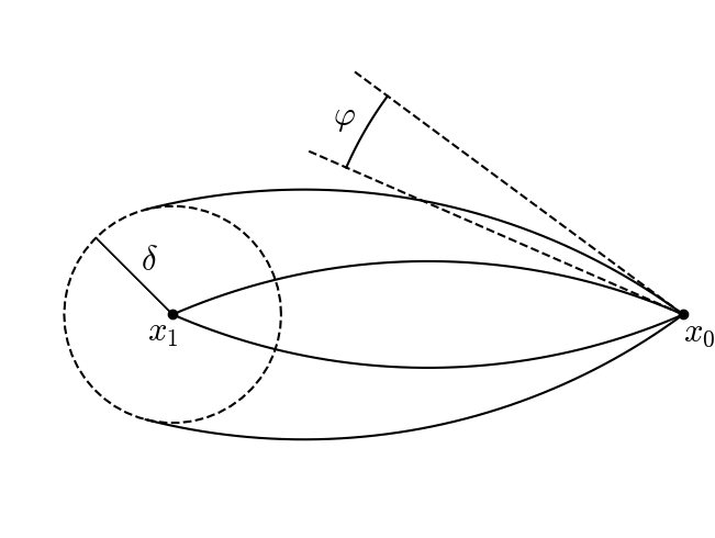
Figure 3. Angle $\varphi$.

By Formula (4)

$$f(x)-f(x_{0})\leq(f^{\prime}(x_{0}),x-x_{0})+\frac{L_{1}}{2}\|x-x_{0}\|^{2}$$

and

$$(f^{\prime}(x_{0}),x-x_{0})=(f^{\prime}(x_{0}),\varepsilon q)=-\|f^{\prime}(x_{0})\|\varepsilon(p,q).$$

Hence

$$f(x)-f(x_{0})\leq-\|f^{\prime}(x_{0})\|\varepsilon(p,q)+\frac{L_{1}}{2}\varepsilon^{2}\leq-\|f^{\prime}(x_{0})\|\varepsilon C+\frac{L_{1}}{2}\varepsilon^{2}<0$$

for sufficiently small $\varepsilon>0$. A contradiction.∎

References

• [1] P.-A. Absil, R. Mahony, R. Sepulchre, Optimization Algorithms on Matrix Manifolds, Princeton University Press, Princeton and Oxford, 2008.
• [2] M. V. Balashov, Uniformly convex subsets of the Hilbert space with modulus of convexity of the second order, Journal of Math. Anal. Appl., 377:2 (2011), 754–761.
• [3] M. V. Balashov, Maximization of a function with Lipschitz continuous gradient, Journal of Mathematical Sciences, 209:1, (2015), 12–18.
• [4] M. V. Balashov, About the gradient projection algorithm for a strongly convex function and a proximally smooth set, Journal of Convex Analysis, 24:2, (2017), 493–500.
• [5] M. V. Balashov, E. S. Polovinkin, M-strongly convex subsets and their generating sets, Sbornik: Mathematics, 191:1 (2000), 25–60.
• [6] M. V. Balashov, G. E. Ivanov, Weakly convex and proximally smooth sets in Banach spaces, Izv. RAN. Ser. Mat., 73:3 (2009), 23–66.
• [7] D. Bertsekas, Mathematical Programming, Athena-Publishing, 2013.
• [8] S. Boyd, L. Vanderberghe, Convex Optimization, Cambridge University Press, 2004.
• [9] F. H. Clarke, Yu. S. Ledyaev, R. J. Stern, P. R. Wolenski, Nonsmooth Analysis and Control Theory, Springer-Verlag New-York Inc., 1998.
• [10] F. H. Clarke, R. J. Stern, P. R. Wolenski, Proximal smoothness and lower–$C^{2}$ property, J. Convex Anal., 2:1-2 (1995), 117–144.
• [11] A. R. Conn, N. I. M. Gould, Ph. L. Toint, Trust-Region Methods, SIAM, Philadelphia, 2000.
• [12] C. Fraikin, Yu. Nesterov, P. Van Dooren, A gradient-type algorithm optimizing the coupling between matrices, Linear Algebra and its Applications, 429 (2008), 1229–1242.
• [13] O. P. Ferreira, A. N. Iusem, and S. Z. Németh, Concepts and techniques of optimization on the sphere, TOP, 22:3 (2014), 1148–1170.
• [14] R. M. Freund, P. Grigas, New analysis and results for the Frank-Wolfe method, Mathem. Progr., 155:1-2 (2016), 199–230.
• [15] M. Frank, Ph. Wolfe, Algorithm for quadratic programming, Nav. Res. Log. Quart., 3:1-2 (1956), 95–110.
• [16] W. W. Hager, Minimizing a quadratic over a sphere, SIAM J. Optim. and Contr., 12:1 (2001), 188–208.
• [17] B. Gao, X. Liu, X. Chen, Ya. Yuan, On the Lojasiewicz exponent of the quadratic sphere constrained optimization problem, (2016), arXiv:1611.08781v2
• [18] A. A. Goldstein, Convex programming in Hilbert space, Bull. Amer. Math. Soc., 70:5 (1964), 709-710.
• [19] H. Karimi, J. Nutini, M. Schmidt, Linear convergence of gradient and proximal-gradient methods under the Polyak-Lojasiewicz condition. In: Frasconi P., Landwehr N., Manco G., Vreeken J. (eds) Machine Learning and Knowledge Discovery in Databases. Lecture Notes in Computer Science, vol 9851. Springer, 2016.
• [20] L. V. Kantorovich, Functional analysis and applied mathematics, Russ. Math. Surveys, 3:6(28) (1948), 89–185.
• [21] A. N. Kolmogorov, S. V. Fomin, Elements of the Theory of Functions and Functional Analysis, Dover Publications, 1999.
• [22] E. S. Levitin, B. T. Polyak, Constrained minimization methods, USSR Comp. Math. and Math. Phys., 6:5 (1966), 787–823.
• [23] T. Ležanski, Über das Minimumproblem von Funktionalen in Banachschen Räumen, Bull. Acad. Pol. Sci., Sér. Sci. Math. Astron. Phys., 10 (1962), 107–110.
• [24] T. Ležanski, Über das Minimumproblem für Funktionale in Banachschen Räumen, Mathematische Annalen, 152 (1963), 271–274.
• [25] D. G. Luenberger, The gradient projection methods along geodesics, Management Science, 18:11 (1972), 620–631.
• [26] S. Lacoste-Julien, Convergence rate of Frank-Wolfe for non-convex objectives, (2016), arXiv:1607.00345
• [27] S. Lojasiewicz, Une propriet e topologique des sous-ensembles analytiques reels, Les Equations aux Derivees Partielles, CNRS, Paris, (1963), 87–89.
• [28] J.X. da Cruz Neto, L. L. De Lima, P. R. Oliveira, Geodesic algorithms on Riemannian manifolds, Balkan J. of Geom. and its Appl., 3:2 (1998), 89–100.
• [29] Yu. Nesterov, Lectures on Convex Optimization, Springer, 2018.
• [30] Yu. Nesterov, A. Nemirovski Interior-point Polynomial Algorithms in Convex Programming, SIAM, 1994.
• [31] B. T. Polyak, Introduction to Optimization. New York, Optimization Software, 1987.
• [32] B. T. Polyak, Local programming, USSR Computational Mathematics and Mathematical Phys. 41:9 (2001), 1259–1266.
• [33] B. T. Polyak, Gradient Methods for the minimization of functionals, USSR Comp. Math. and Math. Phys., 3:4 (1963), 643–653.
• [34] B. T. Polyak, Existence theorems and convergence of minimizing sequences for extremal problems with constraints, Soviet Math. Dokl., 1966, 7, 72–75.
• [35] C. Udrişte, Convex Functions and Optimization Methods on Riemannian Manifolds, Mathematics and Its Applications series, vol. 297, Springer, 1994.
• [36] J.-Ph. Vial, Strong and weak convexity of sets and functions, Mathematics of Operations Research, 8:2 (1983), 231–259.
• [37] M. Weber, S. Sra, Riemannian Frank-Wolfe with application to the geometric mean of positive definite matrices, (2018), arXiv:1710.10770v2