Similarity of thermodynamic properties of Heisenberg model on triangular and kagome lattices

Abstract

Derivation of a reduced effective model allows for a unified treatment and discussion of the $J_{1}$-$J_{2}$ $S=1/2$ Heisenberg model on triangular and kagome lattice. Calculating thermodynamic quantities, i.e. the entropy $s(T)$ and uniform susceptibility $\chi_{0}(T)$, numerically on systems up to effectively $N=42$ sites, we show by comparing to full-model results that low-$T$ properties are qualitatively well represented within the effective model. Moreover, we find in the spin-liquid regime similar variation of $s(T)$ and $\chi_{0}(T)$ in both models down to $T\ll J_{1}$. In particular, studied spin liquids appear to be characterized by Wilson ratio vanishing at low $T$, indicating that the low-lying singlets are dominating over the triplet excitations.

I Introduction

Studies of possible quantum spin-liquid (SL) state in spin models on frustrated lattices have a long history, starting with the Anderson’s conjecture Anderson (1973) for the Heisenberg model on a triangular lattice. In last two decades theoretical efforts have been boosted by the discovery of several classes of insulators with local magnetic moments Lee (2008); Balents (2010); Savary and Balents (2017), which do not reveal long-range order (LRO) down to lowest temperatures $T$. The first class are compounds, as the herbertsmithite ZnCu₃(OH)₆Cl₂ Norman (2016), which can be represented with Heisenberg $S=1/2$ model on kagome lattice, being the subject of numerous experimental studies Mendels et al. (2007); Olariu et al. (2008); Han et al. (2012); Fu et al. (2015), now including also related materials Hiroi et al. (2001); Fåk et al. (2012); Li et al. (2014); Gomilšek et al. (2016); Feng et al. (2017); Zorko et al. (2019) confirming the SL properties, at least in a wide $T>0$ range. Another class are organic compounds, as $\kappa$-(ET)₂Cu₂(CN)₃ Shimizu et al. (2003, 2006); Itou et al. (2010); Zhou et al. (2017), where the spins reside on a triangular lattice. Recently, the charge-density-wave system 1T-TaS₂, which is a Mott insulator without magnetic LRO and shows spin fluctuations at $T>0$ Klanjšek et al. (2017); Kratochvilova et al. (2017); Law and Lee (2017); He et al. (2018), has been added into this family.

Numerical Bernu et al. (1994); Capriotti et al. (1999); White and Chernyshev (2007) and analytical Chernyshev and Zhitomirsky (2009) studies of the nearest-neighbor (nn) quantum $S=1/2$ Heisenberg model (HM) on a triangular lattice (TL) confirm a spiral long-range order (LRO) with spins pointing in $120^{\circ}$ tilted directions. Introducing the next-nearest-neighbor (nnn) coupling $J_{2}>0$ enables the SL ground state (g.s.) in the part of the phase diagram Kaneko et al. (2014); Watanabe et al. (2014); Zhu and White (2015); Hu et al. (2015); Iqbal et al. (2016); Wietek and Läuchli (2017); Gong et al. (2017); Ferrari and Becca (2019). There is even more extensive literature on the HM on the kagome lattice (KL) confirming the absence of g.s. LRO order Mila (1998); Budnik and Auerbach (2004); Iqbal et al. (2011); Läuchli et al. (2011); Iqbal et al. (2013). The prevailing conclusion of numerical studies of the g.s. and lowest excited states is that HM on KL has a finite spin triplet gap $\Delta_{t}$ Yan et al. (2008); Läuchli et al. (2011); Depenbrock et al. (2012); Läuchli et al. (2019) (with some evidence pointing also to gapless SL Iqbal et al. (2013); Liao et al. (2017); Chen et al. (2018)), but much smaller or vanishing singlet gap $\Delta_{s}\ll\Delta_{t}$ Elstner and Young (1994); Mila (1998); Sindzingre et al. (2000); Misguich and Sindzingre (2007); Bernu and Lhuillier (2015); Läuchli et al. (2019); Schnack et al. (2018). On the other hand, extensions into the $J_{1}$-$J_{2}$ model Kolley et al. (2015); Liao et al. (2017) with $J_{2}>0$ again leads towards g.s. with magnetic LRO. Still, HM on both lattices in their respective SL parameter regimes have been studied and considered separately, not recognizing or stressing their similarity.

Our goal is to put extended $J_{1}$-$J_{2}$ HM on TL and KL on a common ground, stressing the similarity of their (in particular thermodynamic) properties within their presumable SL regimes. To this purpose we derive and employ a reduced effective model (EM), which is based on keeping only the lowest four $S=1/2$ states in a single triangle. Such an EM has been previously introduced and analyzed for the case of KL Subrahmanyam (1995); Mila (1998); Budnik and Auerbach (2004); Capponi et al. (2004) and as the starting point for block perturbation approach also for the TL Subrahmanyam (1995), but so far has not been used to evaluate and capture $T>0$ properties. Such an EM has an evident advantage of reduced number of states in an exact-diagonalization (ED) study and hence allowing for somewhat larger lattices (in our study up to $N=42$ sites). Still, this is not the most important message, since EM allows also an insight into the character of low-energy excitations, being now separated into spin (triplet) and chirality (singlet) ones. The main focus of this work is on the numerical evaluation of thermodynamic quantities and their understanding, whereby we do not resort to perturbative limits (extreme breathing limit) of weakly coupled triangles Repellin et al. (2017); Iqbal et al. (2018) which apparently does not represent fully the same SL physics. We concentrate on the entropy density $s(T)$ and uniform susceptibility $\chi_{0}(T)$ within the SL parameter regimes, approached before mostly by high-$T$ expansion Elstner et al. (1993); Elstner and Young (1994); Sindzingre et al. (2000); Misguich and Sindzingre (2007); Rigol et al. (2007); Rigol and Singh (2007); Bernu and Lhuillier (2015); Bernu et al. and only recently with numerical methods adequate for lower $T\ll J_{1}$, both on TL Prelovšek and Kokalj (2018) and KL Chen et al. (2018); Schnack et al. (2018). However, the most universal property is the temperature-dependent Wilson ration $R(T)$, introduced and discussed further on.

I.1 Generalised Wilson ratio

Our results in the following reveal that in both lattices and within the SL regime $s(T)$ and $\chi_{0}(T)$ are very similar in a broad range of $T$. In this respect very convenient quantity is $T$-dependent generalized Wilson ratio $R(T)$, defined as

$$R=4\pi^{2}T\chi_{0}/(3s),$$ (1)

which is equivalent (assuming theoretical units $k_{B}=g\mu_{B}=1$) to the standard $T=0$ Wilson ratio in the case of Fermi-liquid behavior where $s=C_{V}=\gamma T$. Definition Eq.(1) is more convenient with respect to the standard one (with $C_{V}$ instead of $s$) since it has meaningful $T$ dependence due to monotonously increasing $s(T)$, having also finite high-$T$ limit $R_{\infty}=\pi^{2}/(3\ln 2)=4.75$. Moreover, it can differentiate between quite distinct $T\to 0$ scenarios:

a) in the case of magnetic LRO at $T\to 0$ one expects in 2D (isotropic HM) $\chi_{0}(T\to 0)\sim\chi_{0}^{0}>0$ but $s\propto T^{2}$  Manousakis (1991), so that $R_{0}=R(T\to 0)\to\infty$,

b) in a gapless SL with large spinon Fermi surface one would expect Fermi-liquid-like constant $R_{0}\sim 1$ Balents (2010); Zhou et al. (2017); Law and Lee (2017),

c) $R_{0}\ll 1$ or a decreasing $R(T\to 0)\to 0$ would indicate that low-energy singlet excitations dominate over the triplet ones Balents (2010); Läuchli et al. (2019).

In the following we find in the SL regime numerical evidence for the last scenario, which within the EM we attribute to low-lying chiral fluctuations being a hallmark of Heisenberg model in the SL regime. It should be pointed out that the same property might be very general property of SL models and it remains to be clarified in relation with experiments on SL materials.

In Sec. II we derive and discuss the form of the EM model for the $J_{1}$-$J_{2}$ Heisenberg model on both TL and KL. In Sec. III we present numerical methods employed to calculate thermodynamic quantities in the EM as well as the in full models.

II Reduced effective model

We consider the isotropic $S=1/2$ extended $J_{1}$-$J_{2}$ Heisenberg model,

$$H=J_{1}\sum_{\langle kl\rangle}{\bf S}_{k}\cdot{\bf S}_{l}+J_{2}\sum_{\langle\langle kl\rangle\rangle}{\bf S}_{k}\cdot{\bf S}_{l},$$ (2)

on the TL and KL, where $J_{1}>0$ and $J_{2}$ refer to nn and nnn exchange couplings (see Fig.1), respectively. The role of $J_{2}>0$ on TL is to destroy the 120⁰ LRO allowing for a SL Kaneko et al. (2014); Watanabe et al. (2014); Zhu and White (2015); Iqbal et al. (2016); Prelovšek and Kokalj (2018), while for KL it has the opposite effect Kolley et al. (2015). Further we set $J_{1}=J=1$ as an energy scale.

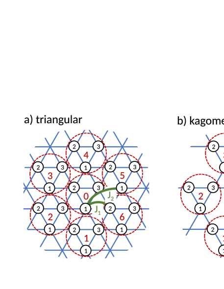
Figure 1: (a) Triangular and (B) kagome lattice represented as the (triangular) lattices of coupled basic triangles. Shown are also model exchange couplings on both lattices.

As shown in Fig. 1 the model Eq. (2) on both lattices can be represented as coupled basis triangles Subrahmanyam (1995); Mila (1998); Budnik and Auerbach (2004); Capponi et al. (2004) where we keep in the construction of the EM only four degenerate $S=1/2$ states (local energy $\epsilon_{0}=-3/4$), neglecting higher $S=3/2$ states (local $\epsilon_{1}=3/4$),

$$|\uparrow\pm\rangle = \frac{1}{\sqrt{3}}[|\downarrow\uparrow\uparrow\rangle+\mathrm{e}^{\pm i\phi}|\uparrow\downarrow\uparrow\rangle+\mathrm{e}^{\mp i\phi}|\uparrow\uparrow\downarrow\rangle],$$

$$|\downarrow\pm\rangle = \frac{1}{\sqrt{3}}[|\uparrow\downarrow\downarrow\rangle+\mathrm{e}^{\mp i\phi}|\downarrow\uparrow\downarrow\rangle+\mathrm{e}^{\mp i\phi}|\downarrow\downarrow\uparrow\rangle],$$ (3)

where $\phi=2\pi/3$, $\uparrow,\downarrow$ are (new) spin states and $\pm$ refer to local chirality. One can rewrite Eq.(2) into the new basis acting between nn triangles $\langle i,j\rangle$. The derivation is straightforward taking care that the matrix elements of the original model. Eq. (2), within the new basis, Eq. (3), are exactly reproduced with new operators. We follow the procedure through intermediate (single triangle) orbital spin operators (see Fig. 1),

$$S_{(0,+,-)}=S_{1}+(1,\omega,\omega^{*})S_{2}+(1,\omega^{*},\omega)S_{3},$$ (4)

with $\omega=\mathrm{e}^{i\phi}$. Operators in Eq. (4) have only few nonzero matrix elements within the new basis, Eq. (3), e.g.,

$$\langle\uparrow+|S_{0}^{z}|\uparrow+\rangle=-\langle\downarrow+|S_{0}^{z}|\downarrow+\rangle=\frac{1}{2},$$

$$\langle\downarrow+|S_{-}^{z}|\downarrow-\rangle=-\langle\uparrow+|S_{-}^{z}|\downarrow+\rangle=1,$$

$$\langle\uparrow+|S_{0}^{+}|\downarrow+\rangle=\leavevmode\nobreak\ \leavevmode\nobreak\ \langle\uparrow-|S_{0}^{+}|\downarrow-\rangle=-1,$$

$$\langle\uparrow-|S_{+}^{+}|\downarrow+\rangle=\leavevmode\nobreak\ \leavevmode\nobreak\ \langle\downarrow+|S_{-}^{-}|\uparrow-\rangle=2.$$ (5)

Such operators can be fully represented in terms of standard local $s=1/2$ spin operators ${\bf s}$, and pseudospin (chirality) operators ${\bf\tau}$(again $\tau=1/2$),

$$S^{z}_{0}=s^{z},\quad S^{\pm}_{0}=-s^{\pm},$$

$$S^{z}_{\pm}=-2s^{z}\tau^{\mp},\quad S^{\pm}_{+}=2s^{\pm}\tau^{-},\quad S^{\pm}_{-}=2s^{\pm}\tau^{+},$$ (6)

Since the original Hamiltonian, Eq. (2), acts only between two sites on the new reduced (triangular) lattice, the effective model (EM), subtracting local $\epsilon_{0}$, can be fully represented for both lattices (as shown by an example further on) in terms of ${\bf s}_{i}$ and ${\bf\tau}_{i}$ operators, introduced in Eq. (5),

$$\tilde{H} = \frac{1}{2}\sum_{i,d}{\bf s}_{i}\cdot{\bf s}_{j}(D+{\cal H}^{d}_{ij}),$$ (7)

$${\cal H}^{d}_{ij} = F_{d}\tau^{+}_{i}\tau^{-}_{j}+P_{d}\tau^{+}_{i}+Q_{d}\tau^{+}_{j}+T_{d}\tau^{+}_{i}\tau^{+}_{j}+\mathrm{H.c},$$

where directions $d=1$–$6$ and $j=i+d$ run over all nn sites of site $i$, and the new lattice is again TL. We note that Eq. (7) corresponds to the one studied before for simplest KL Subrahmanyam (1995); Mila (1998); Budnik and Auerbach (2004), but it is valid also for TL Subrahmanyam (1995) and nnn $J_{2}$. It is remarkable that the spin part remains $SU(2)$ invariant whereas the chirality part is not, i.e., it is of the XY form.

It should be pointed out that EM, Eq. (7), is not based on a perturbation expansion assuming weak coupling between triangles, although in the latter case it offers a full description of low-lying states and can be further treated analytically in (rather artificial) strong breathing limit $|\tilde{H}|\ll|E_{0}|$ Subrahmanyam (1995); Mila (1998). As for several other applications of reduced effective models (prominent example being the $t$-$J$ model as reduced/projected Hubbard model), one expects that low-$T$ physics is (at least qualitatively) well captured by the EM.

II.1 Triangular lattice

For the considered TL and KL we further present the actual parameters of the EM, Eq. (7). The derivation is straightforward using the representation Eqs. (4) and (6). As an example we present the $J_{1}$-term interaction in Eq. (2) between (new) sites $0$ and $1$ (see Fig. 1a),

$$\leavevmode\nobreak\ \leavevmode\nobreak\ \leavevmode\nobreak\ \leavevmode\nobreak\ \tilde{H}^{1}_{01}/J_{1}={\bf S}_{01}\cdot({\bf S}_{12}+{\bf S}_{13})=$$

$$=\frac{1}{9}(S_{00}^{z}+S^{z}_{0+}+S^{z}_{0-})(2S^{z}_{10}-S^{z}_{1+}-S^{z}_{1-})+$$

$$+\frac{1}{18}[(S_{00}^{+}+S^{+}_{0+}+S^{+}_{0-})(2S^{-}_{10}-S^{-}_{1+}-S^{-}_{1-})+\mathrm{H.c.}]=$$

$$=-\frac{4}{9}{\bf s}_{0}\cdot{\bf s}_{1}(\tau^{-}_{0}+\tau^{+}_{0}-\frac{1}{2})(\tau^{-}_{1}+\tau^{+}_{1}+1).$$ (8)

Deriving in the same manner also other $\tilde{H}^{d}$ terms, including now also $J_{2}$ term (which are even simpler in TL), we can identify the parameters (with $J_{1}=1$) in the EM, Eq.(7),

$$D=\frac{2}{9}+\frac{1}{3}J_{2},\qquad F=-\frac{4}{9}+\frac{4}{3}J_{2},$$ (9)

and further terms depending explicitly on direction $d$,

$$P_{1} = -\frac{4}{9},\quad P_{2}=\frac{2}{9}\omega^{*},\quad P_{3}=-\frac{4}{9}\omega,$$

$$P_{4} = \frac{2}{9},\quad P_{5}=-\frac{4}{9}\omega^{*},\quad P_{6}=\frac{2}{9}\omega,$$

$$T_{1} = -\frac{4}{9},\quad T_{2}=-\frac{4}{9}\omega,\quad T_{3}=-\frac{4}{9}\omega^{*}$$ (10)

with $T_{d+3}=T_{d}$ and $Q_{d}=P_{d+3}$. It is worth noticing, that $J_{2}$ does not enter in terms $P_{d},Q_{d},T_{d}$. It can be also directly verified, that for the latter couplings, the average over all nn bonds vanish, i.e.,

$$\bar{P}=\frac{1}{6}\sum_{d}P_{d}=0,\qquad\bar{Q}=\bar{T}=0,$$ (11)

indicating possible minor importance of these terms. This is, however, only partially true since such terms also play a role of distributing the increase of entropy $s(T)$ to a wider $T$ interval.

Eqs. (7),(9) yield also some basic insight into the HM model on TL, as well the similarity between models on TL and KL. While $\chi_{0}(T)$ is governed entirely by ${\bf s}$ operators, low-$T$ entropy $s(T)$ (and specific heat $C_{V}(T)$) involves also chirality ${\bf\tau}$ fluctuations. In TL at $J_{2}=0$ $\tau$ coupling is ferromagnetic and favors spiral $120^{0}$ LRO. $\tau$ fluctuations are enhanced via $J_{2}>0$ reducing $F$ and finally $F\to 0$ on approaching $J_{2}\sim 0.3$. Still, before such large $J_{2}$ is reached $P_{d},Q_{d},T_{d}$ terms become relevant and stabilize SL at $J_{2}\sim 0.1$ Kaneko et al. (2014); Watanabe et al. (2014); Zhu and White (2015); Hu et al. (2015); Iqbal et al. (2016). It should be stressed that in TL a standard magnetic LRO requires LRO ordering of both ${\bf s}$ and ${\bf\tau}$ operators.

II.2 Kagome lattice.

In analogy to the TL example, Eq. (8), we derive also the corresponding terms for the case of KL. Without loosing the generality we can include here also the third-neighbor exchange term $J_{3}$, see Fig. 1b, which also couples only neighboring triangles. Then $D$ and $F_{d}$ couplings are given by

$$D=\frac{1}{9}+\frac{2}{9}J_{2}+\frac{2}{9}J_{3},\qquad F_{1}=\frac{4}{9}\omega+\frac{8}{9}\omega^{*}J_{2}+\frac{4}{9}J_{3},$$ (12)

while $F_{d+1}=F_{d}^{*}$. In contrast to TL, in KL at $J_{2}=0$ the $F_{d}$ coupling is complex and alternating, with a nonzero average, being real and negative, i.e. $\bar{F}=(1/6)\sum_{d}F_{d}<0$. Moreover, $|\mathrm{Im}F_{d}|<|\mathrm{Re}F_{d}|$, indicates the absence of LRO. Here, $J_{2}>0$ reduces $|\mathrm{Im}F_{d}|$ and on approaching $J_{2}\sim 0.5$ one reaches real $F_{d}<0$ connecting KL model to TL at $J_{2}=0$ and related LRO, as observed in numerical studies Kolley et al. (2015).

Further terms are given by

$$P_{1} = -\frac{2}{9}+\frac{2}{9}\omega^{*}J_{2}-\frac{2}{9}\omega J_{3},\quad P_{2}=-\frac{2}{9}\omega+\frac{2}{9}\omega^{*}J_{2}-\frac{2}{9}J_{3},$$

$$P_{3} = -\frac{2}{9}\omega+\frac{2}{9}J_{2}-\frac{2}{9}\omega^{*}J_{3},\quad P_{4}=-\frac{2}{9}\omega^{*}+\frac{2}{9}J_{2}-\frac{2}{9}\omega J_{3},$$

$$P_{5} = -\frac{2}{9}\omega^{*}+\frac{2}{9}\omega J_{2}-\frac{2}{9}J_{3},\quad P_{6}=-\frac{2}{9}+\frac{2}{9}\omega J_{2}-\frac{2}{9}\omega^{*}J_{3},$$

with $Q_{d}=P_{d+3}$ and

$$T_{1} = \frac{4}{9}\omega^{*}-\frac{4}{9}\omega^{*}J_{2}+\frac{4}{9}J_{3},\quad T_{2}=\frac{4}{9}-\frac{4}{9}J_{2}+\frac{4}{9}J_{3},$$

$$T_{3} = \frac{4}{9}\omega-\frac{4}{9}\omega J_{2}+\frac{4}{9}J_{3},\qquad T_{d+3}=T_{d}.$$ (14)

Again, terms which do not conserve $\tau^{z}_{tot}$ have the property $\bar{P}=\bar{Q}=\bar{T}=0$.

III Numerical method

In the evaluation of thermodynamical quantities we use the FTLM Jaklič and Prelovšek (1994, 2000); Prelovšek and Bonča (2013), which is based on the Lanczos exact-diagonalization (ED) method Lanczos (1950), whereby the Lanczos-basis states are used to evaluate the normalized thermodynamic sum

$$Z(T)=\mathrm{Tr}\exp[-(H-E_{0})/T],$$ (15)

(where $E_{0}$ is the ground state energy of a system). The FTLM is particularly convenient to apply for the calculation of the conserved quantities , i.e., operators $A$ commuting with the Hamiltonian $[H,A]=0$. In this way we evaluate $Z$, the thermal average energy $\Delta E=\langle H-E_{0}\rangle$ and magnetization $M=\langle s^{z}_{tot}\rangle$. From these quantities we evaluate the thermodynamic observables of interest, i.e. uniform susceptibility $\chi_{0}(T)$ and entropy density $s(T)$,

$$\chi_{0}=\frac{M^{2}}{NT},\qquad s=\frac{T\ln Z+\Delta E}{NT},$$ (16)

where $N$ is the number of sites in the original lattice.

We note that for above conserved operators $A$ there is no need to store Lanczos wavefunctions, so the requirements are essentially that of the g.s. Lanczos ED method, except that we need the summation over all symmetry sectors and a modest sampling $N_{s}<10$ over initial wavefunctions is helpful. To reduce the Hilbert space of basis states $N_{st}$ we take into account symmetries, in particular the translation symmetry (restricting subspaces to separate wavevectors $q$) and $s^{z}_{tot}$ while the EM, Eq. (7), does not conserve $\tau^{z}_{tot}$. In such a framework in the present study we are restricted to systems with $N_{st}<5\cdot 10^{6}$ symmetry-reduced basis states, which means EM with up to $N=42$ sites. The same system size would require in the full HM $N_{st}\sim 10^{10}$ basis states.

An effective criterion for the macroscopic relevance of FTLM results is $Z(T)\gg 1$ (at least for system where gapless excitations are expected), which in practice leads to a criterion $Z>Z^{*}=Z(T_{fs})\gg 1$ determining the finite-size temperature $T_{fs}$. Taking $Z^{*}\sim 20$ implies (for $N=42$) also the threshold entropy density $s(T_{fs})\sim 0.07$, independent of the model. It is then evident that $T_{fs}$ depends crucially on the model, so that large $s(T)$ works in favor of using FTLM for frustrated and SL systems. Here we do not present the finite-size analysis of FTLM results within EM, but they are quite analogous to previous application of the method to HM on KL Schnack et al. (2018) where similar low $T_{fs}$ was established (but much higher $T_{fs}$ ) in unfrustrated lattices and models Jaklič and Prelovšek (2000). Moreover, in the case of models with a sizable gap, e.g. $\Delta>T_{fs}$ the results of FTLM can remain correct even down to $T\to 0$. Jaklič and Prelovšek (2000)

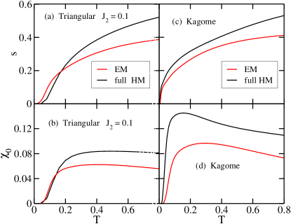
Figure 2: Results for the effective model (EM) for the triangular lattice, compared with the full HM. All results for are for $N=30$ sites Prelovšek and Kokalj (2018): a) for entropy density $s(T)$ and b) uniform susceptibility $\chi_{0}(T)$. c) and d) same quantities for the kagome lattice, compared to full HM, all on $N=42$ sites Schnack et al. (2018).

IV Entropy and uniform susceptibility

Let us first benchmark results within the EM with the existing results for the full HM on TL and KL. In Figs. 2a,b we present $s(T)$ and $\chi_{0}(T)$, respectively, as obtained on TL for $J_{2}=0.1$ on $N=30$ via FTLM on EM, compared with the full HM of the same size Prelovšek and Kokalj (2018). The qualitative behavior of both quantities within EM is quite similar at low $T$ to the full HM, in particular for $s(T)$, although EM evidently misses part of $s(T)$ with increasing $T$ due to reduced basis space. More pronounced is quantitative (but not qualitative) discrepancy in $\chi_{0}(T)$ which can be attributed to missing higher spin states in EM. Still, the peak in $\chi_{0}(T)$ and related spin (triplet) gap $\Delta_{t}>0$ at low $T$) are reproduced well within EM. Similar conclusions emerge from Figs. 2c,d where corresponding results are compared for the KL, where full-HM results for $s(T)$ and $\chi_{0}(T)$ are taken from study on $N=42$ sites Schnack et al. (2018). Here, EM clearly reproduces reasonably not only triplet gap $\Delta_{t}\sim 0.1$ but also singlet excitations dominating $s(T\to 0)$, while apparently EM underestimates the value of $\chi_{0}(T)$.

After testing with the full model, we present in Figs. 3 and 4 EM results for $s(T)$ and $\chi_{0}(T)$ for both lattices as they vary with $J_{2}>0$. In Fig. 3a,b we follow the behavior on TL for different $J_{2}=0,0.1,0.15$. From the inflection (vanishing second derivative) point of $s(T)$ defining singlet temperature $T=T_{s}$ one can speculate on the coherence scale (in the case of LRO) or possible (singlet) excitation gap $\Delta_{s}\lesssim T_{s}$ (in the case of SL), at least provided that $T_{s}>T_{fs}$. Although the influence of $J_{2}>0$ does not appear large, it still introduces a qualitative difference. From this perspective $s(T)$ within TL EM at $J_{2}=0$ reveals higher effective $T_{s}$ being consistent with $s(T<T_{s})\propto T^{2}$ and a spiral LRO at $T=0$. Still, we get in this case $T_{s}\sim T_{fs}$ within EM, so we can hardly make stronger conclusions.

On the other hand, for TL and $J_{2}=0.1,0.15$ where the SL can be expected Kaneko et al. (2014); Iqbal et al. (2016); Gong et al. (2017) the EM reveals smaller $T_{s}\sim 0.05$ which is the signature of the singlet gap (which could still be finite-size dependent). More important, results confirm large residual entropy $s(T)\sim 0.1=0.14s_{max}$ even at $T\sim 0.1$. This is in contrast with $\chi_{0}(T)$ in Fig. 3b which reveal $T$-variation weakly dependent on $J_{2}$. While for $J_{2}=0$ the drop at $\chi_{0}(T<T_{t})$ is the signature of the finite-size spin gap (where due to magnetic LRO $\chi_{0}^{0}=\chi_{0}(T\to 0)>0$ is expected), $J_{2}=0.1,0.15$ examples are different since vanishing $\chi_{0}^{0}$ could indicate the spin triplet gap $\Delta_{t}>0.1$ beyond the finite-size effects, i.e. $T_{t}\sim 0.1>T_{fs}$.

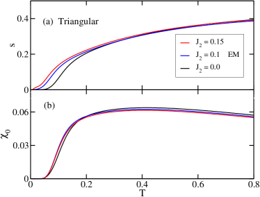
Figure 3: Results within EM on triangular lattice for different $J_{2}=0,0.1,0.15$; a) for $s(T)$, and b) $\chi_{0}(T)$.

In Figs. 4a,b we present the same quantities for the case of KL, now for $J_{2}=0,0.2,0.4$. The effect of $J_{2}>0$ is opposite, since it is expected to recover the LRO at $J_{2}\sim 0.4$ Kolley et al. (2015), with $120^{0}$ spin orientation analogous to $J_{2}=0$ TL. The largest low-$T$ entropy $s(T)$ is found for KL with $J_{2}=0$. Moreover, EM here yields a quantitive agreement with the full HM Schnack et al. (2018), revealing large remanent $s(T)$ due to singlet (chirality) excitations down to $T\sim 0.01$ Läuchli et al. (2019). The evident effect of $J_{2}>0$ is to reduce $s(T)$ and finally leading $s(T)\propto T^{2}$ at large $J_{2}\sim 0.4$ which should be a regime of magnetic LRO Kolley et al. (2015). Again, at $J_{2}=0$ in contrast to entropy $\chi_{0}(T)$ has well pronounced downturn at $T\sim 0.1$ consistent with the triplet gap $\Delta_{t}\sim 0.1$ found in most other numerical studies Sindzingre et al. (2000); Misguich and Sindzingre (2007); Bernu and Lhuillier (2015); Schnack et al. (2018); Läuchli et al. (2019). Introducing $J_{2}>0$ does not change $\chi_{0}(T)$ qualitatively.

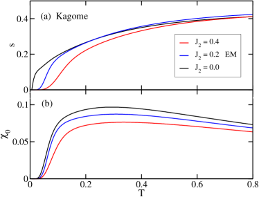
Figure 4: Results within EM on kagome lattice for different $J_{2}=0,0.2,0.4$; a) for $s(T)$, and b) $\chi_{0}(T)$.

V Wilson ratio: results

To calculate $R(T)$, Eq. (1), let us first use available results for the full HM for TL Prelovšek and Kokalj (2018) and KL Schnack et al. (2018), comparing in Fig. 5 also the result for unfrustrated HM on a square lattice Prelovšek and Kokalj (2018). Here, we take into account data for $T>T_{fs}$, acknowledging that $T_{fs}$ are quite different (taking $s(T_{fs})\sim 0.1$ as criterion) for these systems, representative also for the degree of frustration. Fig. 5 already confirms different scenarios for $R(T)$. In HM on a simple square lattice, starting from high-$T$ limit $R(T)$ reaches minimum at $T^{*}\sim 0.7$ and then increases, which is consistent with $R(T\to 0)\to\infty$ for a 2D system with $T=0$ magnetic LRO. The same behavior appears for TL at $J_{2}=0$ with a shallow minimum shifted to $T^{*}\sim 0.3$. In contrast, results for KL as well as for TL with $J_{2}=0.1$ do not reveal such increase, at least not for $T>T_{fs}$, and they are more consistent with the interpretation that $R(T\to 0)\to 0$.

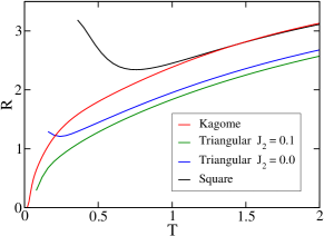
Figure 5: Wilson ratio $R(T)$, evaluated from $s(T)$ and $\chi_{0}(T)$ for full HM on square lattice, triangular lattice with $J_{2}=0,0.1$ Prelovšek and Kokalj (2018), and kagome lattice Schnack et al. (2018). Results are presented for $T>T_{fs}$.

Finally, results for $R(T)$ within EM are shown in Fig. 6a,b as they follow from Figs. 3 and 4 for different $J_{2}\geq 0$. We recognize that EM qualitatively reproduce numerical data within the full HM on Fig. 5. Although for $J_{2}=0$ TL results in Fig. 6a fail to reveal clearly the minimum down to $T_{fs}\sim 0.1$, there is still a marked difference to the SL regime $J_{2}=0.1,0.15$ where EM confirms $R_{0}\ll 1$. Results within EM for KL, as shown in Fig. 6b, are even better demonstration for vanishing $R_{0}$. Here, for $J_{2}=0$ EM yields quite similar $R(T)$, decreasing and tending towards $R_{0}\sim 0$. On the other hand, the effect of finite $J_{2}>0$ is well visible and leads towards magnetic LRO with $R_{0}\to\infty$ for $J_{2}=0.4$.

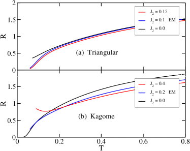
Figure 6: $R(T)$, evaluated within EM for: a) TL with $J_{2}=0,0.1,0.15$, and b) KL for $J_{2}=0,0.2,0.4$.

VI Conclusions

The main message (apparently not stressed in previous published studies of the SL models) of presented results for the thermodynamic quantities: the entropy $s(T)$, susceptibility $\chi_{0}(T)$, and in particular the Wilson ratio $R(T)$, behave similarity in the extended $J_{1}$-$J_{2}$ Heisenberg model on TL and KL in their presumed SL regimes. Moreover, results on both lattices follow quite analogous development by varying the nnn exchange $J_{2}>0$, whereby the effect is evidently opposite between TL and KL, regarding the magnetic LRO and SL phases Kolley et al. (2015).

While above similarities can be extracted already from full-model results obtained via FTLM Schnack et al. (2018); Prelovšek and Kokalj (2018), the introduction of reduced effective model appears crucial for the understanding and useful analytical insight. Apart from offering some numerical advantages of reduced Hilbert space of basis states, essential for ED methods, EM clearly puts into display two (separate) degrees of freedom: a) the effective spin $s=1/2$ degrees ${\bf s}_{i}$, determining $\chi_{0}(T)$, but as well the dynamical quantities, as e.g. the dynamical spin structure factor $S({\bf q},\omega)$ not discussed here Prelovšek and Kokalj (2018), b) chirality pseudospin degrees ${\bf\tau}_{i}$ which do not contribute to $\chi_{0}(T)$, but enter the entropy $s(T)$ and related specific heat. From the EM and its dependence on $J_{2}$ it is also quite evident where to expect large fluctuations of ${\bf\tau}_{i}$ and consequently SL regime, which is not very apparent within the full HM. As the EM is based on the direct reduction/projection of the basis (and not on perturbation expansion) of the original HM, it is expected that the correspondence is qualitative and not fully quantitative. In any case, the EM is also by itself a valuable and highly nontrivial model, and could serve as such to understand better the onset and properties of SL.

The essential common feature of SL regimes in HM on both lattices is a pronounced remanent $s(T)>0$ at $T\ll J_{1}$, which within the EM has the origin in dominant low-energy chiral fluctuations, well below the effective spin triplet gap $\Delta_{t}$ which is revealed by the drop of $\chi_{0}(T)$. As a consequence we observe the vanishing of the Wilson ratio $R_{0}=R(T\to 0)\to 0$, which seems to be quite generic feature of 2D SL models Prelovšek et al. . Clearly, due to finite-size restrictions we could hardly distinguish a spin-gapped system from scenarios with more delicate gap structure which could also lead to renormalized $R_{0}\ll 1$. Moreover, it is even harder to decide beyond finite-size effects whether singlets excitations are gapless or with finite singlet gap $\Delta_{s}>0$, which should be in any case very small $\Delta_{s}\ll J$ and from results $R(T\to 0)\to 0$ have to be evidently smaller than a triplet one, i.e. $\Delta_{s}<\Delta_{t}$. From our finite-size results it is also hard to exclude the scenario of valence-bond ordered ground state (with broken translational symmetry), although we do not see an indication for that and vanishing $R_{0}$, it is also not easily compatible with the latter either.

Quantities discussed above are measurable in real materials and have been indeed discussed for some of them. There are evident experimental difficulties, i.e., $\chi_{0}(T)$ can have significant impurity contributions while $s(T)$ may be masked by phonon contribution at $T>0$. The essential hallmark for material candidates for the presented SL scenario should be a substantial entropy $s(T)$ persisting well below $T\ll J_{1}$. There are indeed several studies of $s(T)$ reported for different SL candidates (with some of them revealing transitions to magnetic LRO at very low $T$), e.g., for KL systems volborthite Hiroi et al. (2001), YCu₃(OH)₆Cl₃ Zorko et al. (2019); Arh et al. , and recent TL systems 1T-TaS₂ Kratochvilova et al. (2017) and Co-based SL materials Zhong et al. (2019). While existing experimental results on SL materials do not seem to indicate vanishing (or very small) $R_{0}$, it might also happen that the (above) considered SL models are not fully capturing the low-$T$ physics. In particular, there could be important role played by additional terms, e.g., the Dzaloshinski-Moriya interaction Cépas et al. (2008); Rousochatzakis et al. (2009); Arh et al. and/or 3D coupling, which can reduce $s(T)$ or even induce magnetic LRO at $T\to 0$.