Abstract

We study inflation in Weyl gravity. The original Weyl quadratic gravity, based on Weyl conformal geometry, is a theory invariant under the Weyl symmetry of gauged scale transformations. In this theory the Planck scale ($M$) emerges as the scale where this symmetry is broken spontaneously by a geometric Stueckelberg mechanism, to Einstein-Proca action for the Weyl “photon” (of mass near $M$). With this action as a “low energy” broken phase of Weyl gravity, century-old criticisms of the latter (due to non-metricity) are avoided. In this context, inflation with field values above $M$ is natural, since this is just a phase transition scale from Weyl gravity (geometry) to Einstein gravity (Riemannian geometry), where the massive Weyl photon decouples. We show that inflation in Weyl gravity coupled to a scalar field has results close to those in Starobinsky model (recovered for vanishing non-minimal coupling), with a mildly smaller tensor-to-scalar ratio ($r$). Weyl gravity predicts a specific, narrow range $0.00257\leq r\leq 0.00303$, for a spectral index $n_{s}$ within experimental bounds at $68\%$CL and e-folds number $N\!=\!60$. This range of values will soon be reached by CMB experiments and provides a test of Weyl gravity. Unlike in the Starobinsky model, the prediction for $(r,n_{s})$ is not affected by unknown higher dimensional curvature operators (suppressed by some large mass scale) since these are forbidden by the Weyl gauge symmetry.

1 Motivation

There is a renewed interest in studying scale invariant models for physics beyond Standard Model (SM) and cosmology. This symmetry may also be present at the quantum level [1, 2, 3, 4]. All scales (including the scale of “new physics” beyond SM) are generated spontaneously by field vev’s and this symmetry may even preserve a classical hierarchy of scales [2, 3, 4, 5, 6, 7, 8, 9, 10, 11]. In cosmology there are global [12, 13, 14, 15, 18, 19, 22, 23, 27, 28, 17, 16, 21, 20, 24, 25, 26] or local [30, 35, 29, 33, 34, 36, 37, 38, 39, 40, 32, 31] scale invariant alternatives to gravity with spontaneous breaking that generates the Planck scale by a non-minimal coupling.

In this paper we study inflation in a theory with gauged scale invariance. The theory considered is the original Weyl gravity [41, 42, 43], based on Weyl conformal geometry [44]. This symmetry is also referred to as Weyl gauge symmetry and its associated gauge boson is called hereafter Weyl “photon”. This theory has no fundamental scale (Planck scale, etc), forbidden by its symmetry. Weyl action is [41, 42, 43]

$$L_{0}=\sqrt{g}\,\Big{\{}\frac{\xi_{0}}{4!}\,\tilde{R}^{2}-\frac{1}{4q^{2}}\,F_{\mu\nu}^{2}\Big{\}}$$ (1)

Each term is Weyl gauge invariant (see later, eq.(6)); $\tilde{R}$ is the scalar curvature of Weyl geometry; $F_{\mu\nu}$ is the field strength of the Weyl “photon” $\omega_{\mu}$, with coupling $q$. In addition to $L_{0}$, one can also include an independent Weyl-tensor-squared term of Weyl geometry, allowed by the symmetry and considered later. A topological Gauss-Bonnet term of Weyl geometry may be present too, not relevant here. However, higher dimensional operators ($\tilde{R}^{4}$, etc) cannot be present in $L_{0}$ since there is no scale to suppress them.

As recently shown in [38, 39] scale dependence in Weyl gravity (1) emerges spontaneously after a geometric version of Stueckelberg breaking mechanism [46] of Weyl gauge symmetry: the dilaton, which is the Goldstone mode of this symmetry (and spin 0 mode propagated by $\tilde{R}^{2}$) is absorbed by the Weyl “photon” which thus becomes massive. Denoting by $R$ the Ricci scalar of Riemannian geometry, action (1) becomes [38, 39]:

$$L_{0}=\sqrt{g}\,\Big{\{}-\frac{1}{2}M^{2}\,R-\frac{3\,M^{2}}{2\,\xi_{0}}-\frac{1}{4}F_{\mu\nu}^{2}+\frac{3}{4}q^{2}M^{2}\omega_{\mu}\omega^{\mu}\Big{\}}.$$ (2)

The Planck scale $M$ is fixed by the dilaton vev and the Weyl “photon” acquired a mass $\sim qM$ near the Planck scale (for $q$ not too small). Therefore the Einstein-Proca action (2) is just a “low-energy” broken phase of Weyl gravity: it is obtained after “gauge fixing” the Weyl gauge symmetry. This involves fixing the dilaton vev which in a FRW universe is a dynamical effect [47]. Given its equivalence to action (2), Weyl action (1) avoids long-held criticisms since Einstein [42] related to non-metricity effects due to $\omega_{\mu}$, e.g. the changing of atomic lines spacing, that can be safely ignored since $\omega_{\mu}$ decouples near Planck scale $M$.

Having Einstein gravity as a “low-energy” limit of Weyl action motivates us to study inflation in Weyl gravity. Moreover, the presence of $\tilde{R}^{2}$ in (1) points to similarities to successful Starobinsky inflation [48]. And since Planck scale is just a phase transition scale, field values above $M$ are natural in Weyl gravity. This is relevant for inflation where such values are common but harder to accept in models where Planck scale is the physical cutoff.

2 Weyl gravity and inflation

To study Weyl inflation we review briefly the action of Weyl gravity coupled to a scalar field $\phi_{1}$, see [38, 39] for a detailed analysis. The Lagrangian is

$$L=\sqrt{g}\,\Big{[}\,\frac{\xi_{0}}{4!}\,{\tilde{R}}^{2}-\frac{1}{4\,q^{2}}\,F_{\mu\nu}^{2}\Big{]}-\frac{\sqrt{g}}{12}\,\xi_{1}\phi_{1}^{2}\,{\tilde{R}}+\sqrt{g}\,\Big{[}\frac{1}{2}\,g^{\mu\nu}\,\tilde{D}_{\mu}\phi_{1}\tilde{D}_{\nu}\phi_{1}-\frac{\lambda_{1}}{4!}\phi_{1}^{4}\Big{]},$$ (3)

with couplings $\xi_{0}$, $\xi_{1}$, $\lambda_{1}$; $F_{\mu\nu}=\partial_{\mu}\omega_{\nu}-\partial_{\nu}\omega_{\mu}$ (no torsion). $\tilde{D}_{\mu}$ is a Weyl-covariant derivative

$$\tilde{D}_{\mu}\phi_{1} = (\partial_{\mu}-1/2\,\omega_{\mu})\,\phi_{1},$$ (4)

$${\tilde{R}} = R-3\,D_{\mu}\omega^{\mu}-\frac{3}{2}\,\omega^{\mu}\omega_{\mu},$$ (5)

with the scalar curvature of Weyl geometry ($\tilde{R}$) related to its Riemannian counterpart ($R$) as above. Lagrangian (3) is invariant under a Weyl gauge transformation $\Omega(x)$:

$$\hat{g}_{\mu\nu}=\Omega\,g_{\mu\nu},\qquad\hat{\phi}_{1}=\frac{1}{\sqrt{\Omega}}\,\phi_{1},\qquad\hat{\omega}_{\mu}=\omega_{\mu}-\,\partial_{\mu}\ln\Omega,\quad\Rightarrow\quad\hat{\tilde{R}}=\frac{1}{\Omega}\,{\tilde{R}}.$$ (6)

where $\omega_{\mu}$ is the Weyl gauge field. We also have $\sqrt{\hat{g}}\!=\!\Omega^{2}\!\sqrt{g}$,  $g\!\equiv\!|\det g_{\mu\nu}|$, $\hat{g}^{\mu\nu}=\Omega^{-1}\,g^{\mu\nu}$, and metric $(+,-,-,-)$. Our conventions are those of [50].

Unlike the Riemannian scalar curvature ($R$), ${\tilde{R}}$ is computed from a Weyl connection invariant under (6) and it transforms covariantly, due to the inverse metric entering its definition. With this observation, one sees the advantage of Weyl formulation (i.e. using ${\tilde{R}}$) instead of the Riemannian language (using $R$) and why $L$ is invariant under (6).

One “linearises” (3) by using an auxiliary field $\phi_{0}$ to replace ${\tilde{R}}^{2}\!\rightarrow\!-2\phi_{0}^{2}{\tilde{R}}-\phi_{0}^{4}$ and to obtain a classically equivalent action. Indeed the equation of motion for $\phi_{0}$ has solution $\phi_{0}^{2}=-{\tilde{R}}$, which when used back in the action recovers (3). Given this, $\phi_{0}$ transforms as any other scalar field. Therefore

$$L=\sqrt{g}\,\Big{[}-\frac{1}{4\,q^{2}}F_{\mu\nu}^{2}-\frac{1}{12}(\xi_{0}\,\phi_{0}^{2}+\xi_{1}\phi_{1}^{2})\,{\tilde{R}}+\frac{1}{2}\,g^{\mu\nu}\,\tilde{D}_{\mu}\phi_{1}\tilde{D}_{\nu}\phi_{1}-\frac{1}{4!}(\lambda_{1}\phi_{1}^{4}+\xi_{0}\phi_{0}^{4})\Big{]},$$ (7)

Next, we must fix the gauge which we do by a particular Weyl “gauge-fixing” transformation (6) of $\Omega=\rho^{2}/M^{2}$ and $\rho=(1/6)(\xi_{1}\phi_{1}^{2}+\xi_{0}\phi_{0}^{2})$ with $M$ some scale (see later). We find

$$L=\sqrt{\hat{g}}\,\Big{[}-\frac{1}{2}M^{2}\,\hat{R}+\frac{3}{4}\,M^{2}\,\hat{\omega}_{\mu}\hat{\omega}^{\mu}-\frac{1}{4q^{2}}\hat{F}_{\mu\nu}^{2}+\frac{\hat{g}^{\mu\nu}}{2}\hat{\tilde{D}}_{\mu}\hat{\phi}_{1}\hat{\tilde{D}}_{\nu}\hat{\phi}_{1}-\hat{V}\Big{]},$$ (8)

with $\hat{R}$ the Riemannian scalar curvature and

$$\hat{V}=\frac{3M^{4}}{2\,\xi_{0}}\Big{[}1-\frac{\xi_{1}\hat{\phi}_{1}^{2}}{6\,M^{2}}\Big{]}^{2}+\frac{\lambda_{1}}{4!}\,\hat{\phi}_{1}^{4}.$$ (9)

Therefore, as detailed in [38, 39], the Weyl “photon” has become massive via a Stueckelberg mechanism by “absorbing” the field $\ln\rho\sim\ln\Omega$, eq.(6), of the radial direction in the field space $\phi_{0}$, $\phi_{1}$. This is the Goldstone (dilaton) mode since under (6) $\ln\rho$ has a shift symmetry $\ln\rho^{2}\rightarrow\ln\rho^{2}-\ln\Omega$. Weyl gauge symmetry is now spontaneously broken and Einstein gravity is recovered as a “low-energy” broken phase of Weyl gravity (this is consistent with the fact that Riemannian-based $R^{2}$-gravity is equivalent to Einstein gravity plus a massless mode [17] eaten here by the Weyl “photon”). The scale of breaking and the mass of Weyl “photon” is $\sim qM$, with $M$ identified with the Planck scale. $M$ is itself fixed by the vev of the radial direction which in a FRW universe is fixed dynamically [47] following a conserved current which drives the dilaton field to a constant value. The Planck scale and the mass of $\omega_{\mu}$ are thus determined by the dilaton vev. Fields values above $M$ are naturally allowed here since $M$ is just a phase transition scale in the theory.

The Weyl-covariant derivative acting on $\hat{\phi}_{1}$ in (8) is a remnant of the initial Weyl gauge symmetry, now broken; one would like to decouple $\partial_{\mu}\hat{\phi}_{1}$ from $\omega^{\mu}$ in order to study inflation; for a “standard” kinetic term for $\hat{\phi}_{1}$, a field redefinition is used

$$\hat{\omega}_{\mu}^{\prime}=\hat{w}_{\mu}-\partial_{\mu}\ln\cosh^{2}\frac{\sigma}{M\sqrt{6}},\qquad\hat{\phi}_{1}=M\sqrt{6}\,\sinh\Big{[}\frac{\sigma}{M\sqrt{6}}\Big{]}$$ (10)

to find

$$L=\sqrt{\hat{g}}\,\Big{\{}-\frac{1}{2}M^{2}\,\hat{R}+\frac{3}{4}M^{2}\cosh^{2}\Big{[}\frac{\sigma}{M\sqrt{6}}\Big{]}\,\hat{\omega}^{\prime}_{\mu}\hat{\omega}^{\prime\,\mu}-\frac{1}{4q^{2}}\hat{F}^{\prime\,2}_{\mu\nu}+\frac{\hat{g}^{\mu\nu}}{2}\partial_{\mu}\sigma\partial_{\nu}\sigma-V\Big{\}}.$$ (11)

Finally, one rescales above $\hat{\omega}_{\mu}^{\prime}\rightarrow q\hat{\omega}_{\mu}^{\prime}$, for a canonical gauge kinetic term. The potential is

$$V = V_{0}\,\,\Big{\{}\,\Big{[}1-\xi_{1}\sinh^{2}\frac{\sigma}{M\sqrt{6}}\Big{]}^{2}+\lambda_{1}\xi_{0}\,\sinh^{4}\frac{\sigma}{M\sqrt{6}}\Big{\}},\qquad V_{0}=\frac{3}{2}\,\frac{M^{4}}{\xi_{0}}.$$ (12)

$V$ encodes the effect of the initial presence of the Weyl “photon”. The potential has a minimum due to the non-minimal gravitational coupling $\xi_{1}>0$ and this is relevant for inflation; we assume $\sigma$ as the inflaton, with $V$ its potential.

3 Results

$V$ of (12) is largely controlled by $\xi_{1}$ and the combination $\lambda_{1}\xi_{0}$. Its minimum is at:

$$\frac{\sigma_{\text{min}}}{M\sqrt{6}}=\ln\Big{[}\gamma+\sqrt{1+\gamma^{2}}\Big{]},\quad\gamma=\Big{[}\frac{\xi_{1}}{\xi_{1}^{2}+\xi_{0}\,\lambda_{1}}\Big{]}^{1/2},\qquad V_{\text{min}}=\frac{3}{2}\,\frac{M^{4}\,\lambda_{1}}{\lambda_{1}\xi_{0}+\xi_{1}^{2}}.$$ (13)

The potential is shown in Figure 2 in function of the field $\sigma$, for different perturbative values of the non-minimal coupling $\xi_{1}$, with two fixed values of the product ($\xi_{0}\lambda_{1}$). Note that:

a) For $(\lambda_{1}\xi_{0})$ and $\xi_{1}$ small enough, $V$ is constant $V\approx V_{0}\sim 1/\xi_{0}$ and controlled by $\xi_{0}$.

b) Inflation begins in the region $V=V_{0}$ and lasts a number of e-folds that depends on the width of the flat region i.e. on the position of $\sigma_{\text{min}}\propto\gamma$. If $\lambda_{1}\xi_{0}\ll\xi_{1}^{2}$ then $\gamma\sim 1/\sqrt{\xi}_{1}$ so reducing $\xi_{1}$ will extend the flat region.

c) From the condition the initial energy be larger than at the end of inflation, $V_{0}\gg V_{\text{min}}$ then $\lambda_{1}\xi_{0}\ll\xi_{1}^{2}$ and also $V_{\text{min}}\approx 0$, as seen from eq.(12) and the second plot in Figure 2.

Constraints on the parametric space are found from the normalization of CMB anisotropy $V_{0}/(24\pi^{2}M^{4}\,\varepsilon_{*})=\kappa_{0},\quad\kappa_{0}\equiv 2.1\times 10^{-9}$ [51] where $\epsilon_{*}$ is the slow roll parameter. With tensor-to-scalar ratio $r=16\epsilon_{*}$ and $r<0.07$ [51] then $\xi_{0}=1/(\pi^{2}\,r\,\kappa_{0})\geq 6.89\times 10^{8}$. In conclusion we have the parametric constraints

$$\lambda_{1}\xi_{0}\ll\xi_{1}^{2},\qquad\xi_{0}\geq 6.89\times 10^{8}.$$ (14)

A large $\xi_{0}$ is always compensated by choosing an ultraweak value of $\lambda_{1}\!\ll\xi_{1}^{2}/\xi_{0}\sim 10^{-9}\xi_{1}^{2}$ so eq.(14) is respected for a chosen $\xi_{1}$ (note the coupling of $\tilde{R}^{2}$ is $1/\xi_{0}$ and is in the perturbative regime). We shall use these constraints to predict the spectral index $n_{s}$ and $r$.

The potential slow-roll parameters are

$$\qquad\quad\epsilon=\frac{M^{2}}{2}\,\Big{\{}\frac{V^{\prime}}{V}\Big{\}}^{2}=\frac{1}{3}\frac{\sinh^{2}(2\tilde{\sigma})\big{[}-\xi_{1}+(\lambda_{1}\xi_{0}+\xi_{1}^{2})\,\sinh^{2}\tilde{\sigma}\big{]}^{2}}{\big{[}1-2\,\xi_{1}\sinh^{2}\tilde{\sigma}+(\lambda\xi_{0}+\xi_{1}^{2})\,\sinh^{4}\tilde{\sigma}\big{]}^{2}},\quad\tilde{\sigma}\equiv\frac{\sigma}{M\sqrt{6}},$$ (15)

and

$$\eta=M^{2}\,\frac{V^{\prime\prime}}{V}=\frac{V_{0}}{3}\frac{(\lambda_{1}\xi_{0}+\xi_{1}^{2})\,\cosh(4\tilde{\sigma})-(2\,\xi_{1}+\lambda_{1}\xi_{0}+\xi_{1}^{2})\,\cosh(2\tilde{\sigma})}{1-2\xi_{1}\sinh^{2}\tilde{\sigma}+(\tilde{\lambda}+\xi_{1}^{2})\,\sinh^{4}\tilde{\sigma}}.$$ (16)

For $\lambda_{1}\xi_{0}\ll\xi_{1}^{2}$ and $\xi_{1}\ll 1$, slow roll conditions are met, $\epsilon,\eta\ll 1$, as seen from a numerical analysis. Further, the number $N$ of e-folds is

$$N = \frac{1}{M^{2}}\int_{\sigma_{e}}^{\sigma_{*}}d\sigma\,\frac{V(\sigma)}{V^{\prime}(\sigma)}={\cal N}(\sigma_{*})-{\cal N}(\sigma_{e})$$ (17)

with

$${\cal N}(\sigma)=c_{1}\,\ln\cosh\frac{\sigma}{M\sqrt{6}}+c_{2}\,\ln\Big{[}2\,(\lambda_{1}\xi_{0}+\xi_{1}^{2})\,\sinh^{2}\frac{\sigma}{M\sqrt{6}}-2\,\xi_{1}\Big{]}+c_{3}\ln\sinh\frac{\sigma}{M\sqrt{6}}$$ (18)

and

$$c_{1}=\frac{3}{2}\,\frac{\lambda_{1}\xi_{0}+(1+\xi_{1})^{2}}{\xi_{1}+\lambda_{1}\xi_{0}+\xi_{1}^{2}},\quad c_{2}=\frac{3\,\lambda_{1}\xi_{0}}{4\,\xi_{1}\,(\xi_{1}+\lambda_{1}\xi_{0}+\xi_{1}^{2})},\quad c_{3}=\frac{3}{-2\,\xi_{1}}.$$ (19)

Above $\sigma=\sigma_{*}$ is the value at the horizon exit. Inflation ends at $\sigma=\sigma_{e}$ found from $\epsilon=1$.

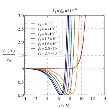
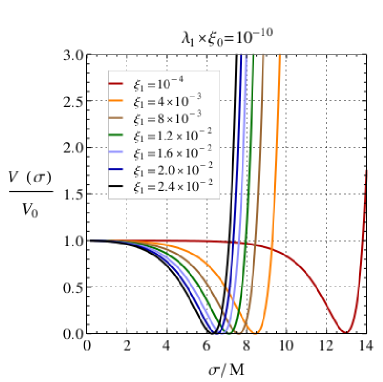
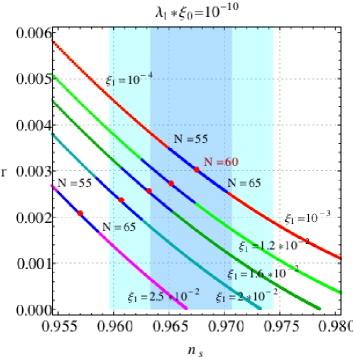
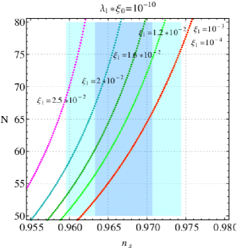
Figure 1: The potential $V(\sigma)$ for two fixed values of $\lambda_{1}\xi_{0}$ and with different $\xi_{1}$. The flat region is wide for a large range of $\sigma$, with the width controlled by $\gamma\sim 1/\sqrt{\xi}_{1}$ while its height is $V_{0}\propto 1/\xi_{0}$. We have $V/V_{\text{min}}\propto\xi_{1}^{2}/(\lambda_{1}\xi_{0})$.

Figure 2: The spectral index $n_{s}$ versus $r$ (left plot) and $n_{s}$ versus $N$ (right plot), for models with $\lambda_{1}\xi_{0}=10^{-10}$ and with different $\xi_{1}$. $N$ varies along each curve; in the left plot, on each curve of fixed $\xi_{1}$, the dark-blue curve has $N=55$ and $N=65$ at its left and right ends, respectively. The red dots correspond to $N=60$. The curves for $\xi_{1}=10^{-3}$ and $\xi_{1}=10^{-4}$ are nearly identical (saturated bound as $\xi_{1}\rightarrow 0$) in both plots. Blue (light blue) regions correspond to $n_{s}$ given by $n_{s}=0.9670\pm 0.0037$ at 68 $\%$ CL (95 $\%$ CL) respectively [51]. The constraint $r\!<\!0.07$ is easily satisfied. The value of $r$ is very small, below that of Starobinsky case: for $N=60$ we have $r\leq 0.00303$ (from top curve, saturated bound as $\xi_{1}\!\rightarrow\!0$) and $r\!>\!0.00257$ from the lower bound on $n_{s}$ ($68\%$ CL) with $\xi_{1}=1.6\times 10^{-2}$.

Eqs.(15) to (19) are used for a numerical study of the scalar spectral index $n_{s}$, the tensor-to-scalar ratio $r=16\,\epsilon_{*}$ and number of e-folds $N$, in terms of $\xi_{1}$ and $\lambda_{1}\xi_{0}$. We have

$$n_{s}=1+2\,\eta_{*}-6\,\epsilon_{*},$$ (20)

where the subscript $*$ stands for $\sigma=\sigma_{*}$.

Before discussing numerical results, we present simple analytical results for $n_{s}$ and $r$ in the limit $\lambda_{1}\xi_{0}\ll\xi_{1}^{2}\ll 1$. Therefore, we can keep only the leading term in expansion in $(\lambda_{1}\xi_{0})$, then expand in $\xi_{1}$. These results depend on $\xi_{1}$ only in this approximation. We find

$$\epsilon = \frac{1}{3}\,\,\xi_{1}^{2}\,\sinh^{2}\frac{2\sigma}{M\sqrt{6}}+{\cal O}(\xi_{1}^{3})\,$$ (21)

$$\eta = -\frac{2}{3}\,\xi_{1}\,\cosh\frac{2\sigma}{M\sqrt{6}}+{\cal O}(\xi_{1}^{2})\,$$ (22)

valid up to ${\cal O}(\lambda_{1}\xi_{0})$ corrections. Therefore

$$\qquad n_{s}\,=\,1-\frac{4}{3}\,\xi_{1}\,\cosh\frac{2\sigma_{*}}{M\sqrt{6}}+{\cal O}(\xi_{1}^{2})\,$$ (23)

The value of $n_{s}$ is controlled by $\eta$ in leading order ${\cal O}(\xi_{1})$ while $\epsilon$ contribution is subleading ${\cal O}(\xi_{1}^{2})$; hence we have a small tensor-to-scalar ratio $r=16\,\epsilon_{*}$. We then have

$$r=3\,(1-n_{s})^{2}+{\cal O}(\xi_{1}^{2})$$ (24)

This is an approximate result (valid only for smallest $\xi_{1}$) for the top curve shown in the left plot in Figure 2 (this figure actually uses the exact numerical results discussed later). As an example, if $n_{s}=0.968$ then $r\approx 0.003$. Increasing $\xi_{1}$ should reduce $n_{s}$ of (23) but there is implicit $\xi_{1}$-dependence in $\sigma_{*}$, computed below. First, we have

$${\cal N}(\sigma)=-\frac{3}{4\,\xi_{1}}\ln\tanh^{2}\frac{\sigma}{M\sqrt{6}}+\frac{3}{4}\ln\cosh^{2}\frac{\sigma}{M\sqrt{6}}+{\cal O}(\xi_{1}^{2})$$ (25)

Inflation ends at $\sigma=\sigma_{e}$ where

$$\sinh^{2}\frac{2\sigma_{e}}{M\sqrt{6}}=\frac{3}{\xi_{1}^{2}}+{\cal O}(\xi_{1}).$$ (26)

For example: $(\sigma_{e},\xi_{1})=(12.8M,10^{-4})$; $(7.16M,10^{-2})$. Then from (25), (26)

$${\cal N}(\sigma_{e})=\Big{[}\frac{\sqrt{3}}{2}+\frac{3}{8}\ln\frac{3}{4}\Big{]}-\frac{3}{4}\ln\xi_{1}+\frac{\sqrt{3}}{4}\xi_{1}+{\cal O}(\xi_{1}^{2}).$$ (27)

Using this result we find an iterative solution $\sigma_{*}$ to eq.(17) for a fixed $N$:

$$\tanh^{2}\frac{\sigma_{*}}{M\sqrt{6}} \approx 1-\frac{4\xi_{1}}{3}\,\overline{N},$$ (28)

where

$$\overline{N} = \Big{\{}N+{\cal N}(\sigma_{e})+\frac{3}{4}\ln\Big{[}\frac{4\xi_{1}}{3}\big{(}N+{\cal N}(\sigma_{e})\big{)}\Big{]}\Big{\}}+{\cal O}(\xi_{1}^{2}).$$ (29)

For $N=60$ then $\overline{N}\approx 64.1$ for $\xi_{1}$ between $10^{-4}$ and $10^{-3}$; for $N=55$ then $\overline{N}\approx 59.06$ for the same $\xi_{1}$ range. Finally, using $\sigma_{*}$ of (28) and (21), (23), we have approximate relations for $n_{s}$ and $r=16\,\epsilon_{*}$:

$$n_{s} = 1-\frac{2}{\overline{N}}+{\cal O}(\xi_{1})$$ (30)

$$r = \frac{12}{{\overline{N}}^{2}}+\frac{16}{\overline{N}}\,{\cal O}(\xi_{1})$$ (31)

which are consistent with (24) and accurate for $\xi\sim 10^{-3}$ for the $r$ values considered here.

Let us now analyse the exact numerical values of $n_{s}$, $r$, $N$, eqs.(15) to (20) and compare them with the experimental data. Figure 2 summarises the main results of the paper: we presented $n_{s}$ versus $r$ (left plot) and $n_{s}$ versus $N$ (right plot), for models with parametric constraint $\lambda_{1}\xi_{0}=10^{-10}$ and curves of different $\xi_{1}$. The curves for $\xi_{1}=10^{-3}$ and $\xi_{1}=10^{-4}$ or smaller are nearly identical (saturated bound) in both plots. $N$ varies along each curve in the plane $(n_{s},r)$, and the range of values from $N=55$ to $N=60$ is shown in dark blue for each curve. Regions in blue (light blue) show the experimental values of $n_{s}$ at $68\%$ ($95\%$ CL), respectively, where $n_{s}=0.9670\pm 0.0037$ ($68\%$ CL) from Planck 2018 (TT, TE, EE + low E + lensing + BK14 + BAO) [51]. These bounds on $n_{s}$ and $r$ are comfortably respected at $68\%$ CL for the values of $\xi_{1}$ shown.

Let us compare Figure 2 to a result of Starobinsky model in which for $N=55$ one has $n_{s}\approx 0.965$ and $r\approx 0.0034$ [54]. In our model, for the same $N$ we also have $r\approx 0.00345$ which is the largest $r$ in the model for $N=55$ (top curve in Figure 2). Therefore the values for $r$ of the Starobinsky model (recovered for $\xi_{1}\rightarrow 0$), are at the upper limit of those in our model. This is also indicated by approximate results (30), (31) which also apply to Starobinsky model but with replacement $\overline{N}\rightarrow N$. With $\overline{N}>N$ we see that for the same $N$, we expect a mildly larger $n_{s}$ and smaller $r$ than in Starobinsky model.

Figure 2 for $N=60$ gives a lower bound for $r$ from the experimental (lower) value of $n_{s}$ (at $68\%$ CL) quoted above and with $\xi_{1}=1.6\times 10^{-2}$; there is also an upper bound on $r$ from the smallest $\xi_{1}$ (saturated limit, top red curve) also giving the largest $n_{s}$:

$$N=60,\qquad 0.00257\leq r\leq 0.00303.$$ (32)

Similar bounds can be extracted for different $N$. To conclude, a small tensor-to-scalar ratio is predicted by this model. Such value will soon be tested experimentally [55, 56, 57].

Our predictions used a hierarchy of couplings $\lambda_{1}\!\ll\!\xi_{1}\!\ll\!\xi_{0}$. This hierarchy is stable under matter (scalar) quantum corrections to (3) due to ultraweak $\lambda_{1}$ required to satisfy (14): we have one-loop corrections $\delta\lambda_{1}\!\propto\!\lambda_{1}^{2}/\kappa;$ $\delta\xi_{1}\!\propto\!(\xi_{1}+1/6)\lambda_{1}/\kappa$ and $\delta\xi_{0}\!\propto\!(\xi_{1}+1/6)^{2}/\kappa$, with $\kappa=(4\pi)^{2}$, see e.g.[53] (Section 3.1). Therefore the relative $\lambda_{1}$ suppression factor can maintain this hierarchy since then $|\delta\lambda_{1}|\ll|\delta\xi_{1}|\ll|\delta\xi_{0}|$. Therefore matter quantum corrections to $r$ and $n_{s}$ are small (for the Starobinsky-Higgs model these are well below $2.5\%$ for $r$ and less than $1\sigma$ for $n_{s}$ for minimal values of $\lambda_{1}$ used here [53]).

4 Weyl-tensor corrections to Weyl inflation

The analysis so far was based on $L_{0}$ of (1) coupled to the inflaton. A most general Weyl quadratic gravity action can contain an additional term allowed by symmetry (6), [38, 39]

$$L_{1}=\frac{1}{\eta}\,\tilde{C}_{\mu\nu\rho\sigma}\tilde{C}^{\mu\nu\rho\sigma}=\frac{1}{\eta}\,\Big{[}C_{\mu\nu\rho\sigma}\,C^{\mu\nu\rho\sigma}+\frac{3}{2}\,F_{\mu\nu}^{2}\Big{]},$$ (33)

where $\tilde{C}_{\mu\nu\rho\sigma}$ ($C_{\mu\nu\rho\sigma}$) denotes the Weyl tensor of Weyl (Riemannian) geometry, respectively; in the second step we used an identity to rewrite the action in the Riemannian picture.

If present, $L_{1}$ modifies our previous results for $r$. The analysis proceeds as before, since the transformations applied to obtain eqs.(11), (12) from eq.(3) leave $L_{1}$ invariant. Therefore, the new Lagrangian is that of eq.(11) plus $L_{1}$. For this new Lagrangian, the corrections to $r$ induced by the Weyl tensor were studied in [58] to which we refer the reader for details. The Weyl tensor brings a quadratic action for tensor fluctuations and a modified sound speed $c_{t}$ given by $1/c_{t}^{2}-1=(2H^{2})/(\eta M^{2})$ [58] (see eqs.(2.10), (2.22), (2.24)). With a slow roll relation $H^{2}\!\approx V/(3M^{2})$, $V\!\approx\!V_{0}$, the corrected tensor-to-scalar ratio $r_{c}$ is then

$$r_{c}=r\,\Big{[}1+\frac{8}{\eta\,\xi_{0}}\Big{]}^{1/2},$$ (34)

where $r$ is the value in the absence of $L_{1}$ while $n_{s}$ is unchanged. The Weyl boson mass is as in eq.(8) but with $q^{2}\rightarrow q_{c}^{2}=q^{2}/(1-6q^{2}/\eta)>0$ where $q_{c}$ is the new corrected coupling of the gauge kinetic term which includes that from $L_{1}$; also $q_{c}^{2}\!<\!1$ if $\eta\!<\!0$ or $\eta\!>\!6q^{2}/(1-q^{2})$.

As expected, eq.(34) shows that the change of $r$ due to $L_{1}$ depends on the relative size of the perturbative couplings of the two quadratic terms, $\eta$ versus $1/\xi_{0}$, and equals $\theta=(r_{c}-r)/r\approx 4/(\eta\,\xi_{0})$ for $|\eta|\,\xi_{0}\gg 1$. Recalling that $\xi_{0}>6.89\times 10^{8}$, a relative change by $\theta$ requires $\eta\approx 6\times 10^{-9}/\theta$. A value $r_{c}\!<\!r$ ($r_{c}\!>\!r$) corresponds to a negative (positive) $\eta$, respectively. In the limit $L_{1}$ is absent (formally $|\eta|\rightarrow\infty$, $q$ fixed) then $r_{c}=r$ and $q_{c}=q$ which recovers our previous results. In the limit the gauge kinetic term comes solely from (33) i.e. $L_{0}$ contains only the $\tilde{R}^{2}$ term (formally $q\rightarrow\infty$, $\eta$ fixed) then one has $\eta=-6q_{c}^{2}<0$.

A significant change $\theta$ (e.g. $\theta=50\%$) of an already very small (and well below current experimental bounds) tensor-to-scalar ratio needs an ultraweak $|\eta|$ (correspondingly $\eta\!=\!1.2\!\times\!10^{-8}$), which induces an instability in the theory below Planck scale. This is because there is a spin-two ghost (or tachyonic) state in $L_{1}$ [16] of (mass)${}^{2}\propto\eta\,M^{2}$. Avoiding this instability below Planck scale means corrections to $r$ from $L_{1}$ are negligible.

5 Further remarks

A potential similar to that in Section 3 was encountered in a previous model [32] with Weyl local symmetry. What are the differences? In our model there is no torsion (Weyl connection coefficients are symmetric [38, 39]) but we have Weyl gauge symmetry and non-metricity, while in the model of [32] only torsion is present. Further, in [32] the “gauge” field (denoted ${\cal T}_{\mu}$) emerges from the trace over the torsion and replaces our $\omega_{\mu}$. However, an ansatz is made

$${\cal T}_{\mu}=\partial_{\mu}\phi$$ (35)

with $\phi$ a scalar field. Under this assumption the model is Weyl integrable i.e. Riemannian (see e.g.[52]) and then non-metricity is absent (${\cal T}_{\mu}$ being a “pure” gauge field). Due to (35) the gauge kinetic term of ${\cal T}_{\mu}$ is vanishing (no dynamics) and can be integrated out. Therefore, no geometrical Stueckelberg mass mechanism can take place. For this reason a flat (Goldstone) direction remains present in [32] and it has kinetic mixing with the inflaton. The results then depend on the dynamics of the flat direction. This has implications for inflation discussed in [32], where it is shown that a distinct field space geometry changes the slow-roll plateau, which can affect inflation. If the kinetic energy of the Goldstone is large it can dominate and a “kination” period predates the slow-roll inflation; this may have additional consequences (observable effects in the CMB on large angular scales) [32]. In our case there is no Goldstone (flat direction) left since it was eaten by the Weyl “photon” which becomes massive via Stueckelberg mechanism and eventually decouples, yet it impacts on the potential (compare (12) to (9)).

Weyl inflation has an advantage compared to the Starobinsky model in that it cannot contain higher dimensional/curvature operators like $\tilde{R}^{4}/M^{4}$, etc of unknown coefficients that could affect significantly the numerical predictions or the convergence of such an expansion (in powers of $\tilde{R}$), see [62] for a discussion. Unlike in the Starobinsky model, such higher dimensional operators and their corrections are forbidden by the Weyl gauge symmetry. One could think of such operators being suppressed instead by (powers of) the dilaton field (to preserve this symmetry) but this is not possible since this field is already “eaten” by the Weyl massive “photon”, to all orders in perturbation theory. Further, given the Weyl gauge symmetry, the model is allowed by black-hole physics, which is not the case of similar models of inflation with only global scale symmetry (global charges can be eaten by black holes which subsequently evaporate, e.g. [61]). Finally, compared to models of inflation with local scale invariance (no gauging) that have a ghost present when generating Planck scale spontaneously by the dilaton vev, this problem is not present in Weyl gravity action eq.(3).

6 Conclusions

We examined if the original Weyl quadratic gravity is suitable for inflation. This theory is based on Weyl conformal geometry and its gauged (local) scale symmetry (also called Weyl gauge symmetry) forbids the presence of any fundamental mass scale in the action. Its action undergoes spontaneous breaking via geometric Stueckelberg mechanism. In this way the Weyl “photon” of gauged dilatations becomes massive (mass $\sim qM$), after absorbing the Goldstone mode (compensator/dilaton) $\ln\phi_{0}$ which is the spin-0 mode propagated by the $\tilde{R}^{2}$ term in the action. The result in the broken phase is the Einstein-Proca action for the Weyl “photon” and a positive cosmological constant. If the initial action also has a non-minimal coupling $\xi_{1}$ to an additional scalar ($\phi_{1}$), a scalar potential is found after the Stueckelberg mechanism. This potential has a minimum for non-vanishing scalar vev that is triggered by the gravitational effects (non-minimal coupling) and is suitable for inflation. Since the Planck scale is emergent as the scale where Weyl gauge symmetry is broken, the presence of field values above this scale, needed for inflation, is actually natural in Weyl gravity. Moreover, the existence of a non-zero vev of the dilaton (fixing $M$) is actually a dynamical effect in a FRW universe. The study is also motivated by the fact that the action involves the square of the (Weyl) scalar curvature, which points to similarities to the successful Starobinsky model.

Our analysis shows that Weyl inflation predicts a specific, small tensor-to-scalar ratio ($r$) within a narrow range $0.00257\leq r\leq 0.00303$ for $N=60$ and with $n_{s}$ within $68\%$ (CL) of the experimental value. This range of values for $r$ will soon be tested experimentally; they are mildly smaller than those for same $N$ in the Starobinsky model $M^{2}R+R^{2}$ recovered in the limit of vanishing non-minimal coupling. Such value for $r$ is also an indirect test of the presence of the Weyl gauge symmetry.

Compared to the Starobinsky model, the Weyl model of inflation has the advantage that it does not contain higher order curvature terms (e.g. effective operators $R^{4}/M^{4}$, etc) that modify the predictions or question the convergence of a series expansion in curvature; such operators are forbidden in Weyl inflation by the underlying Weyl gauge symmetry. This is because this symmetry does not allow a mass scale be present in the Weyl action to suppress such operators, while the dilaton field that could in principle suppress them (while preserving this symmetry) was already “eaten” by the massive Weyl photon. Another advantage is that the Weyl gauge symmetry of this model is also allowed by black-hole physics, unlike the models with a global scale symmetry, while local scale invariant models (no gauging) have a notorious ghost dilaton present, when generating the Planck scale spontaneously (by the dilaton vev). Finally, the above predictions for $r$ and the spectral index $n_{s}$ are found for values of the non-minimal coupling $\xi_{1}$ in the perturbative regime. In this respect the situation is very different from Higgs inflation where a large coupling $\xi_{1}$ is actually required.

Note added in proof: While this work was being typewritten, preprint arXiv:1906.03415 appeared (10 June) which analyses (section 4) inflation in this model by using the two-field basis eq.(7) instead of our one-field formulation, eq.(12). The results are consistent and complementary.

References

- [1] F. Englert, C. Truffin and R. Gastmans, “Conformal Invariance in Quantum Gravity,” Nucl. Phys. B 117 (1976) 407.
- [2] M. Shaposhnikov and D. Zenhausern, “Quantum scale invariance, cosmological constant and hierarchy problem,” Phys. Lett. B 671 (2009) 162 [arXiv:0809.3406 [hep-th]].
- [3] D. M. Ghilencea, “Quantum implications of a scale invariant regularization,” Phys. Rev. D 97 (2018) no.7, 075015 [arXiv:1712.06024 [hep-th]].
- [4] D. M. Ghilencea, “Manifestly scale-invariant regularization and quantum effective operators,” Phys. Rev. D 93 (2016) no.10, 105006 [arXiv:1508.00595 [hep-ph]].
- [5] D. M. Ghilencea, Z. Lalak and P. Olszewski, “Standard Model with spontaneously broken quantum scale invariance,” Phys. Rev. D 96 (2017) no.5, 055034 [arXiv:1612.09120 [hep-ph]].
- [6] D. M. Ghilencea, Z. Lalak and P. Olszewski, “Two-loop scale-invariant scalar potential and quantum effective operators,” Eur. Phys. J. C 76 (2016) no.12, 656 [arXiv:1608.05336 [hep-th]].
- [7] S. Mooij, M. Shaposhnikov and T. Voumard, “Hidden and explicit quantum scale invariance,” Phys. Rev. D 99 (2019) no.8, 085013 [arXiv:1812.07946 [hep-th]].
- [8] M. E. Shaposhnikov and F. V. Tkachov, “Quantum scale-invariant models as effective field theories,” arXiv:0905.4857 [hep-th].
- [9] M. Shaposhnikov and K. Shimada, “Asymptotic Scale Invariance and its Consequences,” Phys. Rev. D 99 (2019) no.10, 103528 [arXiv:1812.08706 [hep-ph]].
- [10] M. Shaposhnikov and A. Shkerin, “Gravity, Scale Invariance and the Hierarchy Problem,” JHEP 1810 (2018) 024 [arXiv:1804.06376 [hep-th]].
- [11] R. Foot, A. Kobakhidze, K. L. McDonald and R. R. Volkas, “Poincaré protection for a natural electroweak scale,” Phys. Rev. D 89 (2014) no.11, 115018 [arXiv:1310.0223 [hep-ph]].
- [12] M. Shaposhnikov and D. Zenhausern, “Scale invariance, unimodular gravity and dark energy,” Phys. Lett. B 671 (2009) 187 [arXiv:0809.3395 [hep-th]].
- [13] D. Blas, M. Shaposhnikov and D. Zenhausern, “Scale-invariant alternatives to general relativity,” Phys. Rev. D 84 (2011) 044001 [arXiv:1104.1392 [hep-th]].
- [14] J. Garcia-Bellido, J. Rubio, M. Shaposhnikov and D. Zenhausern, “Higgs-Dilaton Cosmology: From the Early to the Late Universe,” Phys. Rev. D 84 (2011) 123504 [arXiv:1107.2163 [hep-ph]].
- [15] F. Bezrukov, G. K. Karananas, J. Rubio and M. Shaposhnikov, “Higgs-Dilaton Cosmology: an effective field theory approach,” Phys. Rev. D 87 (2013) no.9, 096001 [arXiv:1212.4148 [hep-ph]].
- [16] L. Alvarez-Gaume, A. Kehagias, C. Kounnas, D. Lüst and A. Riotto, “Aspects of Quadratic Gravity,” Fortsch. Phys. 64 (2016) no.2-3, 176 [arXiv:1505.07657 [hep-th]].
- [17] C. Kounnas, D. Lüst and N. Toumbas, “R2 inflation from scale invariant supergravity and anomaly free superstrings with fluxes,” Fortsch. Phys. 63 (2015) 12 [arXiv:1409.7076 [hep-th]].
- [18] M. Trashorras, S. Nesseris and J. Garcia-Bellido, “Cosmological Constraints on Higgs-Dilaton Inflation,” Phys. Rev. D 94 (2016) no.6, 063511 [arXiv:1604.06760 [astro-ph.CO]].
- [19] G. K. Karananas and J. Rubio, “On the geometrical interpretation of scale-invariant models of inflation,” Phys. Lett. B 761 (2016) 223 [arXiv:1606.08848 [hep-ph]].
- [20] I. Antoniadis, A. Karam, A. Lykkas and K. Tamvakis, “Palatini inflation in models with an term,” JCAP 1811 (2018) no.11, 028 [arXiv:1810.10418 [gr-qc]].
- [21] A. Karam, T. Pappas and K. Tamvakis, “Nonminimal Coleman–Weinberg Inflation with an term,” JCAP 1902 (2019) 006 [arXiv:1810.12884 [gr-qc]].
- [22] J. Rubio and M. Shaposhnikov, “Higgs-Dilaton cosmology: Universality versus criticality,” Phys. Rev. D 90 (2014) 027307 [arXiv:1406.5182 [hep-ph]].
- [23] S. Casas, G. K. Karananas, M. Pauly and J. Rubio, “Scale-invariant alternatives to general relativity. III. The inflation-dark energy connection,” Phys. Rev. D 99 (2019) no.6, 063512 [arXiv:1811.05984 [astro-ph.CO]].
- [24] P. G. Ferreira, C. T. Hill and G. G. Ross, “Scale-Independent Inflation and Hierarchy Generation,” Phys. Lett. B 763 (2016) 174 [arXiv:1603.05983 [hep-th]].
- [25] P. G. Ferreira, C. T. Hill and G. G. Ross, “Weyl Current, Scale-Invariant Inflation and Planck Scale Generation,” Phys. Rev. D 95 (2017) no.4, 043507 [arXiv:1610.09243 [hep-th]];
- [26] P. G. Ferreira, C. T. Hill and G. G. Ross, “No fifth force in a scale invariant universe,” Phys. Rev. D 95 (2017) no.6, 064038 [arXiv:1612.03157 [gr-qc]].
- [27] S. Vicentini, L. Vanzo and M. Rinaldi, “Scale-invariant inflation with one-loop quantum corrections,” Phys. Rev. D 99 (2019) no.10, 103516 [arXiv:1902.04434 [gr-qc]].
- [28] M. Rinaldi and L. Vanzo, “Inflation and reheating in theories with spontaneous scale invariance symmetry breaking,” Phys. Rev. D 94 (2016) no.2, 024009 [arXiv:1512.07186 [gr-qc]].
- [29] G. ’t Hooft, “Local conformal symmetry in black holes, standard model, and quantum gravity,” Int. J. Mod. Phys. D 26 (2016) no.03, 1730006; “A class of elementary particle models without any adjustable real parameters,” Found. Phys. 41 (2011) 1829 [arXiv:1104.4543 [gr-qc]]. “Probing the small distance structure of canonical quantum gravity using the conformal group,” arXiv:1009.0669 [gr-qc].
- [30] J. Beltran Jimenez, L. Heisenberg and T. S. Koivisto, “Cosmology for quadratic gravity in generalized Weyl geometry,” JCAP 1604 (2016) no.04, 046 [arXiv:1602.07287 [hep-th]].
- [31] Y. Tang and Y. L. Wu, “Weyl Symmetry Inspired Inflation and Dark Matter,” arXiv:1904.04493 [hep-ph].
- [32] A. Barnaveli, S. Lucat and T. Prokopec, “Inflation as a spontaneous symmetry breaking of Weyl symmetry,” JCAP 1901 (2019) no.01, 022 [arXiv:1809.10586 [gr-qc]].
- [33] M. de Cesare, J. W. Moffat and M. Sakellariadou, “Local conformal symmetry in non-Riemannian geometry and the origin of physical scales,” Eur. Phys. J. C 77 (2017) no.9, 605 [arXiv:1612.08066 [hep-th]].
- [34] H. Nishino and S. Rajpoot, “Implication of Compensator Field and Local Scale Invariance in the Standard Model,” Phys. Rev. D 79 (2009) 125025 [arXiv:0906.4778 [hep-th]].
- [35] H. C. Ohanian, “Weyl gauge-vector and complex dilaton scalar for conformal symmetry and its breaking,” Gen. Rel. Grav. 48 (2016) no.3, 25 [arXiv:1502.00020 [gr-qc]].
- [36] L. Smolin, “Towards a Theory of Space-Time Structure at Very Short Distances,” Nucl. Phys. B 160 (1979) 253.
- [37] R. Percacci, “Gravity from a Particle Physicists’ perspective,” PoS ISFTG (2009) 011 [arXiv:0910.5167 [hep-th]]. “The Higgs phenomenon in quantum gravity,” Nucl. Phys. B 353 (1991) 271 [arXiv:0712.3545 [hep-th]].
- [38] D. M. Ghilencea, “Stueckelberg breaking of Weyl conformal geometry and applications to gravity,” arXiv:1904.06596 [hep-th].
- [39] D. M. Ghilencea, “Spontaneous breaking of Weyl quadratic gravity to Einstein action and Higgs potential,” JHEP 1903 (2019) 049 [arXiv:1812.08613 [hep-th]].
- [40] D. M. Ghilencea, H. M. Lee, “Weyl gauge symmetry and its spontaneous breaking in Standard Model and inflation,” Phys. Rev. D 99 (2019) no.11, 115007 [arXiv:1809.09174 [hep-th]].
- [41] Hermann Weyl, Gravitation und elektrizität, Sitzungsberichte der Königlich Preussischen Akademie der Wissenschaften zu Berlin (1918), pp.465; (Einstein’s comment appended).
- [42] “Eine neue Erweiterung der Relativitätstheorie” (“A new extension of the theory of relativity”), Ann. Phys. (Leipzig) (4) 59 (1919), 101-133.
- [43] “Raum, Zeit, Materie”, vierte erweiterte Auflage. Julius Springer, Berlin 1921 “Space-time-matter”, translated from German by Henry L. Brose, 1922, Methuen & Co Ltd, London.
- [44] For a review on Weyl geometry, applications to model building and references, see E. Scholz, “The unexpected resurgence of Weyl geometry in late 20-th century physics,” Einstein Stud. 14 (2018) 261 [arXiv:1703.03187 [math.HO]]; “Paving the Way for Transitions—A Case for Weyl Geometry,” Einstein Stud. 13 (2017) 171 [arXiv:1206.1559 [gr-qc]]; “Weyl geometry in late 20th century physics,” arXiv:1111.3220 [math.HO].
- [45] W. Drechsler and H. Tann, “Broken Weyl invariance and the origin of mass,” Found. Phys. 29 (1999) 1023 [gr-qc/9802044].
- [46] E. C. G. Stueckelberg, “Interaction forces in electrodynamics and in the field theory of nuclear forces,” Helv. Phys. Acta 11 (1938) 299.
- [47] P. G. Ferreira, C. T. Hill and G. G. Ross, “Inertial Spontaneous Symmetry Breaking and Quantum Scale Invariance,” Phys. Rev. D 98 (2018) no.11, 116012 [arXiv:1801.07676 [hep-th]]. C. T. Hill, “Inertial Symmetry Breaking,” arXiv:1803.06994 [hep-th].
- [48] A. A. Starobinsky “A New Type of Isotropic Cosmological Models Without Singularity,” Phys. Lett. B 91 (1980) 99 [Phys. Lett. 91B (1980) 99] [Adv. Ser. Astrophys. Cosmol. 3 (1987) 130].
- [49] K. Hayashi and T. Kugo, “Everything About Weyl’s Gauge Field,” Prog. Theor. Phys. 61 (1979) 334. doi:10.1143/PTP.61.334
- [50] D. Gorbunov, V. Rubakov, “Introduction to the theory of the early Universe”, World Scientific, 2011.
- [51] Y. Akrami et al. [Planck Collaboration], “Planck 2018 results. X. Constraints on inflation,” arXiv:1807.06211 [astro-ph.CO].
- [52] I. Quiros, “Scale invariant theory of gravity and the standard model of particles,” E-print arXiv:1401.2643 [gr-qc].
- [53] D. M. Ghilencea, “Two-loop corrections to Starobinsky-Higgs inflation,” Phys. Rev. D 98 (2018) no.10, 103524 [arXiv:1807.06900 [hep-ph]].
- [54] C. Patrignani et al., Particle Data Group, Chin. Phys. C, 40, 100001 (2016).
- [55] K. N. Abazajian et al. [CMB-S4 Collaboration], “CMB-S4 Science Book, First Edition,” arXiv:1610.02743 [astro-ph.CO]. https://cmb-s4.org/
- [56] J. Errard, S. M. Feeney, H. V. Peiris and A. H. Jaffe, “Robust forecasts on fundamental physics from the foreground-obscured, gravitationally-lensed CMB polarization,” JCAP 1603 (2016) no.03, 052 [arXiv:1509.06770 [astro-ph.CO]].
- [57] A. Suzuki et al., “The LiteBIRD Satellite Mission - Sub-Kelvin Instrument,” J. Low. Temp. Phys. 193 (2018) no.5-6, 1048 [arXiv:1801.06987 [astro-ph.IM]].
- [58] D. Baumann, H. Lee and G. L. Pimentel, “High-Scale Inflation and the Tensor Tilt,” JHEP 1601 (2016) 101 [arXiv:1507.07250 [hep-th]].
- [59] A. Delhom, G. J. Olmo and M. Ronco, “Observable traces of non-metricity: new constraints on metric-affine gravity,” Phys. Lett. B 780 (2018) 294, [arXiv:1709.04249 [hep-th]] and references therein.
- [60] I. P. Lobo and C. Romero, “Experimental constraints on the second clock effect,” Phys. Lett. B 783 (2018) 306 [arXiv:1807.07188 [gr-qc]].
- [61] R. Kallosh, A. D. Linde, D. A. Linde and L. Susskind, “Gravity and global symmetries,” Phys. Rev. D 52 (1995) 912 [hep-th/9502069].
- [62] J. Edholm, “UV completion of the Starobinsky model, tensor-to-scalar ratio, and constraints on nonlocality,” Phys. Rev. D 95 (2017) no.4, 044004 [arXiv:1611.05062 [gr-qc]].
- [63] P. G. Ferreira, C. T. Hill, J. Noller and G. G. Ross, “Scale independent inflation,” arXiv:1906.03415 [gr-qc].