Analytic results of the excited electronic states at $\upsilon=1/3$ and the Laughlin-Jain microscopic wave function approaches

Abstract

In this work we studied the properties of a two-dimensional electronic gas subjected to a strong magnetic field and cooled at a low temperature. We reported exact analytical results of energies at the ground state. The results are for systems up to $N_{e}=10$ electrons calculated in the integer quantum Hall effect (IQHE) regime at the filling factor $\upsilon=1$. To accomplish the calculation we used the complex polar coordinates method. Note that the system of electrons in the quantum Hall regime relied heavily on the disk geometry for finite systems of electrons with arbitrary values of $N_{e}=2$ to $10$ particles. The results that we obtained by analytical calculations are in good agreement with those reported by Ciftja [Ciftja O., J. Math. Phys., 2011, 52, 122105], where the representation for certain integrals of products of Bessel functions is obtained. In the end, we have studied the composite fermions energies for the excited states for several systems at $\upsilon=1/3$ and the correspondence between the fractional quantum Hall effect (FQHE) and the IQHE.

Key words: analytical method, fractional quantum Hall effect (FQHE), integer quantum Hall effect (IQHE), Coulomb interaction, quantum Hall effect, 2D electron gas

PACS: 73.43.-f

Abstract

Ó äàíié ðîáîòi äîñëiäæåíî âëàñòèâîñòi äâîìiðíîãî åëåêòðîííîãî ãàçó, ÿêèé є ïiä äiєþ ñèëüíîãî ìàãíiòíîãî ïîëÿ i îõîëîäæåíèé ïðè íèçüêié òåìïåðàòóði. Ïîäàíî òîчíi àíàëiòèчíi ðåçóëüòàòè äëÿ åíåðãié â îñíîâíîìó ñòàíi. Öi ðåçóëüòàòè ñòîñóþòüñÿ ñèñòåì àæ äî $N_{e}$ = 10 åëåêòðîíiâ, îáчèñëåíi â ðåæèìi öiëîчèñåëüíîãî êâàíòîâîãî åôåêòà Ãîëà (IQHE) ïðè êîåôiöiєíòi çàïîâíåííÿ $\upsilon$ =1. Äëÿ çäiéñíåííÿ îáчèñëåíü âèêîðèñòàíî ìåòîä ñêëàäíèõ ïîëÿðíèõ êîîðäèíàò. Ñëiä çàóâàæèòè, ùî ñèñòåìà åëåêòðîíiâ ó ðåæèìi êâàíòîâîãî åôåêòó Ãîëà, çíàчíîþ ìiðîþ ñïèðàєòüñÿ íà ãåîìåòðiþ äèñêà äëÿ ñêiíчåíèõ ñèñòåì åëåêòðîíiâ ç äîâiëüíèìè çíàчåííÿìè $N_{e}$ âiä 2 äî 10 чàñòèíîê. Ðåçóëüòàòè, îòðèìàíi ç äîïîìîãîþ àíàëiòèчíèõ îáчèñëåíü, äîáðå óçãîäæóþòüñÿ ç ðåçóëüòàòàìè Чiôò’ÿ [Ciftja O., J. Math. Phys., 2011, 52, 122105], äå îòðèìàíî ïðåäñòàâëåííÿ äëÿ iíòåãðàëiâ äîáóòêiâ ôóíêöié Áåññåëÿ. I íàðåøòi, äîñëiäæåíî åíåðãi¿ êîìïîçèòíèõ ôåðìiîíiâ çáóäæåíèõ ñòàíiâ äëÿ äåêiëüêîõ ñèñòåì ïðè $\upsilon$ =1/3 òà âiäïîâiäíiñòü ìiæ äðîáîâèì êâàíòîâèì åôåêòîì Ãîëà (FQHE) i öiëîчèñåëüíèì êâàíòîâèì åôåêòîì Ãîëà (IQHE).

Ключовi слова: àíàëiòèчíèé ìåòîä, äðîáîâèé êâàíòîâèé åôåêò Ãîëà (FQHE), öiëîчèñåëüíèé êâàíòîâèé åôåêò Ãîëà (IQHE), êóëîíiâñüêà âçàєìîäiÿ, êâàíòîâèé åôåêò Ãîëà, 2D åëåêòðîííèé ãàç

1 Introduction

A discovery of the integer quantum Hall effect (IQHE) [1, 2] was the beginning of a big revolution in the field of condensed matter. It is interesting to study theoretically and numerically the phases of the integer and fractional quantum Hall effect (FQHE) in a two-dimensional geometry in order to consider various aspects of this problem. In this article, we give some details of the formalism used to treat the IQHE and FQHE problem on the disk geometry [3, 4, 5]. As an hypothesis, Laughlin (1983) [6] considers that the electrons are confined on the plane in a central symmetric potential, so that the Hall droplet forms a disk of uniform density in the volume with the correct density of states per unit area. This area $2\piup ml_{0}^{2}$ is a circle where the radius contains $m$ flux quanta.

We solved the problem of the motion of a confined two-dimensional electron in a uniform magnetic field. This field is perpendicular to the motion of electrons. That presumes that the electron system is fully spin polarized. The shape of the system is a disk. Let us first consider free electrons, for a homogeneous uniform magnetic field $\mathbf{B}=(0,0,B)$. The symmetric gauge is defined by the vector potential $\mathbf{A}$

$$\mathbf{A}=\frac{\mathbf{B}}{2}(-y,x,0)\text{.}$$ (1.1)

In this gauge, the vector potential $\mathbf{A}$ is invariant by rotation about the axis $z$, and in the canonical momentum $\mathbf{p}=-\text{i}\hbar\boldsymbol{\nabla}$. In the presence of a magnetic field, the Hamiltonian can be written as follows:

$$\mathbf{H}=\frac{1}{2m}\Big{(}\mathbf{p}+\frac{e_{0}}{c}\mathbf{A}\Big{)}^{2}\text{.}$$ (1.2)

By introducing the complex variables

$$z=\frac{x-\text{i}y}{l_{0}}\,,~{}~{}\ ~{}\ ~{}z^{\ast}=\frac{x+\text{i}y}{l_{0}}\,.$$ (1.3)

The characteristic magnetic length on the disk $l_{0}=\sqrt{\hbar/eB}$ that will be taken equal to 1. The wave function in the lowest Landau level ($n=0$) is denoted by $\Psi_{0,m}$

$$\Psi_{0,m}=\prod_{i<j}\left(z_{i}-z_{j}\right)^{m}\mathrm{e}^{-\sum_{i}|z_{i}|^{2}/4}\text{.}$$ (1.4)

Let us consider a system of finite size such as a disk of radius $R$, and we can count the number of states in the lowest Landau level included in this disk. The probability of presence of the state $\left|0,m\right\rangle$ is defined by

$$\left|\Psi_{0,m}(z,\overline{z})\right|^{2}=\frac{1}{2\piup 2^{m}l_{0}^{2}m!}\frac{r^{2m}}{l_{0}^{2m}}\mathrm{e}^{-\frac{r^{2}}{2l_{0}^{2}}}\text{.}$$ (1.5)

The wave functions in the lowest Landau level are simple monomials in $z$. Thus, any state in the lowest Landau level (LLL) is given by a polynomial equation dependent only on $z$. The probability of presence of the state $\left|0,m\right\rangle$ is maximal over a circle of radius $r_{m}$ = $\sqrt{2m}l_{0}$, such that the radial extension of the wave function is of the order of $l_{0}$. When $m$ increases, the particle moves symmetrically away from the origin. The last state inside the disk of radius $R$ corresponds to $m=R^{2}/2l_{0}^{2}$ electronic orbitals, which is also equal to the total number of states in this disk.

The very good approximation of the true fundamental of equation (harmonic oscillator) of our system is that of Laughlin, but is not exactly the wave function of this fundamental which is written for odd integer $m$ in equation (1.4). This wave function describes a filling state. The basic state used in our system is described by Laughlin [6] in terms of Slater determinant in the first quantification which could be used to guess a test wave function for the ground state of the fractional quantum Hall effect. We proceed to study the systems $N_{e}=10$ of the composite fermions (CF) wave functions and we have to compare them to the exact wave functions in the disk geometry.

This article deals with the physics of the path connecting the fractional quantum Hall effect to the integral quantum Hall effect. In section 2, the model of interaction as well as the Coulomb interaction are presented. In section 3, the method of analytical results for IQHE at $\upsilon=1$ is shown. In section 4, we study the excitations of the CF states. In section 5, we give the results of our calculus. The conclusion is presented in section 6.

2 Model of interaction

The many-electron system is described by the Hamiltonian

$$\widehat{H}=\widehat{K}+\widehat{V}\text{,}$$ (2.1)

where $\widehat{K}$ is the kinetic energy operator, $\hbar$ is reduced Planck’s constant, $\omega=e_{0}B/m$ is the cyclotron frequency, and the Coulomb interaction $\widehat{V}$ projected in the LLL is obtained starting from the electron-electron interaction, electron-background and the background-background potentials. When all electrons are confined in the LLL, their kinetic energy is then constant $\big{\langle}\frac{\widehat{K}}{N_{e}}\big{\rangle}=\frac{1}{2}\hbar\omega$ [7]. We consider $N_{e}=10$ electrons of charge ($-e_{0}$) embedded in a uniform neutralizing background disk of an area and a positive charge $N_{e}~{}e_{0}$. Moreover, the disk is a part of the $xy$ plane subjected to a strong uniform magnetic field, in the $z$ direction, $\mathbf{B}=Be_{z}$, and lower temperatures.

The total potential energy operator is defined by

$$\widehat{V}=\widehat{V}_{\text{ee}}+\widehat{V}_{\text{eb}}+\widehat{V}_{\text{bb}}\,,$$ (2.2)

with $\widehat{V}_{\text{ee}}$, $\widehat{V}_{\text{eb}}$ and $\widehat{V}_{\text{bb}}$ denoting the electron-electron, electron-background and the background-background interaction potentials, respectively. Their corresponding expressions are given by

$$\widehat{V}_{\text{ee}}=\sum_{i<j}^{N}\ \frac{e_{0}^{2}}{|r_{i}-r_{j}|}\,,$$ (2.3)

$$\widehat{V}_{\text{eb}}=-\rho\sum_{i=1}^{N}\int\limits_{S_{N}}\mathrm{d}^{2}r\ \frac{e_{0}^{2}}{|r_{i}-r|}\,,$$ (2.4)

$$\widehat{V}_{\text{bb}}=\frac{\rho^{2}}{2}\int\limits_{S_{N}}\mathrm{d}^{2}r\int\limits_{S_{N}}\mathrm{d}^{2}r^{\prime}\ \frac{e_{0}^{2}}{|r-r^{\prime}|}\,,$$ (2.5)

where $r_{i}$ (or $r_{j}$ ) indicate the electron vector position while $r$ and $r^{\prime}$ are background coordinates. $S_{N}$ is the area of the disk and $\rho$ is the density of the system (the number of electrons per unit area) that can also be defined by

$$\rho=\frac{\upsilon}{2\piup l_{0}^{2}}\,.$$ (2.6)

The integer quantum Hall effect is perfectly explained without invoking interactions: only non-interacting particles fully occupying Landau levels. The interaction is crucial for fractional quantum Hall effect. The many-body wave functions will be of the form of the equation (1.4). The theory of the CF is a generalization of those considered by Jain [8] with the found states at $\upsilon=p/(2pm+1)$ with integer $m$ and $p$. This theory of the composite fermions immediately describes the elementary collective excitations by the promotion of a CF towards the states in higher Landau levels [9].

$$\Psi^{\text{gs}}(z_{1},\dots,z_{N_{e}})=\mathcal{P}_{\text{LLL}}\ \prod_{j<k}\left(z_{j}-z_{k}\right)^{2s}\Phi_{n}^{\text{gs}}.$$ (2.7)

Here, $\Phi_{n}^{\text{gs}}$ represents the incompressible IQHE ground state at filling factor $\upsilon=1$ (for noninteracting electrons), and $\mathcal{P}_{\text{LLL}}$ is an operator that projects the state onto the LLL. The factor $\prod_{j<k}\left(z_{j}-z_{k}\right)^{2s}$ is the Jastrow factor, binds $2s$ vortices to each electron to convert it into a composite fermion (CF), for two vortices $s=1$ [7]. The method for LLL projection is given in appendix A.

$$\Phi_{n}^{\text{gs}}=\prod_{j<k}^{N_{e}}\left(z_{j}-z_{k}\right)\exp\Big{(}-\frac{1}{4}\sum_{i}^{N_{e}}|z_{i}|^{2}\Big{)}.$$ (2.8)

This can be compared directly with exact numerical diagonalization results to test the applicability of CF trial wave functions to the system in each sector with a given number of particles $N_{e}$ and angular momentum $L=mN_{e}(N_{e}-1)/2$, with the basis formed by antisymmetrized functions of the form (1.4). The background-background interaction potential $\widehat{V}_{\text{bb}}$ can be classically calculated without using the wave function of the electron system. Its value is simply determined by calculating the elementary defined integral (2.5) and is given by reference [10].

$$\big{\langle}\widehat{V}_{\text{bb}}\big{\rangle}=\frac{8N_{e}}{3\piup}\sqrt{\frac{\upsilon N_{e}}{2}}\frac{e_{0}^{2}}{l_{0}}\,.$$ (2.9)

For a given wave function $\Psi(r_{1},\dots,r_{N_{e}})$, these energies are determined using the following formulae

$$\big{\langle}\widehat{V}_{\text{ee}}\big{\rangle}=\frac{\left\langle\Psi\left|V_{\text{ee}}\right|\Psi\right\rangle}{\left\langle\Psi\left|\Psi\right.\right\rangle}\,,\,\,\,\,\,\big{\langle}\widehat{V}_{\text{eb}}\big{\rangle}=\frac{\left\langle\Psi\left|V_{\text{eb}}\right|\Psi\right\rangle}{\left\langle\Psi\left|\Psi\right.\right\rangle}\text{. }$$ (2.10)

The term $\widehat{V}_{\text{ee}}$ is written as follows:

$$\big{\langle}\widehat{V}_{\text{ee}}\big{\rangle}=\frac{N_{e}(N_{e}-1)}{2}\int\mathrm{d}^{2}r_{1}\dots\mathrm{d}^{2}r_{N_{e}}\ \frac{e_{0}^{2}}{|r_{1}-r_{2}|}\left|\Psi r_{1},\dots,r_{N_{e}}\right|^{2}\text{.}$$ (2.11)

Similarly, for the $\widehat{V}_{\text{eb}}$ interaction, we have

$$\big{\langle}\widehat{V}_{\text{eb}}\big{\rangle}=-\rho N_{e}\int\mathrm{d}^{2}r_{1}\dots\mathrm{d}^{2}r_{N_{e}}\left|\Psi r_{1},\dots,r_{N_{e}}\right|^{2}\int\limits_{S_{N}}\mathrm{d}^{2}r\ \frac{e_{0}^{2}}{|r_{1}-r|}\,,$$ (2.12)

with

$$\int\limits_{S_{N}}\mathrm{d}^{2}r\ \frac{e_{0}^{2}}{|r_{1}-r|}=2\piup R_{N}\int\limits_{0}^{\infty}\frac{\mathrm{d}q}{q}J_{1}(q)J_{0}\Big{(}\frac{q}{R_{N}}r_{1}\Big{)},$$ (2.13)

where is the $J_{n}(x)$ $n$-th order Bessel functions. A detailed description of the ground state obtained by an analytical method is given in our earlier works [11, 12].

3 Analytical results for IQHE at $\upsilon=1$

In this section, we obtain the analytical expressions for the total energy per particle (in units $e_{0}^{2}/l_{0}$) and related quantities corresponding to IQHE system of electrons in a disk geometry at $\upsilon=1$. The ground state interaction energy per particle can be written as follows:

$$\varepsilon=\varepsilon_{\text{ee}}+\varepsilon_{\text{eb}}+\varepsilon_{\text{bb}}\,,$$ (3.1)

where $\varepsilon=\big{\langle}\widehat{V}\big{\rangle}/N_{e}$ ,   $\varepsilon_{\text{ee}}=\big{\langle}\widehat{V}_{\text{ee}}\big{\rangle}/N_{e}$ ,   $\varepsilon_{\text{eb}}=\big{\langle}\widehat{V}_{\text{eb}}\big{\rangle}/N_{e}$ and $\varepsilon_{\text{bb}}=\big{\langle}\widehat{V}_{\text{bb}}\big{\rangle}/N_{e}$. The energy of the interaction between electrons-electrons, electrons-background and the background-background is given by

$N_{e}=2;\left\{\begin{array}[]{l}\varepsilon_{\text{ee}}=\frac{\sqrt{\piup}}{8}\frac{e_{0}^{2}}{l_{0}}=0.22155673\frac{e_{0}^{2}}{l_{0}}\\ \varepsilon_{\text{bb}}=0.49007013\frac{e_{0}^{2}}{l_{0}}\\ \varepsilon_{\text{eb}}=-\frac{\sqrt{2\piup}}{4e}[3I_{0}(1)+5I_{1}(1)]=-1.52705731\frac{e_{0}^{2}}{l_{0}}\\ \varepsilon=-0.45667421\frac{e_{0}^{2}}{l_{0}}\end{array}\right.$

$N_{e}=3;\left\{\begin{array}[]{l}\varepsilon_{\text{ee}}=\frac{87\sqrt{\piup}}{384}\frac{e_{0}^{2}}{l_{0}}=0.40157158\frac{e_{0}^{2}}{l_{0}}\\ \varepsilon_{\text{bb}}=1.03959573\frac{e_{0}^{2}}{l_{0}}\\ \varepsilon_{\text{eb}}=-\frac{\sqrt{2\piup}}{16}[9I_{0}\big{(}\frac{3}{2}\big{)}+41I_{1}\big{(}\frac{3}{2}\big{)}]=-1.92501490\frac{e_{0}^{2}}{l_{0}}\\ \varepsilon=-0.48384759\frac{e_{0}^{2}}{l_{0}}\end{array}\right.$

$N_{e}=4;\left\{\begin{array}[]{l}\varepsilon_{\text{ee}}=\frac{5147\sqrt{\piup}}{16384}\frac{e_{0}^{2}}{l_{0}}=0.55681274\frac{e_{0}^{2}}{l_{0}}\\ \varepsilon_{\text{bb}}=1.20042175\frac{e_{0}^{2}}{l_{0}}\\ \varepsilon_{\text{eb}}=\frac{\sqrt{2\piup}}{96}[79I_{0}(2)-515I_{1}(2)]=-2.25835527\frac{e_{0}^{2}}{l_{0}}\\ \varepsilon=-0.50112077\frac{e_{0}^{2}}{l_{0}}\end{array}\right.$

$N_{e}=5;\left\{\begin{array}[]{l}\varepsilon_{\text{ee}}=\frac{102819\sqrt{\piup}}{262144}\frac{e_{0}^{2}}{l_{0}}=0.69519780\frac{e_{0}^{2}}{l_{0}}\\ \varepsilon_{\text{bb}}=1.34211232\frac{e_{0}^{2}}{l_{0}}\\ \varepsilon_{\text{eb}}=\frac{5\sqrt{2\piup}}{768e^{5/2}}[851I_{0}\big{(}\frac{5}{2}\big{)}-1869I_{1}\big{(}\frac{5}{2}\big{)}]=-2.55064421\frac{e_{0}^{2}}{l_{0}}\\ \varepsilon=-0.51333409\frac{e_{0}^{2}}{l_{0}}\end{array}\right.$

$N_{e}=6;\left\{\begin{array}[]{l}\varepsilon_{\text{ee}}=\frac{15545879\sqrt{\piup}}{33554432}\frac{e_{0}^{2}}{l_{0}}=0.82118371\frac{e_{0}^{2}}{l_{0}}\\ \varepsilon_{\text{bb}}=1.47021039\frac{e_{0}^{2}}{l_{0}}\\ \varepsilon_{\text{eb}}=\frac{3\sqrt{2\piup}}{2560e^{3}}[16629I_{0}(3)-25397I_{1}(3)]=-2.81395015\frac{e_{0}^{2}}{l_{0}}\\ \varepsilon=-0.52255605\frac{e_{0}^{2}}{l_{0}}\end{array}\right.$

$N_{e}=7;\left\{\begin{array}[]{l}\varepsilon_{\text{ee}}=\frac{283985723\sqrt{\piup}}{536870912}\frac{e_{0}^{2}}{l_{0}}=0.93756539\frac{e_{0}^{2}}{l_{0}}\\ \varepsilon_{\text{bb}}=1.58800872\frac{e_{0}^{2}}{l_{0}}\\ \varepsilon_{\text{eb}}=\frac{7\sqrt{2\piup}}{92160~{}e^{7/2}}[775265~{}I_{0}\big{(}\frac{7}{2}\big{)}-1007359~{}I_{1}\big{(}\frac{7}{2}\big{)}]=-3.05541141\frac{e_{0}^{2}}{l_{0}}\\ \varepsilon=-0.52983730\frac{e_{0}^{2}}{l_{0}}\end{array}\right.$

$N_{e}=8;\left\{\begin{array}[]{l}\varepsilon_{\text{ee}}=\frac{81126302255\sqrt{\piup}}{137438953472}\frac{e_{0}^{2}}{l_{0}}=1.04622906\frac{e_{0}^{2}}{l_{0}}\\ \varepsilon_{\text{bb}}=1.69765273\frac{e_{0}^{2}}{l_{0}}\\ \varepsilon_{\text{eb}}=\frac{\sqrt{2\piup}}{1290240~{}e^{4}}[217069951~{}I_{0}(4)-260821371~{}I_{1}(\frac{7}{2})]=-3.27965711\frac{e_{0}^{2}}{l_{0}}\\ \varepsilon=-0.53577533\frac{e_{0}^{2}}{l_{0}}\end{array}\right.$

$N_{e}=9;\left\{\begin{array}[]{l}\varepsilon_{\text{ee}}=\frac{1424926487975\sqrt{\piup}}{2199023255552}\frac{e_{0}^{2}}{l_{0}}=1.14851739\frac{e_{0}^{2}}{l_{0}}\\ \varepsilon_{\text{bb}}=1.80063263\frac{e_{0}^{2}}{l_{0}}\\ \varepsilon_{\text{eb}}=\frac{3\sqrt{2\piup}}{2293760e^{\frac{9}{2}}}[358919853~{}I_{0}\big{(}\frac{9}{2}\big{)}-413936659I_{1}\big{(}\frac{9}{2}\big{)}]=-3.48988824\frac{e_{0}^{2}}{l_{0}}\\ \varepsilon=-0.54073822\frac{e_{0}^{2}}{l_{0}}\end{array}\right.$

$N_{e}=10;\left\{\begin{array}[]{l}\varepsilon_{\text{ee}}=\frac{395560272250157\sqrt{\piup}}{562949953421312}\frac{e_{0}^{2}}{l_{0}}=1.24542568\frac{e_{0}^{2}}{l_{0}}\\ \varepsilon_{\text{bb}}=1.89803345\frac{e_{0}^{2}}{l_{0}}\\ \varepsilon_{\text{eb}}=\frac{5\sqrt{2\piup}}{10616832~{}e^{5}}[\text{2751387571}~{}I_{0}(5)-\text{3098794619}I_{1}(5)]=-3.68842587\frac{e_{0}^{2}}{l_{0}}\\ \varepsilon=-0.54496674\frac{e_{0}^{2}}{l_{0}}\,.\end{array}\right.$

4 The quasielectron ($qe$) energies

Nowadays, there are two universally accepted theories in the field of FQHE, the theory of Laughlin [6] and the theory of Jain [8]. An early trial wave function proposed by Laughlin for the ground state at the filling factor $\upsilon=1/m$, $m$ odd, turned out to work well [13]. The CF theory applies to a broader range of phenomena, while also providing a new interpretation for the physics of the $\upsilon=1/m$ state, as a state of CF at an effective filling of $\upsilon^{*}=1$ [8, 13]. While the wave function for the $\upsilon=1/m$ ground state from the CF theory is the same as that in reference [6], the wave functions for the excitations are different, which gives an opportunity to test the validity of the CF theory at $\upsilon=1/m$ itself. We note that when speaking of “quasielectrons” in this paper, we really mean “quasielectron excitations” of an incompressible FQHE state. Our objective in this work is to compare the two theories for systems containing $(N_{e}-1)qe$.

4.1 Laughlin’s $N_{e}-1$ quasielectron wave function

We concentrate herein below on $\upsilon$ = 1/3, with one quasielectron in the disk geometry. Note that the wave function $\Psi_{\text{L}}^{(N_{e}-1)qe}$ corresponding to the $(N_{e}-1)$ quasielectron states of Laughlin to the filling factor $\upsilon=1/3$. The trick of piercing a flux quantum adiabatically through the system motivates the following wave functions for the quasielectron[6]

$$\Psi_{\text{L}}^{(N_{e}-1)qe}=\Psi_{m}^{-z_{0}}=\exp\left(-\sum_{j}\ \frac{|z_{j}|^{2}}{4}\right)\left[\prod_{i=1}^{N_{e}-1}\Bigg{(}\frac{\partial}{\partial z_{i}}-\frac{z_{0}}{l_{0}^{2}}\Bigg{)}\right]\Bigg{[}\prod_{j<k}\left(z_{j}-z_{k}\right)^{m}\Bigg{]}.$$ (4.1)

In physics, this equation describes the creation of $(N_{e}-1)$ quasielectrons located at the origin.

4.2 The compact states [1,1, …,1]

In this subsection, we have used only one consequence of the CF theory for the quasiparticules in occupation [1,1, …,1] presented in [13, 14, 15, 16]. The CF basis consists of Jain wave function [17], where the derivatives do not act on the Gaussian factor [15], and one will derive only the polynomial part of the wave function from. The composite fermion wave function for the quasiparticle at $\upsilon=1/3$ is then given by

$${\tiny\Psi}_{\text{CF}}^{1qe}{\tiny=P}_{\text{LLL}}{\tiny\ }\prod_{j<k}^{N}\left(z_{j}-z_{k}\right)^{2}\left|\begin{array}[]{ccccc}\overline{z}_{1}&\overline{z}_{2}&\cdot&\cdot&\overline{z}_{N_{e}}\\ 1&1&\cdot&\cdot&1\\ z_{1}&z_{2}&\cdot&\cdot&z_{N_{e}}\\ \cdot&\cdot&\cdot&\cdot&\cdot\\ \cdot&\cdot&\cdot&\cdot&\cdot\\ z_{1}^{N_{e}-2}&z_{2}^{N_{e}-2}&\cdot&\cdot&z_{N_{e}}^{N_{e}-2}\end{array}\right|{\mathrm{e}}^{-\sum_{j=1}^{N}|z_{j}|^{2}/4},$$ (4.2)

and the CF wave function for the $N_{e}-1$ quasiparticle at $\upsilon=\frac{1}{3}$ is then given by

$${\tiny\Psi}_{\text{CF}}^{\left[1,...,1\right]}{\tiny=P}_{\text{LLL}}{\tiny\ }\prod_{j<k}^{N}\left(z_{j}-z_{k}\right)^{2}\left|\begin{array}[]{cccc}(\overline{z}_{1})^{N_{e}-1}&(\overline{z}_{2})^{N_{e}-1}&\cdot&(\overline{z}_{N_{e}})^{N_{e}-1}\\ (\overline{z}_{1})^{N_{e}-2}&(\overline{z}_{2})^{N_{e}-2}&\cdot&(\overline{z}_{N_{e}})^{N_{e}-2}\\ \cdot&\cdot&\cdot&\cdot\\ (\overline{z}_{1})^{2}&(\overline{z}_{2})^{2}&\cdot&(\overline{z}_{N_{e}})^{2}\\ \overline{z}_{1}&\overline{z}_{2}&\cdot&\overline{z}_{N_{e}}\\ 1&1&\cdot&1\end{array}\right|{\mathrm{e}}^{-\sum_{j=1}^{N}|z_{j}|^{2}/4}.$$ (4.3)

We have studied the Laughlin and CF energies for the excited states for several systems at $\upsilon=1/3$ and the correspondence between the FQHE and the IQHE. These energies are given in table 1, where $V_{\text{L}}$ represents the electron-electron interaction energy of Laughlin’s wave function, $V_{\text{CF}}$ is the electron-electron interaction energy of Jain’s wave function, and $V_{\text{Exact}}$ is the electron-electron interaction energy of exact analytical expressions [18].

Table 1: Comparison between the energy of Laughlin wave function and the energy of the CF wave function in disk geometry. Energies are in units of $e_{0}^{2}/l_{0}$ .

${}_{{}^{\text{CF}}}$	${}_{{}^{\text{1~{}qe}\equiv\text{[}N_{e}-1,1]}}$		${}_{{}^{\text{2~{}qe}\equiv\text{[}N_{e}-2,1,1]}}$		${}_{{}^{\text{3~{}qe}\equiv\text{[}N_{e}-3,1,1,1]}}$		${}_{{}^{\text{4~{}qe}\equiv\text{[}N_{e}\text{-4,1,1,1,1]}}}$
${}_{N_{e}}$	${V}_{\text{L}}$	${V}_{\text{CF}}$	${V}_{\text{L}}$	${V}_{\text{CF}}$	${V}_{\text{L}}$	${V}_{\text{CF}}$	${V}_{\text{L}}$	${V}_{\text{CF}}$
2	0.443114	0.443114	-	-	-	-	-	-
3	0.891204	0.891204	1.20472	1.20472	-	-	-	-
4	1.50139	1.50172	1.78598	1.78512	2.22725	2.22725	-	-
5	2.24874	2.24905	2.53811	2.53707	2.92117	2.91876	3.47599	3.47599
6	3.11368	3.11219	3.42216	3.41913	3.79696	3.79441	4.26863	4.26452
7	4.08010	4.07622	4.41587	4.40773	4.80306	4.79646	5.25455	5.27973
${}_{{}^{\text{CF}}}$	${}_{{}^{\text{5~{}qe}\equiv[N_{e}-5,1,1,1,1,1]}}$		${}_{{}^{\text{6~{}qe}\equiv\text{[1,1,1,1,1,1,1]}}}$		${}_{{}^{\text{IQHE}}}$
${}_{N_{e}}$	${V}_{\text{L}}$	${V}_{\text{CF}}$	${V}_{\text{L}}$	${V}_{\text{CF}}$	${V}_{\text{Exact}}$[18]
2	-	-	-	-	0.443114
3	-	-	-	-	1.20472
4	-	-	-	-	2.22725
5	-	-	-	-	3.47599
6	4.92710	4.92710	-	-	4.92710
7	5.80798	5.80254	6.56296	6.56296	6.56296

Our study confirms the description of quasielectrons as (CF) in an excited (CF) quasi-Landau level. This wave function contains one excited (CF) in the second CF quasi-Landau level but the other in the $(N_{e}-1)$ CF quasi-Landau level, as indicated by the notation $[1,1,\dots,1]$.

5 Results and discussion

Within this work, we considered two systems. The first one for the ground energy with up to $N_{e}=10$ electrons at the filling $\upsilon=1$ and the second one for the exited energy with up to $N_{e}=7$ electrons at the filling $\upsilon=1/3$. Several researchers used the disk geometry in their works [3, 5, 6, 11]. The mathematical derivations as well as the Mathematica code [19] are used to calculate the interaction energy to perform the analytical method for $N_{e}=7$ particles. The code of the electron-background interaction energy computation $\varepsilon_{\text{eb}}$ is shown in appendix B.

This result is consistent with previous studies, the Laughlin wave function for $N_{e}$ quasiparticle is increased and approaches about Jain states in occupation [1,1, …,1]. Figure 1 shows that the energies of $Nqe$ quasielectrons for $N_{0}=2$ to 7 particles, in the disk geometry for $\upsilon=1/3$, and the FQHE are equal to those for the IQHE, where we denote the compact states by [$N_{0}$, $N_{1}$, …, $N_{7}$], where one composite fermion occupied one Landau level [14, 15].

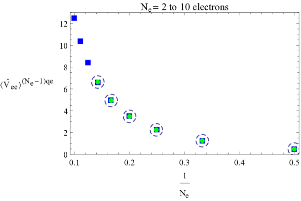
Figure 1: (Colour online) The $N_{e}-1$ quasielectron energies for $N_{e}=7$ in disk geometry at $\upsilon=1/3$. The green thickness represents Laughlin’s states $\Psi$${}_{\text{L}}$$\mathbb{}^{(N_{e}-1)qp}$. The dashed circle represents Jain’s states $\Psi$${}_{\text{CF}}$$\mathbb{}^{[1,1,\ldots\,,1]}$. The blue rectangle represents IQHE states at $\upsilon=1$.

In figure 1, we can see that the results derived by the present exact analytical calculation at the filling $\upsilon=1$ and $\upsilon=1/3$ (the excited states) compare well with the results of [18] obtained using the method of Exact analytic solutions. For $N_{e}$ quasiparticles, the energies for $N_{e}=7$ in disk geometry at $\upsilon=1/3$ of Laughlin states correspond to occupation [1,1, …,1] of Jain states.

6 Conclusion

We conclude that the analytical expression for the Coulomb interaction energy in disk geometry at filling factor 1/3 permits us to obtain a correspondence between the fractional quantum Hall effect and the integer quantum Hall effect. The coinciding energies of the IQHE and the $(N_{e}-1)$ quasielectron of the FQHE states are expected, where the FQHE and the IQHE can be unified. The FQHE is explained as the IQHE of composite fermions. This physics not only gives the best available microscopic wave functions for the quasiparticles but also brings out new qualitative structures for multi-quasiparticle states. These quasiparticles may be classified in theory as composite fermions, which allows us to understand the fractional quantum hall effect of electrons as an integer quantum hall effect of these composite fermions.

Appendix A Lowest Landau level projection operator $\mathcal{P}_{\text{LLL}}$

In the CF theory, the wave function for the ground state $\Psi^{\text{GS}}$ at $\upsilon=1/3$ takes the form [8]

$$\Psi^{\text{GS}}(z_{1},\dots,z_{N_{e}})=\mathcal{P}_{\text{LLL}}\ \prod_{j<k}\left(z_{j}-z_{k}\right)^{2}\Phi_{1}\,,$$ (A.1)

where $\Phi_{1}$ represents the wave function of noninteracting electrons

$$\Phi_{1}=\prod_{j<k}^{N}\left(z_{j}-z_{k}\right)\exp\bigg{(}-\frac{1}{4}\sum_{i}^{N}|z_{i}|^{2}\bigg{)}\text{.}$$ (A.2)

The CF wave function for one quasielectron (1$qe$) at $\upsilon=1/3$ is then given by

$$\Psi_{\text{CF}}^{1qp}=\mathcal{P}_{\text{LLL}}\ \prod_{j<k}^{N}\left(z_{j}-z_{k}\right)^{2}\left|\begin{array}[]{ccccc}\overline{z}_{1}&\overline{z}_{2}&\cdot&\cdot&\overline{z}_{N}\\ 1&1&\cdot&\cdot&1\\ z_{1}&z_{2}&\cdot&\cdot&z_{N}\\ \cdot&\cdot&\cdot&\cdot&\cdot\\ z_{1}^{N-2}&z_{2}^{N-2}&\cdot&\cdot&z_{N}^{N-2}\end{array}\right|\exp\bigg{(}-\frac{1}{4}\sum_{j}^{N}|z_{j}|^{2}\bigg{)}\,.$$ (A.3)

The $\mathcal{P}_{\text{LLL}}$ is an operator that projects the state onto the lowest Landau level, where the LLL projection of any wave function can be obtained by normal ordering the wave function followed by replacing $\overline{z}_{i}\rightarrow 2\partial/\partial z_{i}$, where the derivatives do not act on the Gaussian factor.

For example, for $N_{e}$ $=4$ electrons

$$\Psi_{\text{CF}}^{1qp}=\mathcal{P}_{\text{LLL}}\ \prod_{j<k}^{N}\left(z_{j}-z_{k}\right)^{2}\left|\begin{array}[]{cccc}\overline{z}_{1}&\overline{z}_{2}&\overline{z}_{3}&\overline{z}_{4}\\ 1&1&1&1\\ z_{1}&z_{2}&z_{3}&z_{4}\\ z_{1}^{2}&z_{2}^{2}&z_{3}^{2}&z_{4}^{2}\\ z_{1}^{3}&z_{2}^{3}&z_{3}^{3}&z_{4}^{3}\end{array}\right|\exp\bigg{(}-\frac{1}{4}\sum_{j}^{N}|z_{j}|^{2}\bigg{)}\,,$$ (A.4)

where

$$\Phi_{1}^{{}^{\prime}} = \prod_{j<k}^{N}\left(z_{j}-z_{k}\right)^{2}$$ (A.5)

$$= (z_{1}-z_{2})^{2}(z_{1}-z_{3})^{2}(z_{2}-z_{3})^{2}(z_{1}-z_{4})^{2}(z_{2}-z_{4})^{2}(z_{3}-z_{4})^{2}\text{.}$$

The CF basis functions of LLL projected wave functions $\Psi_{\text{CF}}^{1qp}$, then take the following form:

$$\Psi_{\text{CF}}^{1qp} = \bigg{(}z_{2}^{2}z_{3}\frac{\partial\Phi_{1}^{{}^{\prime}}}{\partial z_{1}}-z_{2}z_{3}^{2}\frac{\partial\Phi_{1}^{{}^{\prime}}}{\partial z_{1}}-z_{2}^{2}z_{4}\frac{\partial\Phi_{1}^{{}^{\prime}}}{\partial z_{1}}+z_{3}^{2}z_{4}\frac{\partial\Phi_{1}^{{}^{\prime}}}{\partial z_{1}}+z_{2}z_{4}^{2}\frac{\partial\Phi_{1}^{{}^{\prime}}}{\partial z_{1}}$$ (A.6)

$$-z_{3}z_{4}^{2}\frac{\partial\Phi_{1}^{{}^{\prime}}}{\partial z_{1}}-z_{1}^{2}z_{3}\frac{\partial\Phi_{1}^{{}^{\prime}}}{\partial z_{2}}+z_{1}z_{3}^{2}\frac{\partial\Phi_{1}^{{}^{\prime}}}{\partial z_{2}}+z_{1}^{2}z_{4}\frac{\partial\Phi_{1}^{{}^{\prime}}}{\partial z_{2}}-z_{3}^{2}z_{4}\frac{\partial\Phi_{1}^{{}^{\prime}}}{\partial z_{2}}$$

$$-z_{1}z_{4}^{2}\frac{\partial\Phi_{1}^{{}^{\prime}}}{\partial z_{2}}+z_{3}z_{4}^{2}\frac{\partial\Phi_{1}^{{}^{\prime}}}{\partial z_{2}}+z_{1}^{2}z_{2}\frac{\partial\Phi_{1}^{{}^{\prime}}}{\partial z_{3}}-z_{1}z_{2}^{2}\frac{\partial\Phi_{1}^{{}^{\prime}}}{\partial z_{3}}-z_{1}^{2}z_{4}\frac{\partial\Phi_{1}^{{}^{\prime}}}{\partial z_{3}}$$

$$+z_{2}^{2}z_{4}\frac{\partial\Phi_{1}^{{}^{\prime}}}{\partial z_{3}}+z_{1}z_{4}^{2}\frac{\partial\Phi_{1}^{{}^{\prime}}}{\partial z_{3}}-z_{2}z_{4}^{2}\frac{\partial\Phi_{1}^{{}^{\prime}}}{\partial z_{3}}-z_{1}^{2}z_{2}\frac{\partial\Phi_{1}^{{}^{\prime}}}{\partial z_{4}}+z_{1}z_{2}^{2}\frac{\partial\Phi_{1}^{{}^{\prime}}}{\partial z_{4}}$$

$$+z_{1}^{2}z_{3}\frac{\partial\Phi_{1}^{{}^{\prime}}}{\partial z_{4}}-z_{2}^{2}z_{3}\frac{\partial\Phi_{1}^{{}^{\prime}}}{\partial z_{4}}-z_{1}z_{3}^{2}\frac{\partial\Phi_{1}^{{}^{\prime}}}{\partial z_{4}}+z_{2}z_{3}^{2}\frac{\partial\Phi_{1}^{{}^{\prime}}}{\partial z_{4}}\bigg{)}\mathrm{e}^{-[(z_{1}^{2}+z_{2}^{2}+z_{3}^{2}+z_{4}^{2})/4]}\,.$$

Appendix B The $\varepsilon_{\text{eb}}$ calculation

(*SetDirectory["directory name"]*)
SetDirectory["C:\Users\Hmida\Desktop\4-particles-electron-background"];
Directory[];
Module[{Ne, Nu, R, SN, Rho, Polyz, CoefPoly, CoefPolyMin, PolyExpand,
RePoly, CoefPolyList, Clist, Inner1, Inlist, I1, I2, I3, I5, I6,
DenomiIntegralr1, SumDenomi, SumNomi, Ke, KeN, KeM, CoefPoly1, SumGloVeb,
EnergyVeb, strm}, Ne = 4;Nu = 1;R = l[0]*Sqrt[2*Ne/Nu];SN = Pi*R^2;
Rho = Nu/(2*Pi*l[0]^2);
Polyz = Product[Product[(z[i] - z[j]), {j, i + 1, Ne}], {i, 1, Ne - 1}];
CoefPoly = Exponent[Polyz, z[1]];
CoefPolyMin = Exponent[Polyz, z[1], Min];
PolyE = Expand[Polyz];
RePoly = Flatten[Table[ Coefficient[PolyE, z[1], i], {i, CoefPolyMin,CoefPoly}]];
CoefPolyList = Plus @@ Select[RePoly, #1 =!= 0 &];
Clist = CoefPolyList /. Plus -> List;
Inner1 = Inner[Times, Clist /. {z[2] -> 1, z[3] -> 1, z[4] -> 1}, Clist, Plus];
Inlist = Inner1 /. Plus -> List /. {z[2] -> r[2]^2, z[3] -> r[3]^2,
z[4] -> r[4]^2};
I1 = Integrate[ Inlist*r[2]*r[3]*Exp[-r[3]^2/(2 l[0]^2)], {r[3], 0, Infinity},
Assumptions -> (l[0] > 0)];
I2 = Integrate[ I1*Exp[-r[2]^2/(2 l[0]^2)], {r[2], 0, Infinity},
Assumptions -> (l[0] > 0)];
I3 = Integrate[ I2*r[4]*Exp[-r[4]^2/(2 l[0]^2)], {r[4], 0, Infinity},
Assumptions -> (l[0] > 0)] /. Plus -> List;
Ke = 0;KeN = 0;KeM = 0;CoefPoly1 = CoefPoly + 1;
Do[
I5 = Times[I3, i];
Ke = Ke + I5;
I6 = Integrate[ r[1]^(2 i - 1)*Exp[-r[1]^2/(2 l[0]^2)], {r[1], 0, Infinity},
Assumptions -> (l[0] > 0)];
KeN = KeN + I6;
KeM = KeM + FunctionExpand[(2 l[0]^2)^i*MeijerG[{{1}, {1}}, {{1/2, i}, {-1/2}},
Ne*Nu]/4],{i, 1, CoefPoly1}];
NomiIntegralr1 = Reverse[Plus @@ Ke /. Plus -> List];
KeN = Plus @@ Flatten[KeN] /. Plus -> List;
KeM = N[Plus @@ Flatten[KeM]] /. Plus -> List;
SumNomi = N[Plus @@ Flatten[ Inner[Times, NomiIntegralr1, KeM, Plus]]];
SumDenomi = N[Flatten[ Inner[Times, NomiIntegralr1, KeN, Plus]]];
SumGloVeb = Divide[SumNomi, SumDenomi];
EnergyVeb = N[Times[SumGloVeb, (-2*Rho*SN/R) e[0]^2], 8];
strm = OpenWrite["EnergyVeb"];
Write[strm, EnergyVeb];
Close[strm];
Print[EnergyVeb];] // Timing -2.25835527 e[0]^2/l[0].

Ukrainian 0

Àíàëiòèчíi ðåçóëüòàòè çáóäæåíèõ åëåêòðîííèõ ñòàíiâ ïðè $\upsilon=1/3$ òà ìåòîäè Ëàôëiíà-Äæåéíà ìiêðîñêîïiчíî¿ õâèëüîâî¿ ôóíêöi¿ M.A. Aììàð

             
Ëàáîðàòîðiÿ ôiçèêè åêñïåðèìåíòàëüíèõ ìåòîäiâ i ¿õ çàñòîñóâàíü, Óíiâåðñèòåò Ìåäå¿, Àëæèð

References

\@nopatterns
Ukrainian \adddialect\l@ukrainian0 \l@ukrainian