Controllability of Kronecker Product Networks
Abstract
A necessary and sufficient condition is derived for the controllability of Kronecker product networks, where the factor networks are general directed graphs. The condition explicitly illustrates how the controllability of the factor networks affects the controllability of the composite network. For the special case where at least one factor network is diagonalizable, an easily-verifiable condition is explicitly expressed. Furthermore, the controllability of higher-dimensional multi-agent systems is revisited, revealing that some controllability criterion reported in the literature does not hold. Consequently, a modified necessary and sufficient condition is established. The effectiveness of the new conditions is demonstrated through several examples.
keywords:
Network controllability, network observability, Kronecker product graph, multi-agent systems., , ,
1 Introduction
Controllability is a fundamental issue to be addressed before considering how to control a dynamical system in applications [6]. This subject has been extensively studied over more than half a century with various criteria developed, such as the PBH test, Kalman and other kinds of rank conditions, substantial graphic properties, and so on [10, 13, 24].
For most large-scale networked systems, these criteria cannot be applied practically because of their complex structures and heavy computational burdens. Therefore, in recent years, the notion of network controllability has received compelling attention with some efficient criteria established [15, 17, 18, 19, 12, 1, 23, 27, 25, 9, 28, 30, 31, 32, 33, 34]. In [31], an exact controllability framework was introduced to identify the minimum set of input nodes for a general network with an arbitrary link-weight distribution. The controllability of networks with specific topologies, such as path graphs, cycle graphs, circulant graphs, multi-chain graphs and grid graphs, was explored in [17, 18, 19, 12]. Network controllability was investigated from a graph-theoretic perspective in [21, 32, 1, 23]. It is noted that most of the above results are derived for the networks with one-dimensional nodes. Recently, the controllability of networks with higher-dimensional nodes has attracted a great deal of interest [9, 25, 27, 28, 30, 32, 33, 34]. Some controllability conditions for networked LTI systems were presented in [34, 33], which depend on the transmission zeros of every subsystem and the connection matrix. The controllability of diffusively coupled LTI systems was studied in [32] and [27]. In [25], the controllability condition for networked MIMO systems was established in terms of two algebraic matrix equations. Moreover, some easily-verifiable conditions were proposed in [9, 28] for the controllability of networked LTI systems with a diagonalizable topology matrix.
Besides isolated networks, composite networks have come into play due to their broad applications in different areas of engineering [8, 16]. There are many kinds of composite networks, such as Cartesian product networks, Kronecker product networks, strong product networks, lexicographic product networks and so on. In addition to their importance of constructing ‘larger’ networks out of ‘small’ ones, they are useful in the sense that one can get insights about the properties of composite networks from the factor networks. Intuitively, the controllability of a composite network might be verified by checking some properties of the factor networks. The controllability and observability of Cartesian product networks were investigated in [5]. In [18], the controllability and observability of linear dynamical systems whose dynamics are induced by the Laplacian of a grid graph were studied. Note that many real-world networks are similar to stochastic Kronecker product graphs. For example, the Kronecker power of a simple generating matrix can yield a Kronecker product graph that fits the Internet (at the autonomous systems level) fairly well [14]. Large online social networks, web and blog graphs, peer-to-peer networks, etc., can also be modeled by Kronecker product networks. Moreover, every non-trivial graph has a prime factorization over the Kronecker product [8, 16]. It has lower computational complexity to check the controllability of a large-scale network by examining some properties of the smaller factor networks. Therefore, the controllability analysis for Kronecker product networks has brought about renewed interest recently [2, 4, 29, 11]. The eigenanalysis for the Kronecker product of two matrices was presented in [11], which shows that the Kronecker products of the factor matrices’ eigenvectors are the eigenvectors of the composite matrix. However, not all the eigenvectors of the composite matrix are formulated therein. In [29], the Kronecker product of defective matrices was revisited, characterizing the number of the eigenvectors. Nevertheless, the explicit expressions of the eigenvectors, which are the cornerstone of controllability analysis, are not presented. Recently, a sufficient condition was established in [4] for the controllability of Kronecker product networks, where the topology matrices are required to be diagonalizable.
In this paper, the controllability of Kronecker product networks is revisited. The contribution of the paper is four-fold. First, the factor networks considered here are general, directed and weighted. Differing from the condition given in [4], which requires the topology matrix of the composite network to be diagonalizable, this paper removes the diagonalizability requirement. Second, a new necessary and sufficient condition on the controllability of Kronecker product networks is provided in terms of eigenvectors. Compared with the classical PBH test, the new condition typically has a much lower computational cost. Third, for the special case where at least one factor network is diagonalizable, a specified condition is explicitly expressed, which is easier to verify. Finally, this paper shows that the sufficiency of the controllability criterion given in [3] does not hold, thereby a modified necessary and sufficient condition is derived.
The remainder of this paper is organized as follows. Some notations and preliminaries are given in Section 2. The model is formulated in Section 3. Some conditions on the controllability of Kronecker product networks are developed in Section 4. The controllability of higher-dimensional multi-agent systems is reinvestigated in Section 5. Finally, conclusions are drawn in Section 6.
2 Notations and Preliminaries
In this section, notations and useful preliminaries are introduced.
2.1 Notations
The notations mostly follow [9]. Let be the row vector with all zero entries except for . The linear span of row vectors , , is a set of all the linear combinations of these vectors, i.e., . Let be the direct sum of two spaces and . Matrices, if their dimensions are not explicitly indicated, are assumed to be compatible for algebraic operations.
A weighted digraph is characterized by a node set with cardinality , an edge set comprised of ordered pairs of nodes with cardinality , and a weight set with cardinality , where an edge exists from nodes to if with edge weight . is called the adjacency matrix of with if and otherwise. The th diagonal term of the adjacency matrix denotes the weight of the self-loop on node .
2.2 Kronecker Product Network
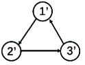
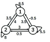
The Kronecker product network is a kind of composite network that can be obtained by applying Kronecker product operation(s) to several smaller networks, called factor networks. Let and be two factor networks. The Kronecker product of and , denoted by , has the node set . There is an edge from node to node if and only if is an edge of and is an edge of . If an edge exists, the corresponding weight is . An example of the Kronecker product of two graphs and is displayed in Fig. 1.

2.3 Useful Lemmas and Definitions
Lemma 1.
[22] If , , , are linearly independent vectors and , , , are arbitrary vectors, then implies that for all . Moreover, the roles of and in the above statement can be exchanged.
Definition 1.
[22] A row vector is called the th-order generalized left eigenvector of matrix corresponding to its eigenvalue if , and . Moreover, , , form a left Jordan chain of on top of , where the maximum value of is called the length of this Jordan chain.
3 Model Formulation
Consider a network consisting of nodes with a directed and weighted topology in the following form [7, 20, 14]:
| (1) |
where is the state of node , represents the coupling strength between nodes and , is the control input to node , and if node is under control, but otherwise , for all . Assume that if there is an edge from node to node , otherwise , for all . Denote and , which represent the topology and the external input channels of the network (1), respectively. Let be the whole state of the network, and be the total external control input. Then, the network (1) can be rewritten in a compact form as
| (2) |
In the following, consider the controllability of the network with topology graph being the Kronecker product of two factor graphs and . The dynamics of the factor networks are described by and , where and are the state vector and the control input of the first factor network, respectively; and are the state vector and the control input of the second factor network, respectively. According to the definition of Kronecker product graph, it is easy to prove . Therefore, for this Kronecker product network, its compact form can be formulated as (2) with
| (3) |
The analysis here is presented in terms of two factor networks, which can be extended to larger numbers of factor networks by sequential compositions. In the following, it will be shown that the controllability of the composite network can be revealed by examining some features of the smaller factor networks, which makes the computational complexity much lower.
Remark 1.
A graph is prime if it is nontrivial and cannot be decomposed into the Kronecker product of two nontrivial graphs. An expression , with each being prime, is called a prime factorization of . Note that every nontrivial graph has a prime factorization over the Kronecker product [8]. It has lower computational complexity to check the controllability of a large-scale network by examining some properties of the smaller factor networks. Therefore, exploring low-dimensional controllability conditions for Kronecker product networks is of great significance in engineering applications, which gives insight into the controllability of large-scale networks.
4 Main Results
In this section, controllability conditions for the composite network (2)-(3) are considered. Firstly, the general case that both and are non-diagonalizable is investigated. Then, a special case where at least one factor network is diagonalizable is further analyzed, with a direct and easily-verifiable condition derived.
4.1 Both and are non-diagonalizable
In this subsection, the general case that both and are non-diagonalizable is investigated. The connection between the eigenspaces of the factor networks and that of the composite network provides a mechanism to establish efficient controllability conditions. Firstly, all left eigenvectors of the Kronecker product of two defective matrices are characterized.
Theorem 1.
Let and be two defective matrices, where and are nilpotent matrices. The eigenvalues of are . Moreover,
-
•
if , the corresponding left eigenvectors are , , , , where , , , ;
-
•
if and , the corresponding left eigenvectors are , ;
-
•
if and , the corresponding left eigenvectors are , ;
-
•
if , the corresponding left eigenvectors are , , , , , , .
Proof: According to the structure of matrix , it is easy to verify that the eigenvalues of are . In the following, the aforementioned four cases are proved respectively.
Case : . Since , it follows that is the left eigenvector of . Note that is the left eigenvector of if and only if
| (4) |
This implies that . Since and , equation (4) holds, indicating that is the left eigenvector of .
Assume that , , are the left eigenvectors of . Then, is the left eigenvector of if and only if
| (5) |
Since and one can verify that (5) holds. Therefore, is the left eigenvector of . It has been shown in [29] that the number of the left eigenvectors for this case is , thus all the left eigenvectors of are , , .
Case : and . Since , it follows that is the left eigenvector of , . It has been shown in [29] that the number of the left eigenvectors for this case is , thus all the left eigenvectors of are , , .
One can prove the results in Cases and similarly, thus the detail is omitted. This completes the proof.
Remark 2.
The number of the eigenvectors of associated with the sole eigenvalue was given in [29]. However, it does not present explicit expressions of the eigenvectors, which are characterized in the above theorem. Theorem 1 is the cornerstone of the following controllability analysis for Kronecker product networks.
In what follows, the left eigenvectors of are expressed through the generalized eigenspaces of the factor networks.
Theorem 2.
Let be the eigenvalues of , and be the eigenvalues of . Then, the eigenvalues of are , , , , , , . Moreover, for the eigenvalue with geometric multiplicity ,
-
•
if , then , and the corresponding left eigenvectors are , ;
-
•
if and , then , and the corresponding left eigenvectors are , ;
-
•
if and , then , and the corresponding left eigenvectors are , ;
-
•
if and , then , and the corresponding left eigenvectors are , , , , , ,
where , , is the left Jordan chain of associated with the eigenvalue , and , , is the left Jordan chain of associated with the eigenvalue , , .
Proof: Let be a nonsingular matrix such that , where is the Jordan form of and the th Jordan block with being a nilpotent matrix, . The left Jordan chain of associated with the eigenvalue is denoted as , , , , where is the top vector and is the length of the Jordan chain.
Let be a nonsingular matrix such that , where is the Jordan form of and the th Jordan block , . The left Jordan chain of associated with the eigenvalue is denoted as , , , , where is the top vector and is the length of the Jordan chain.
Since , the eigenvalues of are , , , , , , . Let and . It is easy to derive that . If is a left eigenvector of , then is the left eigenvector of , , . Thus, the results follow from Theorem 1 directly.
The explicit expressions of the left eigenvectors given in Theorem 2 are the core of the following controllability criteria for Kronecker product networks. Let be the left eigenspace of corresponding to the eigenvalue . In what follows, a theorem is established for the controllability of the Kronecker product network (2)-(3).
Theorem 3.
Proof: Using Theorem 2 and the PBH test, one can prove this theorem easily. Thus, the detail is omitted.
Remark 3.
Theorem 3 provides a precise and efficient criterion for determining the controllability of a general Kronecker product network, using the generalized eigenvectors of the factor networks with low dimensions. Compared with the classical PBH test, the new condition typically has a much lower computational cost. Due to linear systems duality, the results in Theorem 3 are equally applicable to the observability of Kronecker product networks.
The effectiveness of the above condition can be illustrated by the following example.
Example 1.
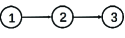
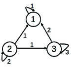
Consider graph depicted in Fig. 2.
It is easy to verify that . The eigenvalues of are , . The left eigenvector associated with is and the left Jordan chain corresponding to is , . It is easy to obtain that is non-diagonalizable. Assume that the second node of is under control. Thus, one has . Let , . Then and . If , one has . It then follows from Theorem 3 that is uncontrollable. This example fully demonstrates the effectiveness of the condition.
Remark 4.
Theorem in [4] has established a controllability condition for Kronecker product networks, which requires to be diagonalizable. This assumption is conservative and the condition can only be applied to a very restricted type of networks. The new condition here removes this restriction, thus is more general and flexible. This nontrivial extension is of great significance in engineering applications.
In the following, some more intuitive and easily-verifiable conditions are presented, which reveal how the controllability of the factor networks affects the controllability of the whole composite network.
Corollary 1.
Corollary 2.
Proof: If has an eigenvalue , without loss of generality, let , then the left eigenvectors of corresponding to are , , , , , , , where is the left eigenvector of associated with the eigenvalue ; , , , , , , are all the left root vectors of . If the composite network (2)-(3) is controllable, then , for any scalars , , , , , , , which are not all zero. That is, , which implies , for any nonzero . Since , , , , , , are all the left root vectors of , which span , one has .
The second part can be proved similarly.
Hereinafter, the special case where or is diagonalizable is analyzed in detail, for which a simple and effective condition is obtained. Compared with the conditions for the general case, this easy-to-verify condition allows to check the network controllability more efficiently.
4.2 or is diagonalizable
In this subsection, a controllability criterion is established for the Kronecker product network (2)-(3) with one diagonalizable factor network.
Corollary 3.
Assume that or is diagonalizable. Let be the set of the eigenvalues of , and be the set of the eigenvalues of . The composite network (2)-(3) is controllable if and only if the following four conditions hold simultaneously:
-
1.
and are controllable;
-
2.
if has an eigenvalue , then ;
-
3.
if has an eigenvalue , then ;
-
4.
if , where , , for , , then , , are linearly independent, where is the left eigenvector of corresponding to the eigenvalue ; is the left eigenvector of corresponding to the eigenvalue , .
Proof: The case that is diagonalizable is firstly proved. In this case, . Then with a similar method, one can prove the other case easily.
Necessity: First of all, from Corollaries 1 and 2, it follows that conditions - are necessary for the controllability of the composite network (2)-(3).
Assume that , where , , , . Then, any left eigenvector of corresponding to can be expressed in the form of , where is the left eigenvector of corresponding to the eigenvalue ; is the left eigenvector of corresponding to the eigenvalue ; are some scalars which are not all zero. If the composite network (2)-(3) is controllable, then . Consequently, , for any scalars , , , which are not all zero. Therefore, , , are linearly independent.
Sufficiency: One needs to prove that, if the composite network (2)-(3) is uncontrollable, then at least one condition in Corollary 3 does not hold. Based on the PBH test, if the composite network (2)-(3) is uncontrollable, then there exists a left-eigenpair of , denoted as , such that
| (6) |
This will be discussed in the following cases.
-
•
If is an eigenvalue with the geometric multiplicity being , assume that , it then follows from Theorem 2 that , where with the corresponding left eigenvector ; with the corresponding left eigenvector . From equality (6), it can be easily deduced that , which yields or . It can be then derived that is uncontrollable or is uncontrollable.
-
•
If is an eigenvalue with the geometric multiplicity more than , assume that , where , , , . It follows from Theorem 2 that can be expressed in the form of , where is the left eigenvector of associated with the eigenvalue ; is the left eigenvector of associated with the eigenvalue ; are some scalars, which are not all zero. From equality (6), it follows that there exists a nonzero vector , such that It indicates that , , are linearly dependent.
-
•
If , assume that and . It follows from Theorem 2 that can be expressed in the form of , where is the left eigenvector of associated with the eigenvalue , ; , () are defined as in Theorem 2; and are some scalars, which are not all zero. From equality (6), it follows that there exist scalars and , which are not all zero, such that , which implies that
(7) From Lemma 1, it can be derived that equality (7) holds if and only if at least one of the following conditions holds:
-
1.
, , , , , , are linearly dependent.
-
2.
, , are linearly dependent.
Since , , , , , , are all the left root vectors of , which span , the first condition implies that . Moreover, since , , are all the left eigenvectors of , which span , the second condition indicates that . Thus, in this case, if the composite network (2)-(3) is uncontrollable, then or .
-
1.
Therefore, if the composite network (2)-(3) is uncontrollable, then at least one condition in Corollary 3 does not hold. This completes the proof.
The effectiveness of this criterion can be illustrated by the following example.
Example 2.
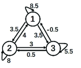
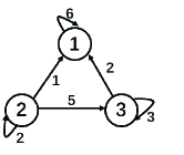
Consider two graphs and , which are depicted in Fig.3.
It is easy to verify that and . Note that is diagonalizable. The eigenvalues of are , and with the corresponding left eigenvectors , and , respectively. Moreover, the eigenvalues of are , . The left eigenvector associated with is and the left Jordan chain corresponding to is , . Assume that the first two nodes of have control inputs and all the nodes of are under control. Thus, one has and . Firstly, it is easy to verify that and are controllable. Since has an eigenvalue and , the second condition holds. Further, noting that , one needs to check whether and are linearly dependent. Since , and are linearly independent. Moreover, and . Thus, one can verify that and are linearly independent. It then follows from Corollary 3 that is controllable. This result coincides with the conclusion derived by the Kalman rank condition.
If is diagonalizable, then both and are diagonalizable. The conditions in Corollary 3 are also effective for diagonalizable Kronecker product networks, as demonstrated by the following example.
Example 3.
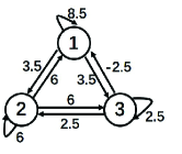
Consider two graphs and , which are depicted in Fig. 4.
It is easy to verify that and . The eigenvalues of are , and with the corresponding left eigenvectors , and , respectively. The eigenvalues of are , and with the corresponding left eigenvectors , , , respectively. It is easy to verify that is diagonalizable. Assume that the first two nodes of have control inputs. Node and node of are under control. Thus, one has and . Both pairs and are controllable. Since , the value of is required to be checked, which gives , for any nonzero . It then follows from Corollary 3 that is controllable, which coincides with the conclusion derived by the Kalman rank condition. This example fully demonstrates the effectiveness of the condition.
Remark 5.
A controllability criterion for diagonalizable Kronecker product networks was established in [4], which was claimed to be necessary and sufficient. However, Example 3 shows that the necessity of that criterion does not hold. Corollary 3 provides a new controllability condition, which is not only sufficient but also necessary.
5 Controllability of Higher-dimensional Multi-agent Systems Revisited
5.1 Problem Statement
Consider a multi-agent system consisting of agents labeled by the set . Assign the roles of leaders and followers to the agents by denoting and as the sets of indices of the leaders and followers, respectively, where .
To each follower , associate a dynamical system , and to each leader , we associate a dynamical system , where is the state of agent ; is the external input to agent ; is the coupling input from other agents.
Agent is said to be a neighbor of agent if its state is known by agent . Here, assume that the neighboring relationships are fixed, which can be described by a directed and weighted graph . The coupling input to each agent is determined by the diffusive coupling rule based on the neighboring relations as follows: , where is the matrix describing inner-coupling between different components, and is the strength of the information link.
The Laplacian matrix of and the external input channels of the multi-agent system are denoted by and , respectively, where for , but otherwise , for all . Let be the whole state of the multi-agent system, and be the total external control input. Then, the above multi-agent system can be rewritten in a compact form as
| (8) |
with
| (9) |
Note that matrix has the form of the Kronecker product of two matrices and so does . This higher-dimensional multi-agent system can be seen as a special case with being a Laplacian matrix. In the following, conditions for ensuring the controllability of the multi-agent system (8)-(9) are specified.
Remark 6.
The controllability of networked LTI systems or multi-agent systems with linear dynamics has been investigated in [32, 9, 27, 28, 30]. The state matrices for those systems have the form of rather than a pure Kronecker product. The higher-dimensional multi-agent systems investigated here can be seen as a special case with nodes having no internal dynamics.
5.2 A Counterexample
Recall the controllability condition for the multi-agent system (8)-(9) given in [3], where it was assumed that the first agents are leaders. Then, and can be partitioned as , where and with subscripts ‘l’ and ‘f’ denoting ‘leader’ and ‘follower’, respectively.
Theorem 4.
However, while this condition is necessary for the controllability of the network, it may not be sufficient, as shown in the following example.
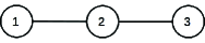
Consider the undirected path network with three nodes depicted in Fig. 5. Node is selected to be the leader. One has and . Let and . It is easy to verify that and are controllable. From Theorem in [3], it follows that this undirected path network is controllable.
However, if one checks the controllability of this system by using the classical Kalman rank condition, one can find that is actually uncontrollable. Therefore, its sufficiency does not hold.
This example is a modification of the example presented in [27], which was used to demonstrate that the controllability condition for diffusive networks proposed in [32] is not always sufficient. The incomplete eigenanalysis of networks presented in [32] and [3] leads to errors in controllability analysis. In the following, a modified controllability condition is proposed, which is both necessary and sufficient.
5.3 New Controllability Criteria
Note that the conditions proposed in Section 4 are not restricted to checking the controllability of Kronecker product networks. They can tackle the controllability problem for any system represented by the Kronecker product of two matrices. Based on the results in Section 4, a modified controllability condition for the multi-agent system (8)-(9) is established as follows.
Corollary 4.
Proof: Note that has an eigenvalue . If the multi-agent system (8)-(9) is controllable, then . From Corollaries 1 and 2, it follows that the conditions (1) and (3) are necessary for the controllability of the multi-agent system (8)-(9).
For sufficiency, one needs to prove that, if the conditions (1)-(3) hold, then no left eigenvectors of are orthogonal to , thus the multi-agent system (8)-(9) is controllable. It is easy to verify that if the conditions (1)-(3) hold, then no left eigenvectors of associated with eigenvalue are orthogonal to . For a nonzero eigenvalue , if it is not a common eigenvalue, it follows from Theorem 2 that any corresponding left eigenvector can be expressed as , where , , is the left Jordan chain of associated with the eigenvalue , and , , is the left Jordan chain of associated with the eigenvalue , , is a nonzero scalar about and , , , are scalars, which are not all zero. Next, the value of will be checked. It is easy to verify that . Since , , , are linearly independent. Since is controllable, it follows that and are not all zero. From Lemma 1, it can be easily deduced that . Thus, for any nonzero eigenvalue of , if it is not a common eigenvalue, no corresponding left eigenvectors are orthogonal to . Similarly, one can prove that, for each nonzero common eigenvalue of , no corresponding left eigenvectors are orthogonal to . Consequently, no left eigenvectors of are orthogonal to . Therefore, the multi-agent system (8)-(9) is controllable. This completes the proof.
According to Corollary 4, one can easily verify that the undirected path network in the above counterexample is uncontrollable. This example fully demonstrates the effectiveness of the condition.
6 Conclusions
The controllability of Kronecker product networks has been investigated, in which the factor networks have general directed topologies. A necessary and sufficient condition for the controllability of the composite network has been derived, which is effective and has a much lower computational cost as compared to existing criteria. For the special case where at least one factor network is diagonalizable, a specified condition has also been established, which is simple and easier to verify. Moreover, the controllability of higher-dimensional multi-agent systems has been reinvestigated. It is found that the sufficiency of the controllability criterion given in [3] does not hold. Consequently, a modified condition is derived, which is necessary and sufficient. In future studies, the controllability and observability of other types of network-of-networks will be further considered.
References
- [1] Aguilar, C. O., & Gharesifard, B. (2017). Almost equitable partitions and new necessary conditions for network controllability. Automatica, 80, 25–31.
- [2] Asavathiratham, C., Roy, S., Lesieutre, B., & Verghese, G. (2001). The influence model. IEEE Control Systems Magazine, 21(6), 52–64.
- [3] Cai, N., Zhang, Y. S. (2010). Formation controllability of high-order linear time-invariant swarm systems. IET Control Theory and Applications, 4(4), 646–654.
- [4] Chapman, A., Mesbahi, M. (2014). Kronecker product of networked systems and their approximates. In 21st International Symposium on the Mathematical Theory of Networks and Systems. Groningen, the Netherlands (pp. 1426–1431).
- [5] Chapman, A., Nabi-Abdolyousefi, M., & Mesbahi, M. (2014). Controllability and observability of network-of-networks via Cartesian products. IEEE Transactions on Automatic Control, 59(10), 2668–2679.
- [6] Chen, G. R. (2017). Pinning control and controllability of complex dynamical networks. International Journal of Automation and Computing, 14(1), 1–9.
- [7] Chen, G. R., Wang, X. F., & Li, X. (2014). Fundamentals of Complex Networks: Models, Structures and Dynamics. Wiley Press.
- [8] Hammack, R., Imrich, W., & Klavzar, S. (2011). Handbook of Product Graphs. CRC Press.
- [9] Hao, Y. Q., Duan, Z. S., & Chen, G. R. (2018). Further on the controllability of networked MIMO LTI systems. International Journal of Robust and Nonlinear Control, 28(5), 1778–1788.
- [10] Hautus. M. L. J. (1969). Controllability and observability conditions of linear autonomous systems. Nederlandse Akademie van Wetenschappen Proceedings Series A-Mathematical Sciences, 72(5), 443–448.
- [11] Horn, R. A., & Johnson, C. R. (1991). Topics in matrix analysis. Cambridge, U.K.: Cambridge Univ. Press.
- [12] Hsu, S.-P. (2017). A necessary and sufficient condition for the controllability of single-leader multi-chain systems. Int. J. Robust Nonlinear Control, 27(1), 156–168.
- [13] Kalman, R. E. (1962). Canonical structure of linear dynamical systems. Proceedings of the National Academy of Sciences of the United States of America, 48(4), 596–600.
- [14] Leskovec, J. (2010). Kronecker graphs: an approach to modeling networks. Journal of Machine Learning Research, 11, 985–1042.
- [15] Liu, Y. Y., Slotine, J. J., & Barabasi, A. L. (2011). Controllability of complex networks. Nature, 473(7346), 167–173.
- [16] Loan, C. F. Van (2000). The ubiquitous Kronecker product. Journal of Computational and Applied Mathematics, 123, 85–100.
- [17] Nabi-Abdolyousefi, M., & Mesbahi, M. (2013). On the controllability properties of circulant networks. IEEE Transactions on Automatic Control, 58(12), 3179–3184.
- [18] Notarstefano, G., & Parlangeli, G. (2013). Controllability and observability of grid graphs via reduction and symmetries. IEEE Transactions on Automatic Control, 58(7), 1719–1731.
- [19] Parlangeli, G., & Notarstefano, G. (2012). On the reachability and observability of path and cycle graphs. IEEE Transactions on Automatic Control, 57(3), 743–748.
- [20] Pasqualetti, F., Zampieri, S., & Bullo, F. (2014). Controllability metrics, limitations and algorithems for complex networks. IEEE Transactions on Network Systems, 1(1), 40–52.
- [21] Rahmani, A., Ji, M., Mesbahi, M. & Egerstedt, M. (2009). Controllability of multi-agent systems from a graph-theoretic perspective. SIAM Journal on Control and Optimization, 48(1), 162–186.
- [22] Roman, M. (2005). Advanced Linear Algebra. New York: Springer.
- [23] Sun, C., Hu, G. Q., & Xie, L. H. (2017). Controllability of multi-agent networks with antagonistic interactions. IEEE Transactions on Automatic Control, 62(10), 5457–5462.
- [24] Trentelman, H., Stoorvogel, A. A., & Hautus, M. (2012). Control Theory for Linear Systems. New York: Springer.
- [25] Wang, L., Chen, G. R., Wang, X. F., & Tang, W. K. S. (2016) Controllability of networked MIMO systems. Automatica, 69, 405–409.
- [26] Weichsel, P. M (1962). The Kroneker product of graphs. Proceedings of the American Mathematical Society, 13(1), 47–52.
- [27] Xue, M. R., & Roy, S. (2018). Comments on “Upper and lower bounds for controllable subspaces of networks of diffusively coupled agents”. IEEE Transactions on Automatic Control, 63(7), 2306.
- [28] Xue, M. R., & Roy, S. (2017). Input-output properties of linearly-coupled dynamical systems: Interplay between local dynamics and network interactions. In 56th IEEE conference on decision and control. Melbourne, Australia (pp. 487–492).
- [29] Xue, M. R., & Roy, S. (2012). Kronecker products of defective matrices: some spectral properties and their implications on observability. In 2012 American Control Conference. Montreal, Canada (pp. 5202–5207).
- [30] Xue, M. R., & Roy, S. (2018). Modal barriers to controllability in networks with linearly-coupled homogeneous subsystems. arXiv preprint arXiv:1805.01995.
- [31] Yuan, Z. Z., Zhao, C., Di, Z. R., Wang, W. X., & Lai, Y. C. (2013). Exact controllability of complex networks. Nature Communication, 4, 2447.
- [32] Zhang, S., Cao, M, & Camlibel, M. K. (2014). Upper and lower bounds for controllable subspaces of networks of diffusively coupled agents. IEEE Transactions on Automatic Control, 59(3), 745–750.
- [33] Zhang, Y., & Zhou, T. (2017). Controllability analysis for a networked dynamic system with autonomous subsystems. IEEE Transactions on Automatic Control, 62(7), 3408–3415.
- [34] Zhou, T. (2015). On the controllability and observability of networked dynamic systems. Automatica, 52, 63–75.