Deep neural network for the dielectric response of insulators
Abstract
We introduce a deep neural network to model in a symmetry preserving way the environmental dependence of the centers of the electronic charge. The model learns from ab initio density functional theory, wherein the electronic centers are uniquely assigned by the maximally localized Wannier functions. When combined with the Deep Potential model of the atomic potential energy surface, the scheme predicts the dielectric response of insulators for trajectories inaccessible to direct ab initio simulation. The scheme is non-perturbative and can capture the response of a mutating chemical environment. We demonstrate the approach by calculating the infrared spectra of liquid water at standard conditions, and of ice under extreme pressure, when it transforms from a molecular to an ionic crystal.
Machine learning (ML) schemes introduced in the last decade Behler and Parrinello (2007); Bartók et al. (2010); Rupp et al. (2012); Montavon et al. (2013); Botu et al. (2016); Chmiela et al. (2017); Schütt et al. (2017); Smith et al. (2017); Han et al. (2018); Zhang et al. (2018a, b) can model accurately the potential energy surface (PES) of a multi-atomic system upon training with first-principle electronic density functional theory (DFT) data Kohn and Sham (1965). These approaches extend the size and time range of ab initio molecular dynamics (AIMD) Car and Parrinello (1985); Marx and Hutter (2009), and make possible studies of rare events, such as crystal nucleation, with enhanced sampling methodologies in simulations of ab initio quality Bonati and Parrinello (2018).
Most approaches, so far, focused on representing the dependence of the PES, a scalar quantity, on the atomic coordinates. Recently, methods to fit the environmental dependence of electronic properties have been proposed Gastegger et al. (2017); Grisafi et al. (2018a, b); Wilkins et al. (2019); Chandrasekaran et al. (2019); Zepeda-Núñez et al. (2019); Raimbault et al. (2019); Kapil et al. (2019). In particular, kernel based methods have been used to represent the polarization and its time derivatives Grisafi et al. (2018a); Raimbault et al. (2019); Kapil et al. (2019), which are needed in many studies of materials, including calculations of infrared (IR) Sharma et al. (2005), Raman Putrino et al. (2000); Wan et al. (2013), and sum frequency generation (SFG) Wan and Galli (2015) spectra, transport calculations in ionic liquids Rozsa et al. (2018) and superionic crystals Sun et al. (2015); Wood and Marzari (2006); Schwegler et al. (2008), and simulations of ferroelectric phase transformations Srinivasan et al. (2003); Fluri et al. (2017). These schemes learn from AIMD trajectories, but, so far, the calculated spectra of liquid water Kapil et al. (2019) do not match the quality of direct many-body expansions of the dipole moment Liu et al. (2015).
Here we propose an alternative approach based on deep neural networks (DNNs) and maximally localized Wannier functions (MLWFs) Marzari and Vanderbilt (1997); Marzari et al. (2012), i.e. electronic orbitals with minimal spatial spread obtained from a unitary transformation of the occupied orbitals in insulators. In spin saturated systems the MLWFs describe electron pairs. Thus, upon assigning charges of 2 to the Wannier centers (WCs), i.e. the centers of the MLWF distributions, the electric polarization is the dipole moment of the neutral system of point charges made by the WCs and the atomic nuclei. In extended periodic systems, includes an arbitrary quantum Resta (1994), but its derivatives and correlation functions are well defined and describe observable properties.
In systems with different atomic species, the WCs fluctuate near the most electronegative atoms during molecular evolution. As a consequence of the nearsightedness of the electronic matter Kohn (1996); Prodan and Kohn (2005), the WCs only depend on the atoms in their local environment, and their positions can be accurately represented by the DNN model, called Deep Wannier (DW), which is introduced here. It is an end-to-end scheme that does not use any ad hoc construction, in addition to the coordinate information and the network itself, to map input atomic coordinates into output WC coordinates. The model is size extensive, preserves translational, rotational, and permutational symmetry, and yields a polarization that varies continuously with the atomic coordinates. As such it can describe how the polarization responds to chemical bond changes in electronic insulators.
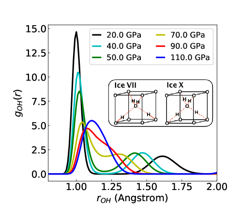
To demonstrate the methodology, we compute (a) the IR absorption spectrum of liquid water at standard temperature and pressure, and (b) the frequency dependent imaginary dielectric function in the high pressure transformation of ice VII to ice VII’, and from ice VII’ to ice X Hernandez and Caracas (2018). In ice VII there are 2 donor and 2 acceptor H-bonds per oxygen, as stipulated by the ice rule Bernal and Fowler (1933); Pauling (1935), and the water molecules are always well defined. In ice VII’ the hydrogens hop between two equivalent sites near each oxygen of an O-O bond, occasionally violating the ice rule. In ice X the hydrogens sit in the mid O-O bonds, the water molecules cannot be identified, and the system is better described in terms of O2- and H+ ions. This behavior is reflected in the O-H pair correlation functions in Fig. 1. For more sophisticated analyses and a phase diagram see e.g. Ref Hernandez and Caracas (2018). The polarization change accompanying the above transformations is seamlessly described by DW. The scheme should also work at higher temperature when ice X becomes superionic Millot et al. (2019), or at even higher temperature when the superionic crystal melts into an ionic liquid Rozsa et al. (2018). Similarly, the scheme should work for proton transfer events in water at standard conditions when neutral molecules interconvert with hydronium and hydroxide ion complexes (see e.g. Ref. Chen et al. (2018)).
In our implementation, DW is trained with valence only pseudopotential electronic structure calculations. In the laboratory frame, the positions of the atoms and of the WCs are and , respectively. We assume, for simplicity, that the WCs are only associated to one atomic species and consider water, in which there are 4 WCs per oxygen, as a concrete example 111Generalizations to more than one reference atom would be feasible to deal with situations in which the WC are shared among covalently bonded atoms of same electronegativity.. It is easy to select with a cutoff distance the 4 WCs with coordinates that are closer to the oxygen located at . Their centroid
| (1) |
is well defined even when water molecules cannot be identified. Our aim is to construct a vector function that gives if the positions of the atoms in the neighborhood of , defined by the radius , are known, i.e.:
| (2) |
Here is an oxygen atom but the atoms include oxygens and hydrogens. To ensure that preserves the translational, rotational, and permutational symmetry, we generalize the scheme for the Deep Potential (DP), the DNN representing the PES, introduced in Refs Zhang et al. (2018a, b).
First, we make a frame transformation to the primed coordinates, which preserve translational symmetry:
| (3) |
Then, we introduce a weight function equal to at short distance , and decaying smoothly to zero as approaches . Using , we describe the atomic coordinates with the 4-vector to enforce continuous evolution when atoms enter/exit the neighborhood.
Next, we enforce permutational invariance and rotational covariance by introducing two DNNs, an DNN and a DNN. The number of hidden layers and outputs is refined in the training procedure. The embedding DNN is the matrix with rows and columns optimized by training, which maps the set onto outputs.
The set of generalized coordinates in a neighborhood is represented by the matrix with rows and 4 columns. Multiplication of by gives the matrix with rows and 4 columns, whose generic element is:
| (4) |
Let be the matrix formed by the first (<) rows of . Multiplication of by , the transpose of , gives the matrix of dimension , called the feature matrix:
| (5) |
is the argument of the fitting DNN, a row matrix that converts the atomic coordinate information encoded in onto outputs, which are mapped onto the centroid upon multiplication with with the last three columns of :
| (6) |
Finally, is retrieved from using Eq. 3 and one obtains the desired representation of Eq. 2.
We notice that constructed in the way introduced above naturally preserves all the symmetry requirements. Translational symmetry is preserved by the adoption of a local frame and relative positions in Eq. 3. Permutational symmetry is preserved by the smooth sum over the neighboring atoms in Eq. 4. Finally, as shown in Eq. 4, the last three columns of () transform covariantly under rotation because transforms like . Then it is straightforward to verify that the elements of , and hence , are invariant under rotation. Therefore, in Eq. 6 transforms like , and is hence rotationally covariant. The values of , , and of the number of layers of the DNNs are chosen empirically based on performance. In the applications discussed in this paper we adopt =100 (of the same order of the number of atoms in a neighborhood), =6, and use a 3-layer representation for all the DNNs. The parameters of the embedding and fitting networks are determined by training, i.e., an optimization process that minimizes a loss function, here the mean square difference between the DW prediction and the training data. The Adam stochastic gradient descent method Kingma and Ba (2015) is adopted for the optimization. Generalization of this formalism to tensor properties (like the polarizability) is introduced in Ref. Sommers et al. (2020).
DW should be combined with a DNN for the PES to study the evolution of the polarization along MD trajectories. For consistency, the two networks should be trained with electronic structure data at the same level of theory, as in the applications below, which used DW and the DP representation of the PES Zhang et al. (2018a, b). Ab initio electronic structure data are expensive and efficient learning strategies are crucial. We used the iterative learning scheme of Ref. Zhang et al. (2019). In this approach, a DNN, initially trained with a limited pool of ab initio data, is used to explore inexpensively the configuration space. A small subset of the visited configurations is selected with a suitable error indicator and single shot ab initio calculations are performed at these configurations. Training with the new data improves the model for further exploration and selection, followed by new data acquisition and learning. The protocol is repeated until all the explored configurations are described with satisfactory accuracy. The error indicator exploits the highly non-linear dependence of the DNN models on the network parameters. As a consequence, different initializations of the parameters lead to different local minima in the landscape of the loss function, originating an ensemble of minimizing DNNs. The variance of the predictions within this ensemble is an intrinsic property of a DNN model and is often a reliable indicator of its accuracy Podryabinkin and Shapeev (2017); Zhang et al. (2018c). In our experience, good DNN models constructed with the above procedure require significantly less ab initio data in the target thermodynamic range than learning approaches based on independent AIMD sampling data.
In the following we report calculations on liquid water at STP and on ice undergoing pressure induced structural phase transitions. For liquid water at STP, we did not use the incremental data generation scheme, since the training data were available and accessible online from previous work Ko et al. (2019). For high-pressure ice, electronic structure data were not available, and we constructed DP and DW from scratch using the incremental learning procedure outlined above. Full details on the implementation, training, and validation of the models (DP and DW) are given in the Supplemental Material [SM]. The code for this work has been integrated into the open-source software package DeePMD-kit Wang et al. (2018) and we used the DP-GEN package Zhang et al. (2020) for the iterative scheme.
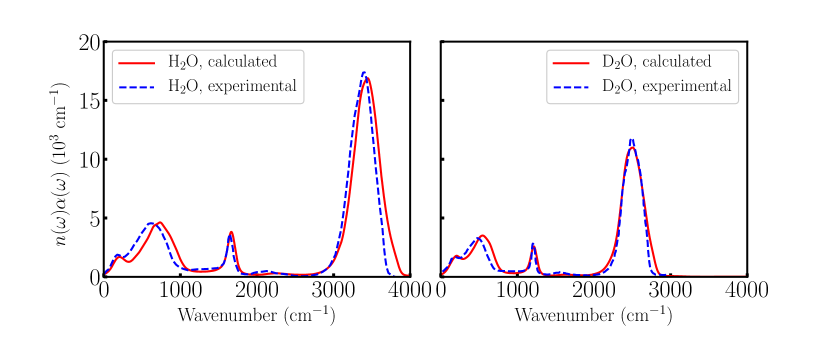
We use DFT at the hybrid functional level (PBE0 Adamo and Barone (1999)) with dispersion corrections Tkatchenko and Scheffler (2009) for STP water. Using DW and DP Zhang et al. (2018b) we calculate the IR absorption spectra of liquid H2O and D2O for a cell with 512 molecules under periodic boundary conditions. We use two microcanonical trajectories lasting 0.5 ns each, for H2O and D2O, at an average temperature of 300 K at the equilibrium density of the simulation. The frequency dependent absorption coefficient per unit length, , times the refractive index, , is given by the Fourier transform of the time correlation function of the time derivative of the cell polarization according to:
| (7) |
where is the volume, is the inverse temperature, and is Boltzmann’s constant. Fig. 2 shows that the calculated spectra are in good agreement with the corresponding experimental observations.
Similarly accurate IR spectra of liquid water can be obtained from representations of the PES Babin et al. (2013); Shank et al. (2009) and the dipole moment Liu et al. (2015) based on many-body molecular expansions. These powerful approaches are limited to molecular liquids and crystals. By contrast, our non-perturbative method works also for non-molecular systems, as we demonstrate by considering ice at T=300 K in the pressure range from 20 to 110 GPa, wherein structural phase transitions from ice VII to ice VII’ and to ice X occur. We adopted the PBE functional approximation of DFT as in Refs. Schwegler et al. (2008); Hernandez and Caracas (2018). We constructed DP/DW networks for ice in the temperature range from 240 to 330 K and pressure range from 20 to 120 GPa with the iterative learning approach set forth earlier in this paper. This procedure required a total of 2248 single shot DFT calculations with a 16 molecule cell and a total of 2400 single shot DFT calculations with a 128 molecule cell. For each cell size, the corresponding computational effort was less than the cost of a short (5 ps) AIMD trajectory.
We sampled the ice configurations at 300 K in the pressure range 20 - 110 GPa with constant pressure DPMD on a variable periodic cell with 128 water molecules, using a mild Nosé-Hoover thermostat Nosé (1984); Hoover (1985) with damping time of 5 ps, much longer than the vibrational periods, to control the temperature. Using DP+DW, we calculated according to Eq. 7 with a set of 0.5 ns long trajectories at various pressures. A direct AIMD study of the spectral changes in the closely related transformations from ice VIII (the proton ordered form of ice VII) to ice VII’ and to ice X, reported in a pioneering paper by Bernasconi et al. Bernasconi et al. (1998), used a small 16 molecule cell and 10 ps long trajectories.
Our results in Fig. 3 show a dramatic change with pressure of the product . We also report the same quantity obtained from reflectance measurements of pressurized ice in a diamond anvil cell Goncharov et al. (1996). Experimental data are not available for cm-1, and for 1800 cm2400 cm-1. The theoretical curves are displayed at approximately 10 GPa higher pressure than the experimental curves to empirically correct for the missing nuclear quantum effects in the simulation and the inaccuracy of the adopted functional approximation.
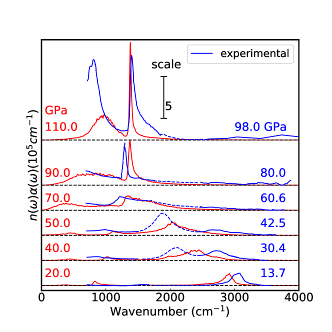
Taking into account the limitations of theory and experiment, the experimental trend is reproduced nicely by the DP+DW simulations. At the lowest pressures, molecular vibration features can be discerned, such as the H stretching band at about 3000 cm-1. These modes soften dramatically and broaden with pressure, indicating a progressive weakening of the covalent O-H bonds. In the simulation, the spectral changes are quite abrupt at 70 GPa, suggesting that this should be approximately the transition pressure to symmetric ice X. The same behavior is observed in experiment at 60 GPa. By further increasing the pressure, two strong features emerge, characteristic of ice X, that harden and sharpen with pressure. The higher frequency feature has dominant weight on H while the lower frequency feature has more O weight. Interestingly, there is no close correspondence between the IR spectrum and the power spectrum of atomic dynamics reported in the [SM], suggesting that extreme anharmonicity affects the IR spectrum, as pointed out in Ref. Bernasconi et al. (1998).
Quantum effects in the dynamics were ignored in our calculations. These effects are small but non-negligible in liquid water and should be more pronounced near the ice VII to X transition in view of the relatively large isotope effect on the transition pressure, which is 10 GPa higher for D2O than for H2O Goncharov et al. (1996), suggesting that the transition is facilitated by proton tunneling. The calculation of dynamic quantum correlation functions is a major challenge for statistical simulations. Quantum IR correlations have been calculated recently for liquid water using approximate methods like ring polymer Marsalek and Markland (2017) and centroid Marsalek and Markland (2017); Medders and Paesani (2015) MD, indicating that quantum corrections tend to red shift the classical spectral features. It would be extremely interesting to study how quantum corrections affect the dielectric properties in the ice VII, VII’, and X transition sequence. Further studies of these issues will be facilitated by methods like DPMD and DW, which improve significantly the statistical quality of ab initio simulations, as they are orders of magnitude faster than DFT methods and scale linearly with system size. Quantitative cost comparisons between direct AIMD and DP/DW simulations are reported in Figs. S2 and S3 in the [SM].
In summary, DW is a useful tool to parametrize the dependence of the polarization on the atomic environment. The approach can be naturally extended Sommers et al. (2020) to the environmental dependence of the polarizability tensor ( and are Cartesian components of the polarization and of the electric field), allowing us to compute Raman Wan et al. (2013); Sommers et al. (2020) and sum frequency generation spectra Mukamel (1998); Nagata and Mukamel (2010). Access to the concerted evolution of atomic coordinates and polarization in simulations of large systems over long time scales should also open the way to studies of ferroelectric phase transitions with MD simulations of ab initio quality, rather than relying on effective Hamiltonian models Resta and Vanderbilt (2007); Srinivasan et al. (2003); Vanderbilt and Zhong (1998). Finally, related symmetry preserving DNN schemes have been considered in Refs. Zaheer et al. (2017); Battaglia et al. (2018); Esteves et al. (2018); Han et al. (2019) and we defer to future work a discussion of the mathematical and machine learning aspects of the DP/DW models.
Acknowledgements.
The work of L. Z., X. W., W. E, and R.C. was conducted at the Center “Chemistry in Solution and at Interfaces” (CSI) funded by the DOE Award DE-SC001934. The work of L. Z and W. E was partially supported by a gift from iFlytek to Princeton University and by ONR grant N00014-13-1-0338. The work of H.W. was supported by the NSFC under grant 11871110, and the National Key Research and Development Program of China under grants 2016YFB0201200 and 2016YFB0201203. We used resources of the National Energy Research Scientific Computing Center (DoE Contract No. DE-AC02-05cH11231). We are also grateful for computing time at the Terascale Infrastructure for Groundbreaking Research in Science and Engineering (TIGRESS) of Princeton University.References
- Behler and Parrinello (2007) J. Behler and M. Parrinello, Physical Review Letters 98, 146401 (2007).
- Bartók et al. (2010) A. P. Bartók, M. C. Payne, R. Kondor, and G. Csányi, Physical Review Letters 104, 136403 (2010).
- Rupp et al. (2012) M. Rupp, A. Tkatchenko, K.-R. Müller, and O. A. VonLilienfeld, Physical Review Letters 108, 058301 (2012).
- Montavon et al. (2013) G. Montavon, M. Rupp, V. Gobre, A. Vazquez-Mayagoitia, K. Hansen, A. Tkatchenko, K.-R. Müller, and O. A. Von Lilienfeld, New Journal of Physics 15, 095003 (2013).
- Botu et al. (2016) V. Botu, R. Batra, J. Chapman, and R. Ramprasad, The Journal of Physical Chemistry C 121, 511 (2016).
- Chmiela et al. (2017) S. Chmiela, A. Tkatchenko, H. E. Sauceda, I. Poltavsky, K. T. Schütt, and K.-R. Müller, Science Advances 3, e1603015 (2017).
- Schütt et al. (2017) K. Schütt, P.-J. Kindermans, H. E. S. Felix, S. Chmiela, A. Tkatchenko, and K.-R. Müller, in Advances in Neural Information Processing Systems (2017) pp. 992–1002.
- Smith et al. (2017) J. S. Smith, O. Isayev, and A. E. Roitberg, Chemical Science 8, 3192 (2017).
- Han et al. (2018) J. Han, L. Zhang, R. Car, and W. E, Communications in Computational Physics 23, 629 (2018).
- Zhang et al. (2018a) L. Zhang, J. Han, H. Wang, R. Car, and W. E, Physical Review Letters 120, 143001 (2018a).
- Zhang et al. (2018b) L. Zhang, J. Han, H. Wang, W. Saidi, R. Car, and W. E, in Advances in Neural Information Processing Systems 31, edited by S. Bengio, H. Wallach, H. Larochelle, K. Grauman, N. Cesa-Bianchi, and R. Garnett (Curran Associates, Inc., 2018) pp. 4441–4451.
- Kohn and Sham (1965) W. Kohn and L. J. Sham, Physical Review 140, A1133 (1965).
- Car and Parrinello (1985) R. Car and M. Parrinello, Physical Review Letters 55, 2471 (1985).
- Marx and Hutter (2009) D. Marx and J. Hutter, Ab initio molecular dynamics: basic theory and advanced methods (Cambridge University Press, 2009).
- Bonati and Parrinello (2018) L. Bonati and M. Parrinello, Physical Review Letters 121, 265701 (2018).
- Gastegger et al. (2017) M. Gastegger, J. Behler, and P. Marquetand, Chemical Science 8, 6924 (2017).
- Grisafi et al. (2018a) A. Grisafi, D. M. Wilkins, G. Csányi, and M. Ceriotti, Physical Review Letters 120, 036002 (2018a).
- Grisafi et al. (2018b) A. Grisafi, A. Fabrizio, B. Meyer, D. M. Wilkins, C. Corminboeuf, and M. Ceriotti, ACS Central Science 5, 57 (2018b).
- Wilkins et al. (2019) D. M. Wilkins, A. Grisafi, Y. Yang, K. U. Lao, R. A. DiStasio, and M. Ceriotti, Proceedings of the National Academy of Sciences , 201816132 (2019).
- Chandrasekaran et al. (2019) A. Chandrasekaran, D. Kamal, R. Batra, C. Kim, L. Chen, and R. Ramprasad, NPJ Computational Materials 5, 22 (2019).
- Zepeda-Núñez et al. (2019) L. Zepeda-Núñez, Y. Chen, J. Zhang, W. Jia, L. Zhang, and L. Lin, arXiv preprint arXiv:1912.00775 (2019).
- Raimbault et al. (2019) N. Raimbault, A. Grisafi, M. Ceriotti, and M. Rossi, New Journal of Physics 21, 105001 (2019).
- Kapil et al. (2019) V. Kapil, D. M. Wilkins, J. Lan, and M. Ceriotti, arXiv preprint arXiv:1912.03189 (2019).
- Sharma et al. (2005) M. Sharma, R. Resta, and R. Car, Physical Review Letters 95, 187401 (2005).
- Putrino et al. (2000) A. Putrino, D. Sebastiani, and M. Parrinello, The Journal of Chemical Physics 113, 7102 (2000).
- Wan et al. (2013) Q. Wan, L. Spanu, G. A. Galli, and F. Gygi, Journal of Chemical Theory and Computation 9, 4124 (2013).
- Wan and Galli (2015) Q. Wan and G. Galli, Physical Review Letters 115, 246404 (2015).
- Rozsa et al. (2018) V. Rozsa, D. Pan, F. Giberti, and G. Galli, Proceedings of the National Academy of Sciences 115, 6952 (2018).
- Sun et al. (2015) J. Sun, B. K. Clark, S. Torquato, and R. Car, Nature communications 6, 8156 (2015).
- Wood and Marzari (2006) B. C. Wood and N. Marzari, Physical review letters 97, 166401 (2006).
- Schwegler et al. (2008) E. Schwegler, M. Sharma, F. Gygi, and G. Galli, Proceedings of the National Academy of Sciences 105, 14779 (2008).
- Srinivasan et al. (2003) V. Srinivasan, R. Gebauer, R. Resta, and R. Car, in AIP Conference Proceedings, Vol. 677 (AIP, 2003) pp. 168–175.
- Fluri et al. (2017) A. Fluri, A. Marcolongo, V. Roddatis, A. Wokaun, D. Pergolesi, N. Marzari, and T. Lippert, Advanced Science 4, 1700467 (2017).
- Liu et al. (2015) H. Liu, Y. Wang, and J. M. Bowman, The Journal of chemical physics 142, 194502 (2015).
- Marzari and Vanderbilt (1997) N. Marzari and D. Vanderbilt, Physical Review B 56, 12847 (1997).
- Marzari et al. (2012) N. Marzari, A. A. Mostofi, J. R. Yates, I. Souza, and D. Vanderbilt, Reviews of Modern Physics 84, 1419 (2012).
- Resta (1994) R. Resta, Reviews of Modern Physics 66, 899 (1994).
- Kohn (1996) W. Kohn, Physical Review Letters 76, 3168 (1996).
- Prodan and Kohn (2005) E. Prodan and W. Kohn, Proceedings of the National Academy of Sciences 102, 11635 (2005).
- Hernandez and Caracas (2018) J.-A. Hernandez and R. Caracas, The Journal of Chemical Physics 148, 214501 (2018).
- Bernal and Fowler (1933) J. D. Bernal and R. H. Fowler, The Journal of Chemical Physics 1, 515 (1933).
- Pauling (1935) L. Pauling, Journal of the American Chemical Society 57, 2680 (1935).
- Millot et al. (2019) M. Millot, F. Coppari, J. R. Rygg, A. C. Barrios, S. Hamel, D. C. Swift, and J. H. Eggert, Nature 569, 251 (2019).
- Chen et al. (2018) M. Chen, L. Zheng, B. Santra, H.-Y. Ko, R. A. DiStasio Jr, M. L. Klein, R. Car, and X. Wu, Nature chemistry 10, 413 (2018).
- Kingma and Ba (2015) D. Kingma and J. Ba, in Proceedings of the International Conference on Learning Representations (ICLR) (2015).
- Sommers et al. (2020) G. M. Sommers, M. F. Calegari Andrade, L. Zhang, H. Wang, and R. Car, Phys. Chem. Chem. Phys. 22, 10592 (2020).
- Zhang et al. (2019) L. Zhang, D.-Y. Lin, H. Wang, R. Car, and W. E, Physical Review Materials 3, 023804 (2019).
- Podryabinkin and Shapeev (2017) E. V. Podryabinkin and A. V. Shapeev, Computational Materials Science 140, 171 (2017).
- Zhang et al. (2018c) L. Zhang, H. Wang, and W. E, The Journal of Chemical Physics 148, 124113 (2018c).
- Ko et al. (2019) H.-Y. Ko, L. Zhang, B. Santra, H. Wang, W. E, R. A. DiStasio Jr, and R. Car, Molecular Physics , 1 (2019).
- Wang et al. (2018) H. Wang, L. Zhang, J. Han, and W. E, Computer Physics Communications 228, 178 (2018).
- Zhang et al. (2020) Y. Zhang, H. Wang, W. Chen, J. Zeng, L. Zhang, H. Wang, and W. E, Computer Physics Communications , 107206 (2020).
- Bertie and Lan (1996) J. E. Bertie and Z. Lan, Applied Spectroscopy 50, 1047 (1996).
- Bertie et al. (1989) J. E. Bertie, M. K. Ahmed, and H. H. Eysel, The Journal of Physical Chemistry 93, 2210 (1989).
- Adamo and Barone (1999) C. Adamo and V. Barone, The Journal of Chemical Physics 110, 6158 (1999).
- Tkatchenko and Scheffler (2009) A. Tkatchenko and M. Scheffler, Physical Review Letters 102, 073005 (2009).
- Babin et al. (2013) V. Babin, C. Leforestier, and F. Paesani, Journal of Chemical Theory and Computation 9, 5395 (2013).
- Shank et al. (2009) A. Shank, Y. Wang, A. Kaledin, B. J. Braams, and J. M. Bowman, The Journal of Chemical Physics 130, 144314 (2009).
- Nosé (1984) S. Nosé, The Journal of Chemical Physics 81, 511 (1984).
- Hoover (1985) W. G. Hoover, Physical review A 31, 1695 (1985).
- Bernasconi et al. (1998) M. Bernasconi, P. Silvestrelli, and M. Parrinello, Physical Review Letters 81, 1235 (1998).
- Goncharov et al. (1996) A. Goncharov, V. Struzhkin, M. Somayazulu, R. Hemley, and H. Mao, Science 273, 218 (1996).
- Marsalek and Markland (2017) O. Marsalek and T. E. Markland, The Journal of Physical Chemistry Letters 8, 1545 (2017).
- Medders and Paesani (2015) G. R. Medders and F. Paesani, Journal of Chemical Theory and Computation 11, 1145 (2015).
- Mukamel (1998) S. Mukamel, Principles of nonlinear optical spectroscopy, Vol. 41 (1998) pp. 591–592.
- Nagata and Mukamel (2010) Y. Nagata and S. Mukamel, Journal of the American Chemical Society 132, 6434 (2010).
- Resta and Vanderbilt (2007) R. Resta and D. Vanderbilt, in Physics of Ferroelectrics (Springer, 2007) pp. 31–68.
- Vanderbilt and Zhong (1998) D. Vanderbilt and W. Zhong, Ferroelectrics 206, 181 (1998).
- Zaheer et al. (2017) M. Zaheer, S. Kottur, S. Ravanbakhsh, B. Poczos, R. R. Salakhutdinov, and A. J. Smola, in Advances in Neural Information Processing Systems 30, edited by I. Guyon, U. V. Luxburg, S. Bengio, H. Wallach, R. Fergus, S. Vishwanathan, and R. Garnett (Curran Associates, Inc., 2017) pp. 3391–3401.
- Battaglia et al. (2018) P. W. Battaglia, J. B. Hamrick, V. Bapst, A. Sanchez-Gonzalez, V. Zambaldi, M. Malinowski, A. Tacchetti, D. Raposo, A. Santoro, R. Faulkner, et al., arXiv preprint arXiv:1806.01261 (2018).
- Esteves et al. (2018) C. Esteves, C. Allen-Blanchette, A. Makadia, and K. Daniilidis, in Proceedings of the European Conference on Computer Vision (ECCV) (2018) pp. 52–68.
- Han et al. (2019) J. Han, Y. Li, L. Lin, J. Lu, J. Zhang, and L. Zhang, arXiv preprint arXiv:1912.01765 (2019).