Importance of multicranked configuration mixing for angular-momentum-projection calculations:
Study of superdeformed rotational bands in ¹⁵²Dy and ¹⁹⁴Hg

Abstract

Recently we have investigated an effective method of multicranked configuration-mixing for angular-momentum-projection calculation, where several cranked mean-field states are coupled after projection: The basic idea was originally proposed by Peierls and Thouless more than fifty years ago. With this method a good description of the rotational band has been achieved in a fully microscopic manner. In the present work, we apply the method to the high-spin superdeformed band, for which long rotational sequence is observed, and study how the good description is obtained for the rotational spectrum as well as the ${\cal J}^{(1)}$ and ${\cal J}^{(2)}$ moments of inertia as functions of angular momentum. The Gogny D1S force is employed as an effective interaction, and the yrast superdeformed bands in ¹⁵²Dy and ¹⁹⁴Hg are taken as typical examples in the $A\approx 150$ and $A\approx 190$ regions, respectively. The effect of pairing correlations is examined by the variation after particle-number projection approach to understand the different behaviors of ${\cal J}^{(2)}$ moments of inertia observed in these two nuclei. The particle-number projection on top of the angular-momentum projection has been performed for the first time with the multicranked configuration-mixing.

I Introduction

Collective motion in atomic nuclei has been an interesting subject in nuclear structure physics BM75 ; RS80 . The rotational motion is a typical collective motion and exhibits many interesting phenomena especially at high-spin states, see e.g. Refs. VDS83 ; GHH86 ; Fra01 ; WP01 ; SW05 ; Fra18 . Recently, we have developed a theoretical framework for describing the high-spin rotational band in a fully microscopic manner by employing the technique of angular-momentum projection from the selfconsistent mean-field states STS15 . We called it “angular-momentum-projected multicranked configuration-mixing”, where several selfconsistently cranked mean-field states are quantum-mechanically coupled after projection. It has been shown that good agreement of the spectra and the kinematic moments of inertia, ${\cal J}^{(1)}$, is obtained for the ground-state rotational bands in rare earth nuclei without any adjustable parameters STS16 . In contrast to the projected shell-model approach, where the angular-momentum projection method is successfully applied, see e.g. Refs. HS95 ; Sun16 ; SBD16 , the number of mean-field states coupled after projection is relatively small in our approach, where they are obtained selfconsistently within the cranking procedure.

Generally, calculation of the mass parameter is crucial for the appropriate description of nuclear collective motion. It has been well-known that the generator coordinate method (GCM) with only collective coordinates does not give proper mass parameter, see e.g. Sec. ⁢11.4.5 of Ref. RS80 for the instructive argument especially for the center-of-mass motion. The angular-momentum projection procedure is a special case of the GCM for the collective rotational motion with the Euler angles as collective coordinates. In order to obtain the proper mass, Peierls and Thouless proposed to superpose not only wave functions with different coordinates but also those with different velocities (or momenta) PT62 , which incorporates time-odd components into the wave function; the correct total mass appears for the center-of-mass motion as a result of the boost because of the Galilean invariance. In fact the time-odd components are generally important for mass parameters, and we have investigated a procedure to take them into account, which we call “infinitesimal cranking”, and successfully applied it to the collective $\gamma$-vibration in Ref. TS16 .

The basic idea of the framework of multicranked configuration-mixing STS15 is nothing else but the one proposed by Peierls and Thouless for the rotational motion PT62 , i.e., the total wave function is calculated as

$$|\Psi^{I}_{M,\alpha}\rangle=\int d\omega_{\rm rot}\sum_{K}g^{I}_{K,\alpha}(\omega_{\rm rot})\,\hat{P}^{I}_{MK}|\Phi(\omega_{\rm rot})\rangle,$$ (1)

where the operator $\hat{P}^{I}_{MK}$ is the angular-momentum projector, and $g^{I}_{K,\alpha}(\omega_{\rm rot})$ is the amplitude of superposition. Here the cranked mean-field state, $|\Phi(\omega_{\rm rot})\rangle$, with the rotational frequency (angular velocity), $\omega_{\rm rot}$, is determined by the selfconsistent cranking procedure RS80 . There is no principle like the Galilean invariance for the rotational motion, and the configuration-mixing with respect to the cranking frequency in Eq. (1) should be evaluated numerically, as it will be discussed in more detail below in Sec. II. The same method has been also applied recently for the GCM calculation with respect to the $(\beta,\gamma)$ collective coordinates in Ref. BRE15 .

In the present work, we apply the framework to the superdeformed rotational band, which is one of the most striking rotational motions in nuclei, see e.g. Refs. SDtwin ; SDrevA ; SDrevB ; SDrevC . With this application we would like to demonstrate the importance of multicranked configuration-mixing especially for high-spin states; proper description of the moment of inertia for superdeformed states cannot be obtained by the angular-momentum-projection calculation from a single mean-field state. The superdeformed band is best suited for this investigation because long rotational sequences have been measured without any quasiparticle-alignments in many cases. Moreover, the influence of pairing correlations is relatively small on the moments of inertia of the superdeformed states; for the normal deformed states studied in the previous work STS16 the reduction of moments of inertia due to the static pairing correlations is very large, the reduction factor being 1/2 to 1/3 as is well-known, and it is not so easy to identify the importance of multicranked configuration-mixing.

The yrast superdeformed bands of two even-even nuclei, ¹⁵²Dy and ¹⁹⁴Hg, are selected as representative examples in the $A\approx 150$ and $A\approx 190$ regions. It has been known that the behaviors of the dynamic moments of inertia BM81 , ${\cal J}^{(2)}$, are different for the superdeformed bands in the two mass regions. The reason for selecting these two nuclei is that the linking transitions were measured and the spin assignments were given. Therefore we can study both ${\cal J}^{(1)}$ and ${\cal J}^{(2)}$ moments of inertia as functions of angular momentum. Another purpose of the present paper is to look for the main reason of the difference in these two mass regions; the effect of pairing correlations is studied for this purpose employing the cranked mean-field states obtained by the variation after number projection approach. Then the particle-number projection as well as the angular-momentum projection have been carried out for the first time in this type of multicranked configuration-mixing calculations.

The paper is organized as follows. We briefly explain the basic formulation of the actual procedure in Sec. II. The results of calculation are presented in Sec. III, where the importance of multicranked configuration-mixing is discussed for typical examples of the yrast superdeformed bands in the ¹⁵²Dy and ¹⁹⁴Hg nuclei. A part of the results of moments of inertia for ¹⁵²Dy was already presented in Ref. STS15 ; the process of configuration-mixing leading to the results is investigated in more detail in comparison with another nucleus ¹⁹⁴Hg in this section. Sec. IV is devoted to conclusion.

II Theoretical framework

II.1 Multicranked configuration-mixing

Practically we discretize the continuous cranking frequency $\omega_{\rm rot}$ in Eq. (1), as {$\omega^{(n)}_{\rm rot}$; $n=1,2,\cdots,n_{\rm max}$},

$$|\Psi^{I}_{M,\alpha}\rangle=\sum_{n=1}^{n_{\rm max}}\sum_{K}g^{I}_{Kn,\alpha}\,\hat{P}^{I}_{MK}|\Phi(\omega_{\rm rot}^{(n)})\rangle,$$ (2)

and obtain the configuration-mixing amplitudes, $g^{I}_{Kn,\alpha}\equiv g^{I}_{K,\alpha}(\omega_{\rm rot}^{(n)})$, by solving the so-called Hill-Wheeler equation, see e.g. Ref. RS80 ,

$$\sum_{K^{\prime}n^{\prime}}{\cal H}^{I}_{Kn,K^{\prime}n^{\prime}}\ g^{I}_{K^{\prime}n^{\prime},\alpha}=E^{I}_{\alpha}\,\sum_{K^{\prime}n^{\prime}}{\cal N}^{I}_{Kn,K^{\prime}n^{\prime}}\ g^{I}_{K^{\prime}n^{\prime},\alpha},$$ (3)

where the Hamiltonian and norm kernels are defined by

$$\left\{\begin{array}[]{c}{\cal H}^{I}_{Kn,K^{\prime}n^{\prime}}\\ {\cal N}^{I}_{Kn,K^{\prime}n^{\prime}}\end{array}\right\}=\langle\Phi(\omega_{\rm rot}^{(n)})|\left\{\begin{array}[]{c}H\\ 1\end{array}\right\}\hat{P}_{KK^{\prime}}^{I}|\Phi(\omega_{\rm rot}^{(n^{\prime})})\rangle.$$ (4)

If the particle-number projection is performed on top of the angular-momentum projection (see below), the wave function in Eqs. (1), (2) and (4) is replaced as

$$\hat{P}^{I}_{MK}|\Phi(\omega_{\rm rot})\rangle\rightarrow\hat{P}^{I}_{MK}\,\hat{P}^{N_{0}}\hat{P}^{Z_{0}}|\Phi(\omega_{\rm rot})\rangle,$$ (5)

where $\hat{P}^{N_{0}}$ and $\hat{P}^{Z_{0}}$ are the neutron- and proton-number projectors fixing the neutron and proton numbers to the desired values $N_{0}$ and $Z_{0}$, respectively. If the particle-number projection is not performed, the number conservation is treated approximately by replacing $H\rightarrow H-\lambda_{\nu}(N-N_{0})-\lambda_{\pi}(Z-Z_{0})$. As for the neutron and proton chemical potentials $\lambda_{\nu}$ and $\lambda_{\pi}$ we use those of the first state $|\Phi(\omega_{\rm rot}^{(1)})\rangle$.

We have recently developed an efficient method for the angular-momentum-projection and the configuration-mixing calculation TS12 . This method is fully utilized also in the present work. More details of our theoretical framework can be found in Refs. TS12 ; STS15 . As for an effective interaction in the Hamiltonian $H$, we employ the Gogny force DeGo80 with the so-called D1S parametrization D1S as in our previous works STS15 ; TS16 ; STS16 ; therefore, there is no adjustable parameter in the Hamiltonian. This interaction has been utilized in many applications of the Hartree-Fock-Bogolyubov (HFB) calculation and various theoretical methods beyond it, see e.g. Ref. Egido16 .

II.2 Determination of the mean-field states

The mean-field state, $|\Phi(\omega_{\rm rot})\rangle$ with $\omega_{\rm rot}=\omega^{(n)}_{\rm rot}$, is determined by the cranked HFB procedure with the routhian (cranked Hamiltonian), $H-\omega_{\rm rot}J_{y}$, i.e., by the variation,

$$\delta\langle\Phi(\omega_{\rm rot})|H-\omega_{\rm rot}J_{y}|\Phi(\omega_{\rm rot})\rangle=0.$$ (6)

The selfconsistent mean-fields of the superdeformed nuclei studied in the present work are axially-deformed in a good approximation even at highest frequencies. We choose the $z$ axis as the (approximate) symmetry axis and the $y$ axis as a cranking axis, as it can be seen in Eq. (6). Namely, we consider the one-dimensional cranking in the present work. The full three-dimensional cranking KO81 , or the tilted-axis cranking Fra93 ; Fra00 , is necessary when deformation of the mean-field strongly breaks the axial symmetry. The infinitesimal cranking for such a case was worked out in Ref. TS16 .

It should be mentioned that with this cranked HFB procedure the pairing correlation vanishes suddenly at some critical frequency. However, for the finite system like a nucleus, the pairing phase-transition takes place gradually and the effect of pairing fluctuations plays non-negligible roles near and after the critical frequency, see e.g. Ref. pairRMP . In this reference, the pairing fluctuations calculated by the random-phase approximation (RPA) method have been investigated at the high-spin states, and shown to systematically improve the agreement of the routhians and alignments with experimental data; see also Refs. SDB00 ; ADF00 .

The same methodology has been successfully applied to investigate the ${\cal J}^{(1)}$ and ${\cal J}^{(2)}$ moments of inertia of the superdeformed bands in the $A\approx 150$ region SVB90 , where the Nilsson-Strutinsky method with the schematic monopole pairing interaction has been utilized. It is, however, noted that the angular-momentum projection from the RPA-correlated state is difficult to perform, though not impossible; see e.g. Ref. FR85 . An alternative method to incorporate the pairing fluctuations into the mean-field is the method of variation after (particle-)number projection (VANP), see e.g. Ref. RS80 . The effect of pairing fluctuations calculated by the RPA and the VANP methods has been compared in Ref. SB90 and it has been confirmed that the two methods give very similar results for observable quantities, see also the discussion in Ref. YRS90 . In Ref. NWJ89 the effect of pairing correlation has been studied for the superdeformed bands in the $A\approx 150$ region using the number projection method, where the Woods-Saxon-Strutinsky calculation with the schematic monopole pairing interaction has been employed, and the pairing-gap parameter has been taken as a variational parameter. Similar improvement over the simple mean-field approximation has been obtained in these Refs. SVB90 ; NWJ89 .

In relation to these developments, it may be worthwhile mentioning that microscopic mean-field calculations employing the Skyrme force with various density-dependent zero-range pairing interactions have been performed for superdeformed nuclei in the $A\approx 190$ region THB95 and in the $A\approx 150$ region BFH96 with good agreements. The same line of investigation but by using the Gogny force has been reported, see e.g. Refs. GDB94 ; VER00 ; in the latter reference VER00 the effect of approximate number projection on the superdeformed states has been also investigated. The relativistic mean-field method has been also successfully applied to the high-spin superdeformed rotational bands in the $A\approx 140-150$ mass region, see e.g. Ref. AKR96 .

To incorporate the effect of pairing fluctuations, we also present the results of calculation, where the mean-field state, $|\Phi(\omega_{\rm rot})\rangle$, is determined by the VANP method, instead of the cranked HFB method in Eq. (6), i.e., by the variation,

$$\delta\frac{\langle\Phi(\omega_{\rm rot})|(H-\omega_{\rm rot}J_{y})\hat{P}^{N_{0}}\hat{P}^{Z_{0}}|\Phi(\omega_{\rm rot})\rangle}{\langle\Phi(\omega_{\rm rot})|\hat{P}^{N_{0}}\hat{P}^{Z_{0}}|\Phi(\omega_{\rm rot})\rangle}=0.$$ (7)

In the present work the Gogny D1S effective interaction is used and the variation with respect to the full-HFB amplitudes should be performed. One of the common method is the gradient method, see e.g. Ref. RS80 , but it takes a lot of iterations to achieve precise convergence. An efficient method by utilizing diagonalization of the number-projected quasiparticle Hamiltonian has been developed in Ref. SR00 ; we make its full use to obtain the cranked VANP mean-field state in Eq. (7). With the VANP method, the particle-number projection should be performed on top of the angular-momentum projection for multicranked configuration-mixing, see Eq. (5).

Since the deformation is axially-symmetric in a good approximation, we define the $\lambda$-pole deformation parameter of the calculated mean-field defined as usual by IMY02

$$\beta_{\lambda}\equiv\frac{4\pi}{3}\,\frac{\displaystyle\biggl{\langle}\sum_{i=1}^{A}(r^{\lambda}Y_{\lambda 0})_{i}\biggr{\rangle}}{A\,\bar{R}^{\lambda}},\qquad\mbox{with}\quad\bar{R}=\sqrt{\frac{5}{3A}\biggl{\langle}\sum_{i=1}^{A}r_{i}^{2}\biggr{\rangle}},$$ (8)

and the average pairing gap by BRRM00

$$\Delta\equiv\frac{\displaystyle-\sum_{a>b}\Delta_{ab}\kappa^{*}_{ab}}{\displaystyle\sum_{a>b}\kappa^{*}_{ab}},\qquad\mbox{with}\quad\Delta_{ab}=\sum_{c>d}\bar{v}_{ab,cd}\,\kappa_{cd},$$ (9)

where the quantity $\kappa_{ab}$ is the abnormal density matrix (the pairing tensor) and $\Delta_{ab}$ is the matrix element of the pairing potential with the anti-symmetrized matrix element $\bar{v}_{ab,cd}$ of the general two-body interaction, see e.g. Ref. RS80 .

II.3 Two moments of inertia

Although it is a textbook matter, we here summarize the expressions of the two moments of inertia, that is, the kinematic and dynamic ones BM81 , for completeness. For the spectrum of simple one-dimensional rotation $E(I)$, the rotational frequency $\omega_{\rm rot}$ is defined by

$$\omega_{\rm rot}=\frac{dE}{dI},$$ (10)

which determine the $\omega_{\rm rot}-I$ relation $I(\omega_{\rm rot})$. Then, the routhian, i.e., the energy in the rotating frame $E^{\prime}(\omega_{\rm rot})$, is given by the Legendre transformation,

$$E^{\prime}(\omega_{\rm rot})=E\bigl{(}I(\omega_{\rm rot})\bigr{)}-\omega_{\rm rot}I(\omega_{\rm rot}).$$ (11)

With these definitions, the two moments of inertia, ${\cal J}^{(2)}$ and ${\cal J}^{(1)}$, are expressed in various equivalent ways by

$${\cal J}^{(1)}=I\left(\frac{dE}{dI}\right)^{-1}=\frac{I}{\omega_{\rm rot}}=-\frac{1}{\omega_{\rm rot}}\frac{dE^{\prime}}{d\omega_{\rm rot}},$$ (12)

$${\cal J}^{(2)}=\left(\frac{d^{2}E}{dI^{2}}\right)^{-1}=\frac{dI}{d\omega_{\rm rot}}=-\frac{d^{2}E^{\prime}}{d\omega^{2}_{\rm rot}}.$$ (13)

III Results of calculation

III.1 Details of calculation

In the mean-field calculation such as the cranked HFB or VANP and the subsequent angular-momentum-projection calculation, the isotropic harmonic oscillator basis expansion is employed, where all the basis states with the oscillator quantum numbers $(n_{x},n_{y},n_{z})$ satisfying $n_{x}+n_{y}+n_{z}\leq N_{\rm osc}^{\rm max}=12$ are retained. The value of canonical basis cut-off factor to define the effective quasiparticle space is taken to be $10^{-6}$ in the same way as in Ref. TS12 . The value of norm cut-off factor for solving the Hill-Wheeler equation, see e.g. Ref. RS80 , is chosen to be $10^{-12}\sim 10^{-9}$ in order to obtain as continuous rotational bands as possible STS15 ; STS16 .

The maximum values of the angular-momentum and its projection to the (approximate) symmetry axis are taken to be $I_{\rm max}=62$ and $K_{\rm max}=22$ for ¹⁵²Dy, and $I_{\rm max}=52$ and $K_{\rm max}=22$ for ¹⁹⁴Hg. Note that the cranking procedure with high rotational frequency causes considerable $K$-mixing although the deformation is approximately axially-symmetric, and, therefore, $K_{\rm max}$ should not be very small. We have confirmed that the selected values above are enough for the present calculation. As for the numbers of integration-mesh points for the Euler angles ($\alpha,\beta,\gamma$) in the calculation of angular-momentum projector, rather large values especially for the $\beta$ integration are necessary to obtain precise energy spectrum up to high-spin states like $I\approx 60$. We have used $N_{\beta}=130$ and $N_{\alpha}=N_{\gamma}=60$ after confirming accuracy of the results. To perform the VANP calculation in Eq. (7) the particle-number projector should be applied, for which the number of integration-mesh points for the gauge angle $\phi$ has been taken to be $N_{\phi}=7$.

As for the number of mean-field states of multicranked configuration-mixing in Eq. (2), we use $n_{\rm max}=4$ in the present work. A larger value of $n_{\rm max}$ is preferable, but the numerical efforts to perform the angular-momentum projection are too much with relatively large numbers of integration-mesh points for the Euler angles being employed in the present calculation; note that the numerical cost increases in proportion to $n^{2}_{\rm max}$. With the mean-field states obtained by the VANP method, we carry out the particle-number projection on top of the angular-momentum projection as is explained in Sec. II.2; then the numerical cost is $N_{\phi}\,(=7)$ times larger.

The discretized points of the rotational frequency, $\omega^{(n)}_{\rm rot}$ ($n=1,\cdots,n_{\rm max}=4$), can be chosen rather arbitrarily; in Ref. STS15 it is discussed that the final results of configuration-mixing do not depend on this choice when enough number of points are employed. We select the first and last points, $\omega^{(1)}_{\rm rot}$ and $\omega^{(4)}_{\rm rot}$, and other points are determined to form the equidistant-mesh. Some trial-and-error has been done to obtain the smooth rotational band, which is necessary to calculate kinematic and dynamic moments of inertia. In the following, we mainly discuss the ${\cal J}^{(2)}$ moment of inertia evaluated with the discrete ${\mit\Delta}I=\pm 2$ rotational spectrum, $E(I)$,

$${\cal J}^{(2)}(I)=\frac{4\hbar^{2}}{E(I+2)+E(I-2)-2E(I)}=\frac{4\hbar^{2}}{E_{\gamma}(I+1)-E_{\gamma}(I-1)},$$ (14)

for the experimental data and for the calculated results of projection, where $E_{\gamma}(I)\equiv E(I+1)-E(I-1)$ is the $\gamma$-ray energy of the $I+1\rightarrow I-1$ transition. Note that these quantities can be evaluated only with the $\gamma$-ray energies without the spin-assignment, which is often missing for superdeformed rotational bands. We also discuss the ${\cal J}^{(1)}$ moment of inertia,

$${\cal J}^{(1)}(I)=\frac{(2I+1)\hbar^{2}}{E(I+1)-E(I-1)}=\frac{(2I+1)\hbar^{2}}{E_{\gamma}(I)},$$ (15)

which requires the spin-assignment to calculate. The ${\cal J}^{(2)}$ moment of inertia calculated within the cranked HFB approximation,

$${\cal J}^{(2)}(\omega_{\rm rot})=\frac{d}{d\omega_{\rm rot}}\langle\Phi(\omega_{\rm rot})|J_{y}|\Phi(\omega_{\rm rot})\rangle,$$ (16)

as a function of semiclassical spin value defined by

$$I(\omega_{\rm rot})\equiv\langle\Phi(\omega_{\rm rot})|J_{y}|\Phi(\omega_{\rm rot})\rangle-{\frac{1}{2}}\hbar,$$ (17)

or within the cranked VANP approximation,

$${\cal J}^{(2)}(\omega_{\rm rot})=\frac{d}{d\omega_{\rm rot}}\frac{\langle\Phi(\omega_{\rm rot})|J_{y}\,\hat{P}^{N_{0}}\hat{P}^{Z_{0}}|\Phi(\omega_{\rm rot})\rangle}{\langle\Phi(\omega_{\rm rot})|\hat{P}^{N_{0}}\hat{P}^{Z_{0}}|\Phi(\omega_{\rm rot})\rangle},$$ (18)

as a function of

$$I(\omega_{\rm rot})\equiv\frac{\langle\Phi(\omega_{\rm rot})|J_{y}\,\hat{P}^{N_{0}}\hat{P}^{Z_{0}}|\Phi(\omega_{\rm rot})\rangle}{\langle\Phi(\omega_{\rm rot})|\hat{P}^{N_{0}}\hat{P}^{Z_{0}}|\Phi(\omega_{\rm rot})\rangle}-{\frac{1}{2}}\hbar,$$ (19)

are also compared with the result of projected configuration-mixing in the following discussion.

The experimental data are taken from Ref. SDdata . As for the reference of deformation for superdeformed bands, see e.g. Refs. WD92 ; WD95 . Note, however, that the deformation parameter studied in these references is that of the mean-field potential with Woods-Saxon shape. Their values are systematically smaller than those of the deformation parameter determined according to the density distribution in Eq. (8), see e.g. Ref. DNO84 .

III.2 Superdeformed band in ¹⁵²Dy

We first investigate the yrast superdeformed band of the ¹⁵²Dy nucleus, which has been identified as a first high-spin superdeformed band SDtwin in the $A\approx 150$ region and the spin-assignment has been given afterward Dy152SD . In the present work, we generate the cranked mean-field states employed for the projected configuration-mixing by choosing four rotational frequencies, $\hbar\omega_{\rm rot}=0.30,\,0.45,\,0.60,\,0.75$ MeV, which roughly cover the range of the observed rotational band in ¹⁵²Dy.

III.2.1 Projection from the mean-field determined by cranked HFB method

Our Gogny HFB calculation gives a superdeformed minimum with deformation $\beta_{2}=0.715$ at zero rotational frequency with very weak pairing correlations in ¹⁵²Dy. The pairing correlations quickly vanish and the mean-field states are non-superconducting at $\hbar\omega_{\rm rot}\geq 0.3$ MeV, with which the multicranked configuration-mixing is performed after projection. The deformation is almost constant keeping the axial-symmetry very well up to high rotational frequency; the calculated values of deformation parameter are $\beta_{2}=0.713$ and $0.696$ at $\hbar\omega_{\rm rot}=0.30$ and $0.75$ MeV, respectively. Note that this deformation reproduces the observed $B(E2)$ values in ¹⁵²Dy very well as it was confirmed in our previous work STS15 . In Fig. 1 the calculated ${\cal J}^{(2)}$ moment of inertia is compared with the experimental one. Both the calculated and experimental ${\cal J}^{(2)}$ moments of inertia are almost constant or only gradually decrease as functions of angular momentum, and the calculated one slightly overestimates the experimental one. The result of configuration-mixing is very similar to that of Ref. STS15 , where the four cranked mean-field states with different frequency points, $\hbar\omega_{\rm rot}=0.01,\,0.24,\,0.47,\,0.70$ MeV, have been utilized instead. This shows, again, that the result is almost independent of the choice of actual mesh points of the cranking frequency in Eq. (1), or Eq. (2), with relatively small number of them ($n_{\rm max}=4$ in the present case). The small norm cut-off factor $10^{-12}$ can be used in this calculation.

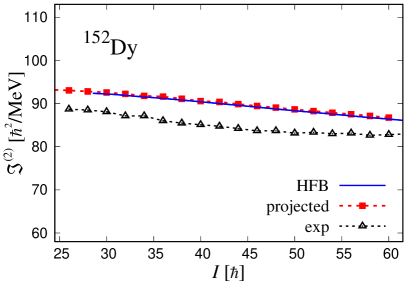
Figure 1: (Color online) Calculated ${\cal J}^{(2)}$ moment of inertia as a function of angular momentum for ¹⁵²Dy, where the result of projected multicranked configuration-mixing is drawn with symbols and that of cranked HFB calculated with Eq. (16) by the solid line. The experimental one is also included.

The results of multicranked configuration-mixing after projection and of the simple cranked HFB mean-field approximation shown in Fig. 1 are very similar. One may think that it is natural, but this is totally non-trivial and a consequence of the multicranked configuration-mixing as is shown in Fig. 2, where four ${\cal J}^{(2)}$ moments of inertia calculated from the spectra projected from a single mean-field state at each rotational frequency are depicted in addition to the final result of configuration-mixing. It can be seen that the values of these ${\cal J}^{(2)}$ moments of inertia are very similar and about $20-25$% smaller than the one obtained by the result of configuration-mixing, and, furthermore, they decrease more rapidly as functions of angular momentum. It seems that this is a general trend for the projected spectrum from a single HFB mean-field state STS15 ; STS16 , and indicates the importance of multicranked configuration-mixing for the proper description of the moment of inertia of the rotational band by the angular-momentum-projection method, especially for high-spin states.

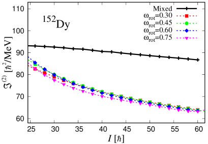
Figure 2: (Color online) ${\cal J}^{(2)}$ moments of inertia of projected spectra from a single cranked HFB state at each rotational frequency for ¹⁵²Dy. The result of configuration-mixing is also included.

It may be worthwhile mentioning that the ${\cal J}^{(2)}$ moment of inertia calculated by the projection from a single mean-field state shown in Fig. 2 corresponds to the so-called Yoccoz inertia, while the one calculated within the cranked HFB mean-field approximation, cf. Eq. (16), which agrees with the final result of projected configuration-mixing as shown in Fig. 1, corresponds to the Thouless-Valatin inertia, see Ref. RS80 . Thus, this result shows that the Yoccoz inertia is considerably smaller than the Thouless-Valatin inertia at least for the superdeformed rotational band at high-spin states; it is true not only for ¹⁵²Dy but also for ¹⁹⁴Hg as will be shown in Figs. 11 and 12 below.

In order to see why the result of configuration-mixing gives considerably larger value for ${\cal J}^{(2)}$ moment of inertia, the calculated spectra obtained by the projection from a single cranked HFB state at each rotational frequency as well as the result of the configuration-mixing are shown in Fig. 3, where the reference energy, $I(I+1)/190$ MeV, is subtracted. The ${\cal J}^{(2)}$ moment of inertia is the reciprocal of curvature of the spectral curve as a function of angular momentum, cf. Eq. (13). The result of configuration-mixing looks naturally like the envelope curve of a family of four spectral curves corresponding to those obtained with different frequencies, and consequently the curvature reduces from those of a family of curves. Note that each spectral curve obtained by projection from a single cranked HFB state with $\omega_{\rm rot}=\omega_{\rm rot}^{(n)}$ $(n=1,\cdots,4)$ comes in contact with this envelope-like curve at the spin value close to the cranked angular-momentum $I\approx\langle\Phi(\omega_{\rm rot}^{(n)})|J_{y}|\Phi(\omega_{\rm rot}^{(n)})\rangle$. The resultant spectrum of configuration-mixing is very similar to the one calculated by the cranked HFB as in the case of ${\cal J}^{(2)}$ moments of inertia shown in Fig. 1. In this way, the considerable increase of the ${\cal J}^{(2)}$ moment of inertia caused by the multicranked configuration-mixing can be naturally understood.

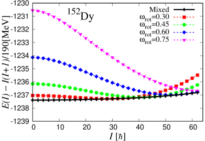
Figure 3: (Color online) Energy spectra of simple projections from a single cranked HFB state at each rotational frequency and that of the resultant configuration-mixing for ¹⁵²Dy. The reference energy, $I(I+1)/190$ MeV, is subtracted.

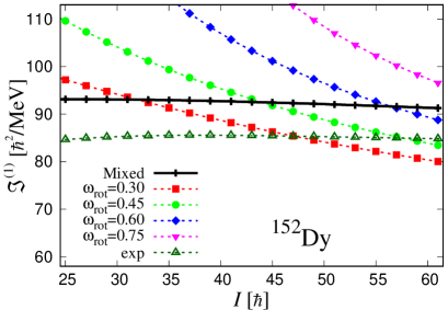
Figure 4: (Color online) ${\cal J}^{(1)}$ moments of inertia corresponding to the spectra in Fig. 3 for ¹⁵²Dy. The experimental one is also included.

In addition to the ${\cal J}^{(2)}$ moment of inertia in Fig. 1, the ${\cal J}^{(1)}$ moment of inertia is also useful for studying the properties of high-spin rotational bands. The calculated ${\cal J}^{(1)}$ moments of inertia corresponding to Fig. 3 are shown in Fig. 4, where the experimental one is also included. As seen from the figure, the value of the ${\cal J}^{(1)}$ moment of inertia is larger for the spectrum obtained by the projection from the mean-field state with higher rotational frequency. Those calculated by the projection from a single mean-field state are larger and decrease more rapidly than the corresponding ${\cal J}^{(2)}$ moments of inertia in Fig. 2. However, the value of the result of configuration-mixing is almost constant in agreement with the trend of the experimental data, although the calculated value of ${\cal J}^{(1)}$ is considerably (about 10%) overestimated. In this way, the projected spectrum from a single mean-field state does not give good description of the high-spin rotational band, and the multicranked configuration-mixing is crucial to obtain the correct magnitudes of both dynamic and kinematic moments of inertia for the superdeformed band in ¹⁵²Dy.

III.2.2 Projection from the mean-field determined by cranked VANP method

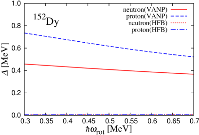
Figure 5: (Color online) Average pairing gaps as functions of the rotational frequency for ¹⁵²Dy, defined by Eq. (9) and calculated by the cranked HFB and VANP methods. Both neutron and proton gaps obtained by the HFB method vanish in the frequency range shown.

As it is discussed in Sec. II.2, the pairing phase-transition occurs suddenly at low spins with the static mean-field approximation like the HFB method. However, the effect of pairing fluctuations remains at rather high-spin states pairRMP ; YRS90 . An efficient method to take it into account is the VANP method, which determines the mean-field state according to Eq. (7). With the cranked VANP method, the obtained mean-field states have almost the same deformation as in the case of the cranked HFB method, $\beta_{2}=0.713$ and $0.698$ at $\hbar\omega_{\rm rot}=0.30$ and $0.75$ MeV, respectively. They are, however, in the superconducting phase with relatively weak pairing correlations, as is shown in Fig. 5, where the calculated average pairing gaps by Eq. (9) are depicted. The average pairing gaps for the neutron and proton obtained by the VANP method gradually decrease as functions of the rotational frequency and never vanish within the frequency range under consideration. These results are consistent with those in Ref. VER00 .

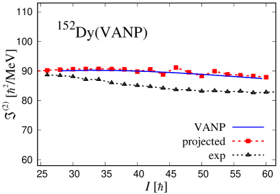
Figure 6: (Color online) Similar to Fig. 1 but the mean-field states obtained by the VANP method are utilized and the particle-number projection is also performed, cf. Eq. (5). Here the solid line is calculated by Eq. (18).

Utilizing four mean-field states obtained by this VANP method at the same cranking frequencies as in the case of the HFB method, $\hbar\omega_{\rm rot}=0.30,\,0.45,\,0.60,\,0.75$ MeV, the projected multicranked configuration-mixing has been carried out, where the particle-number is also projected out to the desired number for both the neutron and proton, see Eq. (5). A larger norm cut-off factor $10^{-9}$ is necessary to obtain a smooth rotational band. The resultant ${\cal J}^{(2)}$ moment of inertia is depicted in Fig. 6. Apparently, the result does not change very much from that with the cranked HFB method shown in Fig. 1, although it is almost constant as a function of angular momentum in contrast to the experimental data and the discrepancy slightly increases at higher frequency. The result of the simple cranked VANP approximation (the solid line) in Eq. (18) is again very similar to that of projected multicranked configuration-mixing as in the case of the HFB mean-field states being employed.

The calculated ${\cal J}^{(2)}$ moment of inertia by the projected configuration-mixing in Fig. 6 shows some small irregularities. This and other irregularities in the calculations seen in the present work are due to the fact that a small norm state in the Hill-Wheeler equation unfortunately comes in and/or goes out in the calculated spin range even though a relatively small value of norm cut-off parameter has been employed, in this case $10^{-9}$; usually its effect is small but it can be visible especially for the ${\cal J}^{(2)}$ moment of inertia that is the quantity of second derivative, see Eq. (13).

Figure 7: (Color online) Similar to Fig. 2 but the mean-field states obtained by the VANP method are utilized and the particle-number projection is also performed, cf. Eq. (5).

We show four ${\cal J}^{(2)}$ moments of inertia calculated from spectra projected from a single mean-field state at each rotational frequency in Fig. 7 with the result of configuration-mixing: They are rather similar to those obtained from the HFB mean-field states shown in Fig. 2, even though the average pairing gaps remain finite in the VANP mean-field states contrary to the vanishing pairing gaps in the HFB states. Thus, the effect of pairing fluctuations is not large for this nucleus. The calculated spectra of projection from a single cranked VANP state at each rotational frequency are displayed in Fig. 8 with the resultant spectrum of configuration-mixing. Note that the absolute energy of the projected configuration-mixing spectrum using the VANP states is about 3.7 MeV smaller at $I\approx 0$ because the particle-number projection is performed for both neutron and proton. The ${\cal J}^{(1)}$ moments of inertia corresponding to the spectra in Fig. 8 are also displayed in Fig. 9, where the experimental one is also included. The main features in Figs. 7$\sim$9 are not very different from the case utilizing the HFB mean-fields in Figs. 2$\sim$4.

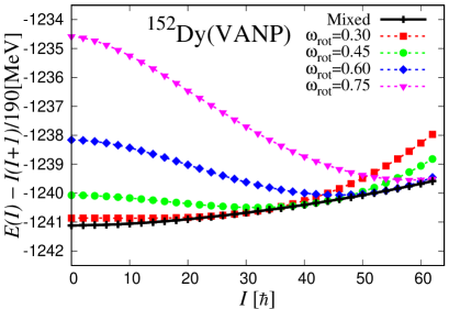
Figure 8: (Color online) Similar to Fig. 3 but the mean-field states obtained by the VANP method are utilized and the particle-number projection is also performed, cf. Eq. (5).

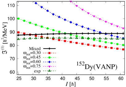
Figure 9: (Color online) Similar to Fig. 4 but the mean-field states obtained by the VANP method are utilized and the particle-number projection is also performed, cf. Eq. (5).

The difference between the results using the HFB and VANP mean-field states is that the values of cranked angular-momentum, see Eqs. (17) and (19), are systematically smaller in the results of the VANP states. In fact the resultant ${\cal J}^{(1)}$ moment of inertia by the configuration-mixing with the VANP method is reduced from that with the HFB method, and the agreement between the experimental data is improved, as it can be seen by comparing the ${\cal J}^{(1)}$ moments of inertia in Figs. 4 and 9. The importance of this “dealignment” effect and the reduction of ${\cal J}^{(1)}$ moment of inertia caused by the pairing fluctuations has been systematically investigated for normal deformed nuclei in Ref. pairRMP and for superdeformed nuclei in Refs. SVB90 ; NWJ89 . It can be easily understood by the fact that the correlation routhian induced by the pairing fluctuations, which is always negative, is increasing as a function of the rotational frequency and vanishes at infinite frequency. Then the correction due to the pairing fluctuations for ${\cal J}^{(1)}$ is always negative, cf. Eq. (12), in agreement with the analysis of Refs. SVB90 ; NWJ89 . For the ${\cal J}^{(2)}$ moment of inertia, the sign of correction term changes at the inflection point of the correlation routhian, because the ${\cal J}^{(2)}$ moment of inertia is defined by the second derivative, see e.g. Fig. 9 of Ref. SVB90 . Comparing the results of configuration-mixed spectra employing the HFB and VANP mean-field states, the inflection point of the correlation routhian exists at a rather high rotational frequency like $\hbar\omega_{\rm rot}\approx 0.5$ MeV, and the correction to ${\cal J}^{(2)}$ is negative before this frequency and positive after it, although the magnitude of correction to ${\cal J}^{(2)}$ is rather small; this result is slightly different from that in Ref. SVB90 .

III.3 Superdeformed band in ¹⁹⁴Hg

As an example of superdeformed bands in the $A\approx 190$ mass region, we take the yrast superdeformed band of the ¹⁹⁴Hg nucleus, which has been observed in an early stage of superdeformation-hunting in this region Hg194sp , and the spin-assignment has been given afterward Hg194SD . We have performed the multicranked configuration-mixing calculation using four cranked mean-field states at the rotational frequencies, $\hbar\omega_{\rm rot}=0.10,\,0.23,\,0.36,\,0.49$ MeV, which cover the spin-range of the measured rotational band in ¹⁹⁴Hg.

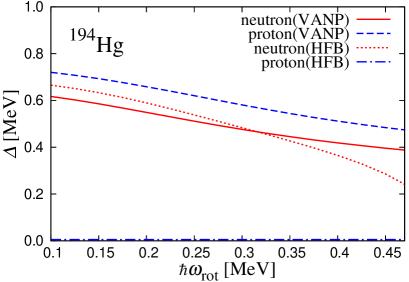
Figure 10: (Color online) Average pairing gaps as functions of the rotational frequency for ¹⁹⁴Hg, defined by Eq. (9) and calculated by the cranked HFB and VANP methods. Proton gap obtained by the HFB method vanishes in the frequency range shown.

Generally speaking, the pairing correlations are weak due to the relatively large shell gaps resulting from the (approximate) rational axis ratio 2:1 for the long- to short-axis in the superdeformed states BM75 . The values of deformation for the superdeformed states in the $A\approx 190$ region are smaller than those in the $A\approx 150$ region, see e.g. Ref. Chas89 , and the shell gaps in the $A\approx 190$ region are suggested to be slightly smaller. Because of this, the pairing correlations are expected to be relatively stronger for nuclei in the $A\approx 190$ region than those in the $A\approx 150$ region, see e.g. Ref. BFH90 . The calculated average pairing gaps for ¹⁹⁴Hg are shown in Fig. 10 as functions of the rotational frequency. The proton gap obtained by the HFB method vanishes already at $\hbar\omega_{\rm rot}=0.10$ MeV, while the neutron gap remains at higher frequency. As in the case of ¹⁵²Dy shown in Fig. 5, both pairing gaps for both neutron and proton obtained by the VANP method are finite and gradually decrease as functions of the rotational frequency. These results are very similar to those in Ref. VER00 . The neutron gap with the HFB method decreases more rapidly than that with the VANP method. The values of the average gaps in ¹⁹⁴Hg and ¹⁵²Dy calculated with the VANP method are similar for protons, and the value in ¹⁹⁴Hg is larger for neutrons. Considering the general mass dependence of the pairing gap, $\propto 1/\sqrt{A}$, the pairing correlations deduced from the calculated pairing gaps are stronger in ¹⁹⁴Hg than in ¹⁵²Dy especially for neutrons.

III.3.1 Projection from the mean-field determined by cranked HFB method

Our Gogny HFB calculation gives a superdeformed minimum in ¹⁹⁴Hg with $\beta_{2}=0.548$ and $0.529$ at $\hbar\omega_{\rm rot}=0.10$ and $0.49$ MeV, respectively. Again, the axial-symmetry is kept very well up to high rotational frequency. The calculated ${\cal J}^{(2)}$ moment of inertia by the configuration-mixing using the four cranked HFB mean-fields states is shown in Fig. 11, where the result of simple HFB approximation, cf. Eq. (16), and the experimental one are also included. The small norm cut-off factor $10^{-12}$ works in this calculation. In contrast to the case of ¹⁵²Dy, where the ${\cal J}^{(2)}$ moment of inertia is almost constant or even gradually decreases, the calculated ${\cal J}^{(2)}$ moment of inertia for ¹⁹⁴Hg increases as a function of angular momentum, which clearly shows the importance of the pairing correlation. However, the amount of increase is considerably smaller in comparison with the experimental data. It should be mentioned that the result of the HFB mean-field approximation (the solid line) is very similar to that calculated by the multicranked configuration-mixing just like the case of ¹⁵²Dy.

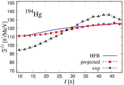
Figure 11: (Color online) Calculated ${\cal J}^{(2)}$ moment of inertia as a function of angular momentum for ¹⁹⁴Hg, where the result of projected multicranked configuration-mixing is drawn with symbols and that of cranked HFB mean-field with Eq. (16) by the solid line. The experimental one is also included.

In order to see the effect of configuration-mixing, four ${\cal J}^{(2)}$ moments of inertia calculated from the spectra obtained by the projection from a single cranked HFB state at each rotational frequency are displayed in Fig. 12, where the final result of configuration-mixing is also included. As in the case of ¹⁵²Dy in Fig. 2, they take similar values except for at lower spin values $I\mathrel{\hbox{\raise 0.86108pt\hbox{$<$}\kern-7.5pt\raise-3.87495pt\hbox{$\sim$}}}20$, and they gradually decrease as functions of angular momentum. The average values of four ${\cal J}^{(2)}$ moments of inertia at high-spin states calculated by the projection from a single cranked mean-fields state are considerably smaller than the value obtained by the final configuration-mixing. Moreover, the dependence on the angular momentum completely changes as a result of configuration-mixing for ¹⁹⁴Hg, which leads to the increase in accordance with the experimental data.

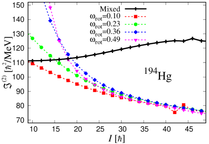
Figure 12: (Color online) ${\cal J}^{(2)}$ moments of inertia of projected spectra from a single cranked HFB state at each rotational frequency for ¹⁹⁴Hg. The result of configuration-mixing is also included.

Furthermore, the calculated spectra from a single cranked HFB state at each rotational frequency are depicted in Fig. 13 with the result of final configuration-mixing; the reference energy, $I(I+1)/240$ MeV, is subtracted for ¹⁹⁴Hg. The resultant spectral curve after the configuration-mixing follows the envelope curve of the four spectral curves obtained by the projection from a single mean-field state with $\omega_{\rm rot}=\omega_{\rm rot}^{(n)}$ $(n=1,\cdots,4)$, and comes in contact with each spectral curve at $I\approx\langle\Phi(\omega_{\rm rot}^{(n)})|J_{y}|\Phi(\omega_{\rm rot}^{(n)})\rangle$. Consequently, its curvature is becoming smaller, or the ${\cal J}^{(2)}$ moment of inertia is becoming larger, as a result of configuration-mixing.

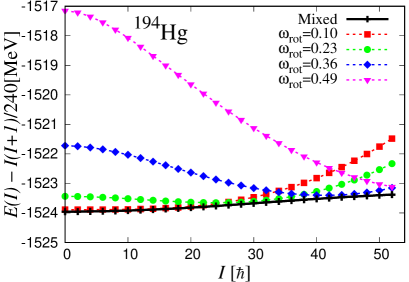
Figure 13: (Color online) Energy spectra of simple projections from a single cranked HFB state at each rotational frequency and that of the resultant configuration-mixing for ¹⁹⁴Hg. The reference energy, $I(I+1)/240$ MeV, is subtracted.

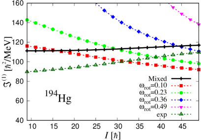
Figure 14: (Color online) ${\cal J}^{(1)}$ moments of inertia corresponding to the spectra in Fig. 13 for ¹⁹⁴Hg. The experimental one is also included.

In Fig. 14 the ${\cal J}^{(1)}$ moments of inertia calculated by the projection from a single mean-field state are compared with those by the final configuration-mixing and by the experimental data. As in the case of ¹⁵²Dy, the four calculated ${\cal J}^{(1)}$ moments of inertia obtained by the projection from a single mean-field state quickly decrease as spin increases. The spin-dependence of the result of final configuration-mixing changes, i.e., the resultant ${\cal J}^{(1)}$ moment of inertia increases as spin, which well corresponds well to the trend of the experimental data, although the absolute value is considerably overestimated compared to the experimental data. Thus, the ${\cal J}^{(1)}$ and ${\cal J}^{(2)}$ moments of inertia calculated by the projection from a single mean-field state with each rotational frequency are very different from the experimentally measured moments of inertia for both the absolute value and the spin-dependence. Again, the effect of multicranked configuration-mixing is essential to understand the observed behavior of the rotational spectrum and two moments of inertia.

III.3.2 Projection from the mean-field determined by cranked VANP method

In order to see the effect of dynamic pairing correlations, we have performed the angular-momentum-projection calculations employing the mean-field states obtained by the VANP method for ¹⁹⁴Hg; the particle-number projection is also performed in this case, cf. Eq. (5). The calculated values of deformation parameter for superdeformed minimum are $\beta_{2}=0.545$ and $0.530$ at $\hbar\omega_{\rm rot}=0.10$ and $0.49$ MeV, respectively, which are essentially the same as those calculated with the HFB method. With the four mean-field states obtained by the cranked VANP method at the same cranking frequencies as those by the cranked HFB method, $\hbar\omega_{\rm rot}=0.10,\,0.23,\,0.36,\,0.49$ MeV, the multicranked configuration-mixing calculation has been carried out with the result shown in Fig. 15. A larger norm cut-off factor $10^{-10}$ is necessary to obtain smooth rotational band. As it is clearly seen, the result employing the VANP mean-field states is slightly changed from the one employing the HFB mean-field states shown in Fig. 11: The calculated ${\cal J}^{(2)}$ moment of inertia is reduced at lower spin and is increased at higher spin in comparison with the one obtained with the HFB mean-field states, and the agreement with the experimental data is better. Again, the results of projected configuration-mixing and of the cranked VANP approximation (the solid line) calculated by Eq. (18) are very similar.

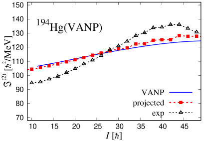
Figure 15: (Color online) Similar to Fig. 11 but the mean-field states obtained by the VANP method are utilized and the particle-number projection is also performed, cf. Eq. (5). Here the solid line is calculated by Eq. (18).

Figure 16 shows four ${\cal J}^{(2)}$ moments of inertia calculated from the projected spectra obtained by a single cranked VANP mean-field state at each rotational frequency in addition to the result of final configuration-mixing. The ${\cal J}^{(2)}$ moments of inertia calculated by the projection from a single mean-field state with the VANP method are not so different from those with the HFB method shown in Fig. 12, although the result of configuration-mixing more rapidly increases as a function of angular momentum; this also suggests the importance of multicranked configuration-mixing.

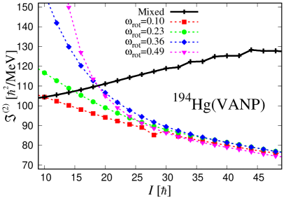
Figure 16: (Color online) Similar to Fig. 12 but the mean-field states obtained by the VANP method are utilized and the particle-number projection is also performed, cf. Eq. (5).

To see the effect of configuration-mixing, we show in Fig. 17 the four calculated spectra from a single VANP mean-field state at each rotational frequency in addition to the result of configuration-mixing. The absolute energy of the projected configuration-mixing spectrum from the VANP states is about 3.4 MeV smaller at $I\approx 0$ due to the particle-number projection on top of the angular-momentum projection. Again, the result of configuration-mixing follows the envelope curve of a family of four spectral curves obtained by the projection from a single cranked VANP mean-field states. Compared to the results with the HFB mean-field states, the spin and the energy values at their contacting points are smaller and larger, respectively, for the VANP method, and consequently the curvature of the parabolic spectrum of the final configuration-mixing is larger at lower spin, while it is smaller at higher spin. This leads to reduction of the ${\cal J}^{(2)}$ moment of inertia at lower spin and increase at higher spin as a result of multicranked configuration-mixing using the VANP mean-field states.

Figure 17: (Color online) Similar to Fig. 13 but the mean-field states obtained by the VANP method are utilized and the particle-number projection is also performed, cf. Eq. (5).

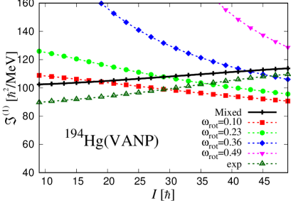
Figure 18: (Color online) Similar to Fig. 14 but the mean-field states obtained by the VANP method are utilized and the particle-number projection is also performed, cf. Eq. (5).

In the same way, the ${\cal J}^{(1)}$ moments of inertia calculated from the spectra obtained by a single VANP mean-field state at each cranking frequency and the result of configuration-mixing are displayed in Fig. 18 corresponding to the spectra in Fig. 17. The experimental ${\cal J}^{(1)}$ moment of inertia is also included. It is clearly seen that the resultant ${\cal J}^{(1)}$ moment of inertia by configuration-mixing employing the VANP mean-field states is reduced compared with the result using the HFB mean-field states shown in Fig. 14. Consequently, the agreement with the experimental data is better in the result with the VANP mean-field states. This reduction of the ${\cal J}^{(1)}$ moment of inertia is in agreement with the general analysis of the pairing fluctuations at high-spin states in Refs. pairRMP ; YRS90 , where the systematic dealignment effect has been recognized. Thus the effect of dynamic pairing correlations is not very large also for ¹⁹⁴Hg; these results are slightly different from those in Ref. VER00 .

III.3.3 No number projection with cranked VANP method

The numerical cost to perform both the particle-number and angular-momentum projection at the same time is very large. On the other hand, the effect of the number projection is usually not very large, see e.g. Ref. HS95 . We have also confirmed it in the calculation of the spectrum for a tetrahedrally deformed nucleus TSD13 . Therefore, we try the multicranked configuration-mixing calculation with no particle-number projection by employing the VANP mean-field states. The result for the ${\cal J}^{(2)}$ moment of inertia is depicted in Fig. 19, where the four ${\cal J}^{(2)}$ moments of inertia calculated by the projection from a single VANP mean-field state at each rotational frequency are also included. The norm cut-off factor $10^{-12}$ can be used in this calculation.

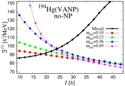
Figure 19: (Color online) Similar to Fig. 16 but no particle-number projection is performed.

Compared with the corresponding result shown in Fig. 16, the resultant ${\cal J}^{(2)}$ moment of inertia of configuration-mixing is very different. The increase as a function of the rotational frequency is much larger; even larger than that of the experimental data. In contrast, those calculated with a single mean-field state are not very different from the case with particle-number projection. In order to understand the reason for it, the four spectra calculated from the projection from a single mean-field state are displayed in Fig. 20 in addition to the resultant spectra of configuration-mixing. Note that the absolute energies of the projected spectra are even larger than those using the HFB states shown in Fig. 13, because the particle-number projection is not performed with the VANP mean-field states. It can be seen that the spectral curves obtained by the projection from a single mean-field state are not very different from those calculated with number projection shown in Fig. 17, which is consistent with the observation that the effect of number projection is not very important in Ref. TSD13 , where the projection was performed from a single mean-filed state. However, the resultant spectrum of configuration-mixing is dramatically changed if no particle-number projection is performed.

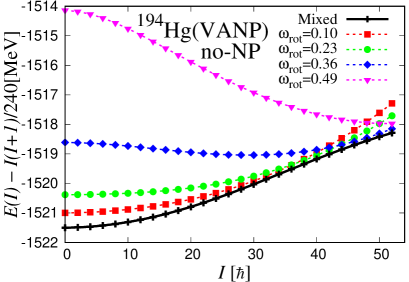
Figure 20: (Color online) Similar to Fig. 17 but no particle-number projection is performed.

It is worthwhile mentioning that the energy gain caused by the configuration-mixing seen in Fig. 20 is considerably larger than those in Figs. 13 and 17, especially at low spin, $I\mathrel{\hbox{\raise 0.86108pt\hbox{$<$}\kern-7.5pt\raise-3.87495pt\hbox{$\sim$}}}20$. This indicates that the coupling matrix elements in the Hill-Wheeler equation in Eq. (3) are overestimated when the number projection is not carried out for the VANP mean-field states. If the HFB mean-field state with cranking frequency $\omega^{(n^{\prime})}_{\rm rot}$ is represented by the quasiparticle states of the other HFB state with $\omega^{(n)}_{\rm rot}$, their coupling matrix elements consists of the terms between the zero quasiparticle state and the two, four, six, $\cdots$ quasiparticle states. However, those between the zero and two quasiparticle states, which are considered to contribute most owing to the small energy denominators, vanish because of the selfconsistency condition of the HFB, i.e. vanishing “dangerous terms”, see e.g. Ref. RS80 . A similar result applies true also for the VANP mean-field states but with respect to “number projected” quasiparticle states. Therefore, the coupling terms of configuration-mixing are supposed to be small if the mean-field states are determined selfconsistently as in the cases shown in Fig. 13 for the HFB method and in Fig. 17 for the VANP method. This is not the case, however, if the number projection is neglected for the configuration-mixing using the VANP mean-field states in Fig. 20. In this way, although the effect of number projection is not very important for the projection from a single VANP mean-field state, its effect can be rather large for the configuration-mixing like in the present case. Thus, we should be careful about employing any kind of approximations which break the selfconsistently of mean-field states if the multicranked configuration-mixing is performed. Although the effect of breaking the selfconsistency is found to be not so large for the case of another nucleus ¹⁵²Dy (not shown) as in the case of ¹⁹⁴Hg, the same caution should be applied. In fact, the results of final configuration-mixing do not agree with the cranked VANP approximation in Eq. (18) in both ¹⁵²Dy and ¹⁹⁴Hg cases, if the number projection is not performed for the VANP states.

IV Conclusion

The nuclear mean-field theory is one of the most successful theories to describe nuclear properties from the microscopic view point. The key concept is the spontaneous symmetry breaking, where complicated correlations between the constituent nucleons can be incorporated through the nuclear mean-field. To obtain the quantum mechanical eigenstates, however, one has to restore the symmetry broken in the mean-field: The nuclear mean-field is the intrinsic state, from which a series of symmetry-preserving eigenstates is generated by the quantum-number projection method. The collective rotation is a good example; a sequence of eigenstates composing the rotational band is obtained by the angular-momentum projection from a single deformed mean-field state. Although it is conceptually correct and appealing, the result of projection from a single mean-field state is not enough for precise description of the rotational band especially at high-spin states, which is clearly indicated in the present work. It is necessary to make multicranked configuration-mixing, i.e., several mean-field states with different cranking frequencies should be properly superposed after angular-momentum projection.

Thus, we show how the approach of projected multicranked configuration-mixing works for the good description of high-spin rotational bands. This approach, cf. Eq. (1) or Eq. (2), has been originally proposed by Peierls and Thouless PT62 and developed recently in our previous works STS15 ; STS16 . In the present work, it is applied to the investigation of superdeformed bands in the ¹⁵²Dy and ¹⁹⁴Hg nuclei, where long rotational sequences are observed and the spin-assignments have been provided. These two representative nuclei are chosen to investigate the effect of pairing fluctuations on the ${\cal J}^{(2)}$ moment of inertia of the superdeformed band, for which large difference has been known between the $A\approx 150$ and $A\approx 190$ mass regions. The two methods to incorporate the pairing correlations, i.e., the HFB and the VANP methods, are employed to determine the mean-field states, with which the angular-momentum projection (and the particle-number projection at the same time for the VANP method) and subsequent configuration-mixing is performed. The Gogny D1S force is used as the effective interaction. The different behavior of the ${\cal J}^{(2)}$ moment of inertia in ¹⁵²Dy and ¹⁹⁴Hg is attributed to the effect of pairing correlations, which is stronger in ¹⁹⁴Hg than in ¹⁵²Dy. This is consistent with other previous works, see e.g. Ref. VER00 , in which the angular-momentum projection is not considered though.

It is demonstrated that the configuration-mixing of several mean-field states with different cranking frequencies are essential to understand the ${\cal J}^{(1)}$ and ${\cal J}^{(2)}$ moments of inertia of superdeformed nuclei by the angular-momentum-projection calculation. The projection calculation from a single mean-field state obtained by either the HFB or VANP method does not give any reasonable results; the calculated ${\cal J}^{(2)}$ moments of inertia are too small and decrease gradually as functions of angular momentum. With configuration-mixing after projection, fair agreement with experimental data is achieved for both the ${\cal J}^{(1)}$ and ${\cal J}^{(2)}$ moments of inertia, although the agreement is not perfect in the present investigation. A selfconsistent treatment is emphasized for the configuration-mixing; namely, both the particle-number and angular-momentum projection are necessary if the VANP mean-field states are employed. With proper selfconsistency, however, the results of the multicranked configuration-mixing for ${\cal J}^{(2)}$ moments of inertia are found to be very similar to those calculated with the semiclassical cranked HFB or VANP approximation without angular-momentum projection. This means that the mean-field approximation (or its extension like VANP) gives a fairly good approximation for the description of superdeformed high-spin rotational bands.

References

- (1) A. Bohr and B. R. Mottelson, Nuclear Structure, Vol. II Benjamin, New York (1975).
- (2) P. Ring and P. Schuck, The Nuclear Many-Body Problem, Springer, New York (1980).
- (3) M. J. A. de Voigt, J. Dudek, and Z. Szymanski, Rev. Mod. Phys. 55, 949 (1983).
- (4) J. D. Garrett, G. B. Hagemann, and B. Herskind, Ann. Rev. Nucl. Part. Sci. 36, 419 (1986).
- (5) S. Frauendorf, Rev. Mod. Phys. 73, 463 (2001).
- (6) D. Ward and P. Fallon, Advances in Nuclear Physics, vol. 26, Chap. 3, 167 (2001).
- (7) W. Satuła and R. A. Wyss, Rep. Prog. Phys. 68, 131 (2005).
- (8) S. Frauendorf, Phys. Scr. 93, 043003 (2018).
- (9) M. Shimada, S. Tagami, and Y. R. Shimizu, Prog. Theor. Exp. Phys. 2015, 063D02 (2015).
- (10) M. Shimada, S. Tagami, and Y. R. Shimizu, Phys. Rev. C 93, 044317 (2016).
- (11) K. Hara and Y. Sun, Int. J. Mod. Phys. E 04, 637 (1995).
- (12) Y. Sun, Phys. Scr. 91, 043005 (2016).
- (13) J. A. Sheikh, G. H. Bhat, W. A. Dar, S. Jehangir, and P. A. Ganai, Phys. Scr. 91, 063015 (2016).
- (14) R. E. Peierls and D. J. Thouless, Nucl. Phys. 38, 154 (1962).
- (15) S. Tagami and Y. R. Shimizu, Phys. Rev. C 93, 024323 (2016).
- (16) M. Borrajo, T. R. Rodríguez, J. L. Egido, Phys. Lett. B 746, 341 (2015).
- (17) P. J. Twin et al., Phys. Rev. Lett. 57, 811 (1986).
- (18) P. J. Nolan and P. J. Twin, Annu. Rev. Nucl. Part. Sci. 38, 533 (1988).
- (19) R. V. F. Janssens and T. L. Khoo, Annu. Rev. Nucl. Part. Sci. 41, 321 (1991).
- (20) C. Baktash, B. Haas, and W. Nazarewicz, Annu. Rev. Nucl. Part. Sci. 45, 485 (1995).
- (21) A. Bohr and B. R. Mottelson, Phys. Scr. 24, 71 (1981).
- (22) S. Tagami and Y. R. Shimizu, Prog. Theor. Phys. 127, 79 (2012).
- (23) J. Dechargé and D. Gogny, Phys. Rev. C 21, 1568 (1980).
- (24) J. F. Berger, M. Girod, and D. Gogny, Comput. Phys. Commun. 63, 365 (1991).
- (25) J. L. Egido, Phys. Scr. 91, 073003 (2016).
- (26) A. Kerman and N. Onishi, Nucl. Phys. A 361, 179 (1981).
- (27) S. Frauendorf, Nucl. Phy. 557, 259c (1993).
- (28) S. Frauendorf, Nucl. Phy. 677, 115 (2000).
- (29) Y. R. Shimizu, J. D. Garrett, R. A. Broglia, M. Gallardo and E. Vigezzi, Rev. Mod. Phys. 61, 131 (1989).
- (30) Y. R. Shimizu, P. Donati and R. A. Broglia, Phys. Rev. Lett. 85, 2260 (2000).
- (31) D. Almehed, F. Dönau, S. Frauendorf, and R. G. Nazmitdinov, Phys. Scr. T88, 62 (2000).
- (32) Y. R. Shimizu, E. Vigezzi, and R. A. Broglia, Nucl. Phys. A 509, 80 (1990).
- (33) C. Federschmidt and P. Ring, Nucl. Phys. A 435, 110 (1985).
- (34) Y. R. Shimizu and R. A. Broglia, Nucl. Phys. A515, 38 (1990).
- (35) Y. R. Shimizu, Nucl. Phys. A 520, 477c (1990).
- (36) W. Nazarewicz, R. Wyss, and A. Johnson, Nucl. Phys. A 503, 285 (1989).
- (37) J. Terasaki, P. -H. Heenen, P. Bonche, J. Dobaczewski, and H. Flocard, Nucl. Phys. A 593, 1 (1995).
- (38) P. Bonche, H. Flocard, and P. -H. Heenen, Nucl. Phys. A 598, 169 (1996).
- (39) M. Girod, J. P. Delaroche, and J. F. Berger, Phys. Lett. B 325, 1 (1994).
- (40) A. Valor, J. L. Egido, and L. M. Robledo, Nucl. Phys. A 665, 46 (2000).
- (41) A. V. Afanasjev, J. König, and P. Ring, Nucl. Phys. A 608, 107 (1996).
- (42) J. A. Sheikh and P. Ring, Nucl. Phys. A 665, 71 (2000).
- (43) T. Inakura, S. Mizutori, M. Yamagami, and K. Matsuyanagi, Nucl. Phys. A 710, 261 (2002).
- (44) M. Bender, K. Rutz, P.-G. Reihard, and J. A. Maruhn, Eur. Phys. J. A 8, 59 (2000).
- (45) B. Singth, R. Zywina, and R. B. Firestone, Nuclear Data Sheets, 97, 241 (2002).
- (46) T. R. Werner and J. Dudek, At. Data and Nuclear Data Tables, 50, 179 (1992).
- (47) T. R. Werner and J. Dudek, At. Data and Nuclear Data Tables, 59, 1 (1995).
- (48) J. Dudek, W. Nazarewicz, and P. Olanders, Nucl. Phys. A 420, 285 (1984).
- (49) T. Lauritsen et al., Phys. Rev. Lett. 88, 042501 (2002).
- (50) M. A. Riley et al., Nucl. Phys. A 512, 178 (1990).
- (51) T. L. Khoo et al., Phys. Rev. Lett. 76, 1583 (1996).
- (52) R. R. Chasmann, Phys. Lett. B 219, 227 (1989).
- (53) P. Bonche, J. Dobaczewski, H. Flocard, P.-H. Heenen, and J. Meyer, Nucl. Phys. A510 (1990), 466.
- (54) S. Tagami, Y. R. Shimizu, and J. Dudek, Phys. Rev. C 87, 054306 (2013).